Agricultural Land Price Convergence: Evidence from Polish Provinces

Abstract

This research deals with the problem of agricultural land market efficiency using the spatial market integration concept as well as the present value (PV) model. Empirically, it aims to test the convergence of agricultural land prices across Polish provinces. In order to check the law of one price (LOP), good-quality, medium-quality and bad-quality land sales markets are examined separately. Furthermore, this study is complemented by an analysis of the drivers behind agricultural land price convergence. The main method of testing price convergence is the log t regression. The latter was performed in two configurations, i.e., based on trend components of time series extracted using the Hodrick–Prescott filter and the Hamilton filter. Additionally, traditional β- and σ-convergence tests were applied. The obtained results indicated that agricultural land prices tend to converge in relative terms, which means that the provinces share a common long-run growth path. This finding and estimates of traditional convergence tests prove the increasing integration in the agricultural land market in Poland. There is no evidence, however, to support the conclusion that the absolute version of the long-run LOP holds. Moreover, using dynamic fixed effects models, it was identified that for good-, medium- and bad-quality land prices almost the same drivers of convergence apply. The only differences concern the strength of the influence of independent variables on prices of farmland of various types. Additionally, bad-quality land prices are the only ones which are affected by livestock density. Furthermore, estimates of the present value model finally confirmed that the agricultural land sales market in Poland cannot be considered as efficient.

1. Introduction

Agricultural land is of considerable importance, since it is both one of the three production factors [1] and also a means of production [2]. Compared to other production factors, land has a very specific character. Above all, land is key in meeting the subsistence needs of people around the world [3]. In addition, land is immobile, indestructible and, ultimately, its resources are limited [4]. In the face of growing urbanisation, agricultural land is decreasing from year to year [2]. This has a very strong impact on legislation on the marketing of agricultural land. In particular, many countries, for fear of raising agricultural land prices and non-agricultural land use, have introduced regulations restricting trade on the agricultural land market. For example, as noted by Yang et al. [5], in 2014, restrictions concerning agricultural land sales were introduced in Belgium and Slovakia. Similarly, in Poland, in 2016, it was decided to constrain heavily the possibility of purchasing agricultural land on the private market, while the sale of state agricultural land resources was suspended for a period of five years. This new agricultural policy was aimed at limiting the speculative buyout of agricultural land by investors, especially foreign ones. However, the imposed regulations are so far-reaching that, according to the European Commission, they restrict the free movement of capital, freedom of establishment and the freedom to choose one’s place of residence, which is contrary to EU law. Moreover, in the context of these new rules mentioned above, the term “speculation” is not a proven fact, but rather a political value judgement that is made by the government. However, from a scientific perspective, investments into land from outside agriculture can bring some benefits, such as additional money for farmers to retire or to improve farm-management. Furthermore, as Grau et al. [6] indicates, the results of academic research question the enforcement of such strict regulations.

The above premises reveal the extent of the complexity of the agricultural land market, which very often is subjected to state intervention aimed at achieving better results and eliminating market failure. Market failures in the agricultural land market are identified through the assessment of its efficiency [7]. If the land market operates efficiently, agricultural development takes place. When the land market is not functioning correctly, no optimal allocation of resources takes place, which leads to a decrease in overall efficiency and welfare [8].

The scientific literature distinguishes between two perspectives in land market efficiency research. The first concerns the analysis of rents [9], and the second uses the concept of spatial market integration [7]. The theoretical basis of the former is the present value (PV) model according to which the price of an asset is equal to all future expected earnings from the asset [10]. In the context of farmland, the PV model represents a current price of land as the stream of future rents [11], which can be obtained from the use of land for productive activities [8]. When the market price of the land deviates from its fundamental value determined by returns, the agricultural land market cannot be considered as efficient [12]. The lack of a stable long-term relationship between land prices and rents may result from speculative activities as well as other factors, such as taxation, transactions costs, liquidity constraints or institutional framework [8]. However, the use of the PV model to assess the efficiency of land market may be problematic mainly due to the difficulty of selecting the discount rate, which may vary significantly over time. Moreover, in many countries, data on agricultural land rental prices are not available.

In the case of spatially efficient markets, on the other hand, a shock causing a price differential in these markets will be temporary, and over time prices tend to equalize [13]. Therefore, from an empirical perspective, one can speak of a process of price convergence [14,15]. As Carmona and Rosés point out [8], in the absence of land market integration, real estate prices deviate from their fundamentals. Moreover, in this type of situation, riskless profit opportunities for spatial traders are created [16]. It should be noted that the spatial integration concept is based on the law of one price (the LOP) [14], which holds when markets are integrated. The LOP occurs in strong (short-run) and weak (long-run) versions. The first assumes that prices of homogeneous goods across spatially separated markets are the same. The second allows for price differentials between markets but also postulates a long-run relationship between prices [17]. The lack of automatic elimination of different price levels between locations is due, among other things, to transaction costs that inhibit arbitrage. It should be noted that under the long-run LOP, absolute or relative-LOP can be defined [18]. The latter implies a constant difference between prices across markets. In the case of absolute-LOP, the above-mentioned difference will disappear completely in the long run.

With regard to the concept of spatial market integration in agricultural land markets, it is very likely that the strong version of the LOP does not hold. Some indications, however, can be given that the long-run LOP may be present in this case. As Twardowska notes [19], the above situation may be a consequence of the existing integration in agricultural commodity markets, which has been proven in many studies to date [20,21,22]. Moreover, spatial equilibrium in the agricultural land market may be the result of capital and/or farm managers’ mobility [7]. Conversely, the agricultural land market is part of the real estate market, which is characterised by locality and heterogeneity [23,24,25], both of which may hinder integration processes.

Although interest in the subject of agriculture is high across the scientific literature, analyses of the convergence of agricultural land prices are rare. Among relevant studies conducted so far, the research of Yang et al. [5,7] for agricultural land in Germany should be noted. Using panel data unit root and stationarity tests, as well as a price diffusion model, the authors concluded that, in the German state of Lower Saxony, the law of one price holds only locally. A similar study using the land price diffusion model with an error correction specification was carried out by Grau et al. [6] who concluded that local agricultural land markets in Germany are spatially integrated; however, land prices do not tend to move towards the same level, but rather show relative convergence. In turn, analysing the Spanish land market, Carmona and Rosés [8] found the existence of price convergence across all studied provinces. A survey of convergence of agricultural land prices was also conducted by Twardowska [19]. The author inferred that there is significant decrease in the differentiation of farmland prices among the countries of the European Union between 2006 and 2016, which indicates the existence of sigma convergence. On the basis of the above, it must be concluded that the problem concerning agricultural land market efficiency is under-researched. In particular, there are no studies on the convergence of farmland prices in Poland. Therefore, the aim of this study is to analyse the processes of convergence of agricultural land prices across all Polish provinces, as well as to identify the driving forces of convergence (or divergence). In order to examine convergence, the log t regression test will be used, which assesses whether prices converge to a single long-term equilibrium or whether multiple equilibria (i.e., convergence clubs) exist. Furthermore, on the basis of this method, it can be concluded whether absolute or relative convergence is taking place. To the best of our knowledge, this is the first study to test the convergence of agricultural land prices using the above-mentioned method. Additionally, traditional convergence tests, i.e., σ- and β-convergence models, will be performed.

It should be noted that bubbles and fads in the agricultural land market can affect the whole nation. Therefore, the convergence of agricultural land prices may be caused by non-fundamental factors. Taking all the above into account, it should be concluded that the efficient agricultural land market is characterised by the existence of a price convergence process in which the LOP holds. Additionally, this process must be driven by market fundamentals, i.e., land prices mimic changes in rents (or their proxy) with a long-term elasticity equal to one [8]. On this basis, a second objective of this study is to identify the driving forces of the convergence of agricultural land prices in Poland. The latter goal will be carried out in two stages. The first will identify determinants which affect supply and demand in the agricultural land sales market and, in consequence, may significantly shape the prices of agricultural plots. In the second, the PV model will be used to explain price volatility. The former and the latter stages will answer the question to what extent agricultural land prices are driven by market fundamentals (rents) and to what extent by determinants of a different nature. It should be stressed, however, that the above study will only be a starting point for further empirical analysis due to the large data availability constraints.

This research contributes to the existing scant literature in several ways. Firstly, this analysis examines for the first time the problem of efficiency of the agricultural land market in Poland by investigating the convergence of farmland prices and their behaviour in relation to market fundamentals (rents). Secondly, the recently developed methodology (the log t regression) outlined by Phillips and Sul [26,27] is used to test the convergence of agricultural land prices and to identify potential convergence clubs. It should be stressed that the log t regression has so far only been used to analyse the convergence of housing prices, but also in this case the scientific literature is scarce. Thirdly, in order to take into account the heterogeneity of agricultural land, the efficiency study is carried out separately for good, medium and bad-quality land.

The paper is organised as follows. Section 2 explains the methodology of testing land price convergence and its driving forces, as well as data used in the empirical survey. Section 3 contains a description of the research results and a discussion. The final section formulates the main conclusions of the study, and indicates the limitations and directions for future research.

2. Methodology and Data

2.1. Methodology of Testing Agricultural Land Price Convergence

In order to study agricultural land price convergence across Polish provinces, three convergence tests will be used. The first consists in verifying whether provinces with low initial land prices can achieve high land price growth rates. In this case, it can be concluded that an unconditional convergence across provinces is present. The above can be empirically checked by the so-called β-convergence model, which takes the following form [28]:

$$\frac{\ln \left(\frac{p_{iT}}{p_{i0}}\right)}{T}=\gamma +\beta \ln p_{i0}+{\epsilon }_i$$

(1)

where $p_{iT}$ denotes average agricultural land price in province $i \left(i=1,\dots ,N\right)$ at time $T$ ($t=1,\dots ,T$), $p_{i0}$ is the initial average agricultural land price in province $i$, ${\epsilon }_i$ is the error term, $\gamma$ denotes the constant of the model, and $\beta$ is the slope coefficient whose significance and negative value indicates the existence of convergence. It should be noted that modifying Equation (1) by means of adding a set of control variables would cause a conditional convergence to be checked. It should be stressed that the β-convergence model does not verify the process of changing price level differentials between provinces, which forces the use of other convergence examination methods when analysing the law of one price.

The second approach of testing convergence is based on the analysis of the cross-sectional standard deviation of land prices. In this case, the σ-convergence concept is used, which assumes the presence of convergence if the above-mentioned standard deviation decreases over time. The latter indicates that there is a process of equalisation of price levels across localisations. Taking into account both β-convergence and σ-convergence, it should be stressed that the former is a necessary but not sufficient condition for the latter [29].

It should be noted, however, that both β-convergence and σ-convergence tests are not adequate for studying agricultural land price convergence. This results from the fact that these methods provide little information, while the slope parameter from Equation (1) is biased due to the problems of omitted variables and endogeneity [30].

Therefore, a robust methodology for studying convergence called the log t regression test, outlined by Phillips and Sul [26,27], will be used. This tests whether prices move toward a single price level (absolute convergence) or share a common growth path in the long run (relative convergence) [31]. In comparison to traditional convergence tests, the log t regression allows for heterogeneity among provinces and its change over time, overcoming the problem of biased and inconsistent convergence parameters, and does not enforce assumptions on trend stability or random non-stationarity [32]. Moreover, this method investigates convergence clubs if land prices from all provinces do not share a common trend.

In the context of the law of one price, the log t regression method can check whether its absolute version holds. In particular, this is the case when the results of the log t regression indicate that the prices across the provinces tend to move towards a common level in the long term, meaning that differences between them will disappear to zero. Conversely, this method cannot identify unambiguously the validity of the relative version of the LOP. This is due to the fact that the log t regression by relative convergence understands the process of equalisation of price growth rates between provinces. By contrast, the relative LOP refers to the existence of a constant difference in the level of prices over time.

The starting point for the convergence examination by means of the Phillips and Sul [26,27] method is to deconstruct panel data on average agricultural land prices as follows:

$$\ln p_{it}={\delta }_{it}{u}_t$$

(2)

where $u_t$ is a common trend component, and ${\delta }_{it}$ is a time-varying idiosyncratic component, which captures the relative share of individual province $i$ at time $t$ in $u_t$. In particular, ${\delta }_{it}$ includes a random element, heterogeneous individuals as well as their dynamic behaviour [33], taking the form:

$${\delta }_{it}={\delta }_i+{\sigma }_i{\xi }_{it}\log {\left(t\right)}^{-1}{t}^{-\alpha }$$

(3)

where $\log \left(t\right)$ is a slowly varying function, $\alpha$ is the convergence rate, ${\delta }_i$ is fixed, ${\sigma }_i$ is the scale parameter, and ${\xi }_{it}~iid\left(0,1\right)$ across $i$ but may be weakly dependent over $t$ [33]. As such, the null hypothesis of relative convergence can be expressed as follows:

$$H_0: {\delta }_i=\delta and \alpha \ge 0$$

(4)

against the alternative hypothesis that defines divergence as:

$$H_0: {\delta }_i\ne \delta \mathrm{for} \mathrm{all} i \mathrm{or} \alpha <0.$$

(5)

Whereas, the null hypothesis for absolute convergence is:

$$H_0: {\delta }_i=\delta and \alpha \ge 1$$

(6)

The hypothesis test is implemented in the following steps:

• Construct the cross-sectional variance ratio $H_1/H_t$ using the formula:

  $$H_t=\frac{1}{N}{{\displaystyle \sum }}_{i=1}^N{\left(h_{it}-1\right)}^2, h_{it}=\frac{\ln p_{it}}{N^{-1}{{\displaystyle \sum }}_{i=1}^N\ln p_{it}}$$

  (7)

  where $h_{it}$ denotes the transition path of province $i$ in comparison to the panel average at time $t$. In other words, a given transition path of a province represents price behaviour over time in relation to the average land price calculated based on data from all provinces. It should be noted that when $h_{it}\to 1$ for all $i$, as $t\to \infty$, or alternatively when $H_t\to 0$, as $t\to \infty$, there is land price convergence across provinces, i.e., the price differential between the provinces is reduced in time.
• Run the log t regression:

  $$\log \left(\frac{H_1}{H_t}\right)-2\log \left(\log \left(t\right)\right)=a+b\log \left(t\right)+{\epsilon }_t$$

  (8)

  where $b=2\alpha$, $t=\left[rT\right],\left[rT\right]+1,\dots ,T$ for $r\in \left[0.2,0.3\right]$. For a small sample $\left(T\le 50\right)$, however, it is suggested to set $r$ equal to 0.3.
• Assess the convergence of the entire sample using the t-statistic$.$ If $\widehat{t_b}<-1.65$, the null hypothesis is rejected, which indicates that land prices across all provinces tend to diverge. There is still the possibility, however, that convergence clubs occur in the data, i.e., the group of provinces where prices share a common trend in the long run.

Testing the potential presence of convergence clubs requires additional steps, in particular [34]:

• Extract the trend component from analysed time series (it is also required at previous stages).
• Order the provinces in the panel in decreasing order according to prices in the last period.
• Form a core group of provinces ($k$) in the panel based on the log t regression maximising $t_k$ with $t_k>-1.65$.
• Add to the core group one province and run the log t regression and check if $t_k>-1.65$ or $t_k>0$, respectively for large and small $T$. If true, add the new province to the core group.
• For the rest of provinces that do not meet the condition outlined in previous step run the log t regression and check if $t_k>-1.65$. If true, the second convergence clubs is established. If not, repeat the previous steps to verify if the remaining provinces can be further subdivided.
• Try to merge initial convergence clubs. For example if club 1 and club 2 meet the convergence hypothesis merge the clubs into new club. Next, try to merge the new club with initial club 3. Continue this procedure until no clubs can be merged.

It should also be mentioned that the value of $b$ from Equation (8) informs about the type of convergence, namely if $b\ge 2$, absolute (level) convergence holds [35], which means that land prices head to the same price level [5]. In the case of $2>b\ge 0$, there is relative (growth) convergence [35], i.e., land price growth rates tend to converge [36] (in other words, the growth rate differentials have a tendency to decrease over time [37]).

2.2. Methodology of Studying the Driving Forces of Convergence

In order to identify the driving forces of the convergence (or divergence) of agricultural land prices in the entire sample or identified sub-groups, the dynamic panel model will be used. This approach is commonly applied to the investigation of real estate prices [28,38,39]. It should be noted, however, that the presence of a lagged dependent variable in the model results in biased estimates [40]. Therefore, the second-order lagged dependent variable will be used as an instrumental variable [41,42]. Moreover, selection of the proper panel data model form (fixed effects, random effects, pooled OLS) will be based on the Hausman [43] test. Additionally, the presence of cross-sectional dependence in the data using the Pesaran [44] and Breusch–Pagan [45] tests will be investigated. If a significant cross-sectional dependence is identified, the standard errors of the model will be corrected using the approach outlined by Driscoll and Kraay [46]. Unfortunately, in our study, the use of a more robust methodology for modelling land prices (for example the dynamic common-correlated effects estimator) is impossible due to the small size of $T$ in comparison to $N$.

Finally, upon conducting appropriate tests, our model for identifying the driving forces of convergence (or divergence) should include fixed effects and, therefore, takes the following form:

$$\ln p_{it}={\theta }_1\ln p_{i,t-1}+{\theta }_2\ln p_{i,t-2}+X_{it}\vartheta +{\mu }_i+{\epsilon }_{it}$$

(9)

where ${\mu }_i$ is a fixed effect, $\vartheta$ is a $k\times 1$ vector of coefficients, $X_{it}$ is a k-dimensional vector of independent variables in logs, and ${\epsilon }_{it}$ is the error term.

It should be noted that the purpose of the above model is to identify the factors shaping supply and demand in the agricultural land sales market and, in consequence, land prices. However, in order to examine whether the agricultural land market works efficiently, it is necessary to check whether land prices are driven by market fundamentals (rents). The latter results from the PV model according to which the price of land is a function of rent and discount rate and in its simplest version takes the form:

$$P=\frac{R}{D}$$

(10)

where $P$ is the price of land, $R$ is the rental price, $D$ is the constant discount rate which is set elsewhere. By logging both sides of Equation (10) we get:

$$\ln P=\ln R-\ln D=-\ln D+\ln R=\ln D^{-1}+\ln R=\ln \left(\frac{1}{D}\right)+\ln R$$

(11)

In the panel framework the above relationship can be expressed as follows:

$$\ln p_{it}={\beta }_o+{\beta }_1\ln R_{it}$$

(12)

where $p_{it}$ denotes average farmland price per hectare in province $i$ at time $t$, $R_{it}$ denotes average agricultural rental price per hectare in province $i$ at time $t$, ${\beta }_o=\ln \left(\frac{1}{D}\right)$. Comparing Equations (11) and (12) the PV model holds only if ${\beta }_1=1$, which denotes that farmland market is efficient. However, it should be noted that parameter ${\beta }_1$ must present the elasticity in the long-term. In order to obtain long-run coefficients, for example, the DOLS (dynamic OLS) and DFE (dynamic fixed effects) methods can be used.

2.3. Study Area

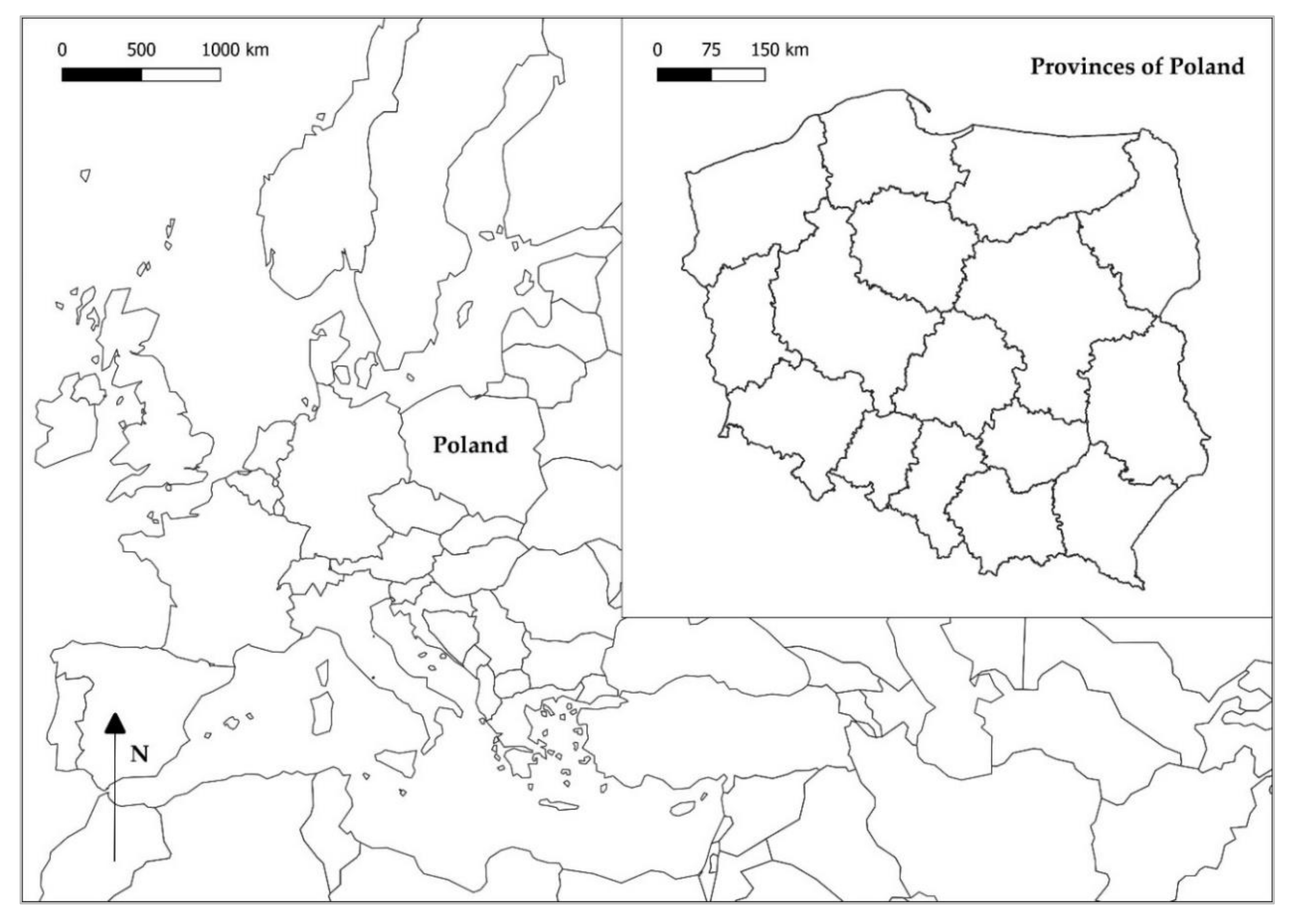
Poland is a country located in central-eastern Europe. The state is divided into communes, counties and provinces. The study area is presented in Figure 1 and concerns all Polish provinces, of which there are currently 16. The dominant form of land use in each voivodship is agricultural land and amounts to 60% of the entire country, emphasising the importance of this study.

2.4. Data—Studying the Convergence

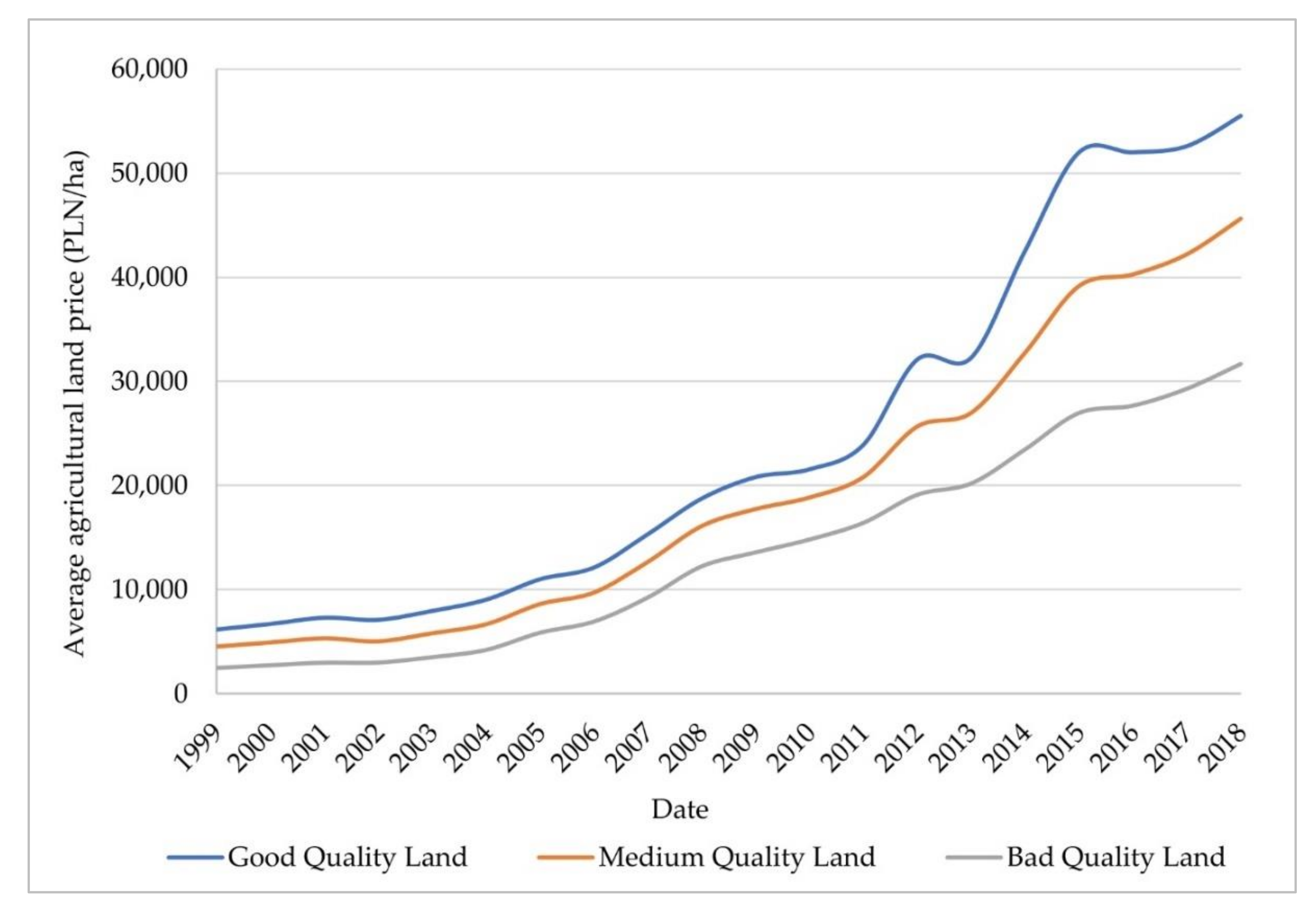
In order to examine agricultural land price convergence, we used yearly data from 1999 to 2018 on the ln-transformed average price of agricultural land per hectare in each Polish province. These data were obtained from Statistics Poland. Moreover, prior to performing the log t regression test, the trend component of the land price series was extracted using two filters. The baseline method is the Hodrick–Prescott [47] filter. This method, however, has been subject to criticism because the production series has spurious dynamic relations. Therefore, another method to extract the trend component is the robust approach outlined by Hamilton [48]. Moreover, as mentioned in the introduction, the convergence examination will be conducted separately for good-quality, medium-quality and bad-quality agricultural land. According to Statistics Poland, good-quality land concerns plots classified by the symbols I, II and IIIa. In turn, medium-quality land is marked by the symbols IIIb, IVa and IVb. The worst land for agricultural purposes includes plots with the symbols V and VI. Furthermore, Statistics Poland offers additional qualifications for the quality of agricultural land. In particular, good-quality land produces wheat and beet, medium-quality land is reserved for rye and potato, and bad-quality land is sandy. It should be noted that on the Polish market there are significant differences in the price of agricultural land of different quality, which are presented in Figure 2. Taking into account the soil quality and average prices eliminates to a large extent the heterogeneity of land and, at the same, allows to investigate the LOP.

2.5. Data—Studying the Driving Forces of the Convergence

Moreover, our study will identify the factors that drive convergence in the entire sample, as well as in the potential identified convergence clubs. Based on the literature review, we selected determinants which may significantly shape the prices of agricultural plots. When selecting the list of independent variables, we focused mainly (but not only) on research on the Polish agricultural land market in order to take into account the specificity of the real estate market in a given country.

The first selected variable describes the value in PLN of agricultural production per hectare of farmland (Agricultural Production) [49,50,51]. This variable presents land productivity [52]; in particular, the Polish statistical office defines it as sum of raw (unprocessed) vegetable and animal products. It should be expected that this variable will have a positive impact on agricultural land prices. It is worth noting that in a sense the analysed variable reflects market fundamentals of farmland prices. This is because the approximation of rents (market fundamentals) is the real agricultural value added [8]. In our case, there is a lack of such data. However, the variable we have adopted is related to the real agricultural value added; in particular, it is the sum of the latter and intermediate consumption.

Another independent variable is share of urbanised land in the total area of a given province (Urbanisation)—very often, in other studies, this variable is expressed in the opposite way, i.e., share of agricultural land in the total area of the territory concerned [50,53]. This variable can be expected to be positively correlated with agricultural land prices. This is due to the fact that urban development increases farmland demand for urban uses, which increases land prices in rural areas [54].

The next explanatory variable concerns the value of gross domestic product per capita (GDP) [49]. This variable presents the general condition of the economy of a given province. It can be expected that the higher GDP per capita the higher prices of agricultural land.

We also decided to include in the model an independent variable describing the average gross monthly salary (Salary). In our opinion, higher wages indicate the higher purchase power of the population [55,56,57], which may lead to increase in agricultural land prices.

Furthermore, as another independent variable we considered the number of pigs per 100 hectares (Pigs) [58]. This variable shows the density of the livestock. It can be assumed that it will be positively correlated with agricultural land prices. This is due to the fact that a higher concentration of livestock increases demand for agricultural land [59].

It should also be noted that agricultural land prices can also be a function of the general level of agricultural commodity prices. A growth of the latter is likely to increase the willingness to pay more for land prices. In order to take account of this dependence, we have constructed a variable (Agricultural Commodity Price) for each province, which reflects the price of a basket of basic agricultural products, in particular: 1 dt wheat, 1 kg slaughter livestock (cattle), 1 kg slaughter livestock (pigs), 1 L cow’s milk.

Prices of agricultural land may also be significantly influenced by the interest rate (Interest Rate). This is due to the fact that low interest rates may affect the willingness to invest in the real estate market due to the reduced attractiveness of bank deposits. Moreover, according to the PV model, agricultural land prices are determined, among other things, by the discount rate [60], which often corresponds to commonly prevailing interest rates [61]. As a result, an increase in the interest rate results in a decrease in the price of agricultural land. Considering the above, a negative correlation between the interest rate and farmland prices should be expected.

Moreover, as indicated in Section 2.2, the set of explanatory variables is supplemented with a lagged dependent variable that reflects land price expectations [62].

Table 1. Average values of independent variables between provinces.

Year	Urbanisation (%)	Salary (PLN)	GDP (PLN)	Agricultural Production (PLN)	Pigs (Units)	Agricultural Commodity Price (PLN)	Interest Rate (%)
2001	4.63	1807.19	18,839.63	2684.21	52.48	58.35	14.5
2002	4.69	2081.07	19,594.13	3387.56	56.96	50.68	8.25
2003	4.83	2147.57	20,423.81	3255.69	55.44	52.39	5.88
2004	4.82	2238.16	22,518.13	3555.13	52.66	56.38	6.00
2005	4.90	2321.60	23,865.00	3930.75	55.98	45.00	5.00
2006	4.96	2439.83	25,755.63	3596.38	55.75	53.04	4.13
2007	4.96	2652.55	28,639.88	3988.50	52.13	78.47	4.63
2008	5.03	2919.96	31,039.63	4744.81	42.26	74.38	5.88
2009	5.09	3054.96	32,584.88	4798.94	42.63	57.56	3.88
2010	5.15	3181.44	34,160.06	4604.75	44.33	68.71	3.50
2011	5.23	3350.54	36,940.19	5238.25	38.83	92.48	4.13
2012	5.30	3471.52	38,343.88	6051.13	32.98	101.60	4.50
2013	5.38	3596.69	39,003.44	6774.31	31.98	92.67	3.13
2014	5.44	3719.73	40,510.19	7363.69	32.94	79.92	2.00
2015	5.51	3857.65	42,353.94	6656.50	30.63	77.46	1.50
2016	5.59	3993.79	43,766.81	6868.13	32.36	73.12	1.50
2017	5.66	4217.73	46,682.06	6741.13	34.45	78.69	1.50
2018	5.71	4497.43	49,567.56	7221.50	31.55	84.57	1.50

Notes: The variable describing the interest rate is global, i.e., it is the same between the surveyed provinces. Moreover, when several levels of interest rate were in force in a given year, a median value is used. Furthermore, in the model specification we used the second-order lagged dependent variable, so there is no need to include in the above table data for period 1999–2000.

presents average values for the defined independent variables.

It should be noted that the above description of variables concerned the determinant used for the estimation of Equation (9). However, in case of empirical verification of the PV model, data on agricultural land rents were obtained from reports entitled “The agricultural land market. Status and prospects”. These reports are issued by the State Institute of Agricultural and Food Economics. On the basis of a review of all reports, data on private agricultural land rental prices are currently only available for the period 2007–2017.

3. Results and Discussion

3.1. Studying Land Price Convergence

The first task of the empirical research was to test for unconditional convergence using the β-convergence model. The results of this analysis indicate that provinces with low initial agricultural land prices are characterised by much higher land price growth rates. This is confirmed by the significant and negative value of the slope parameter from Equation (1), for each type of agricultural land. More specifically, $\beta$ is equal to −0.03, −0.04 and −0.05 for good-quality, medium-quality and bad-quality land, respectively. It should be noted that the β-convergence concept does not reveal anything about the reduction of land price dispersion in the analysed period. Therefore, we performed the σ-convergence test to check how cross-sectional standard deviation of land prices changed over time.

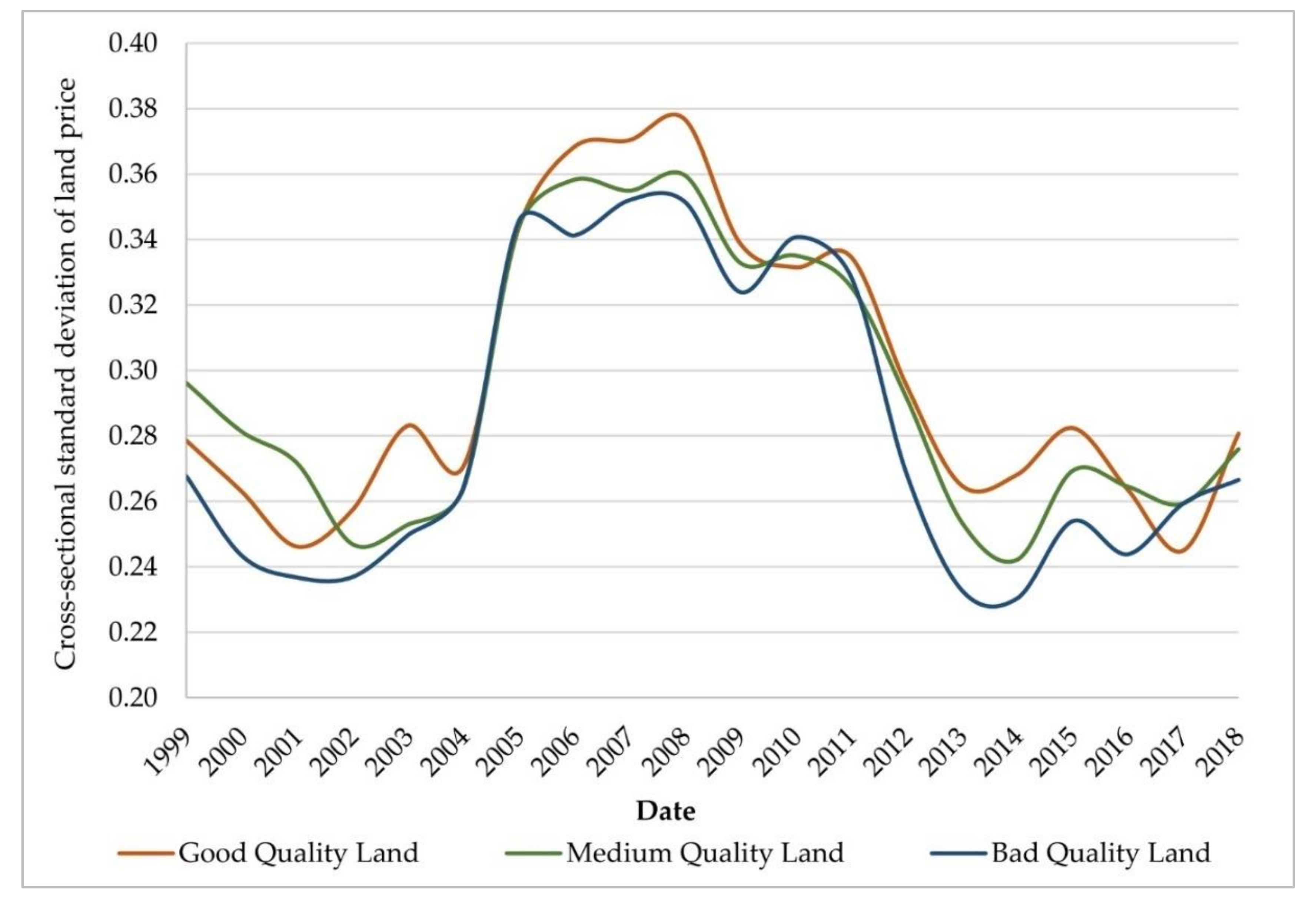
Based on the results of the σ-convergence test presented in Figure 3, one can note an inverted U-shaped pattern for each type of agricultural land. In particular, for the periods 1999–2004 and 2013–2018, we can observe a similar dispersion of land prices. From the years 2005–2012, however, the above-mentioned dispersion skyrocketed (a large variation in agricultural land prices in the above period was also noticed by Czyżewski and Trojanek [63]). This may result from the large fluctuations of world agricultural food prices since 2006, which caused perturbations in many economies [17,64]. The results of the σ-convergence test give little support to the presence of the relative-LOP over the last few years, which can be attributed to the fact that the value of cross-sectional standard deviation of land prices is stable and non-zero. If this value had moved towards zero over time, ultimate convergence would have occurred; hence, the absolute-LOP would have held [65].

Moreover, it should be stressed that the agricultural land market is also part of the real estate market. Therefore, it is of interest to compare it with other segments of the property market. For example, the results of the σ-convergence test for the agricultural land market are entirely different from those observed in the housing market. In particular, a study carried out by Tomal [28] revealed that both in the primary and secondary housing markets one can observe a substantial reduction of house price dispersion in the period 2006–2012, and a slight increase in the following few years. The above emphasise the distinctiveness of the agricultural land market from the rest of the real estate sector.

It should be noted, however, that classical convergence tests have serious shortcomings. On this basis, we performed the log t regression test to an in-depth study of land price convergence across the provinces. The results of this analysis for the entire sample are presented in

Table 2. Log t regression test estimates.

Type of Land	$\widehat{\mathit{b}}$ (HP Filter)	t-Statistic (HP Filter)	$\widehat{\mathit{b}}$ (HAM Filter)	t-Statistic (HAM Filter)
Good-quality Land	−0.1847	−1.5752	0.4224	2.5215
Medium-quality Land	−0.2829 **	−2.5140	0.4640	3.0044
Bad-quality Land	−0.2543 **	−2.0606	0.6404	4.3025

Notes: HP filter—Trend component of time series was extracted using the Hodrick–Prescott filter. HAM filter—Trend component of time series was extracted using the Hamilton filter. Stata software was used to obtain the estimates. ** Five percent level of significance. The number of provinces (N) is 16.

.

Looking at estimates of the log t regression one can conclude that, in relative terms, there is a long-run equilibrium for good-quality land prices. A more complicated situation applies to other types of agricultural land. In particular, this depends on the type of filter used to extract the trend component of land prices. Using the Hodrick–Prescott filter, we can observe that provinces do not share a common trend in the long run for medium and bad-quality land. The log t regression test, however, indicates that there are two sub-groups of provinces, in which land prices converge conditionally, i.e., agricultural land price growth rates tend to converge over time (

Table 3. Convergence clubs according to estimates obtained using the Hodrick–Prescott filter.

Type of Land	Club 1 Provinces	$\widehat{\mathit{b}}$	(t-Statistic)	Club 2 Provinces	$\widehat{\mathit{b}}$	(t-Statistic)
Good-quality Land	16	−0.1847	−1.5752	0	NA	NA
Medium-quality Land	12	0.2259	1.7515	4	1.5659	8.7746
Bad-quality Land	11	0.5579	2.8522	5	1.3886	5.1730

Note: the results indicate that the speed of convergence is much higher in clubs 2 ($\widehat{\alpha }=\widehat{b}/2=0.78$or $\widehat{\alpha }=\widehat{b}/2=0.69$ , for medium and bad-quality land respectively). Medium quality land—club 1: Greater Poland, Kuyavian-Pomeranian, Lower Silesian, Lubusz, Masovian, Opole, Podlaskie, Pomeranian, Silesian, Warmian-Masurian, West Pomeranian, Łódź. Medium-quality land—club 2: Holy Cross, Lesser Poland, Lublin, Subcarpathian. Bad quality land—club 1: Greater Poland, Kuyavian-Pomeranian, Lower Silesian, Lubusz, Masovian, Opole, Podlaskie, Pomeranian, Warmian-Masurian, West Pomeranian, Łódź. Bad quality land—club 2: Holy Cross, Lesser Poland, Lublin, Subcarpathian, Silesian. Stata software was used to obtain the estimates.

).

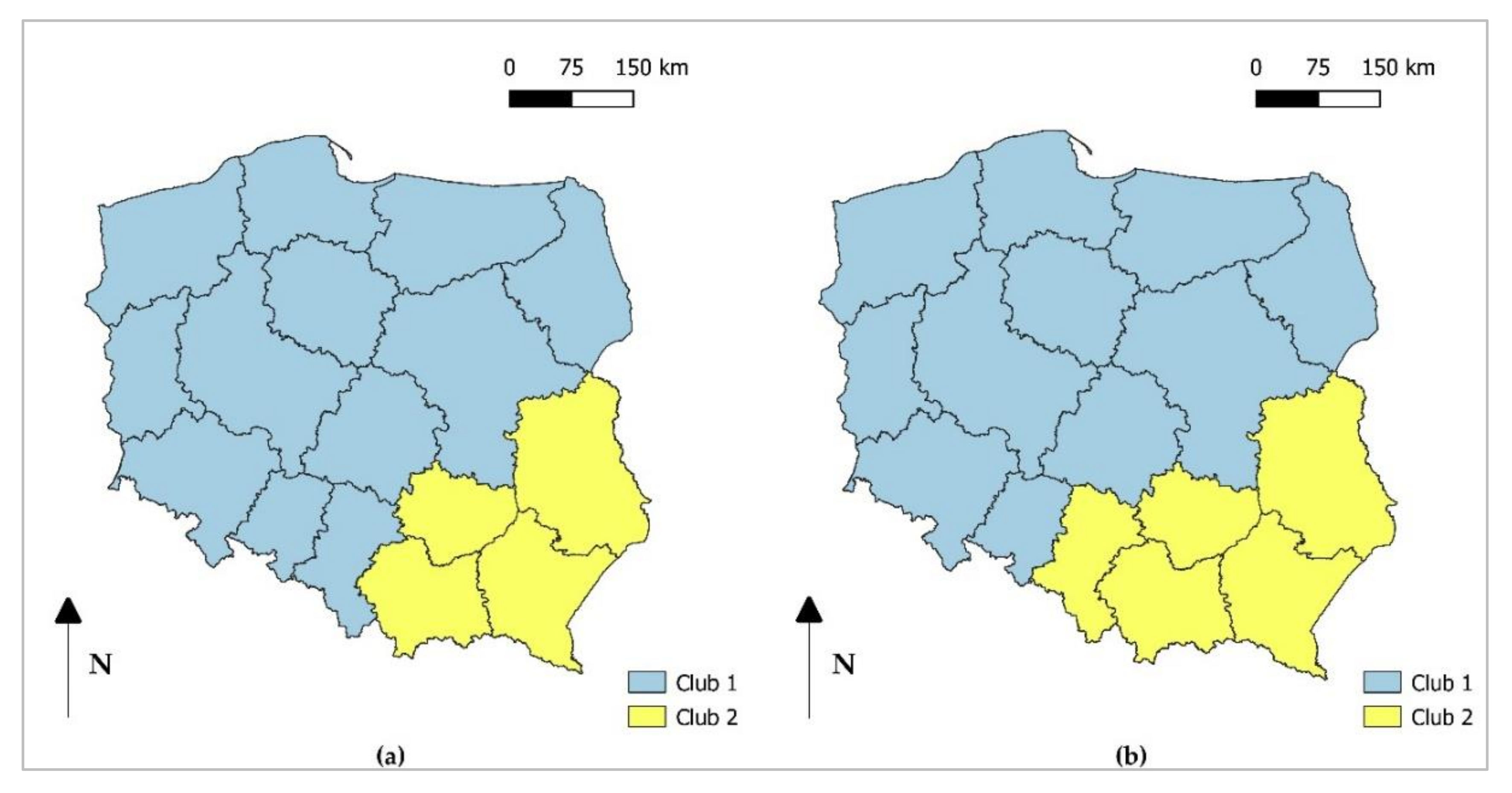
As can be seen in Figure 4a,b, convergence clubs are closely linked in space. Both for medium and bad-quality land, the first club covers the central, western and northern parts of the country, while the second contains provinces located in the south-eastern area of Poland. The latter is consistent with studies conducted by Chrzanowska [66]. It should also be stressed that the existence of such rather than other convergence clubs may result from similar production characteristics of agriculture in the identified areas and from a significantly different fragmentation of agricultural holdings. A detailed comparison can be found in

Table 4. Comparison of the convergence clubs.

Variable	Club 1	Club 2
Average farm size (ha)	15.0	5.7
Labour productivity (PLN)	70,519.1	24,412.9
Degree of commodity (%)	95.6	88.8
Land productivity per hectare of farmland (PLN)	7081.4	7529.8

Notes: Labour productivity is defined as ratio of land productivity and the number of people working in agriculture. Degree of commodity means the share of commodity production in final production. For comparison purposes, convergence clubs identified for bad-quality land were selected.

.

Conversely, the results of the log t regression test using the Hamilton filter indicate a different outcome. In particular, there is strong evidence that all time series tend to converge, which means that all provinces in Poland create one large convergence club, sharing a common trend in the long run. This finding is much more reliable, taking into account that the Hamilton filter is a robust approach for extracting a trend component of the time series. It should be mentioned, however, that the above interpretation concerns convergence in relative terms (growth convergence). Therefore, there is no evidence that agricultural land prices across the provinces head to a single price level.

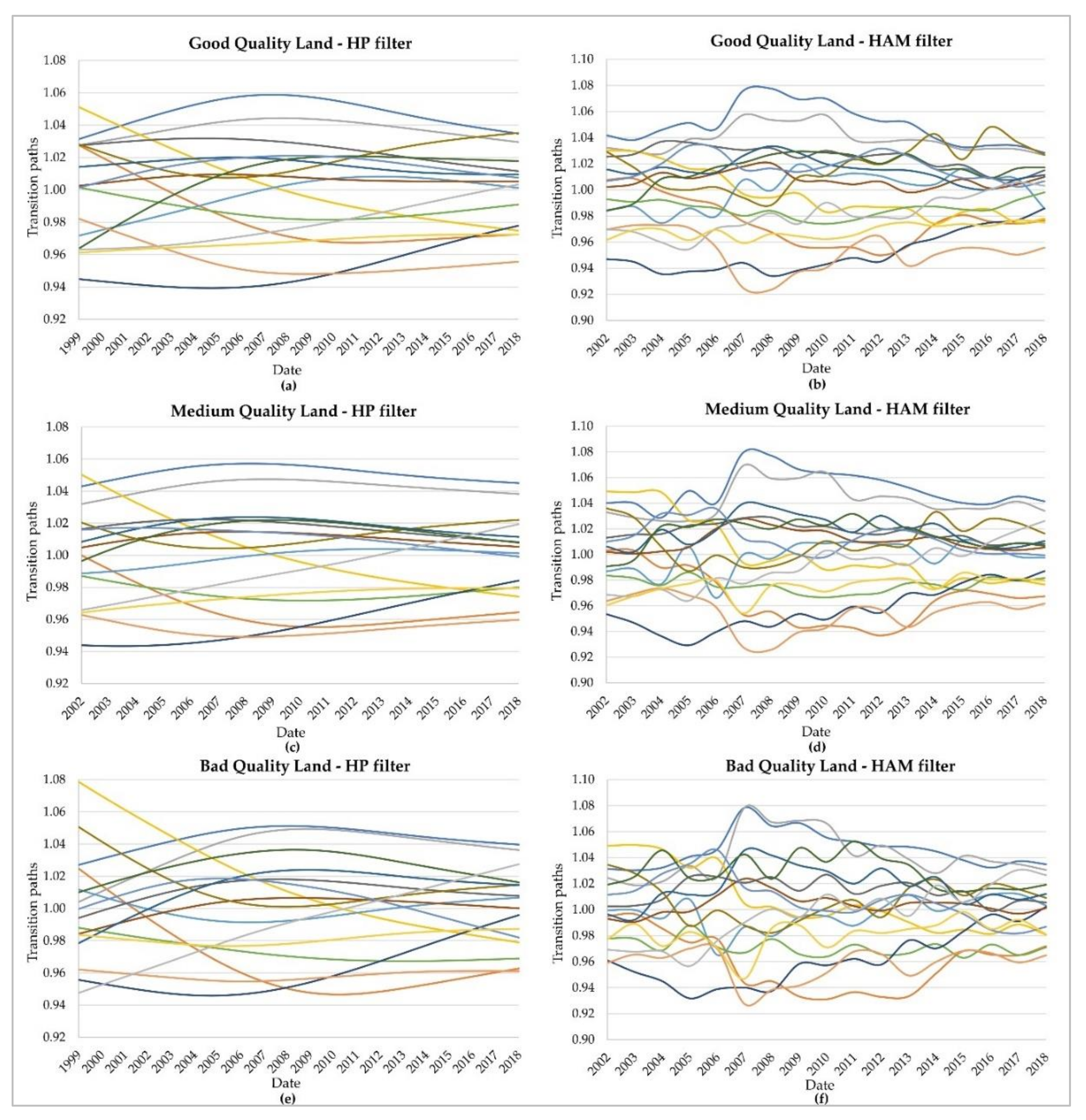
It is also of interest to analyse relative transition paths. In particular, Figure 5a–e reveals the existing cross-sectional and time-series heterogeneity in the data. Therefore, convergence tests that take into consideration the assumption of homogeneous individuals (provinces, cities, etc.) are not suitable for studying the convergence of real estate prices. The transition curves can reveal more patterns. In particular, each panel in Figure 5 indicates that in the years 1999–2007/08, agricultural land prices across the provinces tended to diverge from the panel average. Particularly strong land price volatility has been evident in the final years of the period mentioned above. This may be due, among other things, to the large fluctuations in agricultural commodity markets, but also to the 2008 financial crisis, which had a very large impact on the functioning of the real estate market [67,68]. In subsequent years (2009–2018), however, agricultural land prices across provinces were characterised by “catching-up”, i.e., prices moving towards the panel average ($h_{it}\to 1$ for all $i$, as $t\to \infty$). These findings are very important for Polish policy-makers, who in 2016 enacted new laws that greatly limited the possibility of purchasing farmland by non-agricultural agents [69]. Furthermore, the sale of state-owned agricultural land larger than two hectares was halted for a period of five years. All this was aimed at limiting the “speculative” buyout of agricultural land, guaranteeing its agricultural use. After the introduction of such laws, many experts believed that turnover on the agricultural real estate market would fall significantly, leading to a strong price collapse. Following the introduction of the new regulations, however, as our study indicates, agricultural land prices stagnated and then began to rise (Figure 2), which is in line with other research [2]. Moreover, the tightening of the rules has not affected price convergence processes, as clearly presented in Figure 5a–e. However, it should be stressed that the above conclusions are only drawn on the basis of data covering two full years after the change in the agricultural land policy. Moreover, our analysis does not examine how the price dynamics would have behaved if the above mentioned amendment of the law had not entered into force. Therefore, in order to fully assess the impact of the new law, the process of spatial integration of the agricultural land market needs to be further studied.

Summarising the results of testing convergence using the log t regression, it should be stated that, generally, agricultural land prices in Poland tend to converge in the long run in relative terms. Some premises for the existence of convergence clubs for both medium and bad-quality land markets can be observed. These, however, can be largely questioned because they result from the application of a non-robust method to extract trend components from time series.

3.2. Studying the Driving Forces of Convergence

The final task of the empirical research was to examine which factors drive the convergence of agricultural land prices across studied provinces. Firstly, using the methodology outlined in Section 2.2, we have selected the proper panel data model and then we tested for the presence of cross-sectional dependence in our data (

Table 5. Hausman, Paseran and Breusch-Pagan tests estimates.

Type of Land	Hausman	Pesaran	Breusch-Pagan
Good-quality Land	75.13 ***	14.78 ***	325.02 ***
Medium-quality Land	63.66 ***	13.14 ***	332.78 ***
Bad-quality Land	58.00 ***	10.96 ***	282.02 ***

Notes: *** One percent level of significance. For the Hausman test statistical significance indicates a need to apply a fixed effects model. For Pesaran and Breusch-Pagan tests statistical significance indicates the presence of cross-sectional dependence.

).

Finally, based on results of the Hausman, Paseran and Breusch–Pagan tests we estimated three dynamic fixed effects models with corrected standard errors using the Driscoll and Kraay approach to account for cross-sectional dependence.

The results presented in

Table 6. Dynamic fixed effects model with Driscoll and Kraay standard errors estimates.

Variable	Good-Quality Land	Medium-Quality Land	Bad-Quality Land
$\ln p_{i,t-1}$	0.8374 ***	0.9559 ***	0.9875 ***
$\ln p_{i,t-2}$	−0.1436	−0.2501 ***	−0.2756 ***
Urbanisation	−0.3832 *** (−1.25)	−0.4259 *** (−1.45)	−0.5382 *** (−1.87)
Salary	−0.2194 (−0.72)	−0.0654 (−0.22)	0.0835 (0.29)
Agricultural Production	0.1482 (0.48)	0.1237 (0.42)	0.1152 (0.40)
GDP	0.3883 ** (1.27)	0.3544 * (1.20)	0.4138 ** (1.44)
Pigs	−0.0132 (−0.04)	0.0437 (0.15)	0.0886 ** (0.31)
Agricultural Commodity Price	0.2594 *** (0.85)	0.2525 ** (0.86)	0.2065 * (0.72)
Interest Rate	−0.1417 ** (−0.46)	−0.1139 ** (−0.39)	−0.0820 * (−0.28)
$R^2$	0.9850	0.9860	0.9844

Notes: *** One percent level of significance. ** Five percent level of significance. * Ten percent level of significance. Stata software was used to obtain the estimates. Estimates represents short-run elasticities and in the parenthesis log-term ones. The number of provinces (N) is 16.

indicate that the selected models explain to a large extent the volatility of agricultural land prices, i.e., the coefficient of determination $R^2$ in each model oscillated around 98%.

The estimated relationships between the variables largely agree with the theoretical considerations presented in Section 2.5. In particular, the variable describing GDP per capita has the strongest impact on agricultural land prices. In the long term, an increase of the latter by 1% leads to an increase in the price of agricultural land by 1.27%, 1.20% and 1.44% for good-quality, medium-quality and bad-quality land, respectively. Taking into account the above mentioned results, it should be stated that the general economic condition in a given province has a very big influence on farmland prices. A stable and positive relationship can also be observed between prices of agricultural products and the dependent variable. It should be noted that agricultural land prices largely imitate movements in the analysed independent variable. In this respect, however, some differences can be observed in terms of the quality of agricultural land. For good and medium-quality land in particular, a 1% increase in agricultural product prices results in an increase of the dependent variable by about 0.85%. On the other hand, for bad-quality land this increase amounts to 0.72%, which results from the fact that this type of agricultural land is characterized by a low level of productivity. The last independent variable, which has a positive impact on the current price of agricultural land of all qualities, reflects farmland price expectations. Furthermore, only for bad-quality land was the significant impact of livestock density on the dependent variable observed. This is due to the fact that in Poland, but also in other countries, there are legal provisions on the maximum livestock density per hectare. Therefore, an increase in livestock density will generate an increase in demand for mainly lower quality agricultural land, as there is no need to buy higher-quality land.

In turn, a negative correlation between the degree of interest rate and the price of agricultural land is visible. This result is also in line with expectations, as the lower interest rate increases the attractiveness of investing in real estate. The variable concerning the degree of urbanization also has a negative impact on the dependent variable. This relationship is the only one that does not agree with theoretical considerations. However, this relationship is characterised by a high degree of statistical significance in relation to agricultural land of all qualities. Therefore, this unexpected impact should be further investigated.

On the other hand, an insignificant impact on agricultural land prices concerns the variables describing the level of wages and agricultural production. In the context of the first case, this situation may result from the significance of the variable characterising GDP per capita. On the other hand, it is surprising that the latter has no significant impact on prices. This is an unfavourable situation from the point of view of the efficiency level of agricultural land market in Poland, because this variable, from the theoretical point of view, is closely related to the main proxy of market fundamentals.

The above finding led us to carry out a direct assessment of the impact of market fundamentals (rents) on farmland prices, in particular we employed the present value model by regressing agricultural land price per hectare on rent per hectare. The results obtained indicated that farmland prices do not mimic movements in rents with an elasticity equal to one in the long run (

Table 7. Elasticity of agricultural land prices with respect to rents in years 2007–2017.

Type of Land	Elasticity in the Long-Run
Good-quality Land	1.24 ***
Medium-quality Land	0.75 ***
Bad-quality Land	0.70 ***

Notes: Estimates based on dynamic fixed effects model with Driscoll and Kraay standard errors. *** One percent level of significance. The number of provinces (N) is 16.

), which may be due to the fact that also other factors determine the market price of land and not only the present value measure [8]. The latter hypothesis has also been proven in this study (Table 6) and by other researchers. One can mention here a study carried out by Delbecq et al. [70], which showed that prices of agricultural land are only partially explained by farmland rents. Therefore, the empirical application of the present value model ultimately proved that the agricultural land sales market in Poland cannot be regarded as efficient.

When analysing the results presented in Table 7 in detail, it should be noted that for a good-quality land, rents are rising at a slower rate than land prices. Excessively high levels of the latter may result in the agricultural land not being effectively redistributed, i.e., only farmers with sufficient financial resources will be able to afford to buy land at a price that does not reflect its fundamental value. The situation is different for medium- and bad-quality lands, where land prices are far below their fundamental values. This may herald too high a level of rents, which may lead to unprofitable agricultural production. Extremely high levels of rents for agricultural land were reported by the Chamber of Agriculture in Poland in 2016. Illegal sources of funds from which rents were financed were indicated as one of the reasons. The findings obtained as a result of estimating the PV model should be taken with great caution. This is due to the fact that the survey was conducted only for the years 2007-2017 due to the lack of data for the remaining years in terms of rents. In addition, there is still a grey area of rentals in Poland. Additionally, a large proportion of actually concluded contracts are not properly recorded anywhere.

4. Conclusions

In this study, we addressed for the first time in the scientific literature the problem of efficiency of the agricultural land sales market in Poland using the concept of spatial market integration as well as the PV model. Empirically, the convergence processes of agricultural land prices were evaluated using three different methods. In particular, the results of the log t regression test showed that the prices of agricultural land across the provinces share a common long-term growth path. This conclusion is universal for good-, medium- and bad-quality land. Taking into account this finding and estimates from β- and σ-convergence tests, one can conclude that integration in the Polish agricultural land market is increasing. There is not enough evidence, however, to infer that the absolute version of the LOP holds. This conclusion can be explained by the fact that the land is immobile and an extremely heterogeneous good, which makes convergence very slow in this case. In addition, the significant variation in agricultural land prices between provinces can be justified on the basis of the theory of the new geography economy, according to which forces such as economies of scale or knowledge spillovers may foster the geographical concentration of economic activities [71]. In this instance, the occurrence of high prices of agricultural land may constitute a blocking force for further concentration of agricultural production, whose excessive level, according to Yang at al. [7], may negatively affect the environment.

Moreover, extremely interesting findings stem from the results of the σ-convergence model. In particular, in the analysed period, the cross-sectional standard deviation of agricultural land prices adopts an inverse U-shaped pattern. Furthermore, the drivers behind the convergence of the studied prices were examined. In this respect, using dynamic fixed effects models, it was identified that for good-, medium- and bad-quality land prices almost the same drivers of convergence apply. The only differences concern the strength of the influence of independent variables on prices of farmland of various types. Additionally, bad-quality land prices are the only ones which are affected by livestock density. Moreover, estimates of the present value (PV) model proved that farmland prices do not mimic changes in rents with a long-term elasticity equal to one, which finally confirmed that agricultural land sales market in Poland cannot be considered as efficient.

This study has certain limitations. First of all, guided by the availability of price information, entire provinces were analysed. Future studies could focus on smaller areas, such as municipalities or counties, because the real estate market is local and heterogeneous in nature. Secondly, if relevant data were available, it would be worthwhile to carry out a study taking into account longer time series of agricultural land prices, which would certainly increase the robustness of the survey. Moreover, this study attempted to analyse relatively homogeneous goods, i.e., agricultural land of different quality. As indicated in Section 2.4, this division in each dimension includes agricultural land of several valuation classes. Therefore, future analyses could examine more homogeneous goods, e.g., agricultural land of class 1 only, etc. Furthermore, the validity of the relative version of the LOP on the Polish agricultural land sale market requires further investigation. To this end, future studies could use panel unit root tests, which can detect whether time series (for example land prices) converge to a constant difference [72]. Finally, in our study, we did not have rental data for the full period under study, which reduces the reliability of the PV model results.

Our analysis is very important for policy-makers and agricultural land management in Poland. It should be noted that this study mainly concerned the period before the introduction of the law limiting trade in agricultural land, which took place in 2016. The results obtained indicated that at that time the agricultural land market was not efficient. Therefore, it can be concluded that there was a certain basis for changing the legal regulations. However, currently it is not possible to make an accurate assessment of the imposed restrictions. Therefore, research on the functioning of the agricultural land market in Poland should be continued, because efficient agriculture is crucial not only for farmers, but also, as Salim et al. note [73], for sustainable development of a country due to the broad connection between agriculture and the rest of the economy [74].

References

- Hubacek, K.; Fischer, G. The Role of Land in Economic Theory; International Institute for Applied Systems Analysis (IIASA): Laxenburg, Austria, 2002; pp. 1–48. [Google Scholar]
- Gołębiewska, B.; Stefańczyk, J. Zmiany cen gruntów rolnych w Polsce po wejściu w życie nowej ustawy o kształtowaniu ustroju rolnego. Rocz. Nauk. Stowarzyszenia Ekon. Rol. Agrobiz. 2016, 18, 29–34. [Google Scholar]
- Qiang, W.; Niu, S.; Liu, A.; Kastner, T.; Bie, Q.; Wang, X.; Cheng, S. Trends in global virtual land trade in relation to agricultural products. Land Use Policy 2020, 92, 104439. [Google Scholar] [CrossRef]
- Firlej, K. Rozwój Przemysłu Rolno-Spożywczego w Sektorze Agrobiznesu i Jego Determinanty; Wydawnictwo Uniwersytetu Ekonomicznego w Krakowie: Krakow, Poland, 2008. [Google Scholar]
- Yang, X.; Odening, M.; Ritter, M. The Spatial and Temporal Diffusion of Agricultural Land Prices. Land Econ. 2019, 95, 108–123. [Google Scholar] [CrossRef] [Green Version]
- Grau, A.; Odening, M.; Ritter, M. Land price diffusion across borders—The case of Germany. Appl. Econ. 2019, 1–18. [Google Scholar] [CrossRef]
- Yang, X.; Ritter, M.; Odening, M. Testing for regional convergence of agricultural land prices. Land Use Policy 2017, 64, 64–75. [Google Scholar] [CrossRef]
- Carmona, J.; Roses, J.R. Land markets and agrarian backwardness (Spain, 1904–1934). Eur. Rev. Econ. Hist. 2012, 16, 74–96. [Google Scholar] [CrossRef] [Green Version]
- Thomson, D.N.; Lyne, M.C. A land rental market in Kwazulu: Implications for farming efficiency. Agrekon 1991, 30, 287–290. [Google Scholar] [CrossRef] [Green Version]
- Engsted, T. Do farmland prices reflect rationally expected future rents? Appl. Econ. Lett. 1998, 5, 75–79. [Google Scholar] [CrossRef]
- Czyżewski, B.; Kułyk, P.; Kryszak, Ł. Drivers for farmland value revisited: Adapting the returns discount model (RDM) to the sustainable paradigm. Econ. Res. Ekon. Istraživanja 2019, 32, 2080–2098. [Google Scholar] [CrossRef] [Green Version]
- Tegene, A.; Kuchler, F.R. Evidence on the existence of speculative bubbles in farmland prices. J. Real Estate Finan. Econ. 1993, 6, 223–236. [Google Scholar] [CrossRef]
- Cirera, X.; Arndt, C. Measuring the impact of road rehabilitation on spatial market efficiency in maize markets in Mozambique. Agric. Econ. 2008, 39, 17–28. [Google Scholar] [CrossRef] [Green Version]
- Cherevyk, D.; Hamulczuk, M. Ukraiński rynek kukurydzy na tle zmian światowych. Zesz. Nauk. SGGW Warszawie Probl. Rol. Światowego 2018, 18, 33–43. [Google Scholar] [CrossRef] [Green Version]
- Goldberg, P.K.; Verboven, F. Market integration and convergence to the Law of One Price: Evidence from the European car market. J. Int. Econ. 2005, 65, 49–73. [Google Scholar] [CrossRef] [Green Version]
- Goodwin, B.K.; Piggott, N.E. Spatial Market Integration in the Presence of Threshold Effects. Am. J. Agric. Econ. 2001, 83, 302–317. [Google Scholar] [CrossRef] [Green Version]
- Hamulczuk, M.; Makarchuk, O.; Sica, E. Price Behaviour and Market Integration: Preliminary Evidencefrom the Ukrainian and European Union Rapeseed Markets. Zesz. Nauk. SGGW Warszawie Probl. Rol. Światowego 2019, 19, 47–58. [Google Scholar] [CrossRef]
- Waights, S. Does the law of one price hold for hedonic prices? Urban Stud. 2018, 55, 3299–3317. [Google Scholar] [CrossRef]
- Twardowska, A. Konwergencja typu sigma cen gruntów rolnych w państwach Unii Europejskiej. Zesz. Nauk. SGGW Warszawie Probl. Rol. Światowego 2019, 19, 133–143. [Google Scholar] [CrossRef] [Green Version]
- Wyrzykowski, P. Konwergencja cen żywności w Unii Europejskiej. Rocz. Nauk. Stowarzyszenia Ekon. Rol. Agrobiz. 2015, 17, 356–361. [Google Scholar]
- Zawojska, A. Zróżnicowanie i konwergencja cen dóbr konsumpcyjnych w integrującej się Europie. Rocz. Ekon. Rol. Rozw. Obsz. Wiej. 2012, 99, 16–32. [Google Scholar]
- Roman, M. Spatial Integration of the Milk Market in Poland. Sustainability 2020, 12, 1471. [Google Scholar] [CrossRef] [Green Version]
- Nalepka, A.; Tomal, M. Identyfikacja czynników kształtujących ceny ofertowe deweloperskich lokali mieszkalnych na obszarze jednostki ewidencyjnej Nowa Huta. Świat Nieruchom. 2016, 11–18. [Google Scholar] [CrossRef]
- Małkowska, A.; Uhruska, M.; Tomal, M. Age and Experience versus Susceptibility to Client Pressure among Property Valuation Professionals—Implications for Rethinking Institutional Framework. Sustainability 2019, 11, 6759. [Google Scholar] [CrossRef] [Green Version]
- Głuszak, M.; Marona, B. Heterogeneity and clustering of housing demand: Case study. J. Int. Stud. 2011, 4, 89–97. [Google Scholar] [CrossRef] [PubMed]
- Phillips, P.C.B.; Sul, D. Transition Modeling and Econometric Convergence Tests. Econometrica 2007, 75, 1771–1855. [Google Scholar] [CrossRef] [Green Version]
- Phillips, P.C.B.; Sul, D. Economic transition and growth. J. Appl. Econ. 2009, 24, 1153–1185. [Google Scholar] [CrossRef] [Green Version]
- Tomal, M. House Price Convergence on the Primary and Secondary Markets: Evidence from Polish Provincial Capitals. Real Estate Manag. Valuat. 2019, 27, 62–73. [Google Scholar] [CrossRef] [Green Version]
- Young, A.T.; Higgins, M.J.; Levy, D. Sigma Convergence versus Beta Convergence: Evidence from U.S. County-Level Data. J. Money Credit Bank. 2008, 40, 1083–1093. [Google Scholar] [CrossRef]
- Bai, C.; Mao, Y.; Gong, Y.; Feng, C. Club Convergence and Factors of Per Capita Transportation Carbon Emissions in China. Sustainability 2019, 11, 539. [Google Scholar] [CrossRef] [Green Version]
- Matysiak, G.; Olszewski, K. A panel analysis of Polish regional cities: Residential price convergence in the primary market. NBP Work. Pap. 2019, 316, 1–39. [Google Scholar] [CrossRef] [Green Version]
- Du, K. Econometric convergence test and club clustering using Stata. Stata J. 2017, 882–900. [Google Scholar] [CrossRef]
- Kim, Y.S.; Rous, J.J. House price convergence: Evidence from US state and metropolitan area panels. J. Hous. Econ. 2012, 21, 169–186. [Google Scholar] [CrossRef]
- Schnurbus, J.; Haupt, H.; Meier, V. Economic Transition and Growth: A Replication. J. Appl. Econom. 2017, 32, 1039–1042. [Google Scholar] [CrossRef]
- Choi, C.-Y.; Wang, X. Discontinuity of output convergence within the united states: Why has the course changed? Econ. Inq. 2015, 53, 49–71. [Google Scholar] [CrossRef]
- Borsi, M.T.; Metiu, N. The evolution of economic convergence in the European Union. Empir. Econ. 2015, 48, 657–681. [Google Scholar] [CrossRef]
- Blanco, F.; Delgado, F.; Presno, M. R&D expenditure in the EU: Convergence or divergence? Econ. Res. 2020, 33, 1685–1710. [Google Scholar] [CrossRef]
- Wang, S.; Yang, Z.; Liu, H. Impact of urban economic openness on real estate prices: Evidence from thirty-five cities in China. China Econ. Rev. 2011, 22, 42–54. [Google Scholar] [CrossRef]
- Li, Q.; Chand, S. House prices and market fundamentals in urban China. Habitat Int. 2013, 40, 148–153. [Google Scholar] [CrossRef]
- Greene, W.H. Econometric Analysis, 8th ed.; Pearson: New York, NY, USA, 2018. [Google Scholar]
- Galvao, A.F. Quantile regression for dynamic panel data with fixed effects. J. Econom. 2011, 164, 142–157. [Google Scholar] [CrossRef]
- Zhu, H.; Li, Z.; Guo, P. The impact of income, economic openness and interest rates on housing prices in China: Evidence from dynamic panel quantile regression. Appl. Econ. 2018, 50, 4086–4098. [Google Scholar] [CrossRef]
- Hausman, J.A. Specification Tests in Econometrics. Econometrica 1978, 46, 1251. [Google Scholar] [CrossRef] [Green Version]
- Pesaran, M.H. General Diagnostic Tests for Cross Section Dependence in Panels; Faculty of Economics, University of Cambridge: Cambridge, UK, 2004; CWPE0435. [Google Scholar] [CrossRef]
- Breusch, T.S.; Pagan, A.R. The Lagrange Multiplier Test and its Applications to Model Specification in Econometrics. Rev. Econ. Stud. 1980, 47, 239. [Google Scholar] [CrossRef]
- Driscoll, J.C.; Kraay, A.C. Consistent Covariance Matrix Estimation with Spatially Dependent Panel Data. Rev. Econ. Stat. 1998, 80, 549–560. [Google Scholar] [CrossRef]
- Hodrick, R.J.; Prescott, E.C. Postwar U.S. Business Cycles: An Empirical Investigation. J. Money Credit Bank. 1997, 29, 1. [Google Scholar] [CrossRef]
- Hamilton, J.D. Why You Should Never Use the Hodrick-Prescott Filter. Rev. Econ. Stat. 2018, 100, 831–843. [Google Scholar] [CrossRef]
- Firlej, K.; Kubala, S. Ceny ziemi rolnej w Polsce na tle Unii Europejskiej. Zesz. Nauk. UEK 2018, 159–171. [Google Scholar] [CrossRef]
- Kuźmiński, W. Ekonometryczny model cen gruntów rolnych. Studia Pr. WNEiZ 2015, 42, 227–240. [Google Scholar] [CrossRef] [Green Version]
- Lovrinčević, Ž.; Vizek, M. Agricultural land in the new EU member states and Croatia: Prices, affordabilities and convergence potential. Ekon. Pregl. 2009, 60, 28–49. [Google Scholar]
- Kulikowski, R. Produktywność i towarowość rolnictwa w Polsce. Rozw. Reg. Polityka Reg. 2014, 95. [Google Scholar] [CrossRef] [Green Version]
- Kocur-Bera, K. Determinants of agricultural land price in Poland—A case study covering a part of the Euroregion Baltic. Cah. Agric. 2016, 25, 25004. [Google Scholar] [CrossRef] [Green Version]
- Livanis, G.; Moss, C.B.; Breneman, V.E.; Nehring, R.F. Urban Sprawl and Farmland Prices. Am. J. Agric. Econ. 2006, 88, 915–929. [Google Scholar] [CrossRef]
- Tomal, M. The Impact of Macro Factors on Apartment Prices in Polish Counties: A Two-Stage Quantile Spatial Regression Approach. Real Estate Manag. Valuat. 2019, 27, 1–14. [Google Scholar] [CrossRef] [Green Version]
- Tomal, M. Moving towards a Smarter Housing Market: The Example of Poland. Sustainability 2020, 12, 683. [Google Scholar] [CrossRef] [Green Version]
- Nowak, K. Ceny mieszkań a wynagrodzenie i bezrobocie—Analiza z wykorzystaniem modeli wektorowo--autoregresyjnych na przykładzie Krakowa. Probl. Rozw. Miast 2014, 4, 20–33. [Google Scholar]
- Drescher, K.; McNamara, K.T. Determinants of German farmland prices. In ERSA Conference Papers, Proceedings of the 39th Congress of the European Regional Science Association, Dublin, Ireland, 23–27 August, 1999; European Regional Science Association (ERSA): Dublin, Ireland, 1999. [Google Scholar]
- Breustedt, G.; Habermann, H. The Incidence of EU Per-Hectare Payments on Farmland Rental Rates: A Spatial Econometric Analysis of German Farm-Level Data: Incidence of EU Per-Hectare Payments on Farmland Rental Rates. J. Agric. Econ. 2011, 62, 225–243. [Google Scholar] [CrossRef] [Green Version]
- Gloy, B.A.; Boehlje, M.; Dobbins, C.L.; Hurt, C.; Baker, T.G. Are economic fundamentals driving farmland values? Choices 2011, 26, 1–6. [Google Scholar] [CrossRef]
- Sherrick, B.J. Understanding Farmland Values in a Changing Interest Rate Environment. Choices 2018, 33, 1–8. [Google Scholar] [CrossRef]
- Gluszak, M. Expectations and House Prices: An Exploratory Analysis. World Real Estate J. 2019, 4, 15–28. [Google Scholar] [CrossRef]
- Czyżewski, B.; Trojanek, R. Czynniki wartości ziemi rolnej w kontekście zróżnicowanych funkcji obszarów wiejskich w Polsce. Zagadnienia Ekon. Rolnej 2016, 347, 3–25. [Google Scholar] [CrossRef] [Green Version]
- Bellemare, M.F. Rising Food Prices, Food Price Volatility, and Social Unrest. Am. J. Agric. Econ. 2015, 97, 1–21. [Google Scholar] [CrossRef] [Green Version]
- Fousekis, P. Convergence of Relative State-level Per Capita Incomes in the United States Revisited. J. Reg. Anal. Policy 2007, 37, 80–89. [Google Scholar]
- Chrzanowska, M. Spatial analysis of agricultural land prices by regions in Poland. Econ. Sci. Rural Dev. 2016, 42, 30–37. [Google Scholar]
- Batóg, B.; Foryś, I. Structural Changes on Polish Housing Market: Has the Market Returned to the Level Before the Crisis? In Eurasian Economic Perspectives, Proceedings of the 25th Eurasia Business and Economics Society Conference, Berlin, Germany, 23–25 May 2018; Bilgin, M.H., Danis, H., Karabulut, G., Gözgor, G., Eds.; Springer International Publishing: Cham, Switzerland, 2020; pp. 55–69. [Google Scholar]
- Brzezicka, J.; Laszek, J.; Olszewski, K. An Analysis of the Relationships Between Domestic Real Estate Markets–A Systemic Approach. Real Estate Manag. Valuat. 2019, 27, 79–91. [Google Scholar] [CrossRef] [Green Version]
- Czyzewski, B.; Trojanek, R.; Matuszczak, A. The effects of use values, amenities and payments for public goods on farmland prices: Evidence from Poland. Acta Oeconomica 2018, 68, 135–158. [Google Scholar] [CrossRef]
- Delbecq, B.A.; Kuethe, T.H.; Borchers, A.M. Identifying the Extent of the Urban Fringe and Its Impact on Agricultural Land Values. Land Econ. 2014, 90, 587–600. [Google Scholar] [CrossRef]
- Schmutzler, A. The New Economic Geography. J. Econ. Surv. 1999, 13, 355–379. [Google Scholar] [CrossRef] [Green Version]
- Liu, L.; Ruiz, I. Convergence Hypothesis: Evidence from Panel Unit Root Test with Spatial Dependence. Ecos Econ. Lat. Am. J. Appl. Econ. 2006, 10, 37–56. [Google Scholar]
- Salim, R.; Hassan, K.; Rahman, S. Impact of R&D expenditures, rainfall and temperature variations in agricultural productivity: Empirical evidence from Bangladesh. Appl. Econ. 2019, 1–14. [Google Scholar] [CrossRef]
- Oladosu, G. Economic Impacts of Potential Foot and Mouth Disease Agroterrorism in the USA: A General Equilibrium Analysis. J. Bioterror. Biodef. 2012, s12. [Google Scholar] [CrossRef] [Green Version]
Figure 1.
The study area.
Figure 2.
Average agricultural land prices (PLN/ha) in Poland in the years 1999–2018.
Figure 3.
Results of the σ-convergence test in the years 1999–2018. Note: land prices are ln-transformed.
Figure 4.
(a) Convergence clubs for medium-quality land. (b) Convergence clubs for bad-quality land. Note: estimates using the Hodrick–Prescott filter. Stata and QGis software was used to obtain the estimates.
Figure 5.
(a) Estimates of transition paths for good-quality land using the Hodrick–Prescott filter. (b) Estimates of transition paths for good-quality land using the Hamilton filter. (c) Estimates of transition paths for medium-quality land using the Hodrick–Prescott filter. (d) Estimates of transition paths for medium-quality land using the Hamilton filter. (e) Estimates of transition paths for bad-quality land using the Hodrick–Prescott filter. (f) Estimates of transition paths for bad-quality land using the Hamilton filter. Notes: there are sixteen transition paths representing all provinces in Poland in each panel above. Convergence exists when all curves tend to narrow toward unity. Stata software was used to obtain the estimates.