Online Identification-Verification-Prediction Method for Parallel System Control of UAVs

Abstract

In order to solve the problem of how to efficiently control a large-scale swarm Unmanned Aerial Vehicle (UAV) system, which performs complex tasks with limited manpower in a non-ideal environment, this paper proposes a parallel UAV swarm control method. The key technology of parallel control is to establish a one-to-one artificial UAV system corresponding to the aerial swarm UAV on the ground. This paper focuses on the computational experiments algorithm for artificial UAV system establishment, including data processing, model identification, model verification and state prediction. Furthermore, this paper performs a comprehensive flight mission with four common modes (climbing, level flighting, turning and descending) for verification. The results of the identification experiment present a good consistency between the outputs of the refined dynamics model and the real flight data. The prediction experiment results show that the prediction method in this paper can basically guarantee that the prediction states error is kept within 10% about 16 s.

1. Introduction

Unmanned Aerial Vehicle (UAV) swarm has become a frontier hot spot in the field of UAV research. A common swarm control method is that the operator issues top-level tasks to the swarm and supervises the execution of the UAV’s tasks in real-time. This control method has higher requirements for the operator, not only requires the operator to monitor the status of the swarm at all times, but also requires the operator to have good accident response and handling capabilities. However, this will put a greater burden on operators. As the scale of the swarm expands and swarm tasks become more complex and diversified, it will undoubtedly require huge labor costs to complete swarm tasks. Moreover, this method is more dependent on the timeliness and reliability of link transmission. When link interruption or packet loss occurs, it is difficult to ensure the effectiveness of control.

This paper draws on the theory of parallel systems and proposes a parallel control method, which provides a new way to solve the problem of swarm control. Feiyue Wang proposed a parallel intelligent computing and control theory that integrates Artificial Systems, Computational Experiments and Parallel Execution [1] to cut down system complexity and diversity, ease the control and improve experiment repeatability in real natural social systems. The core idea of this theoretical system is to build a data-driven artificial system for carrying out computing experiments under a complex and changeable system environment [2], so as to normalize the interaction between the actual system and the artificial system. Thus, a quantitative, implementable and real-time computing experiments can be realized for the complex actual situation, and the bottleneck of the complex system can be effectively solved.

In recent years, parallel theory and methods have been successfully applied to traffic management [3,4,5], unmanned vehicle control [6,7,8], social computing [9,10,11,12,13,14], intelligent learning [15,16,17] and other fields [18,19,20]. Based on the parallel theory, Jin studied the parallel control method of traffic signals and proposed an end-to-end recommendation system for urban traffic controls and management [3]. Li proposed a parallel testing method to test and verify the understanding of complex traffic scenarios and driving decision-making capabilities of unmanned vehicles. This work has important enlightening significance for the construction and testing of other artificial intelligence systems. Moreover, it has been published by Science Robotics as a “Focus Article” of artificial intelligence research [6]. Wang applied the parallel theory to the field of social computing, studied social computing and parallel intelligence and constructed an artificial community for studying cyber interactive behavior of message publishing [9,10]. Wang and Zhang integrated dynamic programming and analytical intelligence and proposed the principle of parallel dynamic programming to improve the planning efficiency of deep reinforcement learning [17]. Wang and Yang proposed parallel networks to provide new solutions for improving the allocation, management and utilization of network resources [18]. Wang and Guo extended the parallel theory into the computer vision field and proposed the concept and basic framework of Parallel Vision [19]. Moreover, Kang studied the parallel management method of plant, which optimizes profitability, productivity and sustainability [20].

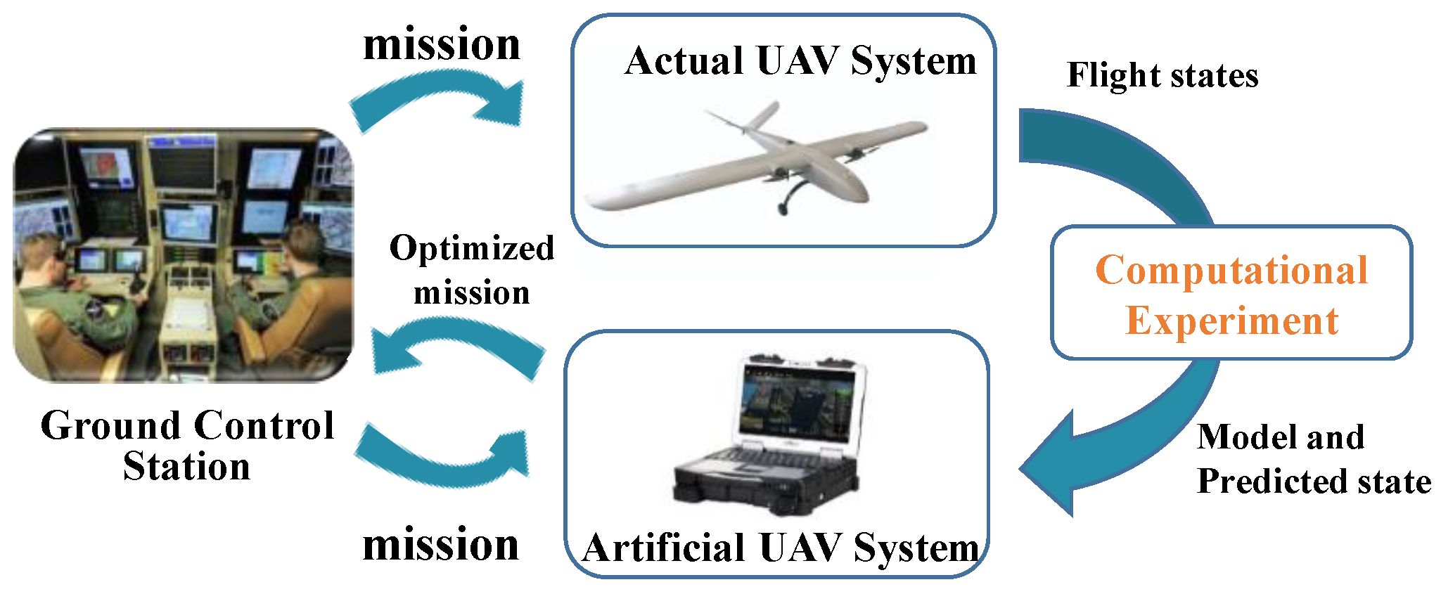
The basic framework of a parallel UAV system is established as shown in Figure 1. There is a one-to-one artificial UAV system corresponding to the aerial swarm UAV on the ground, while each artificial UAV system contains a baseline dynamics model of UAV and a controller model consistent with the airborne. The artificial UAV running on the time axis is several control cycles ahead of the real system. On the one hand, an iterative-optimized artificial system is developed by making continuous real-time corrections based on the real system operating status data returned by the data link to approach the actual system. Furthermore, the future trend and possible accidents of the actual system can be predicted by combining with the environmental data. The traditional control mode, in which the operator directly assigns tasks to the UAV swarm, is transformed into the parallel control mode, in which tasks are both assigned to the actual system and the parallel system at the same time. The parallel UAV system optimizes top-level tasks in real-time according to the predicted system status and uploads the optimized tasks to the ground control station. This can reduce the burden on the operator while ensuring the effectiveness of UAV control over the swarm, and improve the control capability of the UAV swarm.

The method in this paper uses a parallel UAV system as an auxiliary decision-making layer and decouples the control problem of UAV swarms, a complex time-varying system, with the support of huge computing resources on the ground. Moreover, the continuously revised parallel UAV model also guarantees the effectiveness of the control. The swarm control method proposed in this article is expected to greatly reduce the time, manpower and material costs, and find a new solution to the large-scale UAV swarm control problem.

2. Problem Statement

In order to realize the parallel control of the UAV swarm through a parallel UAV system, it is necessary to study the modeling method, state prediction method and real-time task replanning method, which can meet the requirements of parallel control accuracy. This paper mainly studies the modeling method and state prediction method of parallel UAV.

The key to realizing a parallel UAV system is to obtain a real-time and accurate parallel UAV model. The traditional accurate modeling method needs a wind tunnel experiment, which is expensive and complex. Therefore, a more practical, real-time and available modeling method with accuracy that satisfies parallel prediction and parallel control is needed. The system identification has the characteristics of simplicity, efficiency and low cost, so this paper uses the system identification method to model the parallel UAV.

System identification has three elements: identification data, model structure and identification criterion. The identification criterion is determined by the identification method. The identification data can be obtained by collecting flight data from the actual UAV system.

Hence, the identification data collected from the actual UAV system can be defined as

$$X=\left\{{\mathit{x}}_{i,m}=\left(x_{i,1},x_{i,2},\dots ,x_{i,M}\right),i\in \{1,2,\dots ,N\}\right\}$$

(1)

where ${\mathit{x}}_{i,m}$ denotes the multivariable observations at a particular time step, $x_{i,1},x_{i,2},\dots ,x_{i,M}$ is the value of the variable at time step $i$, and $M$ is the number of UAVs in the UAV swarm.

Then, the structure of the identification model needs to be determined. Common model structures are the state space model, the differential equation model and the transfer function model. The UAV system is a typical multiple-input multiple-output (MIMO) system, and the state-space model can well reflect the actual physical characteristics of the MIMO system. Therefore, the identification model can be defined as

$$\{\begin{array}{c}\mathit{x}(k+1)=A\mathit{x}(k)+B\mathit{u}(k)\\ \mathit{y}(k)=C\mathit{x}(k)+D\mathit{u}(k)+\mathit{n}(k)\end{array}$$

(2)

Among them, $\mathit{x}$ is the state vector of the system, $\mathit{y}$ is the output vector of the system, $\mathit{u}$ is the input vector of the system, $\mathit{n}$ is the noise vector, and $ABCD$ is the coefficient matrix of the system.

In order to improve the identification effect, the lateral and longitudinal identification models of UAV are established in this paper.

In the longitudinal drone model, there are

$$\{\begin{array}{c}\mathit{x}(k)={\left[\begin{array}{cccc}{V}_x(k)& V_z(k)& Q(k)& \theta (k)\end{array}\right]}^T\\ \mathit{u}(k)={\left[\begin{array}{cc}{\delta }_{elev}(k)& {\delta }_{thr}(k)\end{array}\right]}^T\\ D=0\end{array}$$

(3)

where $V_x$ is the speed along the x-axis in the airframe coordinate system, $V_z$ is the speed along the z-axis in the airframe coordinate system, $Q$ is the pitch angular velocity, $\theta$ is the pitch angle, ${\delta }_{elev}$ is the elevator deflection angle, and ${\delta }_{thr}$ is the throttle control amount.

In the lateral drone model, there are

$$\{\begin{array}{c}\mathit{x}(k)={\left[\begin{array}{ccccc}\varphi (k)& \psi (k)& P(k)& R(k)& V_y(k)\end{array}\right]}^T\\ \mathit{u}(k)={\left[\begin{array}{cc}{\delta }_{ail}(k)& {\delta }_{rud}(k)\end{array}\right]}^T\\ D=0\end{array}$$

(4)

where $\varphi$ is the roll angle, $\psi$ is the yaw angle, $P$ is the roll angular velocity, $R$ is the yaw angular velocity, $V_y$ is the speed along the y-axis in the airframe coordinate system, ${\delta }_{ail}$ is the aileron deflection angle, and ${\delta }_{rud}$ is the rudder deflection angle.

3. Approach

3.1. Model Identification

The subspace identification method is often used to identify the dynamic model of aircraft and can obtain a relatively good MIMO model without the initial model of the system. However, on the one hand, due to the lack of optimal process, the model identified by the subspace identification method is often sub-optimal. In order to obtain the optimal solution, the results need to be further optimized. On the other hand, when identifying high-order MIMO system models, the optimization-based identification algorithm is sensitive to the initial conditions, and generally, it is necessary to use the approximate optimal model as the initial conditions. Thus, in order to obtain better identification results, this paper proposes a two-step data-driven identification method: firstly, given the absence of the initial model of the system, the UAV dynamic model can be obtained directly from the identification data through the subspace identification method. Then, on the basis of the identification results in the first step, the prediction error identification method based on the optimization algorithm is used to further optimize the results for optimal solution.

Firstly, the subspace identification algorithm is used for identification. The subspace identification method integrates system theory, linear algebra and statistics, and can directly estimate the state-space model of the MIMO system from input–output data [21,22,23]. The basic idea is to obtain the model parameters from the row subspace and column subspace of the input–output Hankel matrix projection.

Suppose the discrete state space equation of the system is Equation (2).

Assuming that the noise $\mathit{n}$ is not related to the inputs $\mathit{u}$ and the above system is controllable and observable,

Make:

$$Y_q(k)=\left[\mathit{y}(k),\mathit{y}(k+1),\dots ,\mathit{y}(k+q-1)\right]$$

(5)

$U_q(k)$ and $N_q(k)$ are defined in the same way as $Y_q(k)$.

Then:

$$Y_q(k)=O_q\mathit{x}(k)+{\mathsf{\Gamma }}_q{U}_q(k)+N_q(k)$$

(6)

where:

$O_q$ is the extended observability matrix of the system:

$$O_q={(C CA \dots C{A}^{q-1})}^T$$

(7)

${\mathsf{\Gamma }}_q$ is the lower triangular Toeplitz matrix:

$${\mathsf{\Gamma }}_q=\left(\begin{array}{cccc}D& 0& \cdots & 0\\ CB& D& \cdots & 0\\ ⋮& ⋮& \ddots & ⋮\\ C{A}^{q-2}B& C{A}^{q-3}B& \cdots & D\end{array}\right)$$

(8)

Then make:

$$\begin{array}{l}Y=\left[Y_q(1)\hspace{1em}{Y}_q(2)\cdots Y_q(N)\right]\hfill \\ X=\left[\begin{array}{l}x(1)\hspace{1em}x(2)\hspace{1em}\cdots \hspace{1em}x(N)\hfill \end{array}\right]\hfill \\ U=\left[\begin{array}{llll}{U}_q(1)\hfill & U_q(2)\hfill & \cdots \hfill & U_q(N)\hfill \end{array}\right]\hfill \\ N=\left[\begin{array}{llll}{N}_q(1)\hfill & N_q(2)\hfill & \cdots \hfill & N_q(N)\hfill \end{array}\right]\hfill \end{array}$$

(9)

One can then get:

$$Y=O_{q}X+{\mathsf{\Gamma }}_{q}U+N$$

(10)

Then, the orthogonal basis of $U$ can be defined as:

$${\mathsf{\Pi }}_{U^H}^{\perp }=I-U^H{(U{U}^H)}^{-1}U$$

(11)

Multiply both sides of Equation (10) by ${\mathsf{\Pi }}_{U^H}^{\perp }$ to get:

$$Y{\mathsf{\Pi }}_{U^H}^{\perp }=O_{q}X{\mathsf{\Pi }}_{U^H}^{\perp }+N{\mathsf{\Pi }}_{U^H}^{\perp }$$

(12)

Singular value decomposition of $Y{\mathsf{\Pi }}_{U^H}^{\perp }$:

$$\left(\mathrm{Re}\left(Y{\mathsf{\Pi }}_{U^H}^{\perp }\right)\hspace{1em}\mathrm{Im}\left(Y{\mathsf{\Pi }}_{U^H}^{\perp }\right)\right)=\left(\begin{array}{ll}{U}_s\hfill & U_0\hfill \end{array}\right)\left(\begin{array}{cc}{\mathsf{\Sigma }}_s& 0\\ 0& {\mathsf{\Sigma }}_0\end{array}\right)\left(\begin{array}{l}{V}_s^T\hfill \\ V_0^T\hfill \end{array}\right)$$

(13)

where $U_s$ is the singular value vector, ${\mathsf{\Sigma }}_s$ is the corresponding singular value.

The column space of $Y{\mathsf{\Pi }}_{U^H}^{\perp }$ and $O_q$ is the same [23]. Thus, $Y{\mathsf{\Pi }}_{U^H}^{\perp }$ and $O_q$ have the same singular value. Therefore, the estimate of $O_q$ can be calculated by

$${\widehat{O}}_q=U_s{{\mathsf{\Sigma }}_s}^{1/2}$$

(14)

Then, combining Equations (7) and (14) can directly obtain the estimated value $\widehat{A},\widehat{C}$ of $A,C$.

According to the following formula, the estimated value $\widehat{B},\widehat{D}$ of $B,D$ can be obtained by solving the least square problem:

$$\arg \underset{B,D\in R}{\min }{\displaystyle \sum _{k=1}^N{\Vert \mathit{y}(t)-\widehat{C}{(qI-\widehat{A})}^{-1}B\mathit{u}(t)-D\mathit{u}(t)-\widehat{C}{(qI-\widehat{A})}^{-1}{\mathit{x}}_0\delta (t)\Vert }^2}$$

(15)

where $I$ is the Identity matrix, ${\mathit{x}}_0$ is the initial state, and $\delta (t)$ is unit pulse input at time 0.

Then, the identification result of the subspace identification algorithm will be obtained, which will be used as the initial model of the prediction error method.

Define error vector:

$$\mathit{\epsilon }=Y-\widehat{Y}$$

(16)

Among them, $Y$ is the actual measured value, and $\hat{Y}$ is the model’s estimated value.

The objective function is defined as

$$J={\mathit{\epsilon }}^T\mathit{\epsilon }$$

(17)

In order to obtain the best fitting model with the experimental data, the objective function $J$ should be minimized. The estimation parameters can be obtained by the Newton–Raphson method [24] and the identification model can be obtained.

3.2. Data Processing

3.2.1. Data Preprocessing

Since the actual data communication process may cause data packet loss and communication delay, in order to make the collected data reflect the flight status of the UAV as truly as possible, the collected flight data must be preprocessed (including time-stamp calibration and interpolation correction).

The data collected from the actual system contain time information. Therefore, taking the pitch angle data $\theta$ as an example, it can be defined as:

$${\mathit{x}}_{i,\theta }=[dat{a}_{\theta }(i),tim{e}_{\theta }(i)],(i=0,1,2,\cdots ,N)$$

(18)

where $dat{a}_{\theta }(i)$ is the specific value of pitch angle and $tim{e}_{\theta }(i)$ is the data collection time.

Firstly, time calibration is performed on these data. Then, the Lagrange interpolation method is used to complete the data lost during transmission.

For example:

For the known n + 1 sampling points $(a_0,b_0)\dots (a_{n+1},b_{n+1})$, the Lagrange interpolation formula is:

$$\begin{array}{l}L(a)={\displaystyle \sum _{i=0}^n{b}_i{l}_i(a)}\\ l_i(a)={\displaystyle \prod _{j=0,j\ne i}^n\frac{a-a_j}{a_i-a_j}},(i=0,1,2,\cdots ,n)\end{array}$$

(19)

Part of the data lost during the transmission process can be supplemented by Formula (20), so as to solve the problem of data packet loss and time delay during the data transmission process.

3.2.2. Sliding Time Window Method

A critical problem that usually exists in online identification is “data saturation”, which indicates that the ever-growing data collected during experiments may be overwhelmed by old data [25]. This may cause the parameter estimates to fail to track changes in time-varying parameters, resulting in a gradual loss of correction ability of the algorithm. This is because, if the identification algorithm gives the same reliability to both new and old data, then the amount of information obtained from the new data decreases accordingly.

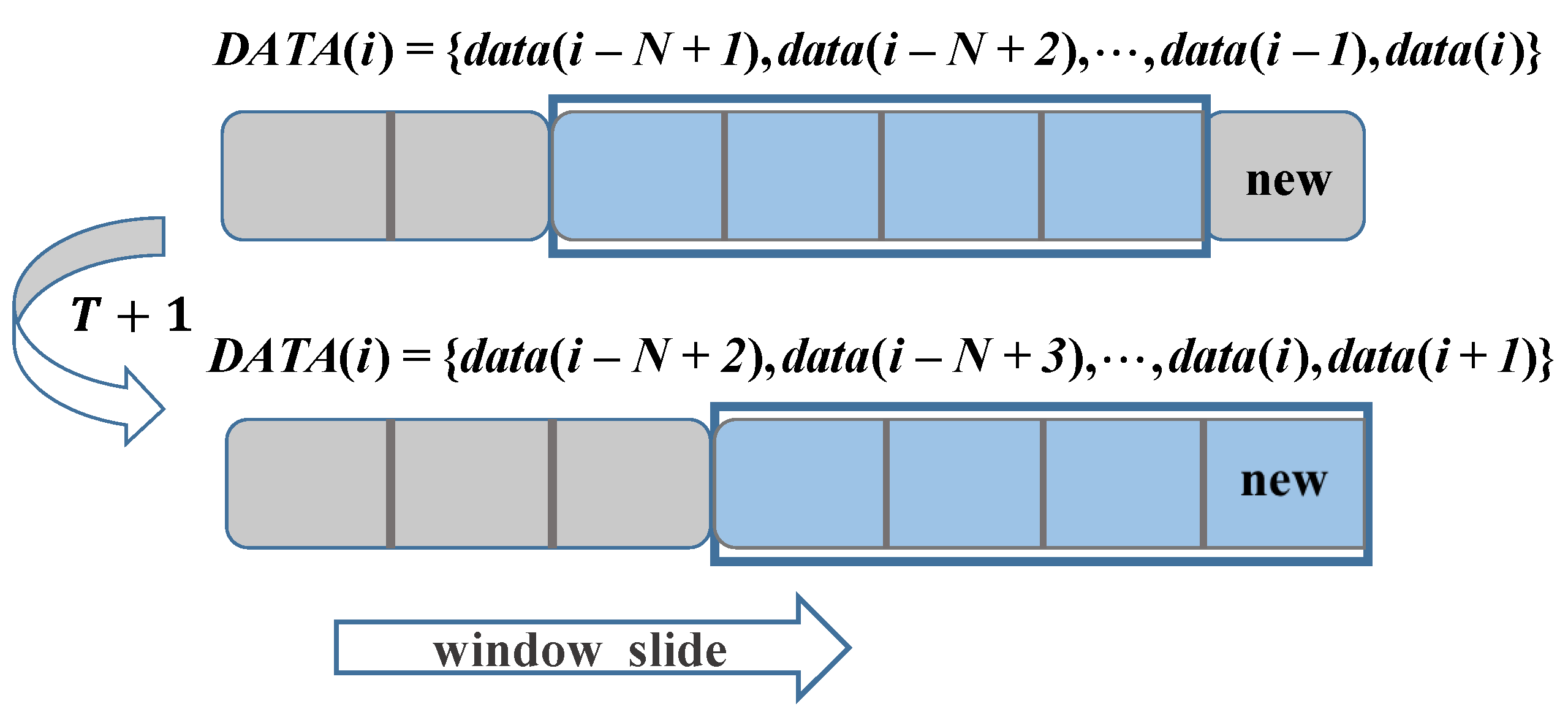
To solve this, the sliding time window [26] method is developed. The sliding time window method only identifies the latest N data each time, and all the previous data are abandoned, as shown in Figure 2.

For example, when $T=i$, the identification data are:

$$DATA(i)=\{data(i-N+1),data(i-N+2),\cdots ,data(i-1),data(i)\}$$

(20)

Then, when $T=i+1$, a new data point $data(i+1)$ is added and an old data $data(i-N+1)$ point is eliminated:

$$DATA(i+1)=\{data(i-N+2),data(i-N+3),\cdots ,data(i),data(i+1)\}$$

(21)

In this way, it is maintained that only the latest N data are taken for calculation each time, thereby ensuring that the information provided by the new data will not be overwhelmed by the old data, so the algorithm can always correct the model.

3.3. Model Verification

To guarantee that the artificial UAV system is always up to date corresponding to the physical UAV system, it is necessary to perform model verification on the identification results. The validation of the identification model was performed by comparing the model response with the real flight data.

In previous literature, various model quality metrics have been put forward to evaluate the quality of the identified model. The normalized root mean square error (NRMSE) is often used to measure the deviation between the estimated value and the actual value. Thus, this paper uses NRMSE as the fit metric of the model response and the flight data to judge the quality of the identification model. The calculation formula of NRMSE fitness value is:

$$fit=(1-\frac{\Vert \mathit{y}-\widehat{\mathit{y}}\Vert }{\Vert \mathit{y}-\overline{\mathit{y}}\Vert })\times 100\%$$

(22)

where $\mathit{y}$ is the actual flight data, $\widehat{\mathit{y}}$ is the model estimation data, and $\overline{\mathit{y}}$ is the mean value of $\mathit{y}$. $fit$ varies between $-\infty$ (bad fit) and 100 (perfect fit). When the $fit$ is greater than 0, the model fits the data better than the sample mean of the output, so the identification result is acceptable.

3.4. State Prediction

The UAV system is a typical causal system, whose outputs are only related to the current states and inputs. When the system is at the moment k, ignoring the output noise, its state outputs can be defined as:

$$\{\begin{array}{c}\mathit{y}(k)=C\mathit{x}(k)+D\mathit{u}(k)\\ \mathit{x}(k+1)=A\mathit{x}(k)+B\mathit{u}(k)\end{array}$$

(23)

Then, the predicted output is:

$$\widehat{\mathit{y}}(k+n)=C\widehat{\mathit{x}}(k+n)+D\widehat{\mathit{u}}(k+n)$$

(24)

where:

$$\begin{array}{l}\widehat{\mathit{x}}(k+n)=A\hat{\mathit{x}}(k+n-1)+B\hat{\mathit{u}}(k+n-1)\\ \widehat{\mathit{x}}(k+n-1)=A\hat{\mathit{x}}(k+n-2)+B\widehat{\mathit{u}}(k+n-2)\\ ⋮\\ \widehat{\mathit{x}}(k+1)=A\mathit{x}(k)+B\mathit{u}(k)\end{array}$$

(25)

which is:

$$\hat{\mathit{x}}(k+n)=A^n\mathit{x}(k)+A^{n-1}B\mathit{u}(k)+A^{n-2}B\hat{\mathit{u}}(k+1)+\cdots +AB\hat{\mathit{u}}(k+n-2)+B\hat{\mathit{u}}(k+n-1)$$

(26)

where $\hat{\mathit{x}}(•)$ is the prediction value of states, $\widehat{\mathit{u}}(•)$ is the prediction value of inputs. $\mathit{x}(k)$ and $\mathit{u}(k)$ are the actual system states and inputs at moment k.

Then, to obtain the predicted outputs value, the predicted inputs value needs to be obtained. For the UAV system in this article, the inputs are the control amount of the rudder surface and the throttle, which are calculated by the flight controller according to the status and route of the UAV. Therefore, by simply sending the state prediction value $\widehat{\mathit{x}}(k+n-1)$ to the controller, the inputs $\widehat{\mathit{u}}(k+n)$ are obtained.

This article uses two identical flight controllers as the flight controllers for the actual UAV system and the artificial UAV system, which loads them with the same mission route. The state prediction process is shown in Figure 3:

First, by using the system inputs $\mathit{u}(k)$ and the states $\mathit{x}(k)$, the predicted states $\widehat{\mathit{x}}(k+1)$ and the predicted outputs $\widehat{\mathit{y}}(k)$ are calculated according to Formula (24). Then, the predicted states $\widehat{\mathit{x}}(k+1)$ of the UAV system are sent to the flight controller, and the control information returned by the flight controller is used as the predicted inputs $\widehat{\mathit{u}}(k+1)$. The process above is cyclic; thus, the predicted states of the system can be obtained by repeating the process.

3.5. Method Overview

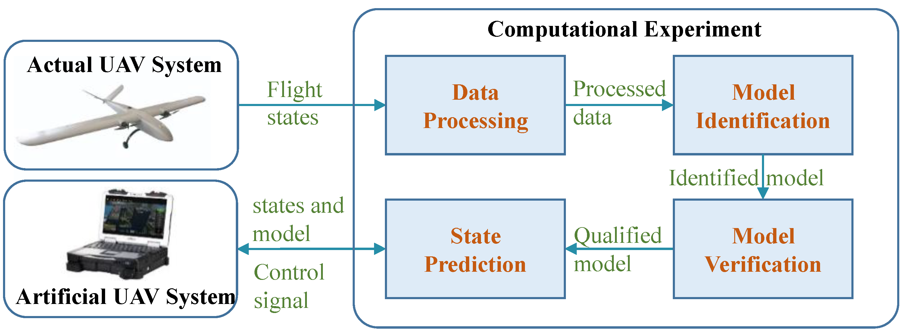
The method overview of this article is as follows: through Computational Experiment, after processing the flight states data of the actual UAV system, the model identification method is used to identify the system model, and the result is used as the model of the artificial system after the model is verified to be qualified, and the modeling of the artificial UAV system is realized. Finally, the predicted states of the actual UAV system can be obtained through the state prediction method of the artificial UAV system, as Figure 4 shows.

Algorithm 1 outlines the Computational Experiments Algorithm of this article. Flight data are obtained by real-time sampling. Data_preprocess() and Time_window_sliding() are used to process flight data. Firststep_Identify() and Refine_Identify() are used to identify the system model. Moreover, Model_verify() is used to perform model verification on the identification results. State_prediction() is used to predict the states of UAV system. In order to improve the accuracy of system identification, it is necessary to preprocess the flight data. To solve the data saturation problem, the sliding time window method is used to process flight data. Then, a two-step data-driven identification method is applied to identify model parameters. Finally, model verification is performed and the threshold $\varpi$ is set. The data fitting value is calculated. If Fit_value is greater than $\varpi$, the qualified model is used for state prediction. Otherwise, model identification is performed again.

Algorithm 1 Computational Experiments Algorithm
Input: -Flight_data: the real-time flight states -Model_input: the control signal
Output: -Qualified_model: the qualified identification model -Predicted_data: the predicted states
Workflow(Repeat):
1:	Preprocessed_data = Data_preprocess (Flight_data);
2:	Identify_data = Time_window_ sliding (Preprocessed_data);
3:	Firststep_model = Firststep_Identify (Identify_data);
4:	Refined_model = Refine_Identify (Identify_data, Firststep _model);
5:	Fit_value = Model_verify (Refined_model, Flight_data);
6:	if Fit_value < $\varpi$
7:	goto 3
8:	else
9:	Qualified_model = Refined_model;
10:	end if
11:	Predicted_state = State_prediction(Qualified_model, Model_input);
12:	return Qualified_model and Predicted_state

4. Results and Discussion

4.1. Experimental Setup

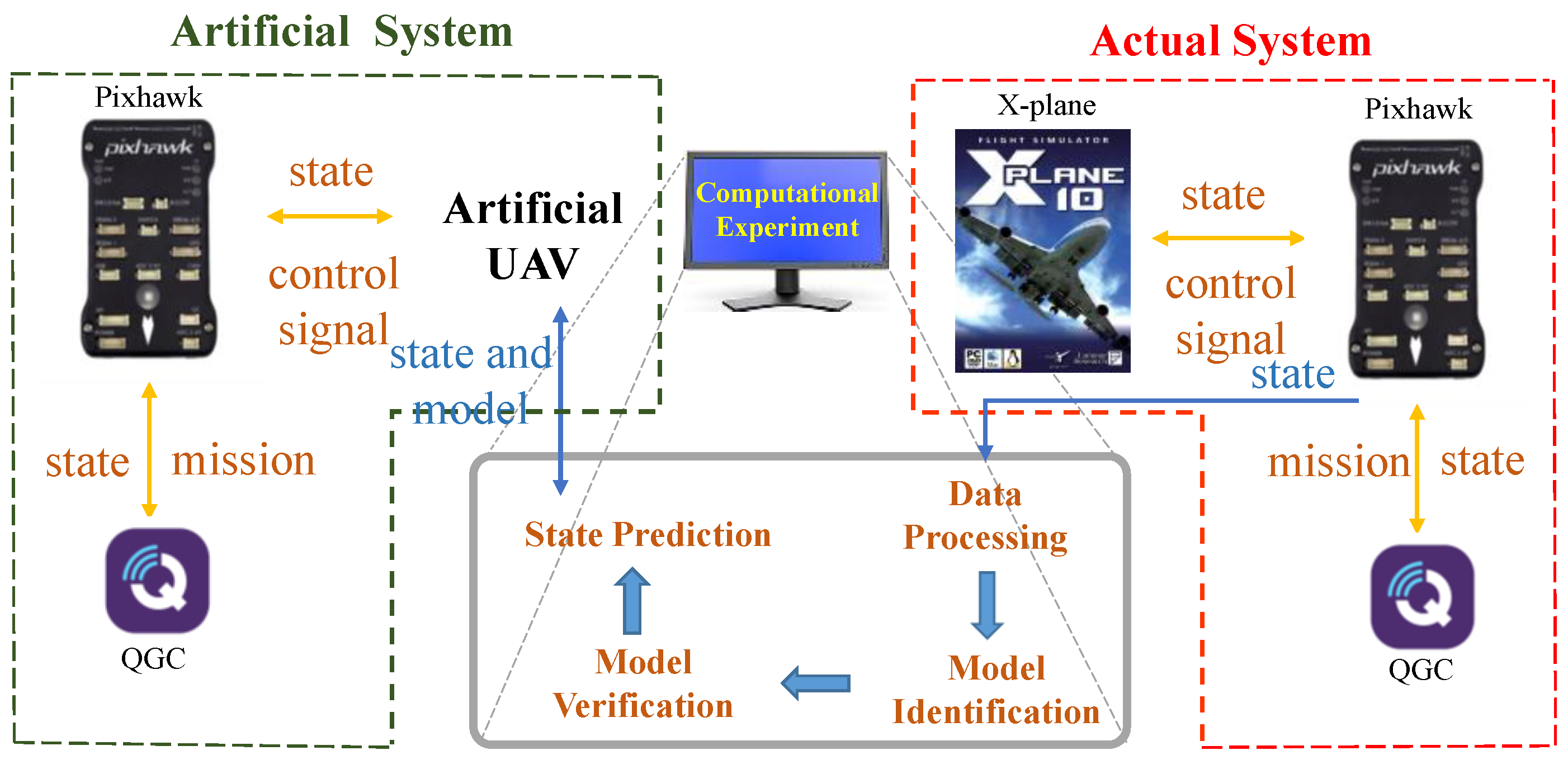
To verify the feasibility and effectiveness of our proposed method, we build a UAV hardware-in-the-loop (HITL) real-time simulation system [27] and conduct the flight simulation experiments based on this system.

As shown in Figure 5, the established HITL simulation system is composed of an X-Plane flight simulation software, a qgroundcontrol (QGC) ground control station, and two pixhawks flight controllers. X-plane is a professional flight simulation software with highly realistic airplane models. Pixhawk is a common UAV flight controller, widely used in flight control of fixed-wing UAV and rotary-wing UAV. QGC is a UAV ground control station software. The UAV HITL real-time simulation system based on X-Plane, pixhawk and QGC works well on simulating a real UAV flight and is free of environmental conditions when conducting flight test and data collection.

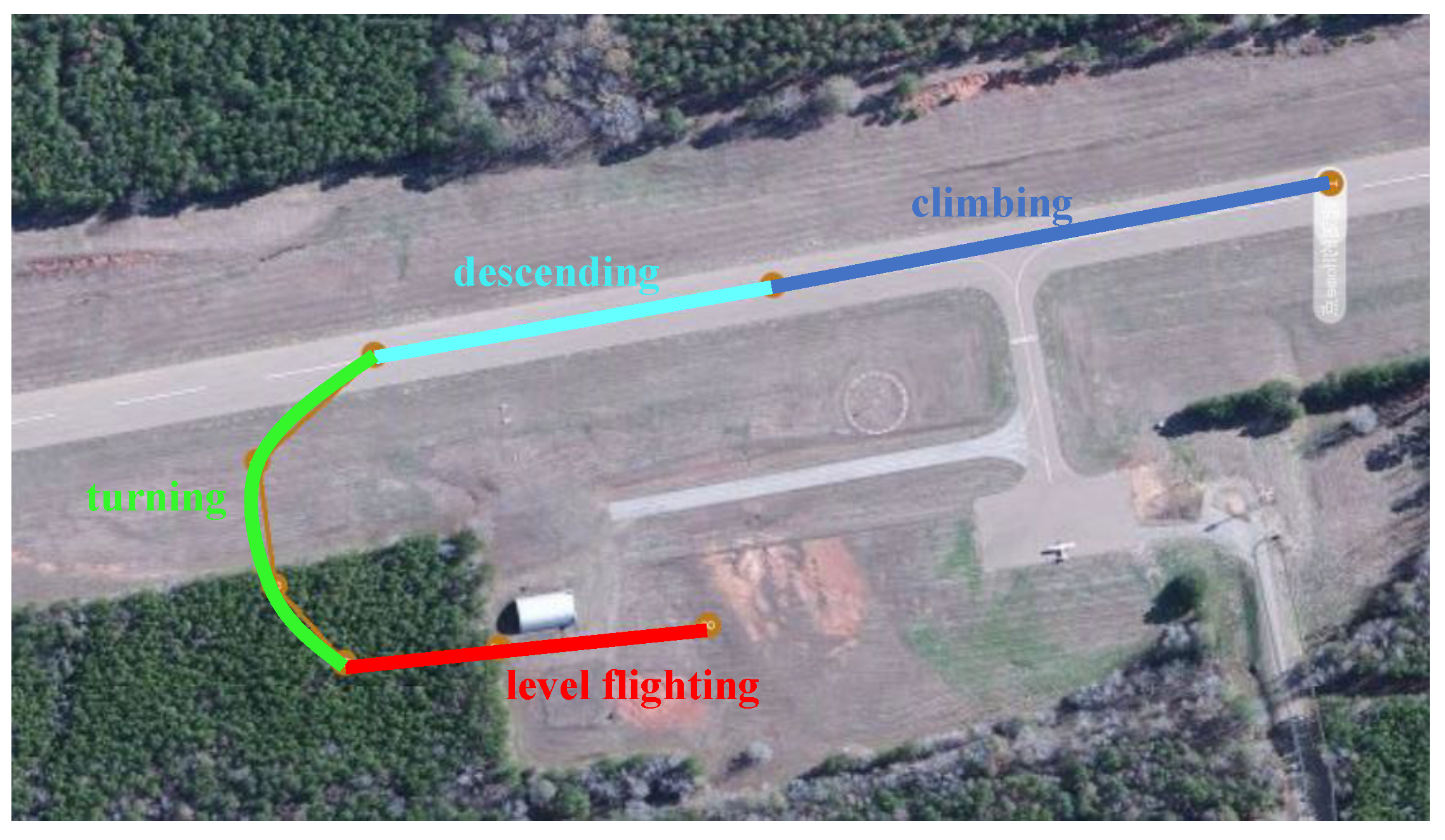
There are many modes in UAV mission flight. In this paper, the four most common modes (including climbing, descending, turning and level flighting) are selected for experiments. Therefore, this paper designs a mission flight route that includes all four modes (as shown in Figure 6).

4.2. Model Identification Experiment

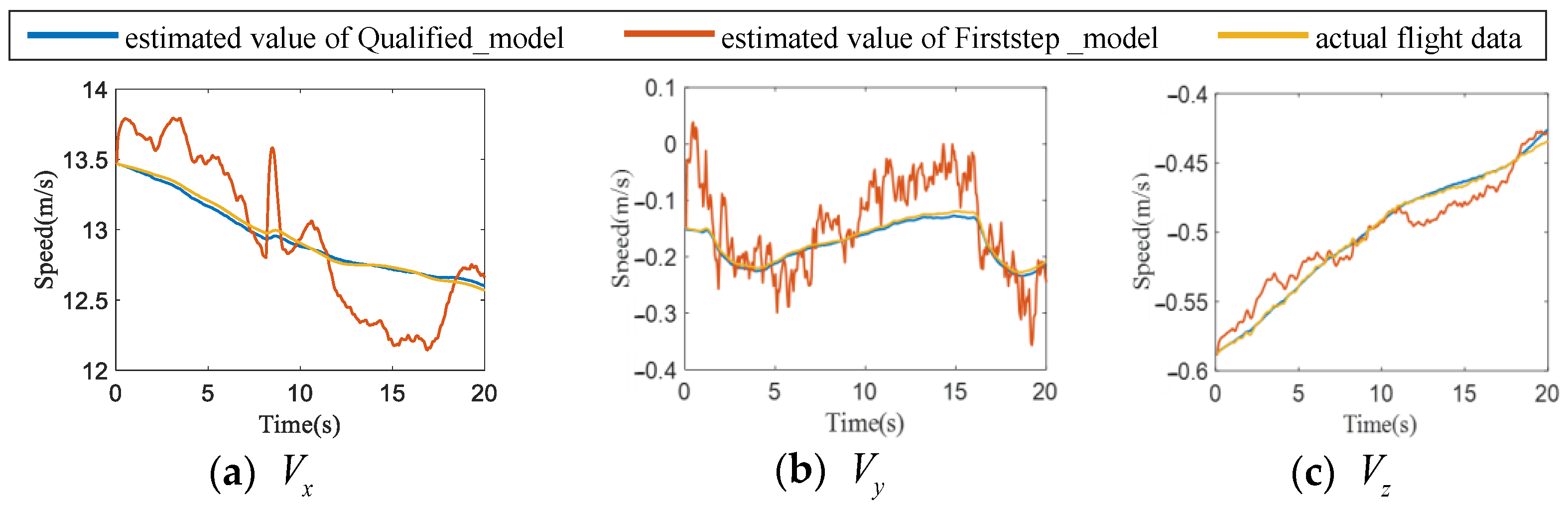
In this paper, a subspace identification method and a two-step data-driven identification method are used to identify the dynamic model of UAV in flight. Take the UAV speed as an example: Figure 7 shows the comparison between the actual data and the model estimation of the two identification results. The yellow line refers to the actual flight data corresponding to state, the red line indicates the estimated value of the Firststep_model, and the blue line shows the estimated value of the Qualified_model. It can be seen intuitively that the model estimation of the Qualified_model is closer to the real data than the estimation of the Firststep_model. This shows that the identification model obtained by the two-step data-driven identification method can reflect the physical characteristics of the actual model better than the identification model obtained by the subspace method. This proves the effectiveness of the two-step data-driven identification method.

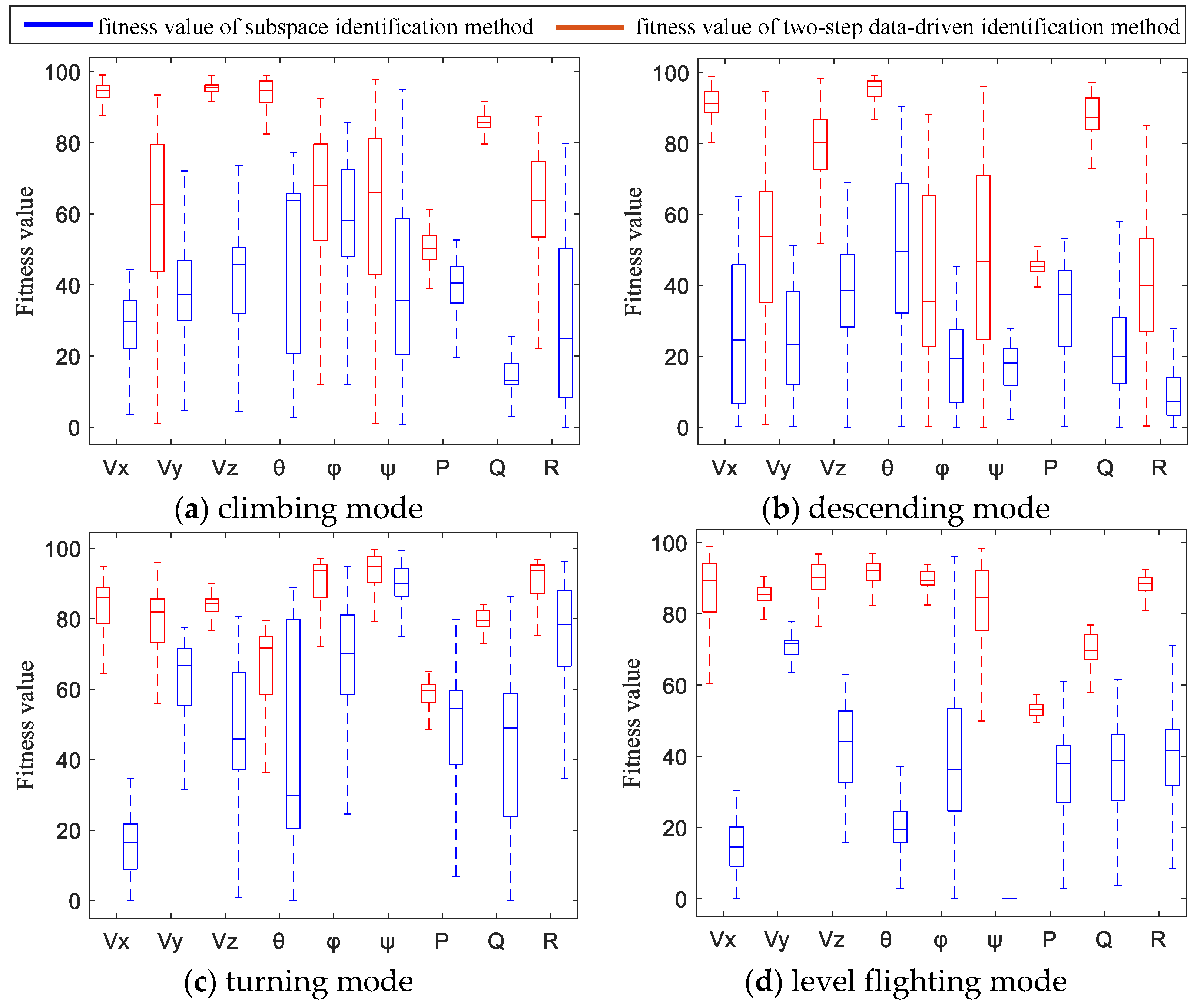
A quantitative analysis of the two identification results is given below: 100 identification experiments were carried out in four flight modes, and the results were statistically analyzed. Figure 8 shows the box diagram of both the NRMSE fitness value of each state of subspace identification method and the two-step data-driven identification method proposed in this paper. Among them, the red diamond refers to the result of the two-step data-driven identification method, and the blue diamond is the result of the subspace identification method. It can be seen that the fit value of the two-step data-driven identification method is significantly greater than the fit value of the subspace identification method, indicating that the two-step data-driven identification method can better identify the actual model than the subspace identification method.

4.3. State Prediction Experiment

According to the state prediction method proposed in this paper, the identification model based on the two-step data-driven identification method is used to predict the flight states of the UAV.

Figure 9a shows the comparison of mission route, actual trajectory and predicted trajectory for 60 s from a certain moment. The blue line is the given mission route, the red line is the actual flight trajectory and the yellow line is the predicted flight trajectory. Figure 9b shows the relative error between the predicted value and the actual value of the spatial location. Then, this paper conducted 20 prediction experiments and counted the times when the relative error was less than 10%. Figure 9c shows the boxplot of the time when the relative error is less than 10% in 20 prediction experiments. When the relative error is less than 10%, it can be seen that the time fluctuates around 20 s. Taking the lower quartile of the above statistical results of 16.5 s as the prediction confidence value, this paper considers that the parallel system and state prediction method proposed can basically guarantee that the prediction states error is kept within 10% for about 16 s. If there is a communication interruption, the predicted state of the parallel UAV system can be maintained at about 10% within the first 16 s of the communication interruption. Then, according to the parallel control method, the parallel UAV system can use these predicted states to find out unexpected situations that may occur, and promptly generate dangerous disposal plans, which improves the efficiency of emergency handling of dangerous events and thus improves the effectiveness of cluster control.

5. Conclusions and Future Work

In order to solve the problem of how to improve the effectiveness of UAV swarm control in non-ideal environments, this paper proposes a parallel swarm control method and studies the model identification and state prediction methods. The experimental results of model estimation and state prediction show that the model outputs obtained by the identification method have a good consistency with the actual flight data, and the state prediction error can be kept below 10% about 16 s, indicating that the effectiveness of swarm control can be guaranteed within 16 s of communication interruption.

In the future, the real-time task replanning method will be further studied based on the parallel artificial UAV system. Combined with the existing research results, the parallel UAV system is improved to provide a new solution for UAV swarm control.

References

- Wang, F.Y. Parallel Control and Management for Intelligent Transportation Systems: Concepts, Architectures, and Applications. IEEE Trans. Intell. Transp. Syst. 2010, 11, 630–638. [Google Scholar] [CrossRef]
- Wang, F.Y. Computational Experiments for Behavior Analysis and Decision Evaluation of Complex Systems. J. Syst. Simul. 2004, 16, 893–897. [Google Scholar]
- Jin, J.; Guo, H.; Xu, J. An End-to-End Recommendation System for Urban Traffic Controls and Management under a Parallel Learning Framework. IEEE Trans. Intell. Transp. Syst. 2020, 22, 1616–1626. [Google Scholar] [CrossRef]
- Zhang, H.; Luo, G.; Tian, Y. A Virtual-Real Interaction Approach to Object Instance Segmentation in Traffic Scenes. IEEE Trans. Intell. Transp. Syst. 2020, 22, 863–875. [Google Scholar] [CrossRef]
- Zhu, F.; Lv, Y.; Chen, Y. Parallel Transportation Systems: Toward IoT-Enabled Smart Urban Traffic Control and Management. IEEE Trans. Intell. Transp. Syst. 2019, 21, 4063–4071. [Google Scholar] [CrossRef]
- Li, L.; Wang, X.; Wang, K. Parallel testing of vehicle intelligence via virtual-real interaction. Science 2019, 4, eaaw4106. [Google Scholar] [CrossRef]
- Wang, F.Y. Parallel Driving with Software Vehicular Robots for Safety and Smartness. IEEE Trans. Intell. Transp. Syst. 2014, 15, 1381–1387. [Google Scholar] [CrossRef]
- Wang, F.Y.; Zheng, N.N.; Cao, D.P. Parallel Driving in CPSS: A Unified Approach for Transport Automation and Vehicle Intelligence. IEEE/CAA J. Autom. Sin. 2017, 4, 577–587. [Google Scholar] [CrossRef] [Green Version]
- Wang, X.; Li, L.X.; Yuan, Y. ACP Based Social Computing and Parallel Intelligence: Societies 5. 0 and Beyond. CAAI Trans. Intell. Technol. 2016, 1, 377–393. [Google Scholar] [CrossRef]
- Wang, X.; Zheng, X.H.; Zhang, X.Z. Analysis of Cyber Interactive Behaviors Using Artificial Community and Computational Experiments. IEEE Trans. Syst. Man Cybern. 2017, 47, 995–1006. [Google Scholar] [CrossRef]
- Yuan, Y.; Wang, F.Y.; Zeng, D.L. Developing a Cooperative Bidding Framework for Sponsored Search Markets-An Evolutionary Perspective. Inf. Sci. 2016, 369, 674–689. [Google Scholar] [CrossRef]
- Qin, R.; Yuan, Y.; Wang, F.Y. Exploring the Optimal Granularity for Market Segmentation in RTB Advertising via Computational Experiment Approach. Electron. Commer. Res. Appl. 2017, 24, 68–83. [Google Scholar] [CrossRef]
- Yuan, Y.; Zeng, D.D. Co-evolution Based Mechanism Design for Sponsored Search Advertising. Electron. Commer. Res. Appl. 2012, 11, 537–547. [Google Scholar] [CrossRef]
- Wang, F.Y. Toward a Paradigm Shift in Social Computing: The ACP Approach. IEEE Intell. Syst. 2007, 22, 65–67. [Google Scholar] [CrossRef]
- Wang, F.Y.; Wang, X.; Li, L.X. Steps toward Parallel Intelligence. IEEE/CAA J. Autom. Sin. 2016, 3, 345–348. [Google Scholar]
- Wang, F.Y.; Zhang, J.J.; Zheng, X.H. Where Does AlphaGo Go: From Church Turing Thesis to AlphaGo Thesis and Beyond. IEEE/CAA J. Autom. Sin. 2016, 3, 113–120. [Google Scholar]
- Wang, F.Y.; Yang, L.Q.; Cheng, X. Network Softwarization and Parallel Networks: Beyond Software Defined Networks. IEEE Netw. 2016, 30, 60–65. [Google Scholar] [CrossRef]
- Wang, F.Y.; Zhang, J.; Wei, Q.L. PDP: Parallel Dynamic Programming. IEEE/CAA J. Autom. Sin. 2017, 4, 1–5. [Google Scholar] [CrossRef]
- Wang, K.F.; Gou, C.; Zheng, N.N. Parallel Vision for Perception and Understanding of Complex Scenes: Methods, Framework, and Perspectives. Artif. Intell. Rev. 2017, 48, 298–328. [Google Scholar] [CrossRef]
- Kang, M.Z.; Wang, F.Y. From Parallel Plants to Smart Plants: Intelligent Control and Management for Plant Growth. IEEE/CAA J. Autom. Sin. 2017, 4, 161–166. [Google Scholar] [CrossRef]
- Overschee, P.V.; Moor, B.D. Subspace Algorithms for the Stochastic Identification Problem. Automatica 1993, 29, 649–660. [Google Scholar] [CrossRef]
- Verhaegen, M. Identification of the Deterministic Part of MIMO State Space Models Given in Innovations Form From Input Output Data. Automatica 1994, 30, 61–74. [Google Scholar] [CrossRef]
- Overschee, P.V.; Moor, B.D. N4SID: Subspace Algorithms for the Identification of Combined Deterministic-Stochastic Systems. Automatica 1994, 30, 75–93. [Google Scholar] [CrossRef]
- Ding, F.; Liu, X.P.; Liu, G. Identification methods for Hammerstein nonlinear systems. Digit. Signal. Process. 2011, 21, 215–238. [Google Scholar] [CrossRef]
- Huang, Y.; Xiang, X.; Zhou, H. Refinement of UAV dynamics model through online identification: A model-data hybrid approach. In Proceedings of the 2020 Chinese Automation Congress (CAC), Shanghai, China, 6–8 November 2020. [Google Scholar]
- Wang, L.; Zhang, Y.; Cai, Y.P. Operational Mode Identification Based on Sliding Time Window Method and Eigensystem Realization Algorithm. Trans. Nanjing Univ. Aeronaut. Astronaut. 2019, 36, 838–844. [Google Scholar]
- Yan, C.; Xiang, X.; Wang, C. Fixed-Wing UAVs flocking in continuous spaces: A deep reinforcement learning approach. Robot. Auton. Syst. 2020, 131, 103594. [Google Scholar] [CrossRef]
Figure 1.
Basic framework of a parallel Unmanned Aerial Vehicle (UAV) system.
Figure 2.
The schematic diagram of sliding time window method.
Figure 3.
The state prediction process.
Figure 4.
The method overview of the parallel UAV system.
Figure 5.
UAV hardware-in-the-loop real-time simulation system.
Figure 6.
The mission flight route in our experiment.
Figure 7.
Comparison of flight data and model estimation data.
Figure 8.
Figure 9.
Display of predicted results. (a) is the comparison of mission route, actual trajectory and predicted trajectory. (b) is the relative error between the predicted value and the actual value of the spatial location. (c) is the box chart of the time when the relative error is less than 10% in 20 prediction experiments.
Publisher’s Note: MDPI stays neutral with regard to jurisdictional claims in published maps and institutional affiliations. |
© 2021 by the authors. Licensee MDPI, Basel, Switzerland. This article is an open access article distributed under the terms and conditions of the Creative Commons Attribution (CC BY) license (https://creativecommons.org/licenses/by/4.0/).
Share and Cite
MDPI and ACS Style
Huang, Y.; Xiang, X.; Zhou, H.; Tang, D.; Sun, Y. Online Identification-Verification-Prediction Method for Parallel System Control of UAVs. Aerospace 2021, 8, 99. https://doi.org/10.3390/aerospace8040099
AMA Style
Huang Y, Xiang X, Zhou H, Tang D, Sun Y. Online Identification-Verification-Prediction Method for Parallel System Control of UAVs. Aerospace. 2021; 8(4):99. https://doi.org/10.3390/aerospace8040099
Chicago/Turabian StyleHuang, Yixin, Xiaojia Xiang, Han Zhou, Dengqing Tang, and Yihao Sun. 2021. "Online Identification-Verification-Prediction Method for Parallel System Control of UAVs" Aerospace 8, no. 4: 99. https://doi.org/10.3390/aerospace8040099
Note that from the first issue of 2016, this journal uses article numbers instead of page numbers. See further details here.