Effect of Levels of Fidelity on Steady Aerodynamic and Static Aeroelastic Computations

Abstract

Static aeroelastic deformations are nowadays considered as early as in the preliminary aircraft design stage, where low-fidelity linear aerodynamic modeling is favored because of its low computational cost. However, transonic flows are essentially nonlinear. The present work aims at assessing the impact of the aerodynamic level of fidelity used in preliminary aircraft design. Several fluid models ranging from the linear potential to the Navier–Stokes formulations were used to solve transonic flows for steady rigid aerodynamic and static aeroelastic computations on two benchmark wings: the Onera M6 and a generic airliner wing. The lift and moment loading distributions, as well as the bending and twisting deformations predicted by the different models, were examined, along with the computational costs of the various solutions. The results illustrate that a nonlinear method is required to reliably perform steady aerodynamic computations on rigid wings. For such computations, the best tradeoff between accuracy and computational cost is achieved by the full potential formulation. On the other hand, static aeroelastic computations are usually performed on optimized wings for which transonic effects are weak. In such cases, linear potential methods were found to yield sufficiently reliable results. If the linear method of choice is the doublet lattice approach, it must be corrected using a nonlinear solution.

1. Introduction

In recent years, constraints on limiting air pollution generated by aircraft increased dramatically. For example, the European project Flightpath 2050 [1] aims at a reduction of 90% and 75% in $N{O}_x$ and $C{O}_2$ gas emissions, respectively. On the other hand, the aircraft market is becoming more and more competitive, so that aircraft having low operational cost are valued. As a consequence, extensive research is being carried out to reduce aircraft fuel consumption. Current design philosophies aim at reducing aircraft structural weight while maximizing aerodynamic efficiency. This approach often leads to the design of very flexible and highly loaded composite wings, with increased aspect ratio and complex shape. For such wings, aeroelastic deformations cannot be ignored as they can have a significant effect on the flight shape, hence the aerodynamic loading and efficiency of the wing. Aeroelasticity must therefore be integrated early in the aircraft design, typically in the preliminary stage, during which aero-structural design and optimization are performed. Since many design parameters and configurations are considered at this early stage, engineers usually select low-fidelity modeling to obtain results quickly. However, low fidelity aerodynamic models are linear, whereas most transport aircraft fly in the transonic regime, in which the flow is nonlinear. The objective of the present work is to assess the impact of the aerodynamic level of fidelity on steady aerodynamic and static aeroelastic computations typically performed in preliminary aircraft design.

Various comparison analyses have already been performed on rigid geometries. For example, Bhateley and Cox [2], Verhoff and O’Neil [3], and Rubbert and Saaris [4] used transonic small disturbances and linear potential theory to compute transonic flows over fighter configurations, and compared their results to nonlinear potential modeling or experimental data. In particular, Verhoff and O’Neil already suggested to resort to multi-fidelity modeling to extend transonic prediction capabilities by combining panel methods to nonlinear potential solvers. Flores et al. [5] compared full potential to Euler solvers using two-dimensional airfoils and showed that the nonlinear potential formulation was noticeably faster than the Euler formulation, for a similar accuracy in the integrated aerodynamic coefficients, as long as the shocks were weak. Klopfer and Nixon [6] further showed that adding a non-isentropic correction to the full potential formulation greatly improved the results for strong shocks. Several authors, such as Le Balleur [7], Melnik et al. [8], and Van Muijden et al. [9], also added an interactive boundary layer modeling capability to full potential solvers and were able to match experimental data. Validation of various full potential codes with respect to higher-fidelity data can be found in the survey work by Holst [10]. Drela et al. [11] , Potsdam [12], and Aftosmis et al. [13] also extended various Euler solvers with viscous-inviscid calculations. The latter compared their results to both Reynolds-Averaged Navier–Stokes computations and experimental data. Some authors also performed surveys to assess the capabilities and limitations of the different aforementioned aerodynamic levels of fidelity. For example, Jameson [14], and more recently Johnson et al. [15], regrouped and analyzed the comparison studies performed by various authors using different solvers. However, the computations are based on different geometries and are scattered across different years, which makes direct comparison difficult. Moreover, the emphasis is usually placed on model or methodology validation rather than on the tradeoff between accuracy and computational time. To the knowledge of the present authors, there still exists no systematic and extensive comparative studies of all major aerodynamic modeling methods for transonic flow on the same benchmarks.

Although engineers commonly use multi-fidelity [16] or high-fidelity [17,18] aerodynamic modeling, even fewer comparative studies are available for static aeroelasticity computations. The most extensive one is probably the first Aeroelastic Prediction Workshop organized by the American Institute of Aeronautics and Astronautics in 2012 [19,20]. In this workshop, some authors, such as Romanelli et al. [21] and Acar and Nikbay [22], compared their results obtained with linear potential or Euler equations to experimental data. Particularly, Romanelli et al. observed noticeable discrepancies between wing deflections obtained using the doublet lattice method and the Euler formulation. However, the workshop placed the emphasis on obtaining representative data rather than on comparing the models. Navier–Stokes solvers were mainly used and computational costs were not always reported. An insight into the tradeoff between accuracy and computational time was given by Edwards and Malone [23] for some models in the context of aeroelastic computations, and extensive comparisons were made by Schuster [24] and Henshaw et al. [25]. However, these works focus on unsteady aerodynamics and dynamic aeroelasticity. Again, to the best of the authors’ knowledge, there are still no systematic studies of the effect of the major transonic aerodynamic modeling methods on static aeroelastic predictions.

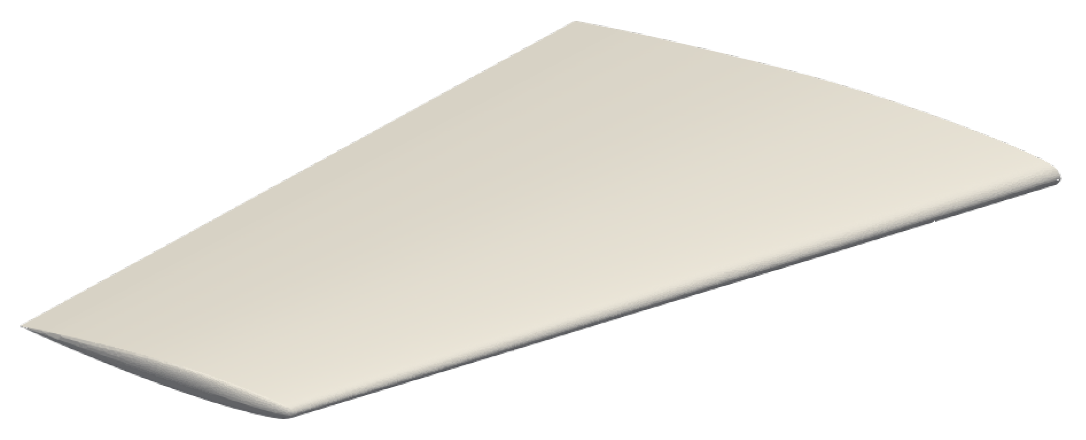
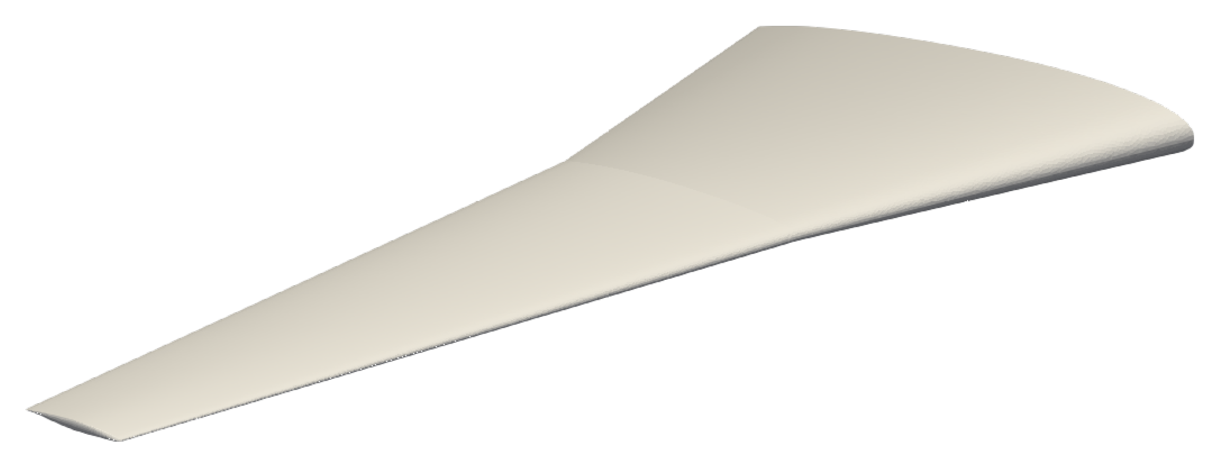
In the present work, the different models used in aircraft design, based on the linear and nonlinear potential equations as well as on the Euler and Reynolds-Averaged Navier–Stokes equations, are systematically compared on two benchmark wings. The first is the Onera M6 wing [26], a rigid and widely used transonic test case, and the second is the Embraer Benchmark Wing, which is elastic and more representative of an airliner wing. The differences in predicted aerodynamic loads and wing deflections, as well as in convergence characteristics and computational cost are analyzed, with the aim of identifying the fastest method yielding consistent and reliable results. The present work is organized as follows. In Section 2, the equations used for aerodynamic and structural modeling are briefly presented. The solvers used to carry out the calculations are also briefly described. The different fluid models are then used to solve transonic flow conditions on two rigid benchmark wings in Section 3. The resulting aerodynamic load predictions and related computational costs are compared. Section 4 is dedicated to a similar comparison but on an elastic wing. Finally, the results are summarized and discussed in Section 5 and future work is suggested.

2. Methodology

Five levels of fidelity are considered for the aerodynamic modeling: the Reynolds-Averaged Navier–Stokes equations, the Euler equations, the Full Potential equation, on its own or coupled to the Boundary Layer equations, and the Linear Potential equation. The structural dynamics is modeled using linear finite element analysis and the analysis performed in either physical or modal coordinates.

2.1. Flow Modeling

The different aerodynamic models, their abbreviations, and the corresponding software packages are detailed in

Table 1. Naming convention and equations solved in the present work.

Name	Solver	Equations
PAN	Panair	Linear Potential
NAS	NASTRAN	Linear Potential
NASC	NASTRAN	Linear Potential corrected by Euler
TRN	Tranair	Full Potential
FLO	Flow	Full Potential
SU2	SU2	Euler
TRNV	Tranair	Full Potential and Boundary Layer
SU2V	SU2	Reynolds-Averaged Navier–Stokes

.

2.1.1. High Fidelity

The unsteady Reynolds-Averaged Navier–Stokes equations can be written as

$$\frac{\partial \mathbf{U}}{\partial t}+\nabla ·{\mathbf{F}}^{\mathrm{c}}-\nabla ·{\mathbf{F}}^{\mathrm{d}}=0,$$

(1)

where $\mathbf{U}$ is the vector of the conservative flow variables defined as

$$\mathbf{U}=\left[\begin{array}{c}\rho \\ \rho \mathbf{u}\\ \rho E\end{array}\right].$$

(2)

The convective fluxes ${\mathbf{F}}^{\mathrm{c}}$ and the diffusive fluxes ${\mathbf{F}}^{\mathrm{d}}$ are defined as

$${\mathbf{F}}^{\mathrm{c}}=\left[\begin{array}{c}\rho \mathbf{u}\\ \rho \mathbf{u}\otimes \mathbf{u}+p\mathbf{I}\\ \rho E\mathbf{u}+p\mathbf{u}\end{array}\right],{\mathbf{F}}^{\mathrm{d}}=\left[\begin{array}{c}.\\ \mathit{\tau }\\ \mathit{\tau }·\mathbf{u}+{\mu }^{☆}{c}_p\nabla T\end{array}\right]$$

(3)

where $\rho$ is the density, $\mathbf{u}$ is the velocity vector, p is the pressure, E is the total energy per unit mass, $c_p$ is the specific heat capacity at constant pressure, and T is the temperature. The stress tensor for a Newtonian fluid is given by

$$\mathit{\tau }=\mu \left(\nabla \mathbf{u}+\nabla {\mathbf{u}}^{\mathrm{T}}-\frac{2}{3}\mathbf{I}\nabla ·\mathbf{u}\right).$$

(4)

The total viscosity $\mu$ and ${\mu }^{☆}$ in Equations (3) and  (4) can be expressed as

$$\begin{array}{cc}\hfill \mu & ={\mu }_{\mathrm{d}}+{\mu }_{\mathrm{t}},\hfill \\ \hfill {\mu }^{☆}& =\frac{{\mu }_{\mathrm{d}}}{{\mathrm{Pr}}_{\mathrm{d}}}+\frac{{\mu }_{\mathrm{t}}}{{\mathrm{Pr}}_{\mathrm{t}}},\hfill \end{array}$$

(5)

where $\mathrm{Pr}$ is the Prandtl number. The subscript $\mathrm{d}$ refers to dynamic quantities, which are properties of the fluid, while the subscript $\mathrm{t}$ refers to turbulent quantities, which are given by a turbulence model. In the present study, the Spalart–Allmaras model [27], commonly used for aeronautical flows, was used. The system of equations needs to be closed with the state equations

$$\begin{array}{cc}\hfill E& =c_{v}T+\frac{1}{2}\rho u^2,\hfill \\ \hfill p& =\rho RT,\hfill \end{array}$$

(6)

where u is the norm of the velocity vector, $c_v$ is the specific heat capacity at constant volume, and R is the ideal gas constant. The Euler equations are the inviscid counterpart of the Navier–Stokes equations and are obtained by neglecting the diffusive fluxes, ${\mathbf{F}}^{\mathrm{d}}$, in Equation (1).

In the present study, the Reynolds-Averaged Navier–Stokes and Euler equations were solved using SU2 [28,29,30], an open-source code for multiphysics simulations and design optimization. The equations are spatially discretized on an unstructured dual-grid using a finite volume method with a cell-vertex based approach and a second-order accurate Jameson–Schmidt–Turkel scheme. The fluxes are reconstructed using a Green–Gauss procedure. The time dependent terms are discretized using an Euler implicit scheme, and steady state is reached through a time marching procedure. For the Navier–Stokes computations, the Courant–Friedrich–Levy number is kept close to 1 and no multigrid is used, while, for the Euler computations, the condition number is set to 5 and a multigrid with a W pattern and 3 coarsening levels are used.

2.1.2. Medium Fidelity

The steady Full Potential equation assumes that the fluid is inviscid and the flow steady and isentropic. The flow is irrotational and the velocity derives from a potential $\varphi$ such that,

$$\mathbf{u}=\nabla \varphi .$$

(7)

Conservation of momentum is automatically satisfied and only the mass conservation remains, namely

$$\nabla ·\left(\rho \nabla \varphi \right)=0,$$

(8)

where the density $\rho$ is given by the isentropic flow relationship

$$\rho ={\rho }_{\infty }{\left[1+\frac{\gamma -1}{2}{M}_{\infty }^2\left(1-{\left|\nabla \varphi \right|}^2\right)\right]}^{\frac{1}{\gamma -1}},$$

(9)

where ${\rho }_{\infty }$ is the freestream density, $\gamma$ is the heat capacity ratio, and $M_{\infty }$ is the freestream Mach number. Note that the velocity has been normalized by the freestream velocity. The isentropicity assumption restricts the use of the equation to transonic flow with embedded weak shocks only. The Kutta condition must be enforced to allow a potential (irrotational) flow to generate aerodynamic loads. Mathematically, the pressure on the upper and lower sides of the trailing edge of a wing are imposed to be equal. Numerically, the potential is discontinuous across a wake extending from the trailing edge of any lifting configurations to the downstream boundary, and the Kutta condition is enforced by prescribing the continuity of the mass flux and velocity magnitude on both sides of the wake such that

$$\begin{array}{cc}\hfill [[\rho \nabla \varphi ]]& =0,\hfill \\ \hfill [[{|\nabla \varphi |}^2]]& =0,\hfill \end{array}$$

(10)

where the double squared bracket indicates a jump through the wake surface. The exact implementation of this boundary condition depends on the method used to discretize the potential equation and on the grid type. Finite volume implementations of the Kutta condition include those of Neel [31], Liegl [32], and Lyu et al. [33], while finite element formulations can be found in the works of Nishida [34], Galbraith et al. [35], and Crovato et al. [36].

In the present work, the Full Potential equation was solved using Tranair [37,38] and Flow [36,39]. Tranair is a commercial software for aircraft design and optimization developed by NASA and Boeing in the last two decades of the 20th century and distributed by Calmar Research [40] since 2004. The equation is discretized with finite elements on a rectangular Cartesian grid refined automatically by the software with an Octree method using a solution adaptation procedure. The equation is solved with a Quasi-Newton procedure combined with the Rose and Bank line search [41]. Tranair also offers the possibility to model the effect of the boundary layer on body surfaces by coupling the inviscid solution to an integral solution of the Boundary Layer equations. Details about the formulation can be found in several works by Drela [11,42,43]. Flow is an open-source finite element code developed at the University of Liège for computing the flow around arbitrary wing-fuselage configurations for preliminary aircraft design. The Full Potential equation is discretized using Continuous-Galerkin finite elements on unstructured tetrahedral grids built automatically by gmsh [44,45]. A Newton method with a quadratic line search [46] is used to solve the resulting system of equations.

2.1.3. Low Fidelity

The Full Potential equation can be transformed into an integral equation by integrating Equation (8) and using Green’s third identity. The resulting expression can then be linearized, such that

$$\varphi ={\varphi }_{\infty }-{\int }_S\left[\nabla \varphi ·\mathbf{n}K-\varphi \mathbf{n}·\nabla K\right]dS,$$

(11)

where ${\varphi }_{\infty }$ is the freestream potential, K is a kernel function depending on the geometry and the freestream conditions, and $\mathbf{n}$ is the outward unit vector normal to the surface S of the geometry. The terms appearing in the integral of Equation (11) represent the linear part of the flow, and are expressed with sources and doublets, which are fundamental solutions of the equation.

In the present study, Equation (11) was solved using Panair [47,48] and NASTRAN [49,50]. Panair is a high-order Panel Method developed at NASA during the 1980s. The body is discretized using first-order source and second-order doublet panels, allowing Panair to account for both the thickness and camber of a body with relatively few panels. The impermeability boundary condition, applied at the center of each panel, allows computing the singularity strengths from which the potential can be recovered. NASTRAN is distributed by MSC Software and uses the doublet-lattice method to solve the integral potential equation. The mean plane surface of a lifting configuration is discretized into a flat sheet containing panels with constant doublet line segments at their quarter chords, and the impermeability condition is imposed at the three quarter-chord of each panel. As a result, the doublet-lattice approach ignores the thickness and camber of the body, but  NASTRAN offers the possibility to apply corrections using geometric, numerical or experimental data [51,52]. In the present work, the Euler solution obtained with SU2 is used to build the FA2J matrix required by NASTRAN to correct the doublet-lattice pressure loads.

2.2. Structural Modeling

Neglecting internal damping, the equilibrium equations of a solid are obtained by balancing the inertial and internal forces in the solid with the external forces applied onto it. The structural equations can be written as

$${\rho }_{\mathrm{s}}\frac{d^2{\mathbf{u}}_{\mathrm{s}}}{d{t}^2}-\nabla ·\mathit{\sigma }=\mathbf{f},$$

(12)

where ${\rho }_{\mathrm{s}}$ is the solid density, $\mathit{\sigma }$ is the stress tensor, $\mathbf{f}$ are the external forces, and ${\mathbf{u}}_{\mathrm{s}}$ are the displacements. In the present work, the wing is made of a composite material modeled as orthotropic and Equation (12) is solved by the linear finite element method implemented in NASTRAN [52].

The displacements of the solid can be expressed in modal space and discretized as

$${\mathbf{u}}_{\mathrm{s}}=\mathsf{\Phi }\mathbf{q},$$

(13)

where $\mathbf{q}$ are the modal coordinates of the solid and $\mathsf{\Phi }$ is the modal matrix, containing the mode shapes of the solid. By neglecting the time dependent terms, Equation (12) can be further discretized into

$${\mathbf{K}}_{\mathrm{q}}\mathbf{q}=-{\mathbf{f}}_{\mathrm{q}},$$

(14)

where ${\mathbf{K}}_{\mathrm{q}}$ is the modal stiffness matrix and ${\mathbf{f}}_{\mathrm{q}}$ is the vector of modal forces, obtained by multiplying the vector of forces by the mode shape matrix. In the present study, the linear Equation (14) was solved by modali, an in-house modal solver [53].

2.3. Fluid–Structure Coupling

Fluid structure interaction coupling was performed using NASTRAN, an in-house MATLAB [54] code, or CUPyDO [55,56,57], depending on the software used to calculate the aerodynamic loads. The NASTRAN computations were performed by means of the elastic trim analysis, also known as SOL 144, which projects the loads directly on the structural model. Fluid structure computations were also carried out in MATLAB, such that the displacements were obtained using a MATLAB version of modali, while the loads were computed by Panair. MATLAB interpolation functions were used to transfer data between the fluid and structural meshes. The loads and the displacements were updated until the FSI process converged. Finally, Flow and SU2 were coupled to modali through CUPyDO, a Python suite designed to couple staggered solvers. The code is developed at the University of Liège and offers different coupling algorithms and different methods to interpolate the loads on the structural mesh and the displacements on the fluid nodes. In the present study, the fluid–structure computations were performed using the Block–Gauss–Seidel algorithm and the quantities were interpolated using Radial Basis Functions.

3. Rigid Aerodynamic Cases

The different fluid models and methods were first compared on the Onera M6 and Embraer Benchmark wings, making the assumption that both are rigid.

3.1. Onera M6 Wing

The wing model is depicted in Figure 1 and its geometric parameters are given in

Table 2. Geometrical properties of the Onera M6 wing.

Parameter	Value
Aspect ratio	$3.8$
Taper ratio	$0.56$
Sweep angle	${30}^{\circ }$
Root chord	805 mm
Semi-span	1196 mm

. Wind tunnel measurements are available [26] for this wing at a Mach number M of $0.839$ and an angle of attack $\alpha$ of ${3.06}^{\circ }$. The present simulations used the same flight condition and angle of attack.

A surface grid made of rectangular surface panels was used in Panair and NASTRAN. In Tranair, the wing was enclosed in a box-shaped computational domain with boundaries placed two chord lengths away from the wing in the chordwise and normal directions, and a half-span length from the wingtip in the spanwise direction. The final grid, built automatically by Tranair, consists of hexahedral cells with a minimum size of $1/200$ of the chord at the shock and leading edge. In Flow, the wing was enclosed in a box-shape computational domain with boundary faces placed $3.5$ chord lengths away from the wing in the chordwise and normal directions, and one span length away from the wingtip in the spanwise direction. The unstructured grid was built using gmsh and is made of tetrahedral cells having a characteristic size of $1/200$ and $1/100$ of the local chord at the leading edge and at the trailing edge, respectively. The inviscid SU2 grids were also built with gmsh, based on an unstructured O-grid topology extending 50 root chords away from the wing. The mesh has a characteristic cell size of $1/200$ and $1/100$ of the local chord at the leading edge and at the trailing edge, respectively. The viscous SU2 grids were built with ANSYS ICEM [58] using a multiblock structured C-grid topology extending 50 root chords away from the wing. The grid has 150, 75, and 25 hexahedra in the chordwise, normal, and spanwise directions, respectively. Experimental results consist of surface pressures measured at 271 locations distributed on seven spanwise sections, and were gathered by Schmitt and Charpin [26].

A convergence study was performed to find a suitable mesh size for each model.

Table 3. Aerodynamic coefficients obtained on several meshes with the different numerical models for the Onera M6 wing at Mach $0.839$ and angle of attack $3.{06}^{\circ }$.

Model	n. Cells	${\mathit{C}}_{\mathit{L}}$	${\mathit{C}}_{\mathit{D}}$
	360	$0.246$	$0.0055$
PAN	1000	$0.247$	$0.0047$
	1440	$0.247$	$0.0045$
	125	$0.258$	-
NAS	500	$0.248$	-
	2000	$0.245$	-
	$50,000$	$0.272$	$0.0137$
TRN	$500,000$	$0.288$	$0.0111$
	$1,000,000$	$0.288$	$0.0111$
	$110,000$	$0.287$	$0.0116$
FLO	$590,000$	$0.294$	$0.0110$
	$900,000$	$0.294$	$0.0111$
	$140,000$	$0.281$	$0.0146$
SU2	$510,000$	$0.286$	$0.0130$
	$1,200,000$	$0.287$	$0.0129$
	$300,000$	$0.257$	$0.0220$
SU2V	$1,500,000$	$0.272$	$0.0181$
	$3,000,000$	$0.270$	$0.0183$

shows the convergence for the lift and drag coefficients of the Onera M6 wing at $M=0.839$ and $\alpha =3.{06}^{\circ }$ for the different models. Note that the grids required for NASC and TRNV are similar to those used for NAS and TRN, respectively. In addition, note that NASTRAN does not provide any value for the drag coefficient. In each case, the selected grid is the one for which the results did not change significantly when the number of cells was increased, which is the medium grid indicated in Table 3.

3.1.1. Aerodynamic Loads

The angle of attack of the wing and the aerodynamic force coefficients, obtained by integrating the forces on the surface of the wing, are given in

Table 4. Aerodynamic coefficients obtained by different levels of fidelity for the Onera M6 wing at Mach $0.839$ and angle of attack $3.{06}^{\circ }$.

Model	${\mathit{C}}_{\mathit{L}}$	${\mathit{C}}_{\mathit{D}}$	${\mathit{C}}_{\mathit{M}}$
PAN	$0.247$	$0.0047$	$-0.181$
NAS	$0.248$	-	$-0.181$
NASC	$0.271$	-	$-0.201$
TRN	$0.288$	$0.0111$	$-0.212$
FLO	$0.294$	$0.0110$	$-0.217$
SU2	$0.286$	$0.0130$	$-0.212$
TRNV	$0.255$	$0.0161$	$-0.181$
SU2V	$0.272$	$0.0181$	$-0.196$

. The reference point for the moment computation is taken at the leading edge of the root chord. As expected, the nonlinear inviscid models TRN, FLO, and SU2 tend to predict higher lift and moment coefficients and a lower drag coefficient compared to the viscous models TRNV and SU2V because they ignore the boundary layer, which modifies the pressure distribution and produces shear forces. Compared to the nonlinear inviscid models, the linear models PAN and NAS slightly underestimate the lift and moment coefficients. PAN also strongly underestimates the drag coefficient, as it cannot compute the wave drag produced by shock waves. When corrected by an Euler solution, NASC predictions move closer to the results of the nonlinear models, except for the drag coefficient, which is not computed.

Figure 2 shows the pressure distribution along the mean aerodynamic chord of the wing. Note that the difference in pressure distribution between the suction and pressure sides is used to compare linear models, since NAS and NASC are based on a lattice approach, hence not accounting for the wing’s thickness. Because of their underlying assumptions, PAN and NAS are unable to predict shocks and to represent the actual physics of transonic flows. Since NASC is corrected using an Euler calculation, it is the only linear approach that captures the shock. The nonlinear inviscid models TRN, FLO, and SU2 were found to correctly represent the physics even though they predict a stronger shock when compared to the experimental results. Finally, the viscous models TRNV and SU2V give accurate pressure distribution predictions, although a small difference in the shock location and strength is still observed between them.

Figure 2b also shows that the different numerical solution procedures implemented in Flow and Tranair slightly affect the shock strength and location. Moreover, in the case of viscous models (Figure 2c), the difference in boundary layer and turbulence modeling also affects the solution. This has a direct impact on the aerodynamic coefficients: SU2 tends to predict higher values of drag compared to TRN and FLO, while TRNV tends to underestimate the lift, moment, and drag coefficients compared to SU2V, as illustrated in Table 4.

Figure 3 shows the distribution of the sectional lift and moment coefficients along the span of the Onera M6 wing, obtained by integrating numerically the pressure coefficient in the chordwise direction. The sectional moment is computed around the local quarter-chord. The lift distribution predicted by the different solvers is similar to the experimental measurements, but there are differences in magnitude. In particular, as already noted in Table 4, the nonlinear inviscid models tend to predict higher lift coefficients for the same angle of attack. Both the inviscid and viscous nonlinear models predict sectional moment distributions that are similar to the experimental results. Since inviscid models ignore the boundary layer and predict stronger shocks, they tend to yield higher magnitudes for the moment coefficient. Finally, the moment distribution predicted by the linear models does not follow the same trend as the experimental data, except when correct by a nonlinear solution.

3.1.2. Computing Performance

Models PAN, NAS, NASC, TRN, FLO, and TRNV were run in serial on a laptop fitted with an Intel i7-7700HQ processor ($2.8$ GHz), and models SU2 and SU2V were run on a cluster equipped with Intel Xeon X5650 processors ($2.7$ GHz). The mesh sizes and computational times are given in

Table 5. Mesh size and computational time required by the different models for the Onera M6 benchmark case.

Model	n. Cells	n. Threads	Wall-Clock Time	Cpu Time
PAN	1000	1	10 s	10 s
NAS	500	1	20 s	20 s
NASC	500	1	20 s	20 s
TRN	$500,000$	1	7 min	7 min
FLO	$590,000$	1	13 min	13 min
SU2	$510,000$	12	14 min	3 h
TRNV	$500,000$	1	15 min	15 min
SU2V	$1,500,000$	36	24 h	36 d

. The linear models PAN, NAS, and NASC are very fast since they require only one iteration to solve a scalar equation and need a small number of cells. Note that the computational time needed to compute the reference Euler solution required by NASC is not taken into account. On the other hand, the higher-fidelity models SU2 and SU2V need many iterations to solve five and six equations, respectively, which makes them slower. The medium-fidelity models TRN, FLO, and TRNV require few Newton iterations to solve a scalar equation, for a typical runtime of 10 min.

Table 5 shows that SU2V is quite slow. This is mainly due to the fact that using acceleration techniques such as Courant–Friedrich–Levy number adaptation or multigrid was not possible for this computation. Note that the goal of the present work is to identify the trends in the computational cost of the different models. Optimizing the numerical parameters of the different solvers could lead to a decrease in computational time.

3.2. Embraer Benchmark Wing

The different models were next applied to the Embraer Benchmark wing, which is more representative of a transport aircraft wing. The wing model is depicted in Figure 4 and its approximated geometrical parameters are provided in

Table 6. Geometrical properties of the Embraer Benchmark wing.

Parameter	Value
Aspect ratio	10
Taper ratio	$0.28$
Sweep angle	${26}^{\circ }$
Dihedral angle	$5^{\circ }$

. This benchmark is purely numerical and no experimental data are available for this case. As such, the numerical results are compared to the highest aerodynamic level of fidelity used in the present work: the RANS equations. The wing was simulated at Mach number $0.78$ and altitude of $27,000$ ft. For each calculation, the angle of attack was adjusted such that the resulting lift coefficient was equal to $C_L=0.60$. Note that this procedure was automatically handled by the solver for models TRN and TRNV.

The models for the different solvers were built in the same way as for the Onera M6 case, but the grid sizes differed. Again, a convergence study was performed on each of the meshes. PAN and NAS/NASC werediscretized with 1400 and 800 surface panels, respectively. The final grids of TRN and TRNV consist of $500,000$ hexahedral cells, with a minimum cell size of $1/200$ of the chord at the shock and leading edge. The mesh used for FLO consists of $660,000$ tetrahedral cells, with a characteristic size of $1/100$ of the local chord at the leading and trailing edges. The unstructured grid used for SU2 contains $1.3$ million tetrahedra with characteristic cell sizes of $1/200$ and $1/100$ of the local chord at the leading edge and at the trailing edge, respectively. Finally, the grid for SU2V contains 150, 75, and 25 cells in the chordwise, normal, and spanwise direction, respectively, for a total of $1.5$ million hexahedra.

3.2.1. Aerodynamic Loads

The computed angle of attack of the wing and the resulting aerodynamic force coefficients, obtained by integrating the forces on the surface of the wing, are given in

Table 7. Aerodynamic coefficients obtained by different levels of fidelity for the rigid Embraer Benchmark Wing at Mach $0.78$ and lift coefficient $0.60$.

Model	$\mathit{\alpha }{(}^{\circ })$	${\mathit{C}}_{\mathit{L}}$	${\mathit{C}}_{\mathit{D}}$	${\mathit{C}}_{\mathit{M}}$
PAN	$-0.5$	$0.60$	$0.0136$	$-0.866$
NAS	$+5.3$	$0.60$	-	$-0.739$
NASC	$-1.1$	$0.60$	-	$-0.872$
TRN	$-0.9$	$0.60$	$0.0159$	$-0.857$
FLO	$-0.8$	$0.60$	$0.0147$	$-0.853$
SU2	$-0.9$	$0.60$	$0.0167$	$-0.866$
TRNV	$+0.2$	$0.60$	$0.0241$	$-0.815$
SU2V	$+0.4$	$0.60$	$0.0244$	$-0.819$

. TRNV and SU2V require a higher angle of attack to reach the same target lift than the inviscid models. They also predict higher values for the drag coefficient and moment coefficients. Linear models fall into two categories. On the one hand, PAN, which makes use of the full geometry of the wing, predicts a slightly higher angle of attack and a lower value of the drag coefficient when compared to TRN, FLO, and SU2. On the other hand, NAS is based on a flat lattice geometry and predicts a significantly higher angle of attack. Predictably, when the pressure correction calculated from the Euler solution is used, NASC predicts almost the same results as the nonlinear solvers.

Figure 5 shows the pressure distribution along the mean aerodynamic chord of the Embraer Benchmark Wing at a lift coefficient of $0.6$. PAN predicts a similar pressure difference compared to that obtained from SU2V, except at the shock and pressure peak locations. NAS strongly overpredicts the pressure peak at the leading edge. This is mostly due to the high angle of attack needed to achieve the target lift coefficient. While PAN and NAS are not able to capture the shock, NASC is corrected by an Euler solution and the resulting difference in pressure is comparable to that calculated by SU2V, except that the shock is stronger and located further downstream. The same is true for the results obtained from the inviscid nonlinear solvers, which also feature a reduced pressure peak compared to the SU2V result. As opposed to the Onera M6 case, the shock on the Embraer wing is weaker and FLO was found to smear the shock and underestimate the drag compared to TRN and SU2. TRNV, found to be as accurate as SU2V in the Onera M6 case, predicts a stronger shock and a slightly higher drag coefficient in the present case.

Figure 6 shows the sectional lift and moment coefficients distribution along the span of the Embraer wing at a lift coefficient of $0.6$. In this case, where the lift coefficient of the wing is prescribed, the lift and moment distributions predicted by the various models are similar, with the following exceptions. Firstly, as in the Onera M6 case, inviscid models tend to predict moment coefficients with higher magnitude. Secondly, PAN does not capture the dip in the moment distribution located at the kink of the wing ($y/b=0.37$). Thirdly, NAS yields highly inaccurate results for the angle of attack, pressure, lift, and moment distributions. It should be recalled that the Embraer wing is cambered while the Onera M6 is not. NASTRAN does not include camber in its calculation by default; a camber or pressure correction must be applied. The pressure correction obtained here from an Euler computation improves all predictions significantly, as shown by the NASC results.

3.2.2. Computing Performance

The same computers were used as for the Onera M6 wing. The mesh size and the computational time are given in

Table 8. Mesh size and computational time required by the different models for the Embraer benchmark case.

Model	n. Cells	n. Threads	Wall-Clock Time	Cpu Time
PAN	1400	1	10 s	10 s
NAS	800	1	25 s	25 s
NASC	800	1	25 s	25 s
TRN	$500,000$	1	8 min	8 min
FLO	$660,000$	1	16 min	16 min
SU2	$1,300,000$	12	30 min	6 h
TRNV	$500,000$	1	42 min	42 min
SU2V	$1,500,000$	60	48 h	120 d

. Again, the computational time needed to compute the reference Euler solution required by NASC is not taken into account. Compared to the Onera M6 wing, the Embraer wing has a higher aspect ratio and unstructured meshes need to be denser to achieve the same resolution. This has an impact on the runtime: FLO is now two times slower than TRN and two orders of magnitude slower than the linear models. Furthermore, SU2 is about 50 times slower than TRN. As in the Onera M6 case, TRNV is significantly faster than SU2V. Overall, the linear models PAN, NAS, and NASC remain very fast, while higher-fidelity SU2 and SU2V based on the Euler and Navier–Stokes equations are significantly slower. The full potential models TRN, FLO, and TRNV offer a good tradeoff between accuracy and computational time.

3.3. Discussion

For both the test cases considered in the present work, the presence of the shock and the boundary layer affected the results significantly. The shock was found to change the behavior of the pressure distribution and to impact the lift, drag, and moment coefficients. On the other hand, the boundary layer was found to affect both the shock location and its strength, which in turn affected the aerodynamic coefficients. Moreover, accounting for the shear stresses significantly increases the magnitude of the drag coefficient. These results are in line with, and support, those previously reported by various authors [7,8,9,11,12,13]. Results also show that using lattice methods, which do not account for the wing thickness and camber, can have a significant impact on the solution. Correcting such methods with a nonlinear solution improves all results except for the drag, but the computational time becomes slightly higher than the one needed to obtain the nonlinear solution. This observation supports the early suggestion of Verhoff and O’Neil [3], which is widely accepted today albeit in the absence of thorough validation, of using multi-fidelity modeling for transonic flow computations.

The results presented up to this point demonstrate that, in the presence of shocks, linear methods predict lift with reasonable accuracy but underestimate drag and pitching moment and yield unphysical pressure distributions. They are therefore not suited for transonic aerodynamic computations and optimization in preliminary aircraft design. On the other hand, the Euler and Reynolds-Averaged Navier–Stokes equations correctly capture the physics but have a high computational cost. Full potential models were found to give reliable results for a moderate computational cost. More particularly, the full potential equation was found to predict results comparable to the Euler equations for less than a tenth of the computational cost. Note that, even though the shock on the Onera M6 is relatively strong, the full potential results remain accurate and the formulation does not breakdown, contrary to what may sometimes be reported in the literature [14,15]. When coupled to the boundary layer equations, the full potential computations are almost as accurate as Navier–Stokes results for less than a thousandth of the computational cost.

4. Static Aeroelastic Case

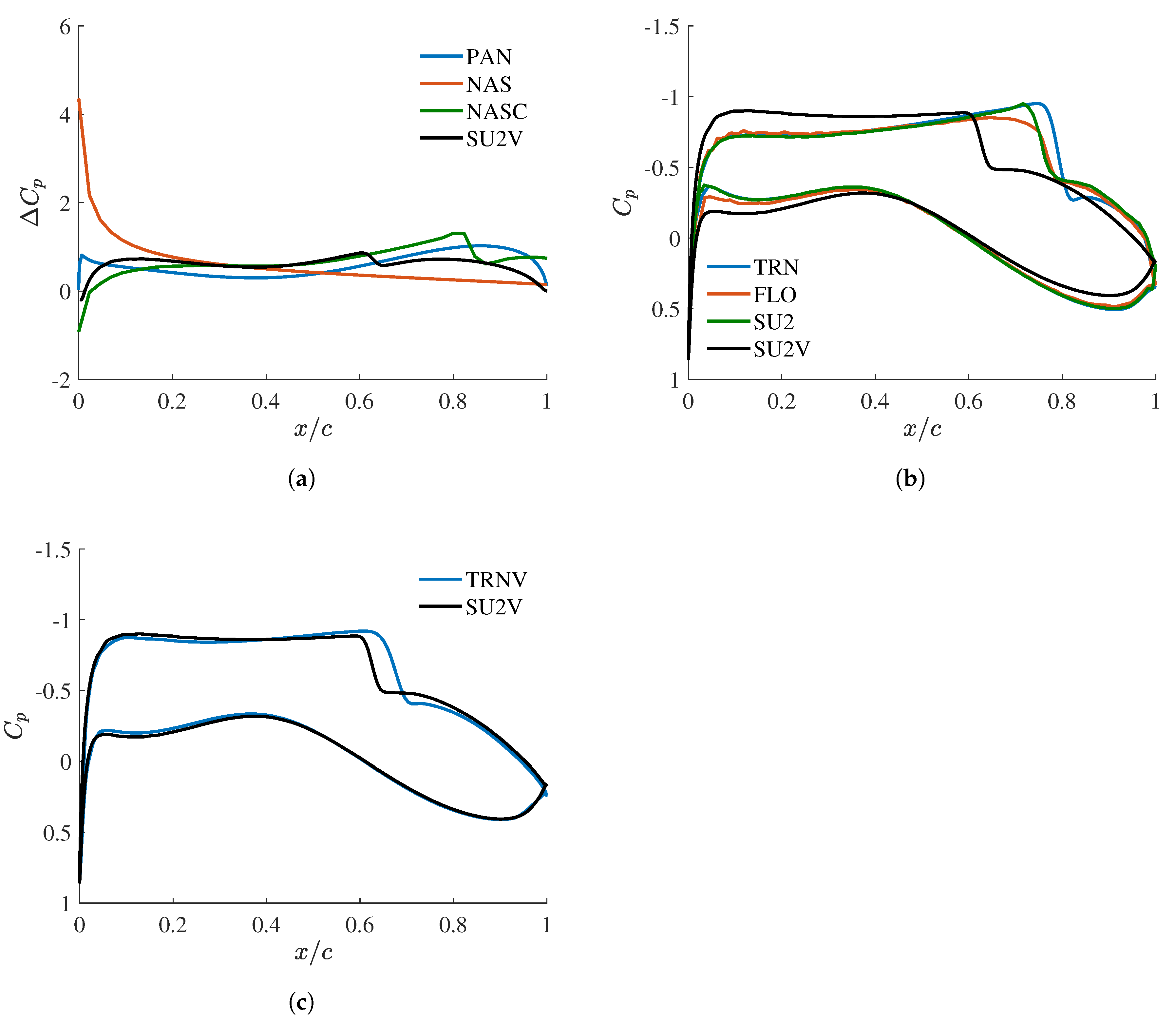
In this section, models PAN, NAS, NASC, FLO, and SU2 are compared on the flexible Embraer Benchmark Wing, which is analyzed in the context of a static fluid–structure interaction simulation. The objective is to predict the deformed shape of the wing subjected to the flight condition described in Section 3.2 and to recover the new angle of attack needed to obtain a lift coefficient of $0.6$, as well as the new load distributions along the span. Note that the wing is clamped at its root to represent its attachment to the fuselage. Such a boundary condition is not fully realistic as the fuselage is not rigid. However, this setup allows comparing the different solvers.

The aerodynamic meshes used by all the models are those described in Section 3.2. The associated structural model was discretized in NASTRAN and consists of $50,000$ shell elements. The fluid–structure computations for NAS and NASC were carried out directly within NASTRAN using the elastic trim analysis. The other aerodynamic models were coupled to a structural model, obtained by a modal decomposition performed in NASTRAN. The mesh used by the modal solver consists of 2100 points distributed on the surface of the wing. Note that these points were only used to create the modal matrix to transfer quantities between the physical and modal spaces. FLO and SU2 were coupled to the modal solver using CUPyDO while PAN was coupled through MATLAB. The fluid–structure computation stopped when the difference in an objective function between two consecutive iterations fell below a given tolerance. In CUPyDO, the objective function includes the displacements, while the loads are considered in MATLAB. In both cases, a normalized tolerance of ${10}^{-4}$ was used.

4.1. Aerodynamic Loads

Table 9. Angles of attack and aerodynamic coefficients for the flexible Embraer wing at Mach $0.78$ and lift coefficient $0.60$ obtained from different levels of fidelity.

Model	$\mathit{\alpha }$ (${}^{\circ }$)	${\mathit{C}}_{\mathit{L}}$	${\mathit{C}}_{\mathit{D}}$	${\mathit{C}}_{\mathit{M}}$
PAN	$+0.5$	$0.60$	$0.0148$	$-0.885$
NAS	$+6.1$	$0.60$	-	$-0.705$
NASC	$+0.9$	$0.60$	-	$-0.812$
FLO	$+0.1$	$0.60$	$0.0141$	$-0.867$
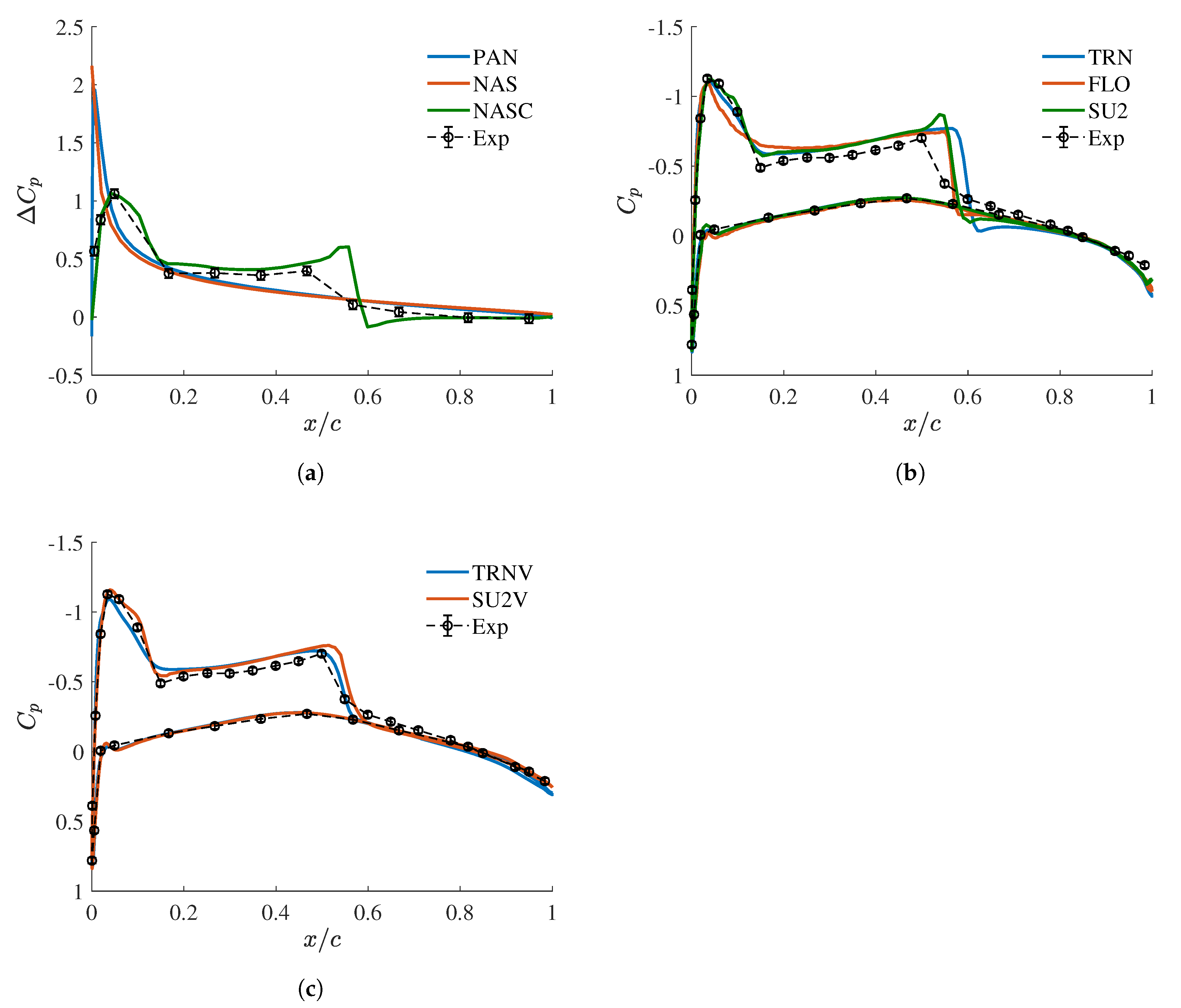
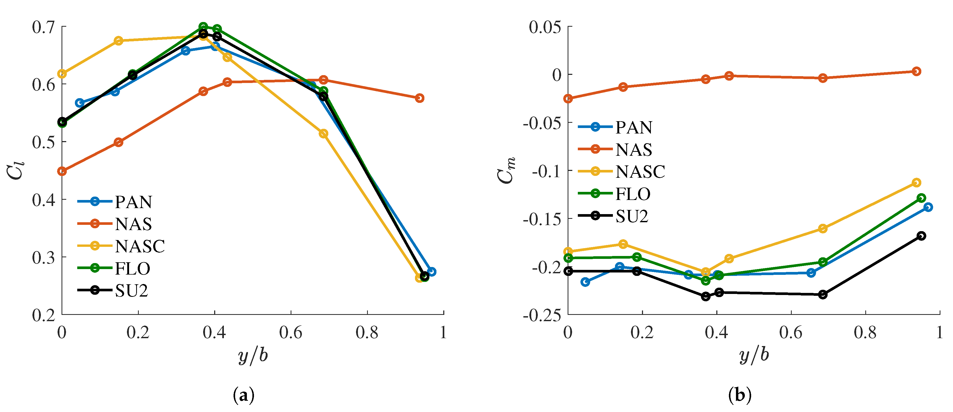
SU2	$-0.1$	$0.60$	$0.0186$	$-0.890$

summarizes the new angle of attack and aerodynamic coefficients of the benchmark wing in its deformed configuration. As in the rigid case presented in Section 3.2, the linear model PAN slightly overpredicts the angle of attack needed to achieve the target lift coefficient when compared to nonlinear models. On the other hand, the lattice model NAS neglects the camber of the wing, strongly overperdicts the angle of attack, and underpredicts the moment coefficient. Using the Euler correction with NASC significantly improves the predictions, even though the angle of attack is still overestimated by about 1 degree. In this case, FLO was also found to strongly underestimate the drag coefficient when compared to SU2. Comparing the results in Table 7 and Table 9 illustrates the impact of wing deformation on the angle of attack and aerodynamic coefficients.

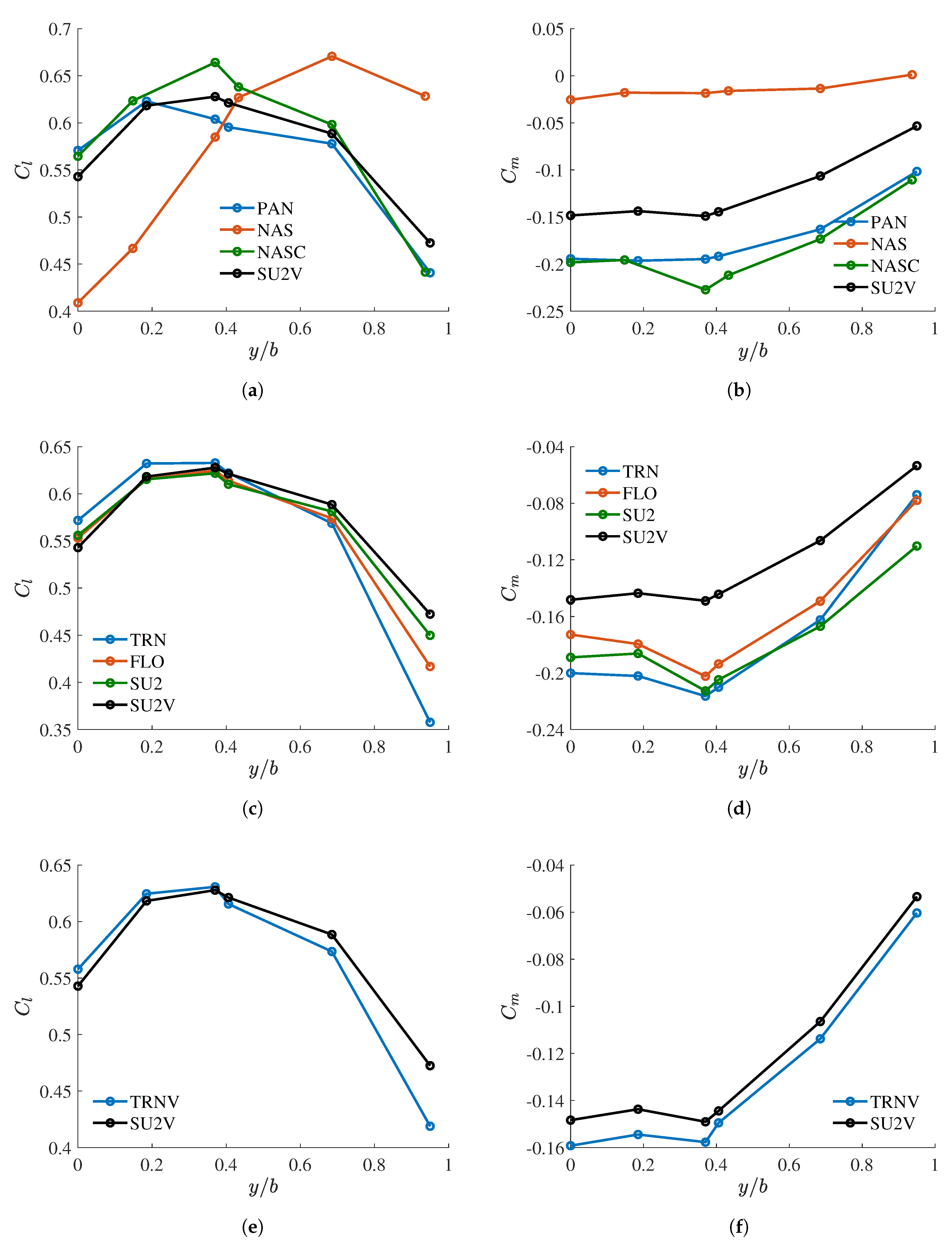
Figure 7a,b shows the lift and the quarter-chord moment coefficient distribution along the span of the deformed wing, respectively. With the exception of NAS, all models predict similar distributions for both the lift and moment. Note that, as there is no viscous solution, it is not known if the inviscid methods still underestimate the moment. Again, NAS is completely inaccurate as it ignores the camber of the wing.

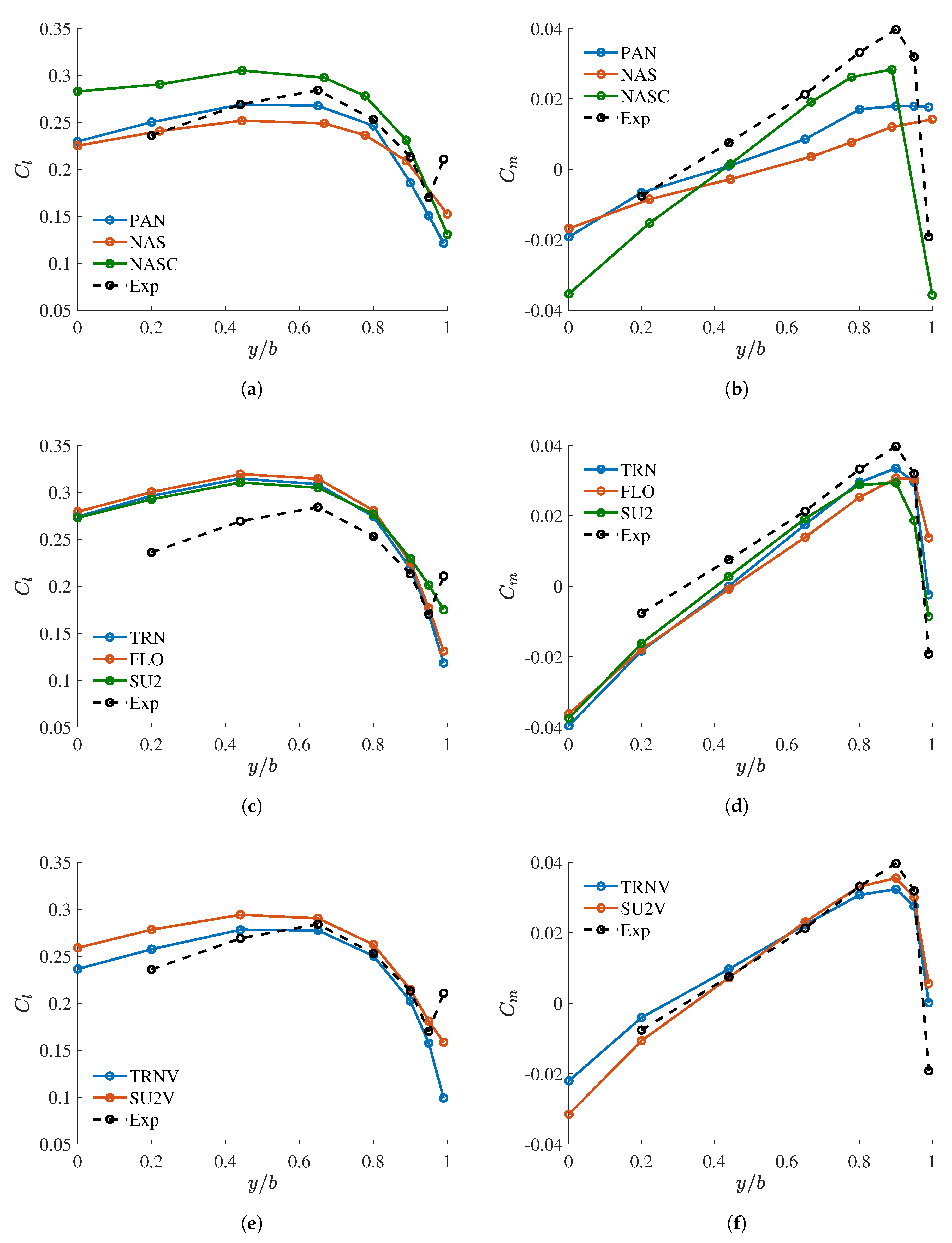
4.2. Wing Deflection

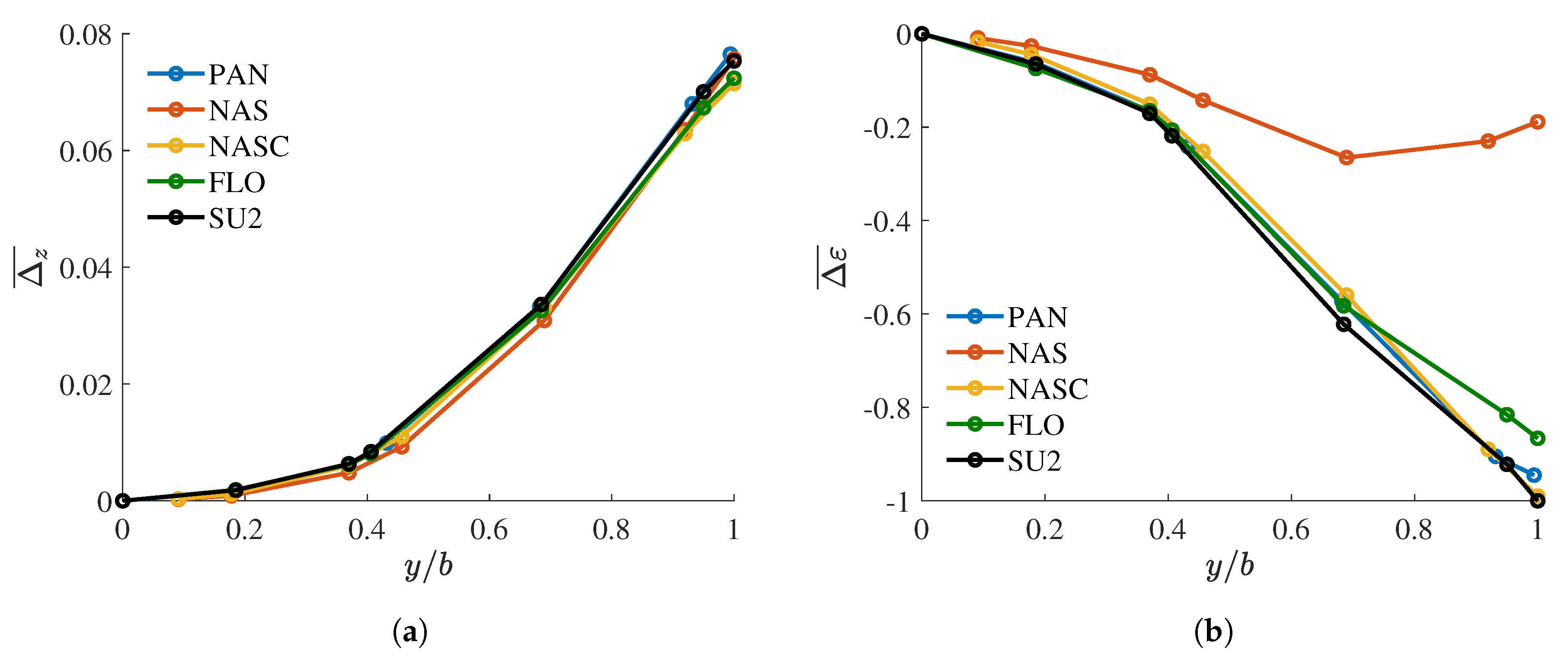
Figure 8 shows the vertical displacement, averaged between the leading and trailing edges, and the nose-up rotation along the span of the deformed wing. Note that the displacement is normalized with respect to the half-span of the wing and the rotation angle is normalized by the maximum value of the rotation. All models predict similar results for both displacement and rotation, except for NAS, which strongly underestimates rotation at the outboard section of the wing.

4.3. Computational Performance

The mesh size and the computational time required to run the computations are given in

Table 10. Mesh size and computational time required by the different models for the Embraer Benchmark Wing case.

Model	n. Cell	n. Threads	Wall-Clock Time
PAN	1400	1	90 s
NAS	800	1	75 s
NASC	800	1	6 h + 75 s
FLO	$660,000$	1	$1.5$ h
SU2	$1,500,000$	1	22 h

. The calculations were performed in serial on a laptop fitted with an Intel i7-7700HQ processor ($2.8$ GHz). In this case, the computational cost of the Euler correction required by NASC is included. PAN, FLO, and SU2 converged, respectively in nine, seven, and nine FSI iterations, while NAS and NASC converged in three iterations. PAN and NAS are more than one order of magnitude faster than FLO, which is itself more than one order of magnitude faster than SU2.

4.4. Discussion

Although panel methods do not capture shocks, their static aeroelastic predictions are, in general, quite similar to those obtained from the nonlinear solvers. For the present case at least, static wing deflections are not sensitive to shock modeling. Consequently, flight shape calculations can be carried out using linear methods with reasonable confidence in the predictions. In any case, the camber must be modeled or corrected, otherwise wildly inaccurate results will be obtained. The corrected doublet lattice model is also quite accurate but its computational cost is much higher due to the need to calculate an Euler solution.

Note that the ability of linear methods to predict wing displacements accurately seems to be quite sensitive to the geometry. Results previously reported by Romanelli et al. [21] show that the doublet lattice method was less accurate than Euler computations, especially near the wingtip. However, it is unclear whether the authors corrected the method with higher-fidelity data.

5. Conclusions

The objective of the present work is to assess systematically the impact of the aerodynamic level of fidelity on steady aerodynamic and static aeroelastic computations typically performed in preliminary aircraft design. To this end, several aerodynamic models were compared on the Onera M6 and the Embraer Benchmark wings.

The assumptions made by considering different levels of fidelity can be grouped into four categories: flow viscosity, isentropicity, linearity, and model geometry. The results obtained in the context of steady aerodynamic computations on both rigid wings illustrate that neglecting the viscosity leads to an underestimation of the aerodynamic loads, particularly the moment and the drag. When the lift coefficient is imposed, the angle of attack is underestimated by about $1^{\circ }$. The shock strength is also underestimated and its location is moved downstream. These results globally agree with those previously reported in the literature [9,13]. Considering the flow to be isentropic does not significantly affect the solution. This is particularly true for the flows considered in aircraft design, where only weak shocks are present. However, the results obtained on the Onera M6 demonstrate that the full potential formulation does not necessarily break down when a relatively strong shock is present, although this statement raises the question of what constitutes a strong shock wave and what are the exact limits of validity of the full potential theory. Further considering the flow to be fully linear has only a mild impact on the lift and the moment, even if the pressure distribution is significantly affected. The drag is also underestimated since the wave drag produced through shocks is not accounted for. Finally, modeling the wing without accounting for its camber results in a complete miscalculation of the angle of attack and aerodynamic loads.

The present analysis suggests that at least a nonlinear method is required to accurately capture transonic physics. Even though full potential methods achieve the best tradeoff between accuracy and computational cost for rigid steady computations, they are still too expensive for static aeroelastic computations in preliminary aircraft design. As such, calculations are usually performed on wings already optimized for the transonic flow regime; a linear potential method seems sufficient to predict the wing loading and deformation and should yield results similar to those obtained using nonlinear methods, except for the drag. Note, however, that this result strongly depends on the geometry, as results previously reported in the literature [21] suggest that linear methods are not necessarily accurate in transonic cases. In any case, if a linear model is used to compute the wing deflection, a single nonlinear rigid aerodynamic calculation should be performed on the deformed shape in order to estimate more accurate aerodynamic loads. This two-stage computation strategy might offer a cheaper alternative to multi-fidelity static aeroelastic computations, whereby nonlinear computations are performed during the iterative process to calibrate a linear computation. The two-stage computation could also be more accurate than correcting a linear method with higher-fidelity data obtained from a rigid aerodynamic computation performed on the undeformed wing shape.

References

1. Flightpath 2050 Europe’s Vision for Aviation. 2019. Available online: https://ec.europa.eu/transport/sites/transport/files/modes/air/doc/flightpath2050.pdf (accessed on 20 December 2019).
2. Bhateley, I.; Cox, R. Application of Computational Methods to Transonic Wing Design. In Progress in Astronautics and Aeronautics; Chapter 8; American Institute of Aeronautics and Astronautics: Reston, VA, USA, 1981; Volume 81, pp. 405–431. [Google Scholar]
3. Verhoff, A.; O’Neil, P. Extension of FLO Codes to Transonic Flow Prediction for Fighter Configurations. In Progress in Astronautics and Aeronautics; Chapter 11; American Institute of Aeronautics and Astronautics: Reston, VA, USA, 1981; Volume 81, pp. 467–487. [Google Scholar]
4. Rubbert, P.; Saaris, G. Review and evaluation of a three-dimensional lifting potential flow analysis method for arbitrary configurations. In Proceedings of the 10th AIAA Aerospace Science Meeting, San Diego, CA, USA, 17–19 January 1972. [Google Scholar]
5. Flores, J.; Barton, J.; Holst, T.; Pulliam, T. Comparison of the Full-Potential and Euler Formulations for Computing Transonic Airfoil Flows; Technical Report; NASA: Washington, DC, USA, 1984. [Google Scholar]
6. Klopfer, G.H.; Nixon, D. Nonisentropic potential formulation for transonic flows. AIAA J. 1984, 22, 770–776. [Google Scholar] [CrossRef]
7. Le Balleur, J. Strong matching methods for Computing Transonic Viscous Flow including Wakes and Seprations—Lifting airfoils. La Rech. Aerosp. 1981, 3, 161–185. [Google Scholar]
8. Melnik, R.; Chow, R.; Mead, H.; Jameson, A. A Multigrid Method for the Computation of Viscid/Inviscid Interaction on Airfoils; Technical Report; Grumman Aerospace Corporation: Bethpage, NY, USA, 1983. [Google Scholar]
9. Van Muijden, J.; Broekhuizen, A.; van der Wees, A.; van der Vooren, J. Flow analysis and drag prediction for transonic transport wing/body configurations using a viscous-inviscid interaction type method. In Proceedings of the 19th ICAS Congress, Anaheim, CA, USA, 18–23 September 1994. [Google Scholar]
10. Holst, T. Transonic flow computations using nonlinear potential methods. Prog. Aerosp. Sci. 2000, 36, 1–61. [Google Scholar] [CrossRef] [Green Version]
11. Drela, M.; Giles, M.; Thompkins, W. Newton Solution of Coupled Euler and Boundary-Layer Equations. In Numerical and Physical Aspects of Aerodynamic Flows; Chapter 7; Spinger: Berlin/Heidelberg, Germany, 1986; Volume 3, pp. 143–154. [Google Scholar]
12. Potsdam, M. An Unstructured Mesh Euler and Interactive Boundary Layer Method for Complex Configurations. In Proceedings of the 12th Applied Aerodynamic Conference, Colorado Springs, CO, USA, 20–23 June 1994. [Google Scholar]
13. Aftosmis, M.; Berger, M.; Alonso, J. Applications of a Cartesian Mesh Boundary-Layer Approach for Complex Configurations. In Proceedings of the 44th AIAA Aerospace Science Meeting and Exhibit, Reno, NV, USA, 9–12 January 2006. [Google Scholar]
14. Jameson, A. The Evolution of Computational Methods in Aerodynamics. J. Appl. Mech. 1983, 50, 1052–1070. [Google Scholar] [CrossRef]
15. Johnson, F.; Tinoco, E.; Yu, N. Thirty Years of development and applications of CFD at Boeing Commercial Airplanes, Seattle. Comput. Fluids 2005, 34, 1115–1151. [Google Scholar] [CrossRef] [Green Version]
16. Jovanov, K.; De Breuker, R. Accelerated convergence of high-fidelity aeroelasticity using low-fidelity aerodynamics. In Proceedings of the 16th International Forum on Aeroelasticity and Structural Dynamics, St. Petersburg, Russia, 28 June–2 July 2015. [Google Scholar]
17. Kenway, G.; Martins, J. Multipoint High-fidelity Aerostructural Optimization of a Transport Aircraft Configuration. J. Aircr. 2014, 51, 144–160. [Google Scholar] [CrossRef] [Green Version]
18. Brooks, T.; Kenway, G.; Martins, J. Benchmark Aerostructural Models for the Study of Transonic Aircraft Wings. AIAA J. 2018, 56, 2840–2855. [Google Scholar] [CrossRef]
19. Heeg, J.; Chwalowski, P.; Schuster, D. Overview and lessons learned from the Aeroelastic Prediction Workshop. In Proceedings of the 54th AIAA/ASME/ASCE/AHS/ASC Structures, Structural Dynamics and Materials Conference, Boston, MA, USA, 8–11 April 2013. [Google Scholar]
20. Schuster, D.; Heeg, J.; Wieseman, C.; Chwalowski, P. Analysis of Test Case Computations and Experiments for the Aeroelastic Prediction Workshop. In Proceedings of the 51st AIAA Aerospace Sciences Meeting, Grapevine, TX, USA, 7–10 January 2013. [Google Scholar]
21. Romanelli, G.; Castellani, M.; Mantegazza, P.; Ricci, S. Coupled CSD/CFD non-linear aeroelastic trim of free-flying flexible aircraft. In Proceedings of the 53rd AIAA/SME/ASCE/AHS/ASC Structures, Structural Dynamics and Materials Conference, Honolulu, HI, USA, 23–26 April 2012. [Google Scholar]
22. Acar, P.; Nikbay, M. Steady and Unsteady Aeroelastic Computations of HIRENASD Wing for Low and High Reynolds Numbers. In Proceedings of the 54th AIAA/SME/ASCE/AHS/ASC Structures, Structural Dynamics and Materials Conference, Boston, MA, USA, 8–11 April 2013. [Google Scholar]
23. Edwards, J.; Malone, J. Current status of computational methods for transonic unsteady aerodynamics and aeroelastic applications. Comput. Syst. Eng. 1992, 3, 545–569. [Google Scholar] [CrossRef] [Green Version]
24. Schuster, D.; Liu, D.; Huttshell, L. Computational Aeroelasticity: Success, Progress, Challenge. J. Aircr. 2003, 40, 843–856. [Google Scholar] [CrossRef] [Green Version]
25. Henshaw, M.D.C.; Badcock, K.; Vio, G.; Allen, C.; Chamberlain, J.; Kaynes, I.; Dimitriadis, G.; Cooper, J.; Woodgate, M.; Rampurawala, A.; et al. Non-linear aeroelastic prediction for aircraft applications. Prog. Aerosp. Sci. 2007, 43, 65–137. [Google Scholar] [CrossRef]
26. Schmitt, V.; Charpin, F. Pressure distributions on the ONERA-M6-wing at transonic Mach numbers. In Experimental Data Base for Computer Program Assessment; Report of the Fluid Dynamics Panel Working Group 04, AGARD AR 138 Office National d’Etudes et de Recherches Aerospatiales 92320: Chatillon, France, 1979; Volume 4. [Google Scholar]
27. Spalart, P.; Allmaras, S. A one equation turbulence model for aerodynamic flows. AIAA J. 1992, 94, 439. [Google Scholar]
28. Palacios, F.; Colonno, M.; Aranake, A.; Campos, A.; Copeland, S.; Economon, T.; Lonkar, A.; Lukaczyk, T.; Taylor, T.; Alonso, J. Stanford University Unstructured (SU2): An open-source integrated computational environment for multi-physics simulation and design. AIAA J. 2013. [Google Scholar] [CrossRef] [Green Version]
29. Economon, T.; Palacios, F.; Copeland, S.; Lukaczyk, T.; Alonso, J. Stanford University Unstructured (SU2): An open-source suite for multi-physics simulation and design. AIAA J. 2016. [Google Scholar] [CrossRef]
30. Stanford University Unstructured (SU2). 2019. Available online: https://su2code.github.io/ (accessed on 20 December 2019).
31. Neel, R. Advances in Computational Fluid Dynamics: Turbulent Separated Flows and Transonic Potential Flows. Ph.D. Thesis, Virginia Polytechnic Institute, Blacksburg, VA, USA, 1995. [Google Scholar]
32. Lieg, R. A Full Potential Solver for Lifting Flows on Unstructured Tetrahedral Meshes. Master’s Thesis, Concordia University, Montreal, QC, Canada, 2005. [Google Scholar]
33. Lyu, F.; Xiao, T.; Yu, X. A Fast and Automatic Full Potential Finite Volume Solver on Cartesian Grids for Unconventional Configurations. Chin. J. Aeronaut. 2017, 30, 951–963. [Google Scholar] [CrossRef]
34. Nishida, B. Fully Simultaneous Coupling of the Full Potential Equation and the Integral Boundary Layer Equations in Three Dimensions. Ph.D. Thesis, Massachussets Institute of Technology, Cambridge, MA, USA, 1996. [Google Scholar]
35. Galbraith, M.; Allmaras, S.; Haimes, R. Full Potential Revisited: A Medium Fidelty Aerodynamic Analysis Tool. In Proceedings of the 55th AIAA SciTech 2017 & Aerospace Sciences Meeting, Grapevine, TX, USA, 9–13 January 2017. [Google Scholar]
36. Crovato, A.; Boman, R.; Guner, H.; Terrapon, V.; Dimitriadis, G.; Almeida, H.; Prado, A.; Breviglieri, C.; Cabral, P.; Silva, G. A Full Potential Static Aeroelastic Solver for Preliminary Aircraft Design. In Proceedings of the 18th International Forum on Aeroelasticity and Structural Dynamics, Savannah, GA, USA, 9–13 June 2019. [Google Scholar]
37. Johnson, F.T.; Samant, S.S.; Bieterman, M.; Melvin, R.; Young, D.; Bussoletti, J.; Hilmes, C. Tranair: A Full-Potential, Solution-Adaptative, Rectangular Grid-Code for Predicting Subsonic, Transonic, and Supersonic Flows About Arbitrary Configurations; Technical Report; NASA: Washington, DC, USA, 1992. [Google Scholar]
38. Bieterman, M.; Melvin, R.; Johnson, F.; Bussoletti, J.; Young, D.; Huffman, W.; Hilmes, C.; Drela, M. Boundary Layer Coupling in a General Configuration Full Potential Code; Technical Report; The Boeing Company: Seattle, WA, USA, 1994. [Google Scholar]
39. Waves. 2019. Available online: https://gitlab.uliege.be/am-dept/waves (accessed on 20 December 2019).
40. Calmar Research. 2019. Available online: http://www.calmarresearch.com/NF/home.htm (accessed on 20 December 2019).
41. Bank, R.; Rose, D. Global Approximate Newton Method. Numer. Math. 1981, 27, 179–295. [Google Scholar] [CrossRef]
42. Drela, M. Two-Dimensional Transonic Aerodynamic Design and Analysis Using The Euler Equations. Ph.D. Thesis, Massachussets Institute of Technology, Cambridge, MA, USA, 1985. [Google Scholar]
43. Mughal, B.; Drela, M. A calculation method for the three-dimensonal boundary-layer equations in integral form. In Proceedings of the 31st AIAA Aerospace Sciences Meeting, Reno, NV, USA, 1–14 January 1993. [Google Scholar]
44. Geuzaine, C.; Remacle, J.F. Gmsh: A three-dimensional finite element mesh generator with built-in pre- and post-processing facilities. Int. J. Numer. Methods Eng. 2009, 79, 1309–1331. [Google Scholar] [CrossRef]
45. Gmsh: A Three-Dimensional Finite Element Mesh Generator with Built-In Pre- and Post-Processing Facilities. 2019. Available online: http://gmsh.info (accessed on 20 December 2019).
46. Sun, W.; Yuan, Y. Optimization Theory and Methods—Nonlinear Programming; Springer: Berlin/Heidelberg, Germany, 2006. [Google Scholar]
47. Carmichael, R.; Erickson, L. Panair: A higher order panel method for predicting subsonic or supersonic linear potential flows about arbitrary configurations. AIAA J. 1981, 7, 1255. [Google Scholar]
48. Panair. 2019. Available online: https://pdas.com/panair.html (accessed on 20 December 2019).
49. Albano, E.; Rodden, W. A Doublet-Lattice Method for calulation lift distributions on oscillating surfaces in subsonic flows. AIAA J. 1969, 7, 279–285. [Google Scholar] [CrossRef]
50. NASTRAN. 2019. Available online: https://mscsoftware.com/products/msc-nastran (accessed on 20 December 2019).
51. Reschke, C.; Kier, T. An Integrated Model for Aeroelastic Simulation of large flexible Aircraft Using MSC. NASTRAN; Technical Report; DLR German Aerospace Center—Institute of Robotics and Mechatronics: Wessling, Germany, 2004. [Google Scholar]
52. Rodden, W.; Johnson, E. NASTRAN Aeroelastic Analysis User’s Guide; MSC Software; 1994. [Google Scholar]
53. Modali: A Modal Solver for FSI Computations, 2019.
54. MATLAB. 2019. Available online: https://www.mathworks.com/products/matlab.html (accessed on 20 December 2019).
55. Thomas, D.; Variyar, A.; Boman, R.; Economon, T.; Alonso, J.; Dimitriadis, G.; Terrapon, V. Staggered strong coupling Between existing fluid and solid solvers through a python interface for fluid-structure interaction problems. In Proceedings of the VII International Conference on Computational Methods for Coupled Problems in Science and Engineering, Rhodes Island, Greece, 12–14 June 2017; pp. 645–660. [Google Scholar]
56. Thomas, D.; Cerquaglia, M.; Boman, R.; Economon, T.; Alonso, J.; Dimitriadis, G.; Terrapon, V. CUPyDO: An integrated Python environment for coupled fluid-structure problems. Adv. Eng. Softw. 2019, 128, 69–85. [Google Scholar] [CrossRef]
57. Cerquaglia, M.; Thomas, D.; Boman, R.; Terrapon, V.; Ponthot, J.P. A fully partitioned Lagrangian framework for FSI problems characterized by free surfaces, large solid deformations and displacements, and strong added-mass effects. Comput. Methods Appl. Mech. Eng. 2019, in press. [Google Scholar] [CrossRef]
58. ANSYS ICEM CFD. 2019. Available online: https://www.ansys.com/products/fluids (accessed on 20 December 2019).
Figure 1. Onera M6 wing model.
Aerospace 07 00042 g001
Figure 2. Pressure distribution along the mean aerodynamic chord of the Onera M6 wing at Mach 0.839 and angle of attack 3.06° obtained from different levels of fidelity and compared to experimental data [26]: (a) linear models; (b) nonlinear inviscid models; and (c) viscous models.
Aerospace 07 00042 g002
Figure 3. Sectional aerodynamic loads along the span of the Onera M6 wing at Mach 0.839 and angle of attack 3.06° obtained from different levels of fidelity and compared to experimental data [26]: (a) lift for linear models; (b) moment for linear models; (c) lift for nonlinear inviscid models; (d) moment for nonlinear inviscid models; (e) lift for viscous models; and (f) moment for viscous models.
Aerospace 07 00042 g003
Figure 4. Embraer Benchmark wing model.
Aerospace 07 00042 g004
Figure 5. Pressure distribution along the mean aerodynamic chord of the Embraer Benchmark Wing at Mach 0.78 and lift coefficient 0.60 obtained from different varying levels of fidelity: (a) linear models; (b) nonlinear inviscid models; and (c) viscous models.
Aerospace 07 00042 g005
Figure 6. Sectional aerodynamic loads along the span of the Embraer BenchmarkWing at Mach 0.78 and lift coefficient 0.60 obtained from different levels of fidelity: (a) lift for linear models; (b) moment for linear models; (c) lift for nonlinear inviscid models; (d) moment for nonlinear inviscid models; (e) lift for viscous models; and (f) moment for viscous models.
Aerospace 07 00042 g006
Figure 7. Sectional aerodynamic coefficients distribution along the span of the deformed Embraer wing at Mach 0.78 and lift coefficient 0.60, obtained from different levels of fidelity: (a) sectional lift coefficient; and (b) sectional moment coefficient.
Aerospace 07 00042 g007
Figure 8. Static deflection along the span of the Embraer wing at Mach 0.78 and lift coefficient 0.60, obtained from different levels of fidelity: (a) mean vertical displacement; and (b) nose-up rotation.
Aerospace 07 00042 g008