
High-Precision Displacement and Force Hybrid Modeling of Pneumatic Artificial Muscle Using 3D PI-NARMAX Model


1
Tianjin Key Laboratory of Intelligent Robotics, College of Artificial Intelligence, Nankai University, Tianjin 300350, China
2
Institute of Intelligence Technology and Robotic Systems, Shenzhen Research Institute of Nankai University, Shenzhen 518083, China
*
Authors to whom correspondence should be addressed.
Actuators 2022, 11(2), 51; https://doi.org/10.3390/act11020051
Submission received: 27 January 2022
/
Revised: 6 February 2022
/
Accepted: 7 February 2022
/
Published: 8 February 2022
(This article belongs to the Special Issue Design and Control of Compliant Manipulators: Volume II)
Abstract
:Pneumatic artificial muscle (PAM) is attractive in rehabilitation and biomimetic robots due to its flexibility. However, there exists a strong hysteretic nonlinearity in PAMs and strong coupling between the output displacement and the output force. At present, most commonly used hysteresis models can be treated as two-dimensional models, which only consider the nonlinearity between the input and the output displacement of the PAM without considering the coupling of the output force. As a result, high-precision modeling and estimation of the PAM’s behavior is difficult, especially when the external load of the system varies significantly. In this paper, the influence of the output force on the displacement is experimentally investigated. A three-dimensional model based on the modified Prandtl–Ishlinskii (MPI) model and the Nonlinear AutoRegressive Moving Average with eXogenous inputs (NARMAX) model is proposed to describe the relationship and couplings among the input, the output displacement, and the output force of the PAM. Experiments are conducted to verify the modeling accuracy of the proposed model when the external load of the PAM varies across a wide range. The experimental results show that the proposed model captures well the hysteresis and couplings of the PAM and can precisely predict the PAM’s behavior.
1. Introduction
Pneumatic artificial muscle (PAM), a flexible actuator, mainly consists of an inner elastomeric tube and an outer braided mesh [1]. When the inner pressure increases, the PAM will produce radial expansion and axial contraction, similar to muscles. Compared with other popular actuators, e.g., motors, PAM features a simple structure, easy installation, light weight, and large output force/weight ratio [2]. Further, PAM shows good flexibility because it generates an output force and displacement based on its elastic deformations [3]. This helps to guarantee the safety in human–machine interactions. Therefore, it has been widely used in rehabilitation and biomimetic robots [4]. For example, Festo developed different bionic manipulators using PAMs. A PAM-driven intrinsically soft ankle rehabilitation robot was developed by Meng et al. [5]. A novel bionic elbow joint system actuated by PAM was developed by Yang et al. [6].
It must be noted that the precise control of the PAM is challenging. PAM exhibits a complex hysteresis nonlinearity due to the internal friction, the deformation of the elastomeric tube during the gas charging and discharging, etc. [6,7,8]. Further, the hysteresis is sensitive to many factors. For instance, the rate dependence refers to the fact that the hysteresis loop will become wider if the input rate increases, especially at higher frequencies. Consequently, the motion accuracy of the PAM is significantly affected, which increases the difficulty in the motion control of PAM-based systems. Therefore, modeling and compensation of the PAM’s hysteresis have become some of the hot topics. In the research work of Sofla et al. [9], a PAM-driven multi-section-compliant robotic manipulator was developed, where the Bouc–Wen model was modified based on the constant curvature method and the concentrated masses to compensate the asymmetric hysteresis. For the miniature PAM-based catheter control, a feedforward controller based on a generalized Prandtl–Ishlinskii model was proposed by Shakiba et al. [10]. Liang et al. proposed an energy-based nonlinear control method for a two-link PAM-driven robot to realize accurate positioning control [11].
The hysteresis models can be briefly classified into three categories: the integral type, the differential type, and the system identification type [12]. The integral model, also called the operator-based model, mainly includes the Maxwell model, Preisach model, and Prandtl–Ishlinskii (PI) model. The differential model mainly includes the Duhem model and Bouc–Wen model. In the system identification model, the popular algorithms include the least mean squares, the recursive least squares, the genetic algorithm, the particle swarm optimization, and the neural network. Based on the above basic structure, a variety of hysteresis modeling methods can be obtained. For instance, a rate-dependent PI model was used to improve the control performance of a compliant mechanism [13]. A novel black-box approach was proposed to build the pressure-contraction hysteresis model of the PAM across multiple operating ranges using an adaptive-network-based fuzzy inference system (ANFIS) [14].
The above hysteresis models can be labeled as two-dimensional (2D) models reflecting the mapping from the input to the output displacement of the PAM. For PAMs, due to the flexibility, there exist strong couplings between the output displacement and output force. In other words, the behavior of the PAM will vary significantly at different loads, i.e., the so-called load dependence [15]. As a result, the input and outputs relationship of the PAM is three-dimensional (3D) in nature. However, the effect of the output force is not considered in the above 2D models. Consequently, they cannot precisely predict the PAM’s behavior if confronted with varying loads or strong disturbances.
Some solutions have been proposed to account for the influence of the output force (or the external load). In Sofla’s research [16], a modified Bouc–Wen model was used to describe the relationship among the inner pressure, the hysteretic restoring force, and the length of the PAM. The influence of the PAM’s length on the hysteretic restoring force was also considered. This model was then adopted in the design of a PAM-driven manipulator [9]. In Zhang’s work, a comprehensive dynamic model was proposed for predicting the dynamic hysteresis behaviors with rate-dependent and load-dependent effects [17]. In addition, in Konda’s work [18], the influence of the load on the PAM, shape memory polymer, and super-coiled polymer was investigated, and the corresponding modeling and compensation methods were developed.
In this paper, the modified Prandtl–Ishlinskii (MPI) model is integrated with the Nonlinear AutoRegressive Moving Average with eXogenous inputs (NARMAX) model to describe the relationship among the input-displacement-force of the PAM. The proposed model is composed of a hysteresis modeling unit and a coupling unit. The hysteresis modeling unit characterizes the hysteresis between the input and output displacement of the PAM. The coupling unit is used to account for the couplings between the output displacement and output force. The effectiveness of the proposed model is tested on an in-house-built testbench for PAMs. The experimental results show that the proposed MPI-NARMAX hysteresis model can describe the complex relationship among the input-displacement-force well. Compared to the standalone MPI model individually identified at different loads, it does not need to repeat the identification process for the MPI-NARMAX model if the external load varies significantly. Therefore, the proposed MPI-NARMAX model achieves higher modeling accuracy and applicability.
2. The Hysteresis and Couplings of the PAM
2.1. Testbench for PAM Characterization
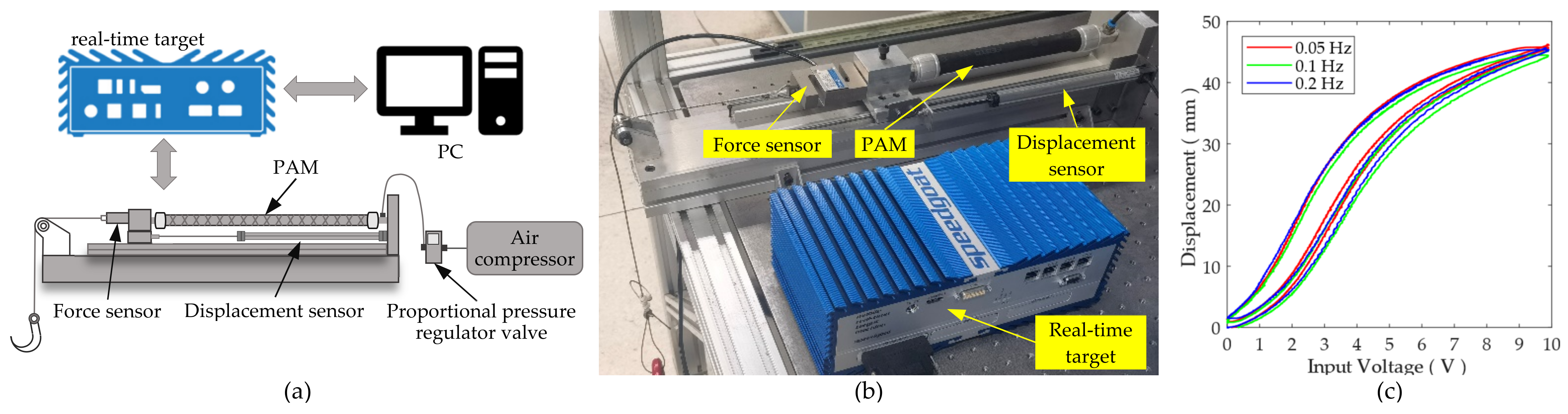
In this paper, a testbench is developed to simultaneously record the control input, the output displacement, and the output force of the PAM to facilitate the 3D hysteresis modeling of PAMs. As shown in Figure 1, the PAM is installed on a linear guiding rail system with one end clamped and the other end sliding along the rail. The inner pressure of the PAM is controlled by a proportional pressure regulator valve (model VPPM-6L-1-G18-0L6H from Festo) with the help of an air compressor. The displacement of the PAM is measured using a displacement sensor (Model 102322/A from novotechnik). A force sensor (Model H3-C3-200 kg-3B from ZEMIC) is used to measure the external force applied on the PAM or the payload of the system. The data acquisition is implemented in the environment of a real-time target machine (Model Mobile from Speedgoat). The overall system runs at a sampling rate of 1 kHz. Different PAMs can be installed on the testbench for the characterization and testing.
2.2. The Input-Displacement Hysteresis of the PAM
As previously mentioned, there is an obvious hysteresis nonlinearity between the input and the displacement of the PAM. In this paper, the input voltage applied to the pressure regulator valve is adopted as the input of the overall system. First, the input-displacement hysteresis is investigated by removing the external load from the PAM. In this case, the output force can be treated as 0. The following sinusoidal signal is adopted as the input:
where u represents the input, f is the frequency of the signal, and A and δ are the maximum allowable voltage and the dead zone of the pressure regulator valve, respectively.
For the selected pressure regular valve, A = 10 and δ = 0.1. In human–machine interactions, the PAM generally works at a relatively slow speed. As a result, in the preliminary tests, the frequency of the signal is set to f = 0.05, 0.1, and 0.2 Hz. The displacements of the PAM are measured, and the input–displacement hysteresis loops are shown in Figure 1c. It can be easily found that the PAM’s hysteresis loop is not symmetric about its loop center. As the frequencies are low in Figure 1c, the rate dependence of the PAM’s hysteresis is observable but not very obvious.
2.3. The Couplings between the Output Force and Displacement
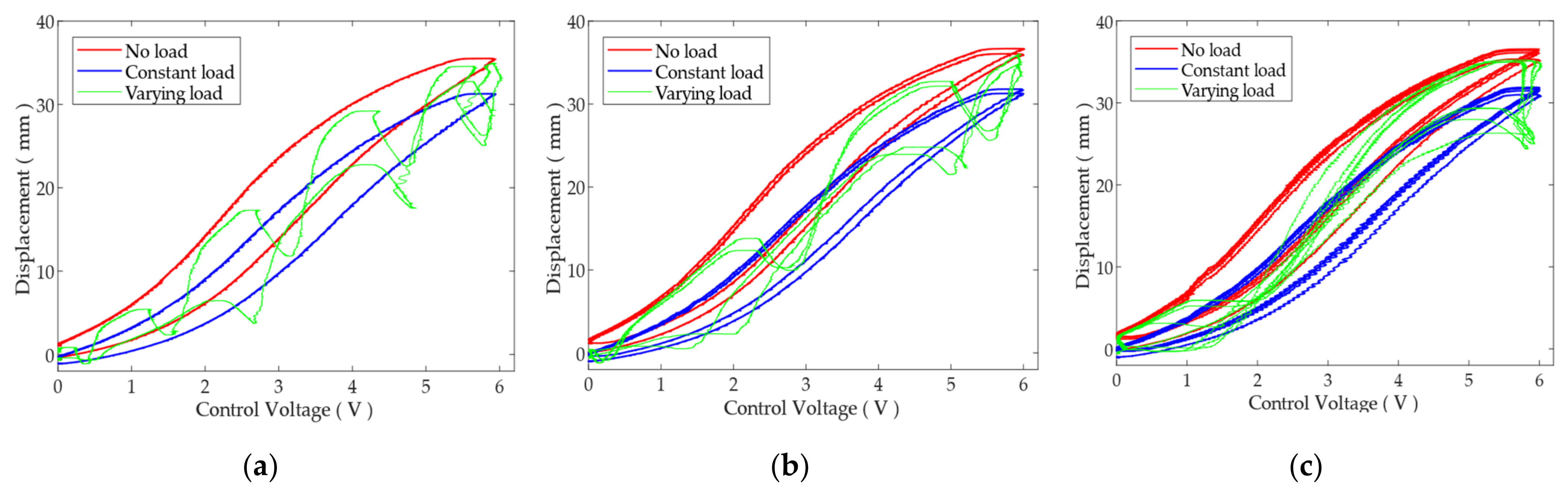
As the PAM is a flexible actuator, its displacement and force are coupled. The variation in the external load or disturbances will significantly affect the PAM’s displacement [8]. In order to intuitively demonstrate the couplings between the output force and displacement, external forces are added to the free end of the PAM when the PAM moves back and forth. First, all the load is removed from the PAM. In this case, the measured hysteresis all comes from the PAM itself. Secondly, a constant load (~91 N) is added to the hook. Finally, the hook is pulled by hand to provide a varying load. Figure 2 shows the PAM’s behaviors in the above scenarios at different frequencies.
It can be found from Figure 2 that the external load will significantly affect the behavior of the PAM. For the constant load, the stroke of the PAM will decrease, i.e., the hysteresis loop of the PAM will be squeezed along the Y axis. It is noted that the shape of the hysteresis loop is basically unchanged. However, when the external load is varying during the process, there exist several regional distortions on the measured hysteresis loops. As a result, it will be very difficult to model such a distorted hysteresis loop using 2D hysteresis models.
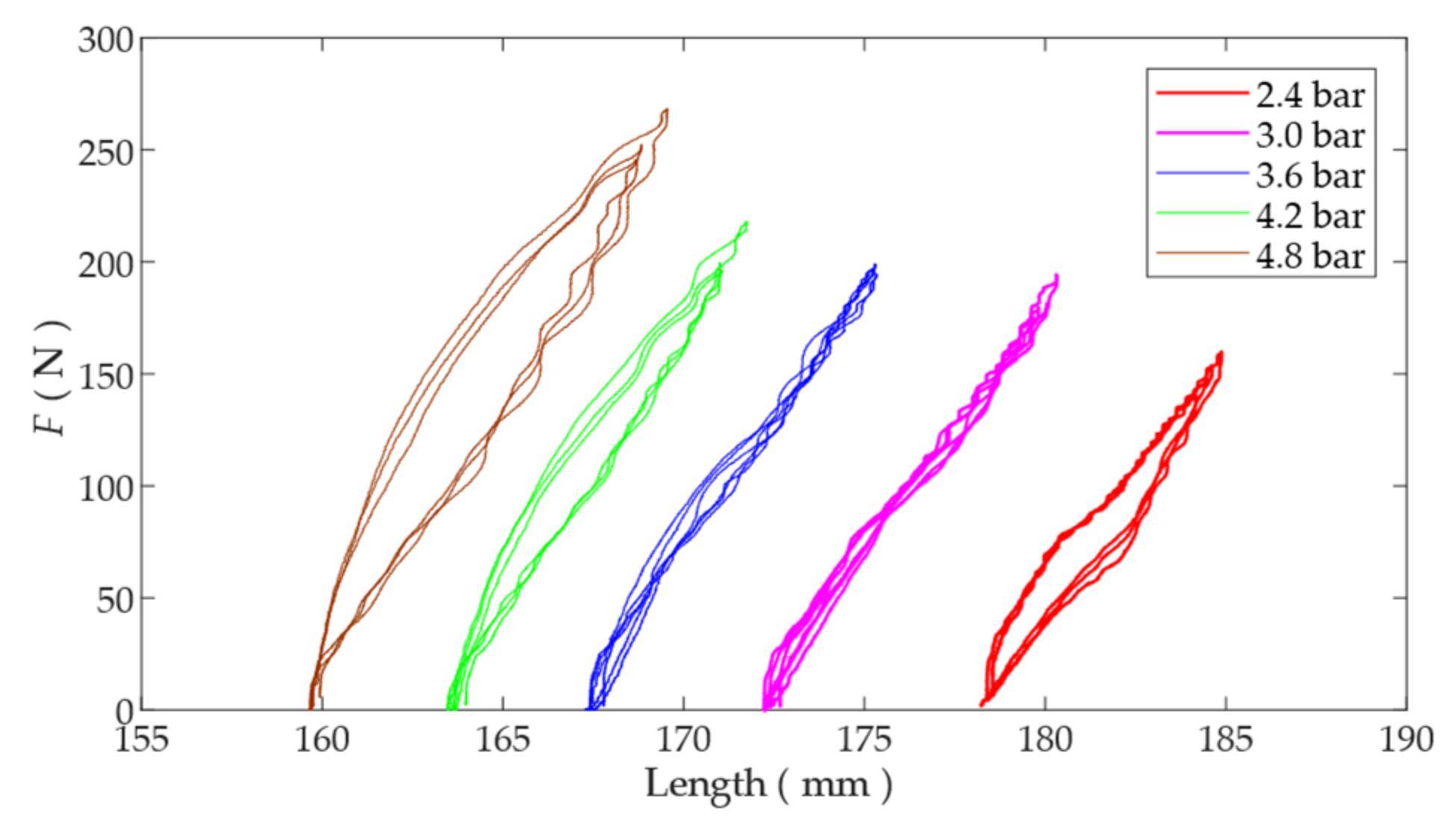
The couplings between the output force and displacement are also experimentally investigated. In this case, the inner pressure is kept constant at different levels, and the relationship between the external load and the displacement of the PAM is measured. The experimental results are plotted in Figure 3. It is observed that hysteresis loops can also be found between the output force and displacement of the PAM.
Based on the above results, it is clear that there exist a strong hysteresis and couplings among the input, the output force, and the displacement of the PAM. The 3D hysteresis model is required to obtain an accurate model of such a complex system.
3. MPI-NARMAX Hysteresis Model
In this paper, a 3D hysteresis model, namely the MPI-NARMAX model, is proposed for modeling the complex relationship among the input-displacement-force of the PAM. The schematic diagram of the model is illustrated in Figure 4, where the current input voltage, the current external force, and the historical output displacement are adopted as inputs. The proposed model can be divided into a hysteresis modeling unit and a coupling unit. In the hysteresis modeling unit, the MPI model is used to characterize the hysteresis between the input voltage and the output displacement of the PAM when no external load is applied. Subsequently, in the coupling unit, the NARMAX model is used to model the couplings between the output force and displacement of the PAM. Compared with the 2D hysteresis models, the proposed 3D hysteresis model is developed to predict the PAM’s behavior even when confronted with varying external loads.
3.1. The MPI Model
The classical PI model is a widely used hysteresis model consisting of a set of weighted backlash operators. The backlash operator is defined as follows:
where u represents the input of the operator, hi represents the output of the ith backlash operator, ri is the threshold, and T represents the sampling period. Then, the classical PI model can be obtained by the weighted summation of a series of backlash operators:
where n is defined as the order of the model, ωi is the weight for hi, and b(t) represents the output of the classical PI model.
The hysteresis of PAM is rate-dependent, whereas the classical PI model is static. In order to account for the rate dependence, the weights of backlash operators can be linearly adjusted according to the input rate, which can be described as follows:
where ki is the slope and di is the intercept.
From Figure 1c, it can be observed that the hysteresis loop of the PAM is asymmetric. However, the classical PI model is a symmetric model, making it difficult to describe the asymmetry of the PAM’s hysteresis well. Based on our previous work, a polynomial operator can capture well the asymmetry and improve the modeling accuracy [13]. Therefore, the following polynomial operator is integrated to form the MPI model:
where f(t) represents the polynomial output, ai represents the polynomial coefficient, and bi(t) represents the ith power of the output of the classical PI model in (3).
3.2. NARMAX Model Based on RFNN
The NARMAX model can be used to deal with the identification problem of nonlinear systems [19]. A nonlinear system can be described as:
where y(t) and x(t) represent the output and input of the NARMAX model, respectively, ny and nx represent maximum time lags associated with y(t) and x(t), respectively, and g(•) represents the nonlinear relationship between the outputs and inputs.
For the hysteretic system in this paper, the NARMAX model can be described as:
where ŷ(t) represents the predictive output of the system, f(t) represents the output of the MPI model, F(t) is the output force of the PAM, and na, nb, and nc represent the maximum orders in ŷ(t), f(t), and F(t), respectively.
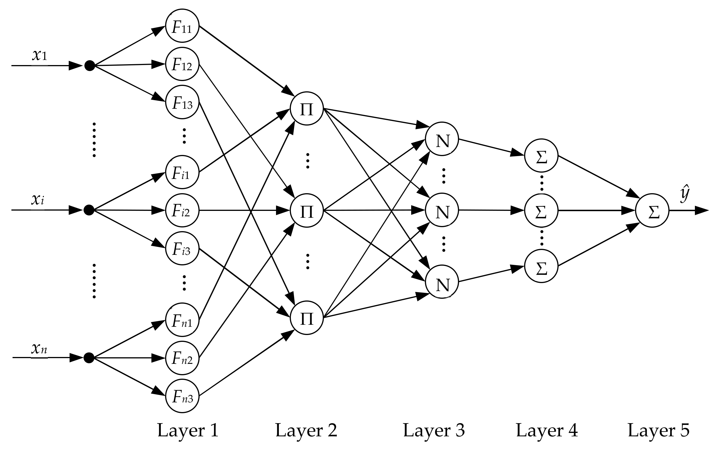
Based on previous research [20,21], g(•), the nonlinear mapping relationship between ŷ(t), f(t), and F(t), can be identified by neural networks. Therefore, the recurrent fuzzy neural network (RFNN) is selected in this paper to identify the NARMAX model. Generalized from the fuzzy neural network (FNN), the RFNN was shown to possess the same advantages over recurrent neural networks and extend the application domain of the FNN to temporal problems [22]. In this paper, the structure of the RFNN is shown in Figure 5. For the convenience of subsequent expression, N is defined as:
There are 5 layers in the RFNN. The first layer includes 3N neurons, i.e., 3 fuzzy operators for each input. It realizes time recursion and the fuzzification process. The output of each node can be described as:
where xi represents the ith input element, j represents the ordinal number of the fuzzy operator, mij and σij are parameters of the Gaussian membership function, and θij is the parameter of time recursion.
The second layer, which contains 3N neurons, combines the outputs of the first layer to achieve the nonlinearity of the output:
The third layer, which has the same number of neurons as the second layer, normalizes the output of each node in the previous layer:
The fourth layer multiplies the output of the previous layer as a weight on the input:
Finally, the fifth layer sums the outputs of the fourth layer:
4. Experimental Results
4.1. Parameter Identification of MPI Model
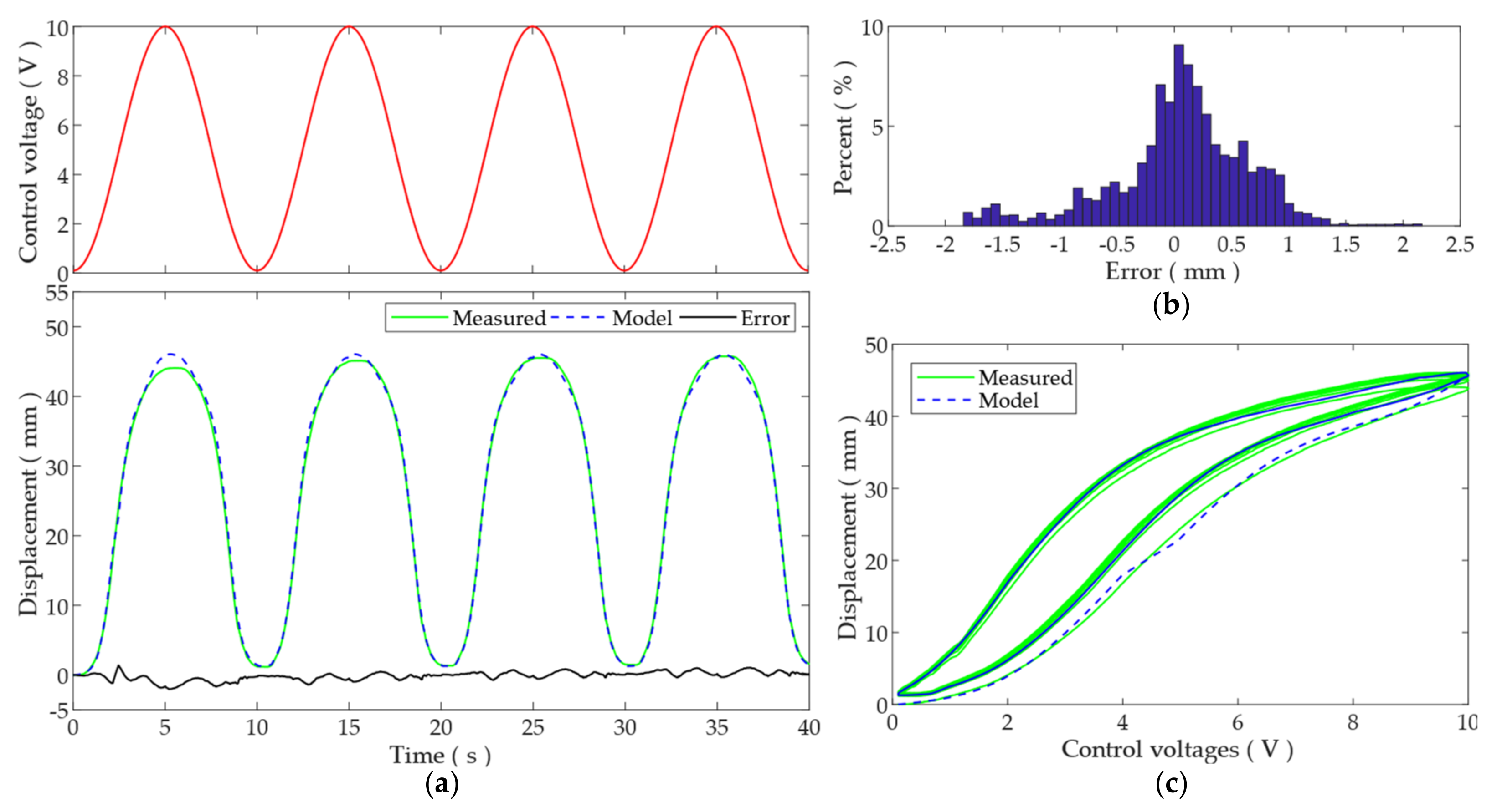
In the MPI model, the parameters that need to be identified include ri, ki, di, and ai. The least squares method is used to identify the MPI model from the experimental results of the 0.1 Hz sinusoidal excitation without load. The identified parameters are given in Table 1. The measured displacement and model output are shown in Figure 6. It can be observed that great agreement between the measurement and the model output has been achieved, as shown in Figure 6a,c. In order to quantify the modeling accuracy, the mean absolute error (MAE) and root-mean-square error (RSME) are calculated to be 0.4538 mm and 0.6120 mm, respectively.
The statistics of the modeling error are shown in Figure 6b. It can be observed that the modeling errors center around 0 and lie mainly within the range of ±1 mm. As a result, the MPI model can well predict the PAM’s displacement when no load is added to the system. However, the influence of the external load is not considered in MPI model. Typically, if a constant load is added to the hook, the same modeling and identification process has to be repeated to obtain another MPI model. This is straightforward and thus is not be presented herein, to guarantee the conciseness of the paper.
4.2. Training of RFNN
In order to capture the influence of the time-varying load on the PAM’s displacement, different external loads are applied on the hook when the PAM is moving. The output force and displacement of PAM are measured during the process. The output of the MPI model, the output force, and the displacement of the PAM are used as the training data for the RFNN.
In the training of the RFNN, the standard particle swarm optimization (PSO) method is used to identify the parameters of the RFNN. PSO is initialized by a group of particles, and the optimal solution is found in the subsequent iterative update. The updating rule of particles can be expressed by the following formulas:
where qi(t) and vi(t) represent the current position and velocity of the particle, respectively, wv is the inertial weight, c1 and c2 represent the learning constants, rand() represents the random number, and pbest and gbest represent the best position for the individual particle and all particles, respectively.
The linear decreasing weight is used to update the inertial weight wv. The updating rule of wv can be expressed by the following formula:
where m represents the current iteration number. In this paper, the learning constant c1 and c2 are set to be 2. wini and wend, which represent the initial and final value of wv, respectively, are set to 0.9 and 0.4.
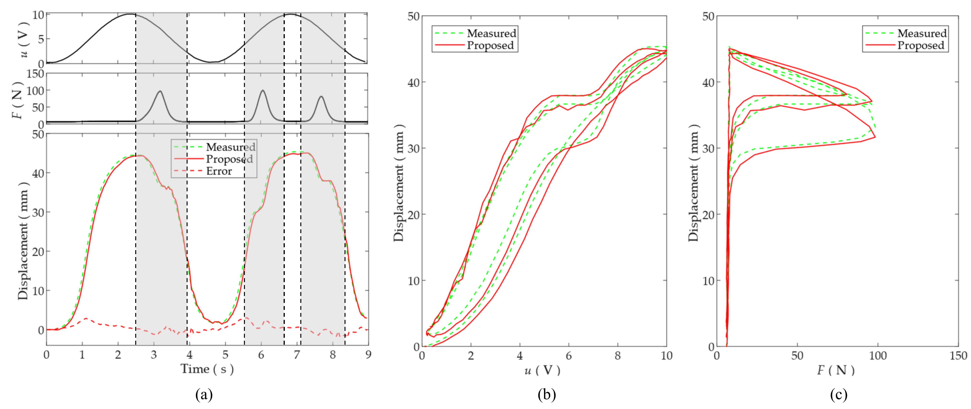
The overall 3D hysteresis model can be obtained after training the RFNN and cascading it to the MPI model. The experimental results of the training set are shown in Figure 7. The external load with a peak of approximately 100 N is applied and removed from the hook three times. The shaded areas in Figure 7a indicate the durations of the external load. In this manner, the PAM’s behaviors with and without external load can be captured in one measurement. It can be found from Figure 7 that when there is no external load, the MPI-NARMAX model can follow the displacement of the PAM well. When there is external load on the PAM, the MPI-NARMAX model can still predict the output displacement of PAM well. There is no obvious change in the magnitude of the modeling error for the PAM with and without external loads. The MAE and RMSE are calculated to be 0.8730 mm and 1.0913 mm, respectively. Due to the influence of the external load, the input–displacement hysteresis loops are distorted, as shown in Figure 7b. This will be difficult to model using conventional 2D hysteresis models. The couplings between the force and displacement of the PAM are shown in Figure 7c. It can be observed that the proposed MPI-NARMAX successfully captures the influence of the external load and improves the prediction accuracy on the output displacement of the PAM. As shown in Figure 7b, the input–displacement relationship of the MPI-NARMAX model matches the measurement well.
4.3. The Results of MPI-NARMAX Model
4.3.1. Varying Load
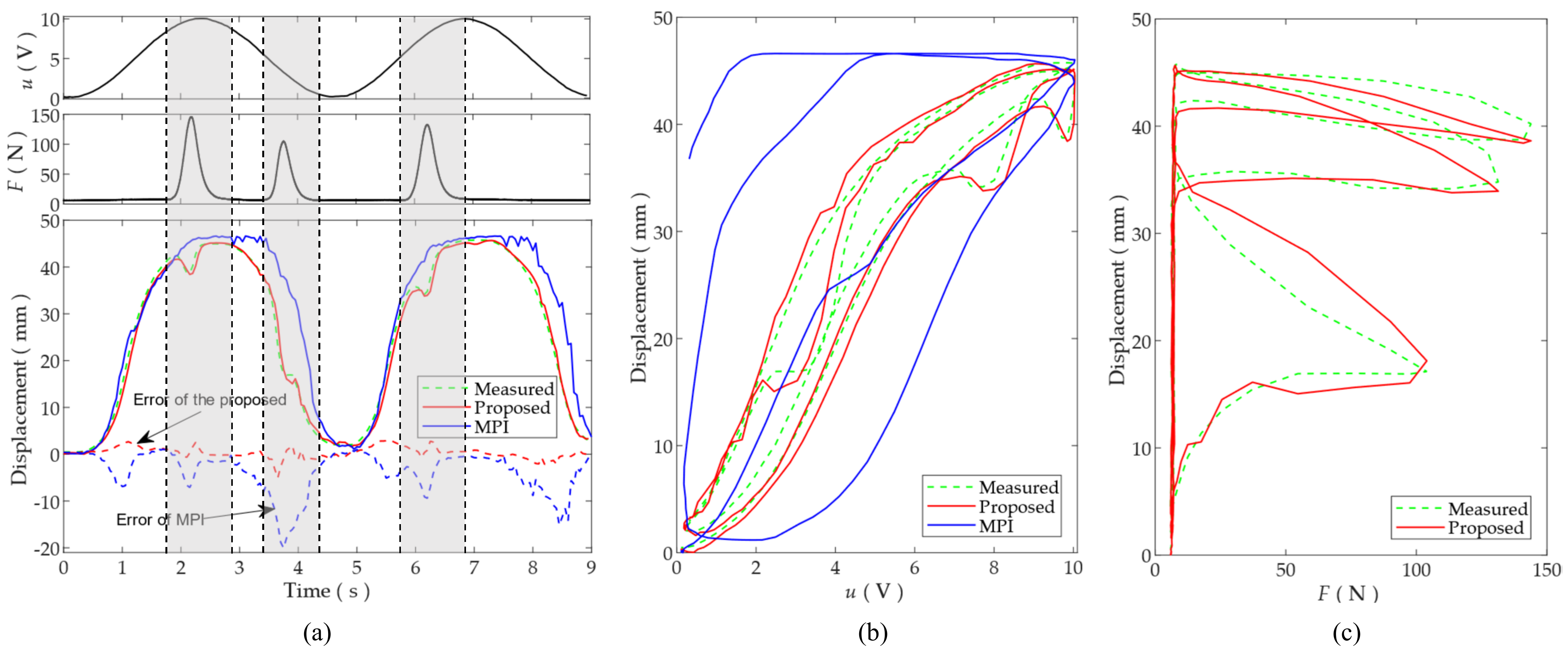
The effectiveness of the identified MPI-NARMAX model is verified on another testing dataset, where the PAM is confronted with stronger external forces. The experimental results of the testing set are shown in Figure 8.
Similar to the training set, the external load is applied and removed from the hook three times. However, the peak of the external load increases to approximately 150 N. For such a high and varying external force, the proposed model can still precisely predict the output displacement. The MAE and RSME are calculated to be 0.9304 mm and 1.2138 mm, respectively. The modeling error on the testing set is comparable to the modeling error on the training set. The input–displacement hysteresis loops and force–displacement couplings are shown in Figure 8b,c, respectively. Good agreements between the measurements and the model output can be found. This demonstrates that the complex relationship among the input, the output displacement, and the output force of the PAM can be captured well in the proposed 3D hysteresis model.
In order to compare the performance of the proposed model, the performance of the MPI model identified in Section 4.1 is also provided in Figure 8. As this standalone MPI model is identified without any external load, the influence of the external load is totally ignored in this MPI model. As a result, there exist obvious discrepancies between the MPI’s output and the measurement. The modeling accuracy of the standalone MPI model is poor. The MAE and RMSE of the MPI model are calculated to be 3.8926 mm and 4.4845 mm, respectively. This demonstrates that the conventional 2D hysteresis models cannot capture the couplings between the output force and displacement of the PAM. The modeling accuracy of the 2D models are poor when confronted with strong and varying external loads.
4.3.2. Cross-Checking with Different Load Statuses
In applications, the influence of the external load can also be modeled by applying different payloads to the PAM and identifying the parameters of the standalone MPI model for each payload. As a result, instead of a single model, multiple MPI models are obtained using this method. In order to compare the performance of the proposed MPI-NARMAX model with these models, the PAM’s behaviors in the following load statuses are measured:
- Status 1:
- 0.1 Hz sinusoidal signal actuation without load.
- Status 2:
- 0.2 Hz sinusoidal actuation with a constant load of 10.04 kg.
- Status 3:
- 0.2 Hz sinusoidal actuation with a constant load of 21.75 kg.
- Status 4:
- 0.22 Hz sinusoidal actuation with varying load, as investigated in Figure 8.
In status 4, it is very difficult to use a standalone MPI model to fit the measurement, as the measured hysteresis loops contain several regional distortions. As a result, three MPI models are individually identified at status 1, 2, and 3, which are denoted as MPI-1, MPI-2, and MPI-3, respectively.
The identified MPI models, together with the proposed MPI-NARMAX model, are cross-checked using the other measurements. The MAE and RMSE of these models with different load statuses are calculated and listed in Table 2 and Table 3, respectively.
For standalone MPI models, it is observed that a low modeling error is achieved in identification, as marked in bold. As a result, if the load status remains, a high modeling accuracy is expected. However, if the load status changes, the modeling error increases obviously. For the varying load in status 4, the modeling accuracy of all the standalone MPI models is poor.
On the contrary, the modeling accuracy of the proposed MPI-NARMAX model is consistent, regardless of the change in the load status. For constant loads, the modeling error of the proposed MPI-NARMAX model is comparable to the standalone MPI models individually identified. For the varying load in status 4, the modeling accuracy of the proposed model is the best among the models.
The above experimental results also demonstrate that the proposed MPI-NARMAX model is effective for both constant and varying external loads. It is superior to the standalone MPI models individually identified at different constant loads as it can adapt to different load statuses after only one training, and the parameter identification process does not need to be repeated when the external load changes.
5. Conclusions
For PAMs, there exists strong hysteresis between the input and outputs. In addition, the coupling between the output displacement and output force is obvious. These make the precise modeling of the PAM’s behavior very difficult, especially when varying external load or disturbances occur. This paper proposes a displacement and force hybrid 3D hysteresis model, where the MPI model and RFNN-based NARMAX model are integrated. The MPI model is constructed by cascading a polynomial saturation operator to the classical PI model to account for the asymmetry of the PAM’s hysteresis. The RFNN-based NARMAX model is used to capture the couplings between the output force and displacement of the PAM. Similar research work can be found in Zhang’s paper [17], where the weight of the constant payload is included in the training data, making the model capable of predicting the behavior of the PAM with different but constant loads. In this paper, with the help of a force sensor, the dynamic variation in the external load can be measured and included as one input to the model. This makes the proposed MPI-NARMAX hysteresis model capable of predicting the PAM’s behavior regardless of the change in the external load.
The proposed MPI-NARMAX model only needs to be identified and trained once. The experimental results of the PAM with constant and varying external loads verify that the proposed MPI-NARMAX hysteresis model successfully captures the complex hysteresis and couplings among the input, the output displacement, and the output force of the PAM. It is capable of precisely predicting the output of the PAM when confronted with constant and varying external loads. The modeling accuracy is robust against the variation in the external load. The effectiveness and applicability of the proposed MPI-NARMAX model are verified.
Author Contributions
Y.Q.: Conceptualization, methodology, resources, writing—review and editing, supervision, project administration, funding acquisition; Y.X.: conceptualization, software, validation, formal analysis, investigation, data curation, writing—original draft preparation; C.S.: conceptualization, software, data curation; J.H.: methodology, resources, project administration, funding acquisition. All authors have read and agreed to the published version of the manuscript.
Funding
This work was supported by the National Natural Science Foundation of China (Nos. 61873133, U1913208, and 61873135).
Institutional Review Board Statement
Not applicable.
Informed Consent Statement
Not applicable.
Data Availability Statement
Not applicable.
Conflicts of Interest
The authors declare no conflict of interest.
References
- Tondu, B. Modelling of the McKibben artificial muscle: A review. J. Intell. Mater. Syst. Struct. 2012, 23, 225–253. [Google Scholar] [CrossRef]
- Vo-Minh, T.; Tjahjowidodo, T.; Ramon, H.; Van Brussel, H. A new approach to modeling hysteresis in a pneumatic artificial muscle using the Maxwell-slip model. IEEE/ASME Trans. Mechatron. 2011, 16, 177–186. [Google Scholar] [CrossRef]
- Tsagarakis, N.G.; Caldwell, D.G. Development and control of a ‘soft-actuated’ exoskeleton for use in physiotherapy and training. Auton. Robot. 2003, 15, 21–33. [Google Scholar] [CrossRef]
- Liu, Y.; Zang, X.; Lin, Z.; Li, W.; Zhao, J. Position control of a bio-inspired semi-active joint with direct inverse hysteresis modeling and compensation. Adv. Mech. Eng. 2016, 8, 168781401667722. [Google Scholar] [CrossRef] [Green Version]
- Meng, W.; Liu, Q.; Zhang, M.; Ai, Q.; Xie, S.Q. Compliance adaptation of an intrinsically soft ankle rehabilitation robot driven by pneumatic muscles. In Proceedings of the 2017 IEEE/ASME International Conference on Advanced Intelligent Mechatronics, Munich, Germany, 3–7 July 2017; pp. 82–87. [Google Scholar]
- Yang, H.; Xiang, C.; Hao, L.; Zhao, L.; Xue, B. Research on PSA-MFAC for a novel bionic elbow joint system actuated by pneumatic artificial muscles. J. Mech. Sci. Technol. 2017, 31, 3519–3529. [Google Scholar] [CrossRef]
- Minh, T.V.; Kamers, B.; Ramon, H.; Van Brussel, H. Modeling and control of a pneumatic artificial muscle manipulator joint—Part I: Modeling of a pneumatic artificial muscle manipulator joint with accounting for creep effect. Mechatronics 2012, 22, 923–933. [Google Scholar] [CrossRef]
- Minh, T.V.; Tjahjowidodo, T.; Ramon, H.; Van Brussel, H. Cascade position control of a single pneumatic artificial muscle-mass system with hysteresis compensation. Mechatronics 2010, 20, 402–414. [Google Scholar] [CrossRef]
- Sofla, M.S.; Sadigh, M.J.; Zareinejad, M. Design and dynamic modeling of a continuum and compliant manipulator with large workspace. Mech. Mach. Theory 2021, 164, 104413. [Google Scholar] [CrossRef]
- Shakiba, S.; Ourak, M.; Poorten, E.V.; Ayati, M.; Yousefi-Koma, A. Modeling and compensation of asymmetric rate-dependent hysteresis of a miniature pneumatic artificial muscle-based catheter. Mech. Syst. Signal Processing 2021, 154, 107532. [Google Scholar] [CrossRef]
- Liang, D.; Sun, N.; Wu, Y.; Chen, Y.; Fang, Y.; Liu, L. Energy-based Motion Control for Pneumatic Artificial Muscle-Actuated Robots With Experiments. IEEE Trans. Ind. Electron. 2021, 2021, 3095788. [Google Scholar] [CrossRef]
- Qin, Y.; Xu, Y.; Han, J. Hysteresis Compensation of Pneumatic Artificial Muscle ActuatedAssistive Robot for the Elbow Joint. Jiqiren/Robot 2021, 43, 453–462. (In Chinese) [Google Scholar] [CrossRef]
- Qin, Y.; Tian, Y.; Zhang, D.; Shirinzadeh, B.; Fatikow, S. A novel direct inverse modeling approach for hysteresis compensation of piezoelectric actuator in feedforward applications. IEEE/ASME Trans. Mechatron. 2013, 18, 981–989. [Google Scholar] [CrossRef]
- Mohareb, S.A.; Alsharkawi, A.; Zgoul, M. Hysteresis modeling of a pam system using anfis. Actuators 2021, 10, 280. [Google Scholar] [CrossRef]
- Kogiso, K.; Sawano, K.; Itto, T.; Sugimoto, K. Identification procedure for McKibben pneumatic artificial muscle systems. In Proceedings of the IEEE International Conference on Intelligent Robots and Systems, Vilamoura-Algarve, Portugal, 7–12 October 2012; pp. 3714–3721. [Google Scholar]
- Sofla, M.S.; Sadigh, M.J.; Zareinejad, M. Precise dynamic modeling of pneumatic muscle actuators with modified Bouw-Wen hysteresis model. Proc. Inst. Mech. Eng. Part E J. Process Mech. Eng. 2021, 235, 1449–1457. [Google Scholar] [CrossRef]
- Zhang, Y.; Liu, H.; Ma, T.; Hao, L.; Li, Z. A comprehensive dynamic model for pneumatic artificial muscles considering different input frequencies and mechanical loads. Mech. Syst. Signal Processing 2021, 148, 107133. [Google Scholar] [CrossRef]
- Konda, R.; Zhang, J. Hysteresis with lonely stroke in artificial muscles: Characterization, modeling, and inverse compensation. Mech. Syst. Signal Processing 2022, 164, 108240. [Google Scholar] [CrossRef]
- Leontaritis, I.J.; Billings, S.A. Input-output parametric models for non-linear systems Part I: Deterministic non-linear systems. Int. J. Control 1985, 41, 303–328. [Google Scholar] [CrossRef]
- Gu, Y.; Li, B.; Meng, Q. Hybrid interpretable predictive machine learning model for air pollution prediction. Neurocomputing 2022, 468, 123–136. [Google Scholar] [CrossRef]
- Araluce, J.; Bergasa, L.M.; Ocaña, M.; López-Guillén, E.; Revenga, P.A.; Felipe Arango, J.; Pérez, O. Gaze focalization system for driving applications using openface 2.0 toolkit with NARMAX algorithm in accidental scenarios. Sensors 2021, 21, 6262. [Google Scholar] [CrossRef]
- Lee, C.H.; Teng, C.C. Identification and control of dynamic systems using recurrent fuzzy neural networks. IEEE Trans. Fuzzy Syst. 2000, 8, 349–366. [Google Scholar] [CrossRef]
Figure 1.
The developed testbench: (a) the schematic diagram of the overall system, (b) the photo of the testbench, and (c) the hysteresis loops of the PAM at different frequencies.
Figure 1.
The developed testbench: (a) the schematic diagram of the overall system, (b) the photo of the testbench, and (c) the hysteresis loops of the PAM at different frequencies.

Figure 2.
The influences of the load and external disturbances on the PAM’s displacement: (a) 0.05 Hz, (b) 0.1 Hz, and (c) 0.2 Hz.
Figure 2.
The influences of the load and external disturbances on the PAM’s displacement: (a) 0.05 Hz, (b) 0.1 Hz, and (c) 0.2 Hz.

Figure 3.
The force–displacement couplings of the PAM.

Figure 4.
The schematic diagram of the proposed MPI-NARMAX hysteresis model.

Figure 5.
Structure of the RFNN.

Figure 6.
Identification of the MPI model: (a) time plot, (b) error histogram, and (c) hysteresis plot.
Figure 6.
Identification of the MPI model: (a) time plot, (b) error histogram, and (c) hysteresis plot.

Figure 7.
Training of the RFNN: (a) time plots of the input and outputs with shaded areas indicating the durations of the external load, (b) the input–displacement hysteresis, and (c) the force–displacement couplings.
Figure 7.
Training of the RFNN: (a) time plots of the input and outputs with shaded areas indicating the durations of the external load, (b) the input–displacement hysteresis, and (c) the force–displacement couplings.

Figure 8.
Verification of the proposed MPI-NARMAX model: (a) time plots of the input and outputs with shaded areas indicating the durations of the external load, (b) the input–displacement hysteresis, and (c) the force–displacement couplings.
Figure 8.
Verification of the proposed MPI-NARMAX model: (a) time plots of the input and outputs with shaded areas indicating the durations of the external load, (b) the input–displacement hysteresis, and (c) the force–displacement couplings.


Table 1.
Identification result of the parameters.
| i | 1 | 2 | 3 | 4 | 5 | 6 | 7 | 8 | 9 | 10 |
|---|---|---|---|---|---|---|---|---|---|---|
| ri | 0 | 0.0101 | 0.0296 | 0.2596 | 0.4318 | 0.8309 | 1.6003 | 1.9544 | 3.9537 | 4.95 |
| ki | 3.5838 | −3.8779 | 0.3084 | 0.1117 | −0.0887 | −0.0033 | −0.0116 | −0.0208 | −0.0429 | 0.0315 |
| di | −0.3435 | 0.643 | −0.1711 | 0.1878 | −0.0425 | 0.0359 | 0.046 | 0.0461 | −0.0298 | 0.0698 |
| ai | −8.97e-04 | 0 | 0.0411 | 0 | −0.6712 | 0 | 4.4945 | 0 | 2.3917 | 0 |
Table 2.
The MAE with different load statuses.
| Status 1 | Status 2 | Status 3 | Status 4 | |
|---|---|---|---|---|
| MPI-1 | 0.5675 | 6.8589 | 10.0609 | 3.8926 |
| MPI-2 | 4.6434 | 0.1716 | 3.2333 | 3.6108 |
| MPI-3 | 7.8112 | 3.2266 | 0.1628 | 6.7443 |
| MPI-NARMAX | 0.3094 | 0.2887 | 0.3676 | 0.9304 |
Table 3.
The RMSE with different load statuses.
| Status 1 | Status 2 | Status 3 | Status 4 | |
|---|---|---|---|---|
| MPI-1 | 0.6577 | 5.4060 | 6.5387 | 4.4845 |
| MPI-2 | 2.9424 | 0.2348 | 1.9331 | 2.3808 |
| MPI-3 | 4.5439 | 1.9357 | 0.2146 | 3.8913 |
| MPI-NARMAX | 0.3997 | 0.3887 | 0.4668 | 1.2138 |
Publisher’s Note: MDPI stays neutral with regard to jurisdictional claims in published maps and institutional affiliations. |
© 2022 by the authors. Licensee MDPI, Basel, Switzerland. This article is an open access article distributed under the terms and conditions of the Creative Commons Attribution (CC BY) license (https://creativecommons.org/licenses/by/4.0/).
Share and Cite
MDPI and ACS Style
Qin, Y.; Xu, Y.; Shen, C.; Han, J. High-Precision Displacement and Force Hybrid Modeling of Pneumatic Artificial Muscle Using 3D PI-NARMAX Model. Actuators 2022, 11, 51. https://doi.org/10.3390/act11020051
AMA Style
Qin Y, Xu Y, Shen C, Han J. High-Precision Displacement and Force Hybrid Modeling of Pneumatic Artificial Muscle Using 3D PI-NARMAX Model. Actuators. 2022; 11(2):51. https://doi.org/10.3390/act11020051
Chicago/Turabian StyleQin, Yanding, Yuankai Xu, Chenyu Shen, and Jianda Han. 2022. "High-Precision Displacement and Force Hybrid Modeling of Pneumatic Artificial Muscle Using 3D PI-NARMAX Model" Actuators 11, no. 2: 51. https://doi.org/10.3390/act11020051
Note that from the first issue of 2016, this journal uses article numbers instead of page numbers. See further details here.