
Fourier Neural Operator for Fluid Flow in Small-Shape 2D Simulated Porous Media Dataset


1
Department of Computer Science, University of Liverpool, Liverpool L69 7ZX, UK
2
Department of Applied Mathematics, Xi’an Jiaotong-Liverpool University, Suzhou 215123, China
3
DWA Energy Limited, Lincoln LN5 9JP, UK
*
Authors to whom correspondence should be addressed.
Algorithms 2023, 16(1), 24; https://doi.org/10.3390/a16010024
Submission received: 5 December 2022
/
Revised: 25 December 2022
/
Accepted: 26 December 2022
/
Published: 1 January 2023
(This article belongs to the Special Issue Deep Learning Architecture and Applications)
Abstract
:Machine Learning (ML) and/or Deep Learning (DL) methods can be used to predict fluid flow in porous media, as a suitable replacement for classical numerical approaches. Such data-driven approaches attempt to learn mappings between finite-dimensional Euclidean spaces. A novel neural framework, named Fourier Neural Operator (FNO), has been recently developed to act on infinite-dimensional spaces. A high proportion of the research available on the FNO has focused on problems with large-shape data. Furthermore, most published studies apply the FNO method to existing datasets. This paper applies and evaluates FNO to predict pressure distribution over a small, specified shape-data problem using 1700 Finite Element Method (FEM) generated samples, from heterogeneous permeability fields as the input. Considering FEM-calculated outputs as the true values, the configured FNO model provides superior prediction performance to that of a Convolutional Neural Network (CNN) in terms of statistical error assessment based on the coefficient of determination (R) and Mean Squared Error (MSE). Sensitivity analysis considering a range of FNO configurations reveals that the most accurate model is obtained using and . Graphically, the FNO model precisely follows the observed trend in each porous medium evaluated. There is potential to further improve the FNO’s performance by including physics constraints in its network configuration.
1. Introduction
A wide range of phenomena/processes in science and engineering are described via measurable/estimable quantities that rely on independent variables. As an example, in subsurface fluid flow, pressure and temperature are typically measured based on the time and location variables. Given the available fundamental laws, it is feasible to determine the relationships among the rates of change of these physical quantities. The mathematical correlations typically used to do this are Ordinary and/or Partial Differential Equations (ODEs/PDEs). In ODEs, the derivatives of the dependent variable(s) are taken with respect to only one independent variable. On the other hand, partial derivatives are required in PDEs when there are two or more independent variables involved.
Theories, methods, and tools available in scientific computing (also called computational science) make it possible to solve mathematical models of physical phenomena described in terms of ODEs and/or PDEs [1]. The theories and methods are together called numerical analysis/numerical mathematics, and tools refer to computer systems on which codes are run. The more complex the mathematical models, the more advanced the computational hardware requirements are to solve them. There are various numerical methods available that can provide approximate solutions to such problems. These include the finite difference method [2], Finite Element Method (FEM) [3], finite volume method [4], spectral method [5], and meshless method [6]. Such methods are usually time-consuming to apply.
One way to mitigate the problem of the high computational cost in numerical calculations required to determine complex systems is to apply Machine Learning (ML) and/or Deep Learning (DL) techniques. Machine learning methods such as Neural Network (NN), adaptive-neuro-fuzzy-inference system, support-vector machine, and decision tree are widely employed to find and predict relevant patterns within datasets. Machine learning is now used to great advantage in various fields [7,8,9,10]. Deep learning methods represent more complex extensions of existing ML methods, particularly neural networks, and have demonstrated improved performance, particularly when applied to large datasets [11,12,13,14,15]. There are various DL algorithms, including Convolutional Neural Network (CNN), deep auto-encoder, deep-belief network, recurrent neural network, and generative adversarial network. There are some differences between ML and DL. For instance, manual feature engineering tends to be performed with ML algorithms, sometimes requiring domain knowledge about a given problem. To make the point clear, consider ’filling missing values’. A dataset can include missing values due to the difficulty of collecting complete data. Missing values can be manually filled in based on expert knowledge, which is sometimes a tedious process. However, with DL algorithms this is more often not required, being performed automatically.
Classical neural networks concentrate on learning mappings between finite-dimensional spaces. This makes such networks, when configured, confined to a particular discretization (i.e., they are mesh-dependent). Mesh-independent networks have been developed to reduce such constraints. In this regard, the Fourier Neural Operator (FNO) has recently been proposed to learn a continuous function via parameterizing the model in its function space [16]. This makes it possible for FNO to be trained on one mesh and subsequently evaluated on another. Unlike standard feed-forward networks that use activation functions (e.g., sigmoid, tanh, relu), training an FNO model using the Fourier transform to find optimum weights and biases is performed by employing sines and cosines as activation functions [17,18,19].
The Fourier neural operator has demonstrated its capabilities in solving parametric PDEs. Different models were developed to solve the Navier–Stokes equation for a viscous, incompressible fluid in vorticity form on the unit torus [16]. The viscosity was set to 0.001, 0.0001, and 0.00001. The resolution was for both training and testing. Based on the results, the FNO-3D had the best performance in the case of available sufficient data. When the amount of data was not sufficient, the FNO-2D achieved the lowest error.
An improved FNO-based DL model, U-FNO, was developed to solve a CO2-water multiphase flow problem over a wide range of rock–fluid properties, such as permeability, anisotropy, and flow rate [20]. The predictions generated for gas saturation and pressure buildup confirmed the superiority of the U-FNO model compared to FNO and CNN models applied to the same dataset. Additionally, U-FNO requires few training data to match the prediction accuracy of CNN.
As a substitute for physics-based solvers, an FNO framework was employed to learn/map certain mechanical responses of 2D composites [21]. The FNO models, trained with few data, were able to predict high-resolution stress/strain tensor fields for geometrically complex microstructures. Additionally, the models exhibited zero-shot generalization with high precision on random geometries previously unseen by the trained FNO model. Moreover, the trained FNO models were able to predict high-resolution stress/strain fields when presented with low-resolution inputs.
An FNO model has also been applied to a Large Eddy Simulation (LES) of a 3D turbulence system [22]. Filtered direct numerical simulation flow-field of isotropic turbulence recorded at different times comprised the training data. In the a posteriori test of LES, The FNO model outperformed dynamic Smagorinsky and dynamic mixed models to predict the velocity spectrum, probability density functions of vorticity and velocity increments, and the instantaneous flow structures.
In addition to solving parametric PDEs, FNO has been successfully applied to solve other problems. For example, FNO was used to classify images contained in the CIFAR-10 image database comprised of 60,000 distinct samples [23]. The input samples were color images of ten different classes. A total of 83% of the total dataset was used to train the FNO, and the remaining images were used to test the trained model. According to the different evaluation criteria, the FNO performed slightly better than ResNet20. However, the FNO model was computationally more costly.
As described, some research has been conducted applying FNO models to various existing datasets. However, much of that research addresses problems involving big-shape data (e.g., and ). Thus, there is a critical lack of analysis regarding the performance of FNO models on small-shape data. Consequently, the major contribution of this paper is to apply and evaluate an FNO model to predict pressure distribution in small-shape data (). Specifically, the study answers the following questions:
- (1)
- Can FNO models perform accurately on small-shape data problems in terms of the prediction error metrics?
- (2)
- How do mode and width affect the performance of FNO models?
- (3)
- Does downsampling have a positive or negative effect on FNO model performance when applied to small-shape data?
- (4)
- Can FNO models satisfy the pattern applicable to porous media problems?
- (5)
- How does the performance of FNO models compare to that of CNN?
A 30 × 30 uniform mesh problem from the domain of petroleum engineering is evaluated as a relevant topic with a suitable dataset to address the research questions identified. Continued constraints on the ability of the available energy supply to meet global energy demand make it important to improve our understanding of subsurface oil and gas reservoirs to improve production and resource recovery. The problem evaluated is designed to do that.
Comparing the FNO model performance with that of a CNN model applied to the same dataset is justified because CNNs are proven in their applications to 2D arrays and the mathematical basis underpinning convolutional-filter functionality is well established. Convolutional neural networks are also able to learn the spatial hierarchy of dataset characteristics on an unsupervised basis leading to good prediction performance based on relatively sparse feature selections.
The remaining sections of this article are arranged as follows. Section 2 describes the problem configuration and the dataset evaluated; Section 3 explains the configurations of the FNO and CNN models applied to the dataset and how their performances are optimized; Section 4 presents and compares the results generated by those two models; Section 5 discusses the limitations of the research; and Section 6 draws conclusions and makes recommendation for required future research.
2. Problem Setup with Governing Equations
The flow of fluids through porous media can be effectively described in terms of: (i) the Darcy (or momentum) law, (ii) mass conservation, (iii) energy drive, and (iv) case-specific rock–fluid correlations including compressibility and saturation equations, where more than one fluid is involved (e.g., gas, oil and/or water) [24]. Energy conservation can in many cases be disregarded if isothermal conditions are considered. However, for reservoir systems in which temperature changes over time, such as for surface water injected into subsurface reservoirs, energy conservation cannot be disregarded. For a single, incompressible fluid phase with constant viscosity in a 2D linear and isothermal system, Darcy’s law, assuming steady-state flow and ignoring gravitational effects, can be expressed as [24]:
where k = permeability, = fluid viscosity, u = Darcy velocity, and = gradient pressure .
The formulation for the mass conservation law (also known as the continuity equation) is [24]:
here, = divergence velocity , and f = source term.
By combining Equations (1) and (2) and assigning values to the viscosity and source term of one and zero, respectively, and assuming the permeability to be a diagonal tensor in the isotropic medium, the below is obtained [24]:
In a homogeneous porous medium, k is constant, so the formulation becomes [24]:
where = Laplace pressure.
A heterogeneous porous medium indicates that it is not homogeneous, and thus formation-related properties can have multiple scales. For example, in petroleum reservoirs, there may be numerous fractures (connected or disconnected) with different lengths, whose width is much smaller than the domain size. For a heterogeneous medium, Equation (3) changes to [24]:
To solve PDEs, Boundary Conditions (BCs) and Initial Conditions (ICs) need to be specified as additional constraints on the system. The main types of BCs applied are those defined by: (i) Dirichlet (the first kind), (ii) Neumann (the second kind), and (iii) Robin or Dankwerts (the mixed or third kind). In the first type, values are assigned to the certain dependent variable(s) (e.g., pressure) while the derivatives of the certain dependent variable(s) are known in Neumann’s condition. Robin’s BC is a weighted combination of the first two BCs. An IC refers to a value (or a correlation) of a parameter at time .
For the system analyzed here, the computational domain was defined as = [0,1] × [0,1], representing a square 2D domain. Dirichlet’s condition was applied on two sides: (left-side boundary) and (right-side boundary). Neumann’s condition was applied to the other two sides: (top and bottom sides).
The grid selected to define each square system consisted of a 30 × 30 uniform mesh with the option to incorporate (or not) horizontal and/or vertical fractures. The permeability is defined as the ability of a rock to permit fluids to pass through it. The permeability in fractures is generally much higher than that of the matrix. In this research, the permeability of the matrix () and fracture () were assigned fixed values of 1 and 1000 millidarcy (md), respectively. The number of fractures () available in a porous medium was set to 5, and fractures are allowed to intersect with each other. The length of individual fractures was randomly distributed. A total of 1400 sample grids were generated in MatLab software to constitute the training dataset, and a further 300 sample grids were generated to constitute the testing dataset. The testing data, therefore, made up 17.65% of the generated grids and the training data 82.35%. Permeability fields were randomly assigned to each generated grid using the Karhunen–Loeve expansion [25], and duplicate fields were not allowed to exist in the training and/or testing datasets. Only two of the generated grids were removed during pre-processing to avoid intruding bias to specific permeability fields. Although the grid shape of each sample is small, the number of elements it covers in 1698 samples is large (1698 × 30 × 30), which makes the dataset too large to be handled by ML/DL methods.
3. Methodology
3.1. FNO Architecture
While conducting research on heat propagation, Joseph Fourier introduced the idea of a harmonic series, later called the Fourier series, which can represent any periodic function as an infinite sum of sine and cosine waves [26]. Assuming defined over the interval and outside this space , the Fourier series of this periodic function is written as follows [26]:
in which and are the Fourier series coefficients expressed in the form of integral and also is the first term of when .
Subsequently, the Fourier transform was developed to extend the Fourier series to non-periodic functions [27]. The Fourier transform involves the decomposition of functions into frequency components. Supposing that is the original function, ‘i’ is the imaginary number (), and ‘s’ is the angular frequency, then the mathematical definition of a continuous FT is defined as [27]:
It is appropriate to consider the inverse of the continuous FT as [27]:
The Fourier neural operator is an operator for a neural network that performs convolutions applying the Fourier transform. This causes the higher modes to be removed from the Fourier space, leaving only the lower modes. In the following, a linear transform is applied along with an inverse Fourier transform. This makes the training process independent of the number of cells in a specific mesh.
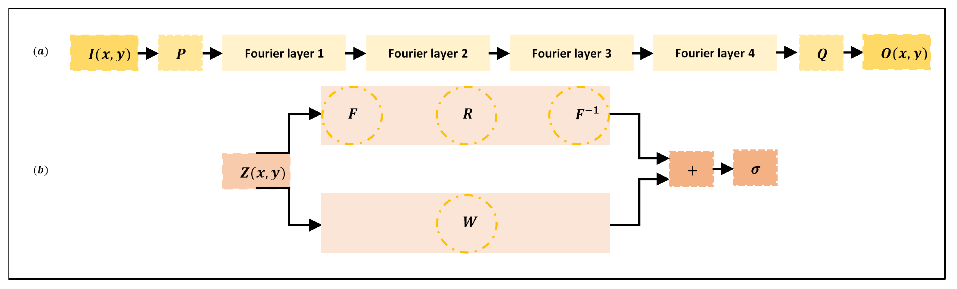
At any location within a mesh, the FNO algorithm first raises the input to a higher-dimension channel space , where (Figure 1). It does this by locally applying the transform , with a parametric procedure using either a Fully Connected (FC) neural network or a simple linear layer. is defined on the similar mesh to I and the values of can be displaced as an image with channels. Then, four successive Fourier layers are applied to . Subsequently, another transform is applied locally . This final transform projects to the output by ). Meantime, is the output of the fourth (final) Fourier layer and Q is parameterized by a fully connected neural network.
passes through two routes in the Fourier layers. In the top path, a Fourier transform F, a linear transform R on the lower Fourier modes, and an inverse Fourier transform are applied. undergoes only a local linear transform W in the bottom path. Outputs of each path are added together and then subjected to an activation function (here ReLu).
To establish an optimum FNO architecture, PyTorch [28] was employed with Python version 3.9.12. The models developed for the dataset applied batch size = 5, epochs = 500, step size = 100, gamma = 0.9, and downsampling rate = 1 in this research. Additionally, ‘Adam’ [29] was used as the optimizer with a learning rate of 0.001 and a weight decay of 0.0001. Adam uses a distinct learning rate for each scalar parameter and adapts these rates during the whole training process considering the historical values of the partial derivatives of each parameter. This gradient-based algorithm combines the ability of (i) AdaGrad to handle sparse gradients and (ii) RMSProp to function in online and non-stationary settings. The input and output shapes defined were 30 × 30 × 1 and 30 × 30, respectively. Moreover, fast Fourier transform [30] was used as a fast algorithm to compute discrete Fourier transforms and their inverses.
3.2. CNN Architecture
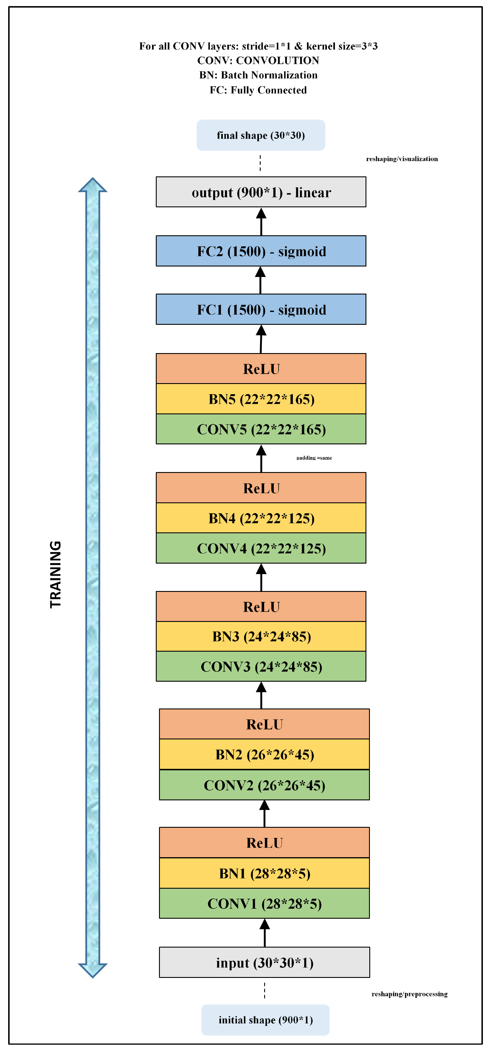
In preparing a CNN simulation involving a unit square, a 30 × 30 uniform mesh was selected. On the other hand, the input/output values were defined as a 900 × 1 1D tensor (vector). The input shape was then changed to 30 × 30 × 1 for processing through 2D convolutional filters. Regarding to the output in CNN, there were two options: keeping the initial shape or reshaping to a 2D tensor. While reshaping to 30 × 30, the accuracy achieved by the CNN model became substantially impaired. On the other hand, many fewer errors were generated by CNN models that retained the initial 900 × 1 shape. Therefore, the CNN model was developed and its computational layers processed with the 900 × 1 shape and only reshaped to the 30 × 30 output size for final visualization purposes (Figure 2).
An optimum CNN architecture was developed with five convolutional layers and two FC layers (Figure 2). The kernel numbers in the convolutional layers (referred to as CONV1 to CONV5) were 5, 45, 85, 125, and 165, respectively. Padding was set to ‘same’ only in CONV5 to prevent the size from changing. A 3 × 3 kernel size and 1 × 1 stride were applied to all convolutional layers, providing those layers with sizes 28 × 28, 26 × 26, 24 × 24, 22 × 22, and 22 × 22, respectively. A batch normalization layer (referred to as BN1 to BN5) followed CONV1 to CONV5, without changing size. Normalization of the input layer makes the CNN converge more quickly to outputs that collectively average nearly zero with a standard deviation of nearly one. The layers FC1 and FC2 contain 1500 neurons. The ReLu activation function was applied to CONV1 to CONV5, whereas the sigmoid activation function was applied to FC1 and FC2, with a linear transformation applied to generate the output layer.
The CNN model was coded using the Keras/TensorFlow packages [31] executed in virtual environments in Python version 3.9.12. It was specifically configured with the Mean Squared Error (MSE) as the loss (objective) function and ‘Adam’ [29] with the default values as the optimizer. The CNN was trained to apply a batch size of 16 samples and run with 500 epochs.
4. Results
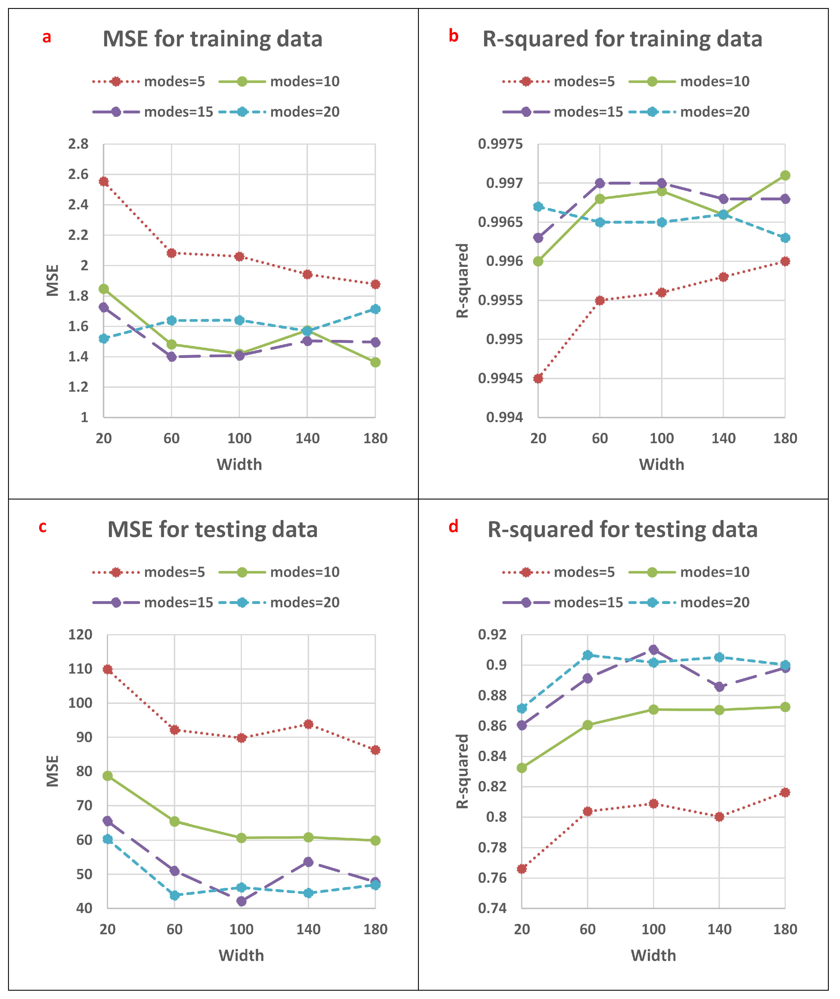
There are two main hyperparameters in FNO: the number of channels and modes. The former defines the width of the FNO network, referring to the number of features learned in each layer. The latter defines the number of lower Fourier modes retained when truncating the Fourier series. The size of the grid space controls the maximum allowable number of modes. In this research, five values were evaluated for the width: 20, 60, 100, 140, and 180, and four cases were evaluated for the mode: 5, 10, 15, and 20.
Figure 3a reveals that the FNO models generated very similar errors, based on MSE, when calculated based on initial pressure values (actual non-normalized values) for the training data when the number of modes is 10, 15, or 20. However, the errors increased slightly for models configured with . The coefficient of determination (R) values for the training data varied from 0.9945 to 0.9971, according to Figure 3b. As a general result, all models were able to predict pressure with acceptable error levels for the training subset.
Figure 3c,d display the FNO results for the testing subset. The model with modes of 5 generated the poorest prediction performance, i.e., highest MSE and lowest R. As width increased (with modes held at 5), MSE decreased from 109.9231 to 86.3347 and R increased from 0.7661 to 0.8163. When the number of modes was increased to 10, the FNO performance improved. Additionally, an increase in width had a positive effect on accuracy when modes were held at 10. The model with performed better than models with modes of 5 or 10, as it generated MSE and R displaying ranges of 42.1611–65.5664 and 0.8605–0.9103, respectively. In general, the prediction performance of the FNO model with modes of 20 overlapped with that of modes of 15. Considering all twenty cases, the model with and generated the best performance with an MSE of 1.4087 and R of 0.997 for the training subset, and an MSE of 42.1611 and R of 0.9103 for the testing subset. In addition to the graphical comparisons (Figure 3), the MSE and R values achieved by all FNO cases evaluated are listed in Table 1.
To assess whether downsampling has a positive or negative impact on the FNO model performance with respect to small-shape data (in the dataset modeled: 30 × 30), a downsampling rate was set to 2. By applying that rate, the data shape was reduced to 15 × 15, which led to poor prediction results. For example, with and , the FNO model achieved pressure predictions with MSE of 27.3128 and R of 0.9411 for the training subset, and with MSE of 410.7709 and R of 0.1259 for the testing subset. As to be expected, further downsampling of the initial case caused prediction accuracy to deteriorate further. A likely explanation for this outcome is that the size of the grid space controls the maximum allowable number of modes. This means that by downsampling, the allowable number of FNO modes also decreases. Meantime, because CNN acts on discretized vectors, downsampling with CNN is not reasonable.
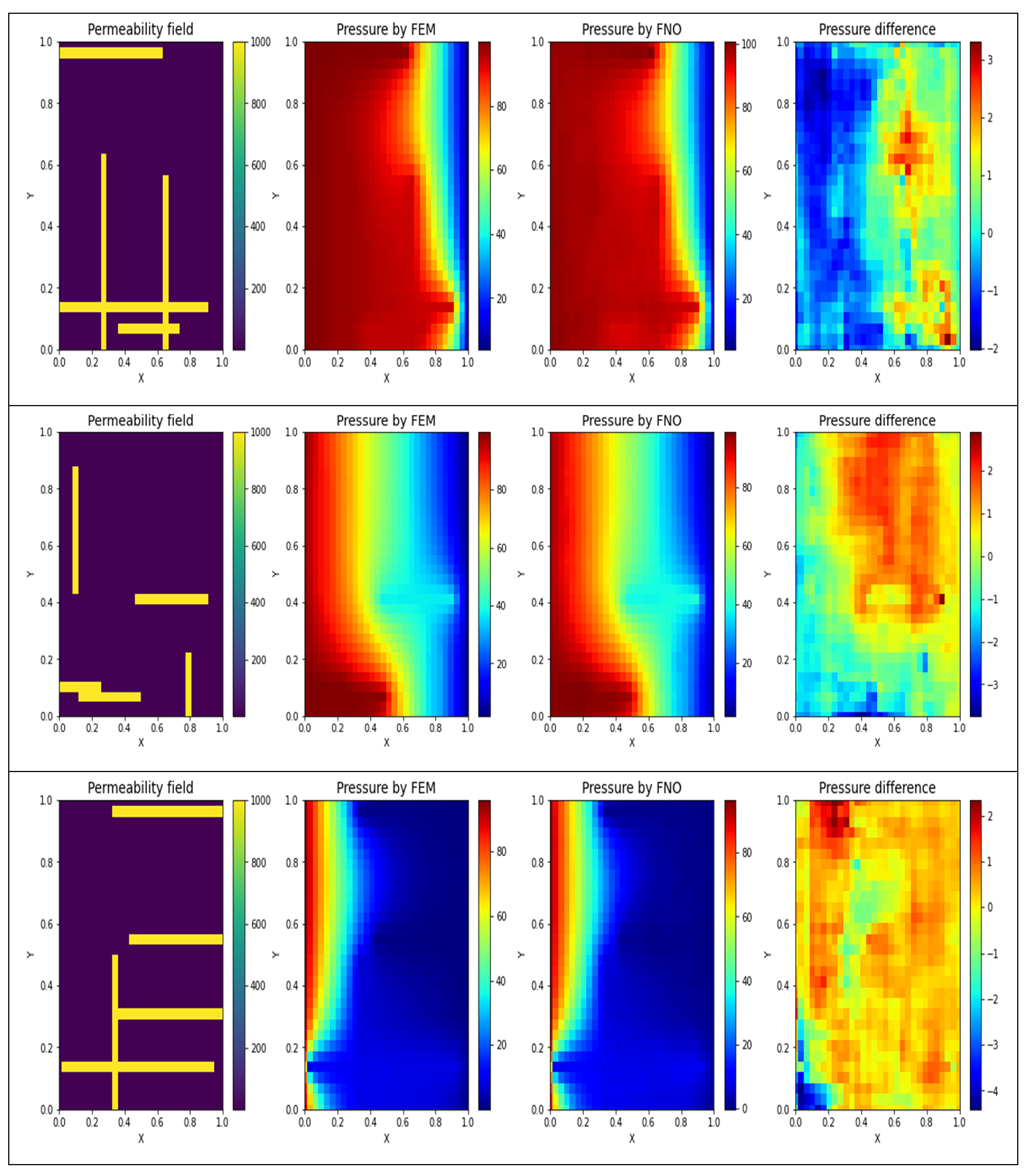
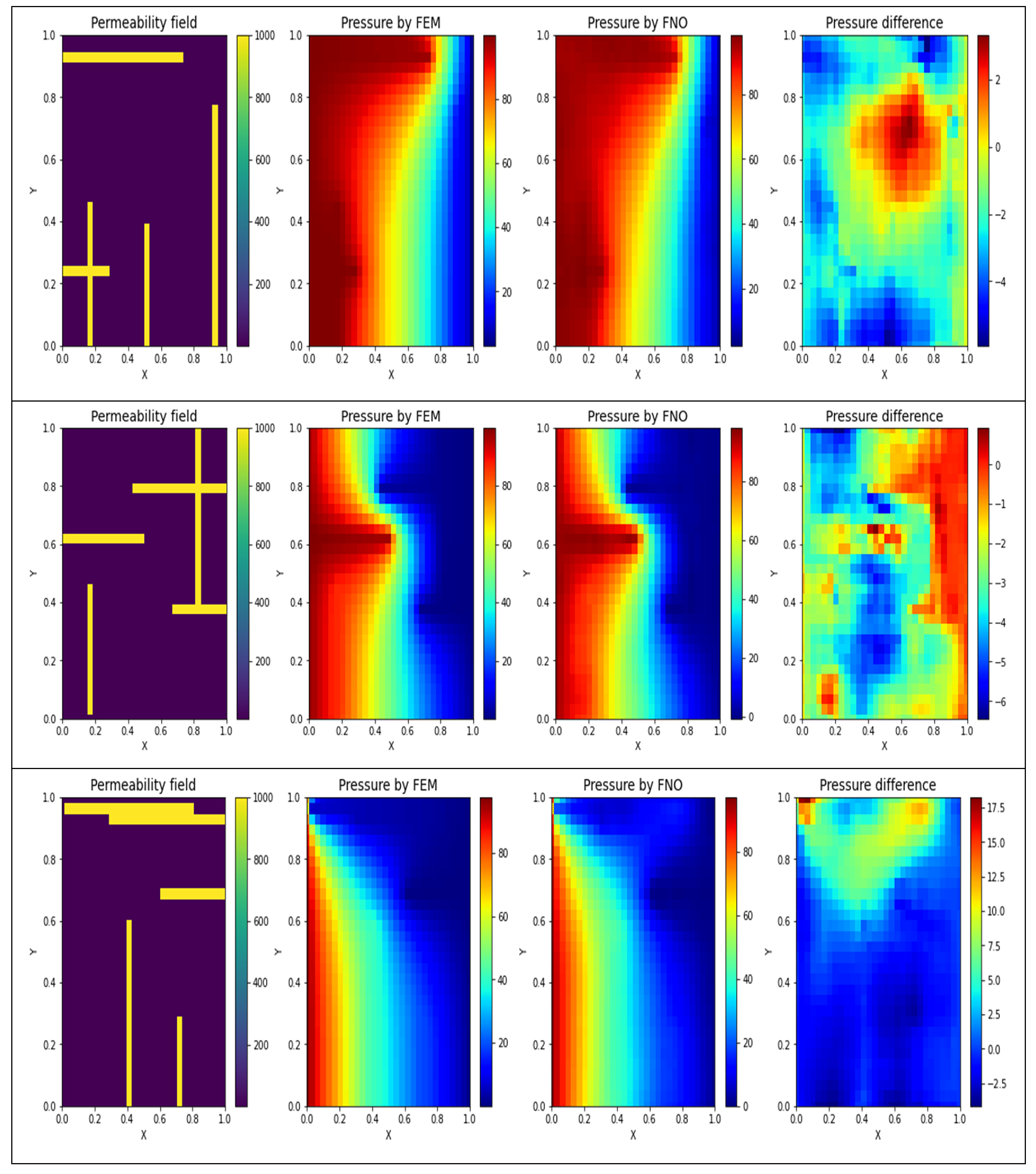
In order to improve visualization of the pressure changes occurring over the defined shapes, three examples are illustrated for selected training (Figure 4) and testing (Figure 5) subsets. The plots in the left-side columns display the permeability fields, for representative sample grids. The plots in the left-central columns display the pressure distribution derived by FEM (considered to be true distribution). The plots in the right-central columns display the predicted pressure distributions of the best-performing FNO model developed. The plots in the right-side columns display the pressure difference between the FEM and FNO outputs []. Generally, there was a very close match between the true pressure distributions and those predicted by the FNO model, especially for the training dataset.
The prediction performance of the CNN model is similar to that of the FNO model in terms of R with regard to the training subset (Table 2). Indeed, the MSE generated by the CNN model (0.3074) is slightly less than that generated by the FNO model (1.4087). Nonetheless, the FNO model clearly provided superior results in terms of R and MSE when the trained models were applied to the testing data subset. The results (Table 2) suggest that whereas the trained FNO model is well-fitted to the dataset, the trained CNN model is somewhat over-fitted to the same dataset.
5. Discussion
The FNO model is underpinned by a rigorous mathematical methodology, as described. Furthermore, the statistical/graphical pressure prediction results associated with the small-size grids simplistically simulating fluid flow in a subsurface reservoir indicate promising prediction accuracy, which outperforms that of a CNN model. However, there is a drawback associated with the FNO model applied to these small-size grids. As with other data-driven ML/DL methods, FNO relies on the number of data samples it is provided with, and it may require a large number of small-size grids to adequately train it to fully learn the full range of possible variations in complex subsurface systems. For this reason, FNO was applied to a relatively simple example dataset, i.e., based on relatively limited assumptions of md, md, and . As opposed to data-driven neural networks such as FNO, which rely exclusively on the provided data points, Physics-Informed Neural Networks (PINNs) use the PDE itself as a data source. In PINNs, the PDEs are explicitly encoded into the NN via automatic differentiation algorithms. The weighted summation of the MSE of the PDE residuals, BCs, ICs, and possibly known solution points could then be minimized as a loss function based on the NN parameters. Therefore, it could be beneficial to combine PINN and FNO to find out how the performance changes compared to a stand-alone FNO. In this sense, the model uses available data and/or physics constraints to learn the solution operator, conquering the limitations of purely data-driven and physics-based techniques.
6. Conclusions
Classical NNs attempt to learn mappings between finite-dimensional Euclidean spaces, making them confined to a particular discretization. On the other hand, the FNO, as a mesh-independent algorithm, tries to learn function-to-function mappings. This makes it possible for FNO to be trained on one mesh and subsequently assessed on another. This study further extended the capabilities of FNO by applying it to a new simulated dataset made up of small-shape samples. The generated dataset simulates single-phase fluid flow in a porous reservoir assessed by 1700 2D grid samples, each constructed as a unit square with a 30 × 30 uniform mesh. The models of FNO and CNN are trained to predict the pressure distribution of each grid sample based on its permeability field. The statistical-graphical results confirm the good ability of the FNO to predict the pressure distribution based on the permeability field. The FNO model provided better prediction performance than the CNN model when applied to the testing dataset. Analysis of the results leads to three recommendations for future research. These are: (i) training the FNO models for fluid flow in porous media with more data covering a wider range of matrix and fracture permeabilities and a variable number of fractures in each small-shape grid sample, (ii) applying FNO to solve other types of small-shape data problems, and (iii) designing and testing novel more complex FNO architectures.
Author Contributions
Conceptualization, A.C. and J.C.; methodology, A.C.; formal analysis, A.C., J.C. and D.A.W.; data curation, A.C. and J.C.; writing original draft, A.C.; writing—review and editing by A.C., D.A.W. and F.C.; visualization, A.C.; supervision, J.C., F.C. and F.M. All authors have read and agreed to the published version of the manuscript.
Funding
This work is partially supported by the Key Program Special Fund in XJTLU (KSF-E-50), XJTLU Postgraduate Research Scholarship (PGRS1912009), and XJTLU Research Development Funding (RDF-19-01-15).
Institutional Review Board Statement
Not applicable.
Informed Consent Statement
Not applicable.
Data Availability Statement
The datasets generated and supporting the findings of this article are obtainable from the corresponding author(s) upon reasonable request.
Acknowledgments
We would like to thank Zongyi Li for clarifying some points related to FNO.
Conflicts of Interest
The authors declare no conflict of interest.
Abbreviations
The following abbreviations are used in this manuscript:
| first term of | |
| Fourier series coefficient | |
| BC | Boundary Condition |
| BN | Batch Normalization |
| Fourier series coefficient | |
| CNN | Convolutional Neural Network |
| CONV | convolutional layers |
| DL | Deep Learning |
| Laplace pressure | |
| f | source term |
| F | Fourier transform |
| inverse Fourier transform | |
| FC | Fully Connected |
| FEM | Finite Element Method |
| FNO | Fourier Neural Operator |
| i | imaginary number () |
| IC | Initial Condition |
| input layer | |
| permeability of the fracture | |
| permeability of the matrix | |
| LES | Large Eddy Simulation |
| ML | Machine Learning |
| number of fractures | |
| MSE | Mean Squared Error |
| fluid viscosity | |
| NN | Neural Network |
| gradient pressure | |
| divergence velocity | |
| ODE | Ordinary Differential Equation |
| output layer | |
| PDE | Partial Differential Equation |
| PINN | Physics-Informed Neural Network |
| R | linear transform |
| R | coefficient of determination |
| s | angular frequency |
| k | permeability |
| u | Darcy velocity |
| W | local linear transform |
| higher-dimension channel space | |
| output of the fourth (final) Fourier layer |
References
- Golub, G.H.; Ortega, J.M. Scientific Computing and Differential Equations: An Introduction to Numerical Methods; Academic Press: Cambridge, MA, USA, 1992. [Google Scholar]
- Tao, Z.; Cui, Z.; Yu, J.; Khayatnezhad, M. Finite difference modelings of groundwater flow for constructing artificial recharge structures. Iran. J. Sci. Technol. Trans. Civ. Eng. 2022, 46, 1503–1514. [Google Scholar] [CrossRef]
- Fathollahi, R.; Hesaraki, S.; Bostani, A.; Shahriyari, E.; Shafiee, H.; Pasha, P.; Chari, F.N.; Ganji, D.D. Applying numerical and computational methods to investigate the changes in the fluid parameters of the fluid passing over fins of different shapes with the finite element method. Int. J. Thermofluids 2022, 15, 100187. [Google Scholar] [CrossRef]
- Afzal, A.; Saleel, C.A.; Prashantha, K.; Bhattacharyya, S.; Sadhikh, M. Parallel finite volume method-based fluid flow computations using OpenMP and CUDA applying different schemes. J. Therm. Anal. Calorim. 2021, 145, 1891–1909. [Google Scholar] [CrossRef]
- Han, C.; Wang, Y.L.; Li, Z.Y. Numerical Solutions of Space Fractional Variable-Coefficient Kdv–Modified Kdv Equation by Fourier Spectral Method. Fractals 2021, 29, 2150246. [Google Scholar] [CrossRef]
- Bhardwaj, A.; Kumar, A. A meshless method for time fractional nonlinear mixed diffusion and diffusion-wave equation. Appl. Numer. Math. 2021, 160, 146–165. [Google Scholar] [CrossRef]
- Keybondorian, E.; Soltani Soulgani, B.; Bemani, A. Application of ANFIS-GA algorithm for forecasting oil flocculated asphaltene weight percentage in different operation conditions. Pet. Sci. Technol. 2018, 36, 862–868. [Google Scholar] [CrossRef]
- Mohammadi, M.; Safari, M.; Ghasemi, M.; Daryasafar, A.; Sedighi, M. Asphaltene adsorption using green nanocomposites: Experimental study and adaptive neuro-fuzzy interference system modeling. J. Pet. Sci. Eng. 2019, 177, 1103–1113. [Google Scholar] [CrossRef]
- Mai, H.; Le, T.C.; Chen, D.; Winkler, D.A.; Caruso, R.A. Machine learning for electrocatalyst and photocatalyst design and discovery. Chem. Rev. 2022, 122, 13478–13515. [Google Scholar] [CrossRef] [PubMed]
- Kazemi, P.; Ghisi, A.; Mariani, S. Classification of the Structural Behavior of Tall Buildings with a Diagrid Structure: A Machine Learning-Based Approach. Algorithms 2022, 15, 349. [Google Scholar] [CrossRef]
- Chen, W.; Wang, S.; Zhang, X.; Yao, L.; Yue, L.; Qian, B.; Li, X. EEG-based motion intention recognition via multi-task RNNs. In Proceedings of the 2018 SIAM International Conference on Data Mining, SIAM, San Diego, CA, USA, 3–5 May 2018; pp. 279–287. [Google Scholar]
- Choubineh, A.; Chen, J.; Coenen, F.; Ma, F. An innovative application of deep learning in multiscale modeling of subsurface fluid flow: Reconstructing the basis functions of the mixed GMsFEM. J. Pet. Sci. Eng. 2022, 216, 110751. [Google Scholar] [CrossRef]
- Choubineh, A.; Chen, J.; Coenen, F.; Ma, F. A quantitative insight into the role of skip connections in deep neural networks of low complexity: A case study directed at fluid flow modeling. J. Comput. Inf. Sci. Eng. 2022, 23, 014502. [Google Scholar] [CrossRef]
- Pawar, P.; Ainapure, B.; Rashid, M.; Ahmad, N.; Alotaibi, A.; Alshamrani, S.S. Deep Learning Approach for the Detection of Noise Type in Ancient Images. Sustainability 2022, 14, 11786. [Google Scholar] [CrossRef]
- Mijalkovic, J.; Spognardi, A. Reducing the False Negative Rate in Deep Learning Based Network Intrusion Detection Systems. Algorithms 2022, 15, 258. [Google Scholar] [CrossRef]
- Li, Z.; Kovachki, N.; Azizzadenesheli, K.; Liu, B.; Bhattacharya, K.; Stuart, A.; Anandkumar, A. Fourier neural operator for parametric partial differential equations. arXiv 2020, arXiv:2010.08895. [Google Scholar]
- Gallant, A.R.; White, H. There exists a neural network that does not make avoidable mistakes. In Proceedings of the ICNN, San Diego, CA, USA, 24–27 July 1988; pp. 657–664. [Google Scholar]
- Silvescu, A. Fourier neural networks. In Proceedings of the IJCNN’99, International Joint Conference on Neural Networks, Proceedings (Cat. No. 99CH36339), Washington, DC, USA, 10–16 July 1999; Volume 1, pp. 488–491. [Google Scholar]
- Liu, S. Fourier neural network for machine learning. In Proceedings of the 2013 International Conference on Machine Learning and Cybernetics, Tianjin, China, 14–17 July 2013; Volume 1, pp. 285–290. [Google Scholar]
- Wen, G.; Li, Z.; Azizzadenesheli, K.; Anandkumar, A.; Benson, S.M. U-FNO—An enhanced Fourier neural operator-based deep-learning model for multiphase flow. Adv. Water Resour. 2022, 163, 104180. [Google Scholar] [CrossRef]
- Rashid, M.M.; Pittie, T.; Chakraborty, S.; Krishnan, N.A. Learning the stress-strain fields in digital composites using fourier neural operator. iScience 2022, 105452. [Google Scholar] [CrossRef] [PubMed]
- Li, Z.; Peng, W.; Yuan, Z.; Wang, J. Fourier neural operator approach to large eddy simulation of three-dimensional turbulence. Theor. Appl. Mech. Lett. 2022, 100389. [Google Scholar] [CrossRef]
- Johnny, W.; Brigido, H.; Ladeira, M.; Souza, J.C.F. Fourier Neural Operator for Image Classification. In Proceedings of the 2022 17th Iberian Conference on Information Systems and Technologies (CISTI), Madrid, Spain, 22–25 June 2022; pp. 1–6. [Google Scholar]
- Chen, Z. Reservoir Simulation: Mathematical Techniques in Oil Recovery; SIAM: Philadelphia, PA, USA, 2007. [Google Scholar]
- Fukunaga, K.; Koontz, W.L. Application of the Karhunen-Loeve expansion to feature selection and ordering. IEEE Trans. Comput. 1970, 100, 311–318. [Google Scholar] [CrossRef] [Green Version]
- Lasser, R. Introduction to Fourier Series; CRC Press: Boca Raton, FL, USA, 1996; Volume 199. [Google Scholar]
- Strichartz, R.S. A Guide to Distribution Theory and Fourier Transforms; World Scientific Publishing Company: Hackensack, NJ, USA, 2003. [Google Scholar]
- Subramanian, V. Deep Learning with PyTorch: A Practical Approach to Building Neural Network Models Using PyTorch; Packt Publishing Ltd.: Birmingham, UK, 2018. [Google Scholar]
- Reddi, S.J.; Kale, S.; Kumar, S. On the convergence of adam and beyond. arXiv 2019, arXiv:1904.09237. [Google Scholar]
- Nussbaumer, H.J. The fast Fourier transform. In Fast Fourier Transform and Convolution Algorithms; Springer: Berlin/Heidelberg, Germany, 1981; pp. 80–111. [Google Scholar]
- Joseph, F.J.J.; Nonsiri, S.; Monsakul, A. Keras and TensorFlow: A hands-on experience. In Advanced Deep Learning for Engineers and Scientists; Springer: Cham, Switzerland, 2021; pp. 85–111. [Google Scholar]
Figure 1.
(a) Architecture of the neural operator and (b) Architecture of a Fourier layer.

Figure 2.
The structure of the CNN model used in this study.

Figure 3.
Prediction error graphical analysis of the developed FNO models: (a) MSE for training data, (b) R for training data, (c) MSE for testing data, and (d) R for testing data.
Figure 3.
Prediction error graphical analysis of the developed FNO models: (a) MSE for training data, (b) R for training data, (c) MSE for testing data, and (d) R for testing data.

Figure 4.
A comparison between the actual pressure distributions and those obtained by FNO for three representative training subset samples. The pressure difference is based on a point-by-point absolute error. Outputs are displayed as rectangles rather than squares due to a scaling issue.
Figure 4.
A comparison between the actual pressure distributions and those obtained by FNO for three representative training subset samples. The pressure difference is based on a point-by-point absolute error. Outputs are displayed as rectangles rather than squares due to a scaling issue.

Figure 5.
A comparison between the actual pressure distributions and those obtained by FNO for three representative testing subset samples. The pressure difference is based on a point-by-point absolute error. Outputs are displayed as rectangles rather than squares due to a scaling issue.
Figure 5.
A comparison between the actual pressure distributions and those obtained by FNO for three representative testing subset samples. The pressure difference is based on a point-by-point absolute error. Outputs are displayed as rectangles rather than squares due to a scaling issue.


Table 1.
Performance of the developed FNO models with different modes and widths based on MSE and R.
Table 1.
Performance of the developed FNO models with different modes and widths based on MSE and R.
| Mode | Width | MSE (Training) | R (Training) | MSE (Testing) | R (Testing) |
|---|---|---|---|---|---|
| 5 | 20 | 2.5543 | 0.9945 | 109.9231 | 0.7661 |
| 5 | 60 | 2.0832 | 0.9955 | 92.2014 | 0.8038 |
| 5 | 100 | 2.0605 | 0.9956 | 89.8219 | 0.8089 |
| 5 | 140 | 1.943 | 0.9958 | 93.8539 | 0.8003 |
| 5 | 180 | 1.878 | 0.996 | 86.3347 | 0.8163 |
| 10 | 20 | 1.8483 | 0.996 | 78.7648 | 0.8324 |
| 10 | 60 | 1.4814 | 0.9968 | 65.4587 | 0.8607 |
| 10 | 100 | 1.4196 | 0.9969 | 60.6803 | 0.8709 |
| 10 | 140 | 1.5745 | 0.9966 | 60.8775 | 0.8705 |
| 10 | 180 | 1.3643 | 0.9971 | 59.8904 | 0.8726 |
| 15 | 20 | 1.7253 | 0.9963 | 65.5664 | 0.8605 |
| 15 | 60 | 1.4007 | 0.997 | 51.0625 | 0.8914 |
| 15 | 100 | 1.4087 | 0.997 | 42.1611 | 0.9103 |
| 15 | 140 | 1.505 | 0.9968 | 53.6779 | 0.8858 |
| 15 | 180 | 1.4966 | 0.9968 | 47.783 | 0.8983 |
| 20 | 20 | 1.5206 | 0.9967 | 60.3367 | 0.8716 |
| 20 | 60 | 1.6387 | 0.9965 | 43.8621 | 0.9067 |
| 20 | 100 | 1.6409 | 0.9965 | 46.167 | 0.9018 |
| 20 | 140 | 1.5687 | 0.9966 | 44.5223 | 0.9053 |
| 20 | 180 | 1.7145 | 0.9963 | 46.8985 | 0.9002 |
Table 2.
A comparison between the performance of the best-performing FNO model and the CNN model in terms of MSE and R.
Table 2.
A comparison between the performance of the best-performing FNO model and the CNN model in terms of MSE and R.
| Model | MSE (Training) | R (Training) | MSE (Testing) | R (Testing) |
|---|---|---|---|---|
| FNO ( and ) | 1.4087 | 0.997 | 42.1611 | 0.9103 |
| CNN | 0.3074 | 0.9993 | 86.1818 | 0.8166 |
Disclaimer/Publisher’s Note: The statements, opinions and data contained in all publications are solely those of the individual author(s) and contributor(s) and not of MDPI and/or the editor(s). MDPI and/or the editor(s) disclaim responsibility for any injury to people or property resulting from any ideas, methods, instructions or products referred to in the content. |
© 2023 by the authors. Licensee MDPI, Basel, Switzerland. This article is an open access article distributed under the terms and conditions of the Creative Commons Attribution (CC BY) license (https://creativecommons.org/licenses/by/4.0/).
Share and Cite
MDPI and ACS Style
Choubineh, A.; Chen, J.; Wood, D.A.; Coenen, F.; Ma, F. Fourier Neural Operator for Fluid Flow in Small-Shape 2D Simulated Porous Media Dataset. Algorithms 2023, 16, 24. https://doi.org/10.3390/a16010024
AMA Style
Choubineh A, Chen J, Wood DA, Coenen F, Ma F. Fourier Neural Operator for Fluid Flow in Small-Shape 2D Simulated Porous Media Dataset. Algorithms. 2023; 16(1):24. https://doi.org/10.3390/a16010024
Chicago/Turabian StyleChoubineh, Abouzar, Jie Chen, David A. Wood, Frans Coenen, and Fei Ma. 2023. "Fourier Neural Operator for Fluid Flow in Small-Shape 2D Simulated Porous Media Dataset" Algorithms 16, no. 1: 24. https://doi.org/10.3390/a16010024
Note that from the first issue of 2016, this journal uses article numbers instead of page numbers. See further details here.