
Improvement of Ant Colony Algorithm Performance for the Job-Shop Scheduling Problem Using Evolutionary Adaptation and Software Realization Heuristics


Ural Power Engineering Institute, Ural Federal University named after the first President of Russia B.N. Yeltsin, 620002 Ekaterinburg, Russia
Algorithms 2023, 16(1), 15; https://doi.org/10.3390/a16010015
Submission received: 25 November 2022
/
Revised: 20 December 2022
/
Accepted: 22 December 2022
/
Published: 26 December 2022
(This article belongs to the Special Issue Bio-Inspired Algorithms)
Abstract
:Planning tasks are important in construction, manufacturing, logistics, and education. At the same time, scheduling problems belong to the class of NP-hard optimization problems. Ant colony algorithm optimization is one of the most common swarm intelligence algorithms and is a leader in solving complex optimization problems in graphs. This paper discusses the solution to the job-shop scheduling problem using the ant colony optimization algorithm. An original way of representing the scheduling problem in the form of a graph, which increases the flexibility of the approach and allows for taking into account additional restrictions in the scheduling problems, is proposed. A dynamic evolutionary adaptation of the algorithm to the conditions of the problem is proposed based on the genetic algorithm. In addition, some heuristic techniques that make it possible to increase the performance of the software implementation of this evolutionary ant colony algorithm are presented. One of these techniques is parallelization; therefore, a study of the algorithm’s parallelization effectiveness was made. The obtained results are compared with the results of other authors on test problems of scheduling. It is shown that the best heuristics coefficients of the ant colony optimization algorithm differ even for similar job-shop scheduling problems.
1. Introduction
1.1. Job-Shop Scheduling Problem
In all cases of human activity to achieve the desired result, as a rule, plans and schedules are drafted. The complexity of task scheduling along with the continuous improvement of automation tools for such activities has led to increased interest in scheduling synthesis theory and calendar planning. The tasks of calendar planning reflect the process of the distribution over time of a limited number of resources assigned to the project, which includes a list of related works.
Problems of scheduling theory belong to the class of problems of combinatorial optimization or ordering. The active research and development of scheduling theory began in the 1950s. One of the main issues of scheduling theory was the classification of tasks and the establishment of their complexity. Reviews of problems in scheduling theory are presented in the works of Gary and Johnson, Lower, Brucker, Xie, Leusin, and Xiong, et al. [1,2,3,4,5,6].
The scheduling problem of the “job-shop” class is NP-hard if there are more than two devices [5,7]. The survey [6] shows that the job-shop scheduling (JSS) problem is one of the most difficult among all NP-class problems even from the point of view of task formulation. As shown in [8], the number of combinations for a job-shop task with n jobs and m devices (each job contains m stages) is proportional to the value (n!)m. At the same time, JSS problems are important for many fields: manufacturing, semiconductors, pharmaceuticals, supply chains, rail-bound transportation, mining, healthcare, etc. [6].
Since planning tasks are very important in practice and have high complexity and variety, a wide variety of methods are used to solve them, including artificial intelligence methods [5,9,10]. Although classical optimization methods are also used, such as the branch and bound method [11,12], dynamic programming [7], and methods based on heuristics and rules [13,14,15,16].
Among the methods of artificial intelligence, the most commonly used is the genetic algorithm (GA) [5,17,18,19] and other population-based algorithms such as the Particle Swarm Optimization [20,21] and ant colony optimization (ACO) algorithms [22]. All these stochastic population optimization algorithms (evolutionary or swarm) provide high flexibility and solve scheduling problems not with 100% accuracy but with sufficient accuracy in a reasonable time. In addition, population algorithms can be used to create hybrids with other, deterministic approaches [7,17,18,19,23]. Additionally worthy of note is the use of stochastic algorithms that are faster than population algorithms and based on Simulated Annealing [10,24].
Despite a large number of solution methods, none of them can be called dominant. Besides the usual reasons typical for NP-hard problems [25], the variability of planning problems even within the same class should also be noted.
Most scheduling tasks are associated with the concept of multi-stage service systems. These include systems in which servicing requirements consist of several stages. Despite the diversity of production systems, the formalized description of the JSS problem can be considered basic for a large class of multi-stage systems. The job-shop problem can be formulated as follows.
1. There is a finite set N = {1, 2, …, n} of requirements (works, jobs, orders) and a finite set M = {1, 2, …, m} of devices (machines, executors, workstations, etc.).
The service process for requirement i includes ri stages. At the same time, each requirement i and each stage q (1 ≤ q ≤ ri) of its service is associated with some subset of machines Miq from the set M. It is assumed that each machine can simultaneously serve no more than one requirement. In such systems with successive servers, each job i is assigned its own, characterizing for this job the sequence Li of its servicing by machines: Li = (L1i, L2i, …, Lrii).
The requirement i is served first by the machine L1i, then by L2i, and so on. Service sequences may be different for different requirements and may contain instrument repetitions. If the requirement i at stage q must be serviced by machine l, then the duration tliq of its servicing by this machine is assumed to be given. The system operation process can be described by setting a schedule (calendar plan), i.e., some set of indications as to whether particular requirements are served at each moment of time.
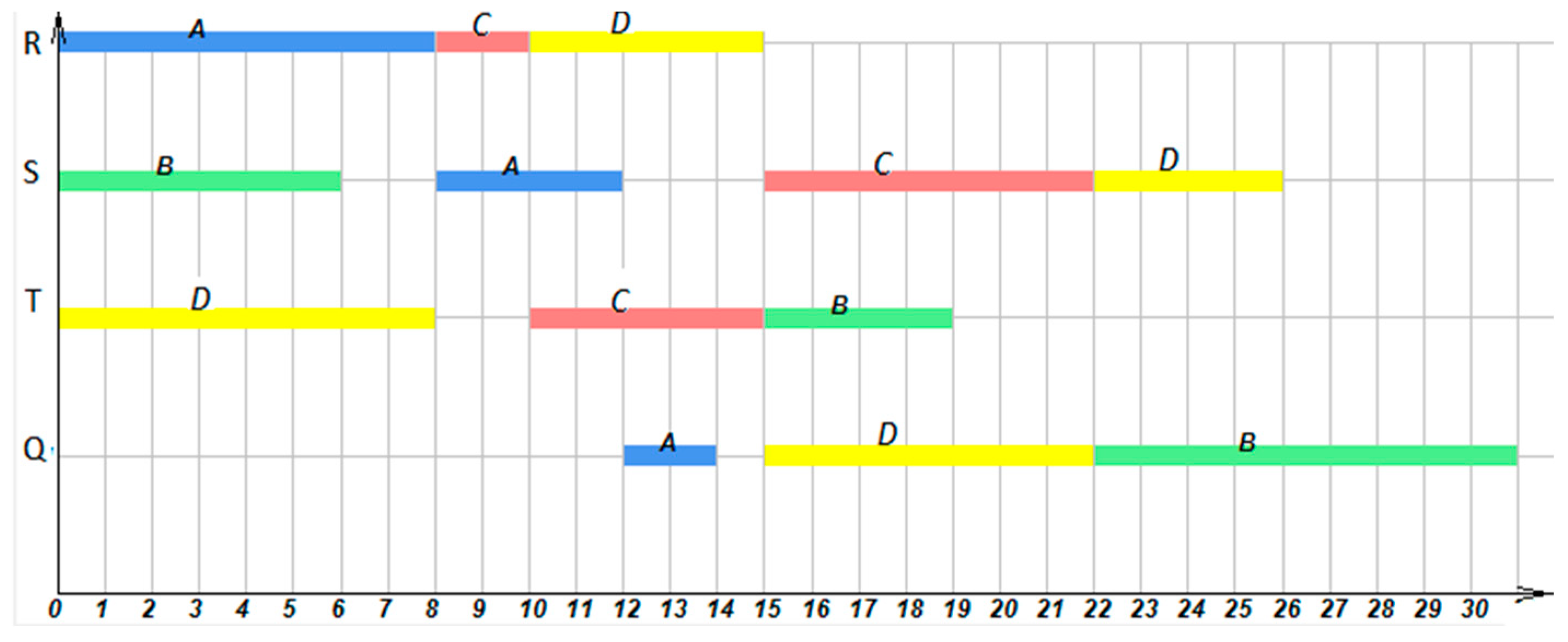
Figure 1 shows a Gantt chart of an example of a JSS problem with jobs A (blue), B (green), C (red), and D (yellow) and machines R, S, T, and Q. For example, job A has three stages that require the consistent use of machines R (8 h), S (5 h), and Q (2 h).
Under the assumptions made above, the schedule can be considered a vector {s1(t), s1(t), …, sm(t)}, whose components are piecewise constant left continuous functions. Each of them is given on the interval 0 ≤ t < ∞ and takes a value of 0, 1, …, n.
s = {s1(t), s2(t), …, sm(t)}.
If (t′) = i, l ∈ M, i ∈ N, then at the time t′, the device l serves the requirement i. When setting the schedule, all conditions and restrictions arising from the formulation of the problem under consideration must be observed, which means the schedule must be permissible.
If there are several permissible schedules, it is necessary to choose the best of them, which means setting some selection criterion (quality criterion). In the classical scheduling theory, such a criterion is the completion time of all requirements (makespan); that is, the completion time of the last requirement. Each admissible schedule s uniquely determines the vector of time points for completing the service of all jobs:
T(s) = (T1(s), T2(s), …, Tn(s)).
If some valid, non-decreasing in each of the variables function F(x) is given,
then the quality of the schedule s is estimated by the value of this function at x = T(s):
F(x) = F(x1, x2, …, xn),
F(x) = max{xi}, i = 1,2, …, n.
In this case,
F(T(s)) = Tmax(s), where Tmax(s) = max{Ti(s)}, i = 1, 2, …, n,
From this statement of the problem, the main difficulties are noticeable:
- Discreteness;
- Multivariance;
- Multifactorialism;
- The inability to construct an objective function in the form of an algebraic expression, since the objective function is calculated only algorithmically.
Mathematically, the JSS problem can be divided into several subtypes according to their constrictions, criteria, and other features. The review [6] identifies 37 subtypes of the JSS problem. It also provides mathematical formulations for various subtypes and a review of solution methods. A variety of tasks and methods and the fact that research on this issue does not stop indicate both the relevance and high complexity of the JSS problem.
1.2. Ant Colony Optimization Algorithm
Ants solve pathfinding problems using chemical regulation [26]. Each ant leaves a trail of special substances on the ground (named pheromones). Another ant, sensing a footprint on the ground, rushes along it. The more ants have passed along one path, the more noticeable the trace for them, and the more noticeable the trace, the greater the desire to go in the same direction arises in ants. Since the ants that find the shortest path to the “feeder” spend less time traveling back and forth, their trail quickly becomes the most visible. It attracts more ants, so the process of finding a shorter path is completed quickly. Other, less-used paths gradually disappear. It is possible to formulate the basic principles of interaction between ants: stochastic; multiplicity; positive feedback.
Since each ant performs primitive actions, the algorithm turns out to be very simple and boils down to multiple traversals of some graph, the edges of which have not only weight but also an additional, dynamically changing quantitative characteristic, called the amount of pheromone or simply pheromone.
The ACO algorithm is inherently the most suitable for solving optimization problems related to graphs and routes [26,27,28,29]. Currently, research related to the ACO algorithm is aimed at solving problems such as finding an efficient starting point [28,29], hybridization with other methods that solve subproblems (local search [30,31], exact large neighborhood search [32], etc.), the usage of adaptation methods, and the meta-optimization of the algorithm [33,34]. The application of the local search and neighborhood search [30,31,32] is difficult for JSS problems because of their non-trivial formulation [6].
Research in which the ACO algorithm would be applied to scheduling problems began as soon as ACO algorithms became known; for example, the application of ACO to single-machine scheduling problems [35,36] or JSS problems in general [37]. In particular, authors use techniques for combining the ACO algorithm and specialized methods for solving JSS problems; for example, to perform local searches [38,39]. The JSS problem differs significantly from route search problems and other problems on graphs. In studies, the process of schedule creation is presented as moving along a schedule-based graph [40,41], which imposes some restrictions on the capabilities of the ACO algorithm [42]. In addition, it is not clear how best to assign weights to edges with the JSS problem.
The issue of setting the ACO algorithm parameters requires separate research. It is important to understand how the best algorithm parameters differ for different JSS problems, and whether they depend on the dimension of the problem (numbers of jobs, stages, and machines). The studies cited above do not address this issue in detail. The authors of papers [37,41,42] used the same parameters for all tasks, and the parameters’ values were selected experimentally. In the works [38,43], the parameters were tuned using only one JSS problem instance. The number of ants and a parameter influencing the pheromone updating were studied in [40]; it was shown that different values should be chosen for different JSS problem instances.
1.3. Meta-Optimization Approach
Genetic algorithm (GA) usage in conjunction with other (heuristic, as a rule) algorithms is a common practice [44,45]. Most often, the GA is used as the main algorithm for solving the problem with a local search additional algorithm. Studies [5,16,19,46] applied this approach to the JSS problem. In [18], another approach is presented wherein a heuristic algorithm is used to determine the initial population of the GA.
Finally, the third approach is using the GA as a meta-optimizer [18,47]. The GA adjusts the hyper-parameters of another optimization algorithm. This approach is relatively rarely used because it requires large computational costs.
In this paper, a new way of representing the graph along which ants move is proposed for solving the scheduling problem. It is distinguished by simplicity, versatility, and, at the same time, flexibility. In particular, it can be used in case of dynamic changes in constraints or initial data (for example, replacing stages in jobs or changing their execution time). Some techniques are given to improve the performance in software implementation. To study the parameters of the ACO algorithm in the JSS problem, meta-optimization was implemented using the GA. As noted above, this evolutionary meta-optimization approach has not been used previously for the ACO algorithm and JSS problem because of the high computational complexity. However, in scheduling problems and with long-term production processes, the high computational complexity is not a critical flaw.
The structure of the paper is as follows. Section 2 presents, first, the proposed method for constructing the pheromone graph and traversing it, suitable for applying the ACO algorithm; second, the method of adjusting the coefficients of the ACO algorithm; third, techniques for improving software implementation performance. Section 3 presents the results of computational experiments and their analysis. The conclusion summarizes the results.
2. Materials and Methods
2.1. Proposed Application of the ACO Algorithm for the JSS Problem
To solve the JSS problem by using the ACO algorithm, it is necessary to:
- Present the problem as a directed graph;
- Determine the heuristics of the behavior of ants when constructing a solution;
- Adjust the algorithm parameters.
The iterative ACO algorithm includes building a solution by all ants, improving the solution using the local search method, and updating the pheromone. Building a solution starts with an empty partial solution, which is expanded by adding a new, permissible solution component to it.
Based on the algorithm and formulas proposed in [26], in this study, the calculation relations presented below, which are used when adapting the method to the problems of JSS, have been written down. The choice of the solution component is carried out according to the rules of probabilistic choice at each step of constructing the solution in accordance with:
The coefficient α determines the influence of the amount of pheromone on the k-th edges (fk) on the probability that the ant will choose this edge. The denominator is the sum over all edges accessible from the node. The proposed approach does not use any heuristic information; for example, the duration of the selected stage or the duration of the job to which the selected stage belongs. Preliminary experiments have shown that it does not improve accuracy. For the traveling salesman problem, a route does not include all edges. Therefore, it makes sense to increase the probability of choosing a shorter graph edge for each step. For the scheduling problem, a route must include all stages in any case.
Pheromone renewal is necessary to increase it on the best (short) path and to decrease its amount on paths corresponding to bad decisions. Pheromone evaporation is also used in order to avoid the too-fast convergence of the algorithm.
If F is the value of the objective function on the route, then the amount of pheromone applied by the ant to all edges of the route Δf can be determined:
Here β and γ are the intensity coefficients of pheromone release. The coefficient β was introduced in this work in order to make the dependence of applying the pheromone on the graph more flexible (not necessarily linear).
The coefficient ρ characterizes the pheromone evaporability. Here, it is considered that a certain minimum non-zero amount of pheromone should always remain on the edges. Otherwise, the probability of choosing an edge may be zero and it will be “ignored” by the ants. The maximum value is also limited, which prevents the convergence of the algorithm to a solution far from the optimal one. The coefficient takes values from 0 (no evaporation) to 1 (evaporates to a minimum level).
During the experimental studies, an improvement in results was revealed with an increase in the significance of the current best solution. To do this, on all edges of the path corresponding to the best result at each iteration, a certain amount of pheromone is added, which is determined by the coefficient λ:
Thus, the limit on the maximum amount of pheromone is taken into account here as well.
It is possible to present the search for a solution to the JSS problem as follows.
In order to completely set the schedule, it is enough to determine which job to load on the device it needs at each i-th step, I = 1, 2, …, Cs, where Cs is the total number of stages of all jobs from the set N. Then, the graph will have Cs+1 vertexes, with the first vertex connected only to the second, the second to the first and third, the third to the second and fourth, and so on (the graph is direct). The vertex numbered Cs+1 is connected only to the vertex Cs. The edges connecting the vertices correspond to jobs.
Passing along the graph, the ant remembers its path—in this case, the sequence of jobs. As soon as job j enters into this sequence as many times as it has stages (rj), the ant starts ignoring the edges corresponding to it until the end of the path.
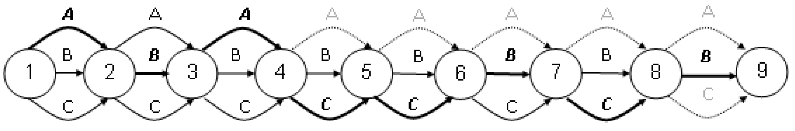
For example, there are three requirements, N = {A, B, C}, n = 3. Requirement A has two stages and requirements B and C each have three stages. Figure 2 shows the graph.
For example, an ant in the first step chose requirement A, then B, and again A. Requirement A has two stages, so the ant will ignore its remaining edges in the next steps (shown by the dotted line in Figure 3). Then, let the ant select requirements C, C, B, and C in succession, then only edge B remains valid at the 8th node. Because of the above pass, a sequence of requirements {A, B, A, C, C, B, C, B} will be obtained. Using this sequence, it is easy to obtain the stage selection sequence vector:
L** = {l1A, l1B, l2A, l1C, l2C, l2B, l3C, l3B}.
Figure 3 shows the path of the ant along the graph for this example. The selected edges are shown with thicker lines. The dotted line shows the edges that were ignored by the particle based on the selections made.
Thus, the problem under consideration differs from the weighted undirected graph traversal problem. However, to adapt the algorithm to these conditions, it is enough to place the leftmost vertex in the list of vertices of the graph that are allowed to start the bypass. The graph is not weighted; this is equivalent to the unit weight of all graph edges.
This approach to graph representation is universal, as it allows for considering various additional requirements. For example, in the classical formulation of the JSS problem, there are no dependencies between different stages of different jobs (all jobs are independent). For the proposed approach, it is easy to take into account such a modification of the problem. In addition, it becomes possible to solve scheduling problems that dynamically change. For example, when, after the plan is drawn up and the execution begins, the order of stages or the duration of stages change, or new works appear.
A more formalized description of the algorithm is given in Algorithms 1 and 2. Algorithm 1 presents the algorithm in general; Algorithm 2 shows the traversal of the graph by one ant.
| Algorithm 1. Pseudocode for the ACO Algorithm Application for JSS Problem | |
| Input: N, M, Iaco, Cant, fmin, fmax, α, β, γ, ρ, λ Output:T, makespan Auxiliary Variables: f, Cs, routes, makespans, best_route, best_makespan Initialization:Cs = Count_stages(N), f = I[n × Cs] ∙ fmin, best_makespan = ∞ Begin ACO-JSS Algorithm | |
| 1 2 3 4 5 6 7 8 9 10 11 12 13 14 15 16 17 18 19 20 21 22 23 24 25 26 | for (i = 1, …, Iaco) do for (a = 1, …, Cant) do makespanesa, routesa = Ant_route(N, M, Cs, f, α, β) end for for (a = 1, …, Cant) do for (s = 1, …, Cs) do j = routesa,s fs, j = fs,j + (γ/makespanesa)β end for end for a = argmina(makespanesa) if (makespanesa < best_makespan) then best_makespan = makespanesa best_route = routesa end if for (s = 1, …, Cs) do j = best_routes fs,j = λ∙fs,j end for for (φ ∈ f) do φ = max(min(φ∙(1 − ρ), fmax), fmin) end for end for T = JSS(best_route) makespan = best_makespan return T, makespan |
| End ACO-JSS Algorithm | |
In Algorithm 1 the following designations are introduced: Iaco is the number of ACO algorithm iterations; Cant is the number of ants; Cs is the total number of all stages of all jobs; I[A × B] is an identity matrix A × B.
Each ant traverses the graph at each algorithm iteration (rows 2–4). After that, the application of the pheromone is performed in accordance with Equations (7) (rows 5–10), (9) (rows 11–19), and (8) (rows 20–22). The schedule obtained with the best-found route is the output result of the algorithm (rows 24–26).
| Algorithm 2. Pseudo Code for the Ant_route | |
| Input: N, M, Cs, α, f Output:makespan, route Auxiliary Variables:p, sp, tabu_list, stage_counters, stages Initialization:route = 0[Cs], tabu_list = {}, stage_counters = 0[n] stagesi = Count_stages(Ni), i = 1, …, n Begin Ant_route Algorithm | |
| 1 2 3 4 5 6 7 8 9 10 11 12 13 14 15 16 17 18 19 20 21 22 23 24 25 | for (s = 1, …, Cs) do sp = 0 for (j = 1, …, n) do if (j ∉ tabu_list) then pj = (fs,j)α sp = sp + pj else pj = 0 end if end for for (j = 1, …, n) do if (j ∉ tabu_list) then pj = pj/sp end if end for j = Roulette_Selection(p) routes = j stage_countersj + = 1 if (stage_countersj = stagesj) then tabu_list = tabu_list ∪ j end if end for T = JSS(route) makespan = max(T) return makespan, route |
| End Ant_route Algorithm | |
In Algorithm 2, the following designations are introduced: tabu_list is the list of job numbers for which all stages are added to the schedule; stage_counters is the vector of the counters of added stages for each job; stages is the vector of the number of stages in each job.
During the traversal, the ant at each step chooses an edge. Edge selection means job selection, as shown in Figure 2 and Figure 3. The next stage of the selected job will be added to the schedule with the start of execution as soon as possible. Edge selection probabilities are calculated according to Equation 6 (rows 3–15). The probabilistic choice is made using roulette wheel simulation (rows 16–17). If the selected stage is the last stage for the corresponding job, then the stages of this job can no longer be selected (rows 18–21).
2.2. Adaptive Selection of Algorithm Parameters
As noted in [26,27,33,34,40,43], the quality of the solutions obtained using the ACO algorithm strongly depends on the coefficients (parameters) used in it. In the above algorithm, such coefficients are α, β, γ, ρ, λ (Equations (6)–(9). Since each of the coefficients can take an infinite number of values, the question arises of choosing the coefficients that make it possible to obtain a solution that is closest to the optimal one. Selecting coefficients manually is inefficient because of the large range of their values and the lack of methods for their selection. In this study, it is proposed to select coefficients using their evolutionary selection. The most common method for implementing such a selection is a genetic algorithm.
Algorithm 3 presents the GA application for tuning ACO parameters.
| Algorithm 3. Pseudo Code for the ACO Algorithm with GA Adaptation | |
| Input: N, M, Ig, Cg, Iaco, Cant, fmin, fmax Output:T, makespan, α, β, γ, ρ, λ Auxiliary Variables: population, prob, fitnesses, best_parameters, best_fitness, Pm Initialization:population = I[Cg × 5] ∙ Random[Cg × 5], fitnesses = [], prob = 0[Cg] best_fitness = ∞, Pm = 0.05 Begin ACO-GA Algorithm | |
| 1 2 3 4 5 6 7 8 9 10 11 12 13 14 15 16 | for (i = 1, …, Ig) do for (g = 1, …, Cg) do α, β, γ, ρ, λ = Scale(populationg) T, makespane = ACO_JSS(N, M, Iaco, Cant, fmin, fmax, α, β, γ, ρ, λ) fitnessesg = makespane end for for (g = 1, …, Cg) do if (fitnessesg < best_fitness) do best_fitness = fitnessesg best_parameters = populationg end if end for next_population = population for (j = 1, …, Cg/2) do prob = 1/fitnesses a = Roulette_Selection(prob) |
| 17 18 19 20 21 22 23 24 25 26 27 28 29 30 31 | b = Roulette_Selection(prob) x = round(Random()∙4) next_ population2j–1 = populationa,1 … x ∥ populationb, x+1 … 5 next_ population2j = populationb, 1 … x ∥ populationa,x+1 … 5 end for for (j = 1, …, Cg) do if (Random() < Pm)do next_ populationj = Random [5] end if end for population = next_population end for α, β, γ, ρ, λ = Scale(best_parameters) T, makespane = ACO_JSS(N, M, Iaco, Cant, fmin, fmax, α, β, γ, ρ, λ) return T, makespan, α, β, γ, ρ, λ |
| End ACO-GA Algorithm | |
In Algorithm 3, the following designations are introduced: Ig—the number of GA iterations; Cg—the number of chromosomes; and population—the population of GA chromosomes.
The ACO parameters selection is carried out according to the scheme described below:
- Generation of a random initial state. The first generation is created from randomly selected solutions (chromosomes), where the parameters α, β, γ, ρ, λ are used as genes (initialization in Algorithm 3).
- Calculation of the coefficient of survival (fitness). Each solution (chromosome) is assigned a certain numerical value, depending on its proximity to the value of the fitness function (rows 2–12).
- Reproduction. Chromosomes with greater fitness are more likely to pass to offspring, roulette selection, and a single-point crossover operation is performed (rows 13–25).
- Mutation. If it is randomly determined that it is necessary to carry out a mutation, then the chromosome is changed to a new random chromosome (rows 21–31).
- If the specified number of iterations is completed, then the problem is solved. Otherwise, steps 2–4 are repeated.
The operation of the genetic algorithm is an iterative process until a stopping criterion is met, such as a number of generations. In this case, we consider the problem of continuous optimization:
where F(x) is the objective function to be minimized (in this work, it is the function calculated by Equation (5)), D is the search area, and x = {α, β, γ, ρ, λ}. The results of the implementation of the adaptive properties of the ACO algorithm are given below, in Section 3. In this work, a genetic algorithm with a single-point crossover of two parents, 95% crossover probability, and 10% mutation probability is used. During mutation, one randomly selected coefficient is changed to a random number in the allowable range.
2.3. Improving the Performance of the Software Implementation of the Algorithm
With the approach described above, the solution search time increases dramatically, since the solution of the problem by the ACO algorithm is launched many times. The search speed can be significantly increased by parallelizing calculations by dividing the population into parts and distributing the computational load for working with these parts between processors.
The mutation and calculation of the fitness function of individuals can be easily parallelized since they occur independently for each individual. At the same time, data common to all individuals is used only for reading, so there are no difficulties with the need to synchronize these stages and waste time on blocking processes while waiting for resources to be released.
Crossover is more difficult to parallelize since during this stage there is an interaction between individuals from different parts of the population. However, there is no need for parallelization, since this stage takes negligible time compared to other calculations.
However, the higher the efficiency of parallelization, the higher the level at which it is performed. Since the ACO algorithm is stochastic, it seems reasonable to simply run multiple independent instances of the algorithm at the same time. Since this paper uses meta-optimization based on a genetic algorithm, then parallelization is performed at the level of calculating the GA fitness function. In Algorithm 3, row 4 occupies the vast majority of the running time of the entire algorithm and, at the same time, the loop in rows 2–6 is easily parallelized.
Since the algorithm requires multiple traversals of the graph and changing the pheromone on edges, the choice of the graph structure and the mechanism for applying the pheromone is very important. At first glance, it might seem that an implementation of a graph would be a set of nodes containing a list of edges, each of which contains a pointer to a neighboring node and quantitative characteristics (weight and amount of pheromone). However, the graph can be represented as a matrix of weights and a pheromone matrix. It is, first, easier to implement; second, lesser in terms of the amount of memory required (no need to store lists of pointers in each node); and, third, it works faster.
The following method is especially effective: apply the pheromone to the matrix representing the graph, not at the end of each iteration (after the graph has been traversed by all ants), but create a copy of the matrix and, after each ant has traversed, increase the value of the pheromone in this copy, and after the traversal stage is over, perform a reverse replacement.
Using this method (let us designate two pheromone graphs as fGraph and fTmpGraph) allows us to significantly increase the speed of calculations by applying the following trick. Within one iteration, the number of pheromones on each edge remains unchanged; therefore, the fkα values from Equation (6) also do not change within one iteration. In this case, there is no need to calculate them for each ant again. Then, at the initialization stage, the fTmpGraph edges receive the initial value of the pheromone, and the fGraph edges receive the initial value to the power of α. At each iteration, the ants, bypassing the graph, are guided by fGraph (it is no longer necessary to calculate fkα—it is the essence of increasing the speed), and the pheromone is deposited on fTmpGraph. After all the ants traverse the graph and the pheromone evaporates from the graph fTmpGraph, each k-th branch of fGraph receives a pheromone value equal to fTmpGraphk = (fTmpGraphk)α.
Equation (6) contains the operations of exponentiation. Depending on the compiler, raising a number to the power of e and calculating the natural logarithm may be faster than raising a number to an arbitrary power, so in the first case, the operation fα should be replaced as follows: fα = eαln(f). It should be noted that there are ways to quickly calculate the exponent and the natural logarithm. If there is a high probability that the coefficient α will be an integer, especially 1 or 2, then for this case it is possible to add a variant of the algorithm in which multiplication will replace the exponentiation functions.
3. Results and Discussion
The software implementation of the proposed algorithm has been tested on the well-known model JSS problems from [48,49,50] and the real-life manufacturing problems from [51]. Table 1 shows the values of the ACO algorithm’s coefficients, which were selected by the GA as the best for test tasks.
In Table 1 and the next two tables, the following designations are introduced:
- Iz is the number of runs over which averaging was carried out (with the same coefficients);
- Lmin is the best-obtained solution;
- Lavg is the solution averaged over Iz launches;
- Iaco is the number of ACO iterations;
- Cant is the number of ants;
- α is the degree of significance of the pheromone when choosing the graph edge (Equation (6));
- β is the non-linear pheromone deposition coefficient (Equation (7));
- ρ is the pheromone evaporation coefficient (Equation (8));
- γ is the linear coefficient of pheromone application (Equation (7));
- λ is the accounting factor for the best current solution (Equation (9)).
It follows from the data obtained that the best-found sets of coefficients differ even when solving the same problem. The search for the relationship between the coefficients and their correlation is a direction for further research.
The experiments showed a significant improvement in the results compared to those obtained earlier without the evolutionary selection of coefficients (best and average results were determined by 40 runs), which is reflected in Table 2.
In Table 2, in addition to those already described, the following notations are used:
- Lm1 is the best solution that was recorded before using the GA (the coefficients were selected manually);
- La1 is the average value of the solutions that were recorded before using the GA;
- Lg is the best solution that was obtained using the GA;
- Lga is the average value of the solutions that were obtained using the coefficients found by the GA;
- Lm2 is the best solution that was obtained using the coefficients found by averaging over other solved problems;
- La2 is the average value of the solutions that were obtained using the coefficients found by averaging over other solved problems (except for the coefficient γ).
Here, averaged coefficients are understood as a set of coefficients found as the arithmetic means among the best-found coefficients for problems of similar dimensions.
To assess the improvement in the quality of schedules compiled with the adaptation of the method parameters, quasi-optimal solutions to test problems were used [52]. The results are shown in Table 3. For the problem of processing plates, the result 657.55 [51] is given, which also coincides with the solution obtained in this paper.
The experiments showed a significant improvement in the results (up to 12%) compared to those found earlier (without the adaptation of the coefficients).
The solutions obtained by the proposed adaptive algorithm for many problems from [47,48,49] turned out to be no worse than the known quasi-optimal solutions for these problems. The deviation from the known quasi-optimal solutions does not exceed 6% (in the work of the founders of the ACO algorithm [27], they state the 10% deviation in their results to job-shop problems). At the same time, the adaptive method makes it possible to obtain guaranteed solutions of the specified quality at each run with enough iterations.
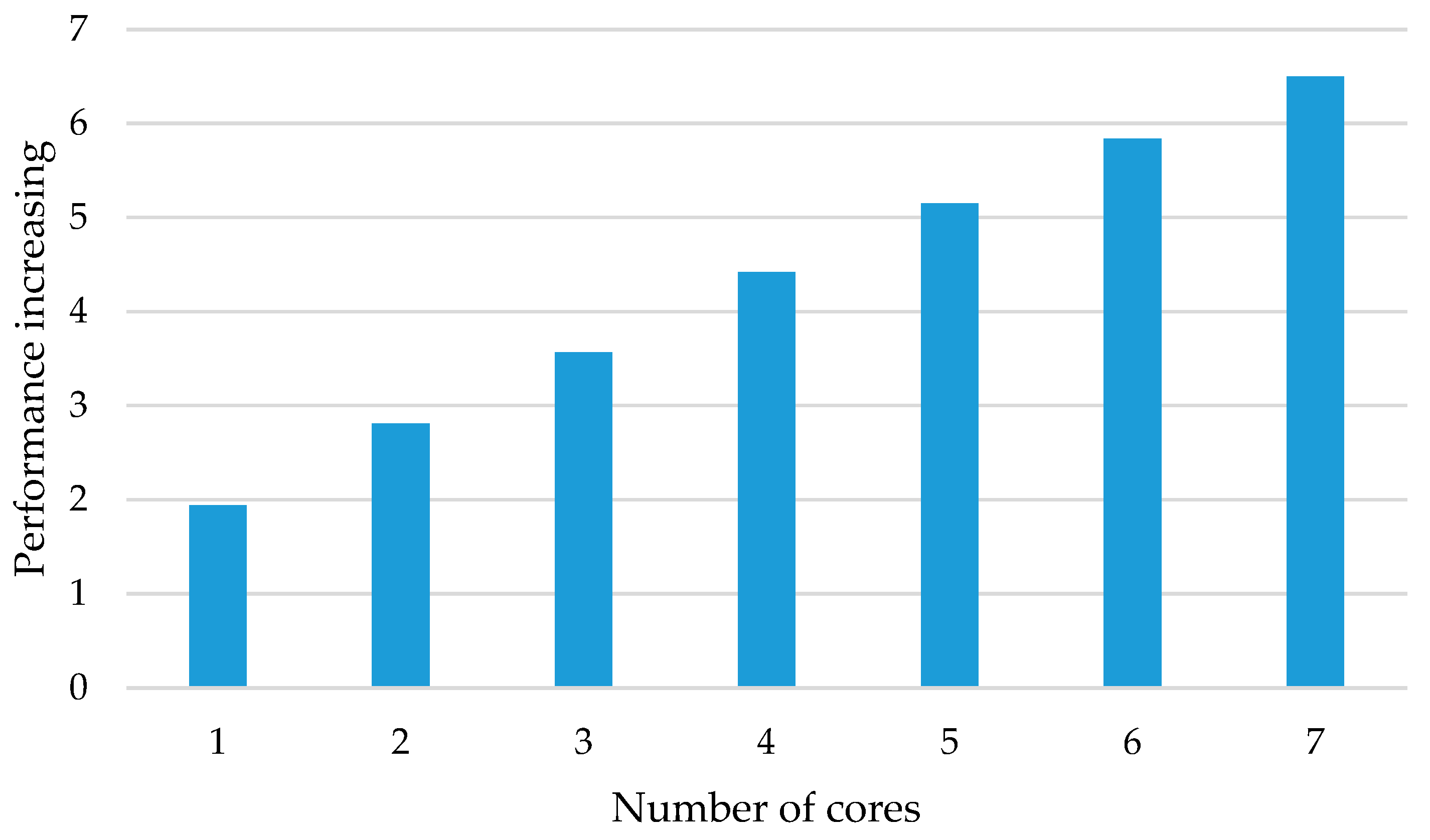
Figure 4 shows experimental data on the increase in the speed of parallel calculations compared to sequential operation, depending on the number of processors (cores) used.
It can be seen from the figure that the proposed approach can significantly reduce the computation time. The greater the effect of parallelization, the greater the number of calculations in solving the problem by the ACO algorithm, i.e., the greater the dimension of the problem, the number of ants, and the number of iterations. Indeed, according to Amdahl’s law, parallel computing is more effective the greater the proportion of calculations performed in parallel. In the test examples under consideration, the proportion of such calculations was 3–5%.
The greater the gain from the above technique of using two graphs, the greater the number of ants and the size of the graph. In test tasks of scheduling with 10 requirements in five stages, the calculation time was reduced by about four times; in tasks with 10 requirements in 10 stages—five times; in tasks with 50 requirements in 10 stages—seven times.
4. Conclusions
This study considers ways to improve the speed, accuracy, and flexibility of the ant colony optimization algorithm for solving scheduling problems. A new way of representing the problem as a problem of finding the shortest path on a graph is proposed, which is distinguished by a high level of universality and flexibility. At the same time, its use allows for obtaining acceptable job-shop scheduling problem solutions. It is shown that the use of the Genetic Algorithm as a meta-optimizer for tuning the parameters of the ACO algorithm simplifies the study, makes the algorithm adaptive to the problem being solved, and improves the resulting plans. It is determined that the sets of the best parameters of the algorithm differ from task to task.
For the next steps, we plan to conduct a study on a larger basis of scheduling instances, while covering not only job-shop scheduling problems but also open-shop scheduling (OSS) problems and flexible JSS and OSS problems [6,41,53,54] and considering the advantages of the proposed approach for planning problems with dynamically changing conditions [54,55,56]. In addition, the study of dependencies between the properties of the scheduling problem, the best values of the parameters of the ACO algorithm, and the efficiency of the solutions will be continued.
Funding
The research funding from the Ministry of Science and Higher Education of the Russian Federation (Ural Federal University Program of Development within the Priority-2030 Program) is gratefully acknowledged.
Data Availability Statement
Not applicable.
Conflicts of Interest
The authors declare no conflict of interest.
References
- Johnson, S.M. Optimal two- and three-stage production schedules with setup times included. Nav. Res. Logist. Q. 1954, 1, 61–68. [Google Scholar] [CrossRef]
- Lawler, E.L.; Lenstra, J.K.; Rinnooy Kan, A.H.G.; Shmoys, D.B. Sequencing and Scheduling: Algorithms and Complexity; Technische Universiteit Eindhoven: Eindhoven, The Netherlands, 1989. [Google Scholar]
- Brucker, P.; Knust, S. Complex Scheduling; Springer: Berlin, Germany, 2012. [Google Scholar]
- Xie, J.; Gao, L.; Peng, K.; Li, X.; Li, H. Review on flexible job shop scheduling. IET Collab. Intell. Manuf. 2019, 1, 67–77. [Google Scholar] [CrossRef]
- Leusin, M.E.; Frazzon, E.M.; Uriona Maldonado, M.; Kück, M.; Freitag, M. Solving the Job-Shop Scheduling Problem in the Industry 4.0 Era. Technologies 2018, 6, 107. [Google Scholar] [CrossRef] [Green Version]
- Xiong, H.; Danni, S.S.; Hu, R.J. A survey of job shop scheduling problem: The types and models. Comput. Oper. Res. 2022, 142, 105731. [Google Scholar] [CrossRef]
- Gonçalves, J.F.; de Magalhães Mendes, J.J.; Resende, M.G. A hybrid genetic algorithm for the job shop scheduling problem. Eur. J. Oper. Res. 2005, 167, 77–95. [Google Scholar] [CrossRef] [Green Version]
- Gromicho, J.A.S.; Hoorn, J.J.; Timmer, G.T. Exponentially better than brute force: Solving the job-shop scheduling problem optimally by dynamic programming. Comput. Oper. Res. Arch. 2012, 39, 2968–2977. [Google Scholar] [CrossRef]
- Çaliş, B.; Bulkan, S. A research survey: Review of AI solution strategies of job shop scheduling problem. J. Intell. Manuf. 2015, 26, 961–973. [Google Scholar] [CrossRef]
- Matrenin, P.V.; Manusov, V.Z. The cyclic job-shop scheduling problem: The new subclass of the job-shop problem and applying the simulated annealing to solve it. In Proceedings of the IEEE 2nd International Conference on Industrial Engineering, Applications and Manufacturing (ICIEAM), Chelyabinsk, Russia, 19–20 May 2022. [Google Scholar]
- Brucker, P.; Jurisch, B.; Sievers, B. A branch and bound algorithm for job shop scheduling problem. Discret. Appl. Math. 1994, 49, 107–127. [Google Scholar] [CrossRef] [Green Version]
- Baptiste, P.; Flamini, M.; Sourd, F. Lagrangian bounds for just-in-time job shop scheduling. Comput. Oper. Res. 2008, 35, 906–915. [Google Scholar] [CrossRef] [Green Version]
- Canbolat, Y.B.; Gundogar, E. Fuzzy priority rule for job shop scheduling. J. Intell. Manuf. 2004, 15, 527–533. [Google Scholar] [CrossRef]
- Klein, R. Bidirectional planning: Improving priority rule-based heuristic for scheduling resource-constrained projects. Eur. J. Oper. Res. 2000, 127, 619–638. [Google Scholar] [CrossRef]
- Stastny, J.; Skorpil, V.; Balogh, Z.; Klein, R. Job Shop Scheduling Problem Optimization by Means of Graph-Based Algorithm. Appl. Sci. 2021, 11, 1921. [Google Scholar] [CrossRef]
- Ziaee, M.; Mortazavi, J.; Amra, M. Flexible job shop scheduling problem considering machine and order acceptance, transportation costs, and setup times. Soft Comput. 2022, 26, 3527–3543. [Google Scholar] [CrossRef]
- Asadzadeh, L. A local search genetic algorithm for the job shop scheduling problem with intelligent agents. Comput. Ind. Eng. 2015, 85, 376–383. [Google Scholar] [CrossRef]
- Kundakcı, N.; Kulak, O. Hybrid genetic algorithms for minimizing makespan in dynamic job shop scheduling problem. Comput. Ind. Eng. 2016, 96, 31–51. [Google Scholar] [CrossRef]
- Gao, J.; Gen, M.; Sun, L.Y. A hybrid of genetic algorithm and bottleneck shifting for multiobjective flexible job shop scheduling problems. Comput. Ind. Eng. 2007, 53, 149–162. [Google Scholar] [CrossRef]
- Matrenin, P.V.; Sekaev, V.G. Particle Swarm optimization with velocity restriction and evolutionary parameters selection for scheduling problem. In Proceedings of the IEEE International Siberian Conference on Control and Communications (SIBCON), Omsk, Russia, 21–23 May 2015. [Google Scholar]
- Liu, B.; Wang, L.; Jin, Y.H. An effective hybrid PSO-based algorithm for flow shop scheduling with limited buffers. Comput. Oper. Res. 2008, 35, 2791–2806. [Google Scholar] [CrossRef] [Green Version]
- Xiang, W.; Lee, H.P. Ant colony intelligence in multi-agent dynamic manufacturing scheduling. Eng. Appl. Artif. Intell. 2008, 21, 73–85. [Google Scholar] [CrossRef]
- Matrenin, P.; Myasnichenko, V.; Sdobnyakov, N.; Sokolov, S.; Fidanova, S.; Kirillov, L.; Mikhov, R. Generalized swarm intelligence algorithms with domain-specific heuristics. IAES Int. J. Artif. Intell. 2021, 10, 157–165. [Google Scholar] [CrossRef]
- Zhang, C.Y.; Li, P.G.; Rao, Y.Q. A very fast TS/SA algorithm for the job shop scheduling problem. Comput. Oper. Res. 2008, 35, 82–294. [Google Scholar] [CrossRef]
- Wolpert, D.H.; Macready, W.G. No free lunch theorems for optimization. IEEE Trans. Evol. Comput. 1997, 1, 67–82. [Google Scholar] [CrossRef] [Green Version]
- Dorigo, M.; Blum, C. Ant colony optimization theory: A survey. Theor. Comput. Sci. 2005, 344, 243–278. [Google Scholar] [CrossRef]
- Dorigo, M.; Stützle, T. Ant colony optimization: Overview and recent advances. In Handbook of Metaheuristics; Springer: Cham, Switzerland, 2019; pp. 311–351. [Google Scholar]
- Neroni, M. Ant Colony Optimization with Warm-Up. Algorithms 2021, 14, 295. [Google Scholar] [CrossRef]
- Xu, Q.; Zhang, L.; Yu, W. A Localization Method of Ant Colony Optimization in Nonuniform Space. Sensors 2022, 22, 7389. [Google Scholar] [CrossRef] [PubMed]
- Wu, Y.; Gong, M.; Ma, W.; Wang, S. High-order graph matching based on ant colony optimization. Neurocomputing 2019, 328, 97–104. [Google Scholar] [CrossRef]
- Al-Shourbaji, I.; Helian, N.; Sun, Y.; Alshathri, S.; Abd Elaziz, M. Boosting Ant Colony Optimization with Reptile Search Algorithm for Churn Prediction. Mathematics 2022, 10, 1031. [Google Scholar] [CrossRef]
- D’andreagiovanni, F.; Krolikowski, J.; Pulaj, J. A fast hybrid primal heuristic for multiband robust capacitated network design with multiple time periods. Appl. Soft Comput. 2015, 26, 497–507. [Google Scholar] [CrossRef] [Green Version]
- Li, S.; Wei, Y.; Liu, X.; Zhu, H.; Yu, Z. A New Fast Ant Colony Optimization Algorithm: The Saltatory Evolution Ant Colony Optimization Algorithm. Mathematics 2022, 10, 925. [Google Scholar] [CrossRef]
- Chen, X.; Dai, Y. Research on an Improved Ant Colony Algorithm Fusion with Genetic Algorithm for Route Planning. In Proceedings of the 4th IEEE Information Technology, Networking, Electronic and Automation Control Conference (ITNEC), Electr Network, Chongqing, China, 12–14 June 2020; pp. 1273–1278. [Google Scholar]
- Bauer, A.; Bullnheimer, B.; Richard, F.H.; Strauss, C. An Ant Colony Optimization Approach for the Single Machine Total Tardiness Problem. In Proceedings of the Congress on Evolutionary Computation-CEC99, Washington, DC, USA, 6–9 July 1999; pp. 1445–1450. [Google Scholar]
- M’Hallah, R.; Alhajraf, A. Ant colony systems for the single-machine total weighted earliness tardiness scheduling problem. J. Sched. 2016, 19, 191–205. [Google Scholar] [CrossRef]
- Purism, A.; Bello, R.; Trujillo, Y.; Nowe, A.Y.; Martínez, Y. Two-Stage ACO to Solve the Job Shop Scheduling Problem. In Proceedings of the 12th Iberoamericann Congress on Pattern Recognition (CIARP), Valparaiso, Chile, 13–16 November 2007; pp. 447–456. [Google Scholar]
- Chaouch, I.L.; Driss, O.B.; Ghedira, K. A Modified Ant Colony Optimization algorithm for the Distributed Job shop Scheduling Problem. Procedia Comput. Sci. 2017, 112, 296–305. [Google Scholar] [CrossRef]
- Eswaramurthy, V.; Tamilarasi, A. Hybridizing tabu search with ant colony optimization for solving job shop scheduling problems. Int. J. Adv. Manuf. Technol. 2009, 40, 1004–1015. [Google Scholar] [CrossRef]
- Tran, L.V.; Huynh, B.H.; Akhtar, H. Ant Colony Optimization Algorithm for Maintenance, Repair and Overhaul Scheduling Optimization in the Context of Industrie 4.0. Appl. Sci. 2019, 9, 4815. [Google Scholar] [CrossRef] [Green Version]
- Wang, L.; Cai, J.; Li, M.; Liu, Z. Flexible Job Shop Scheduling Problem Using an Improved Ant Colony Optimization. Sci. Program. 2017, 9016303. [Google Scholar] [CrossRef] [Green Version]
- Blum, C.; Sampels, M. An Ant Colony Optimization Algorithm for Shop Scheduling Problems. J. Math. Model. Algorithms 2004, 3, 285–308. [Google Scholar] [CrossRef]
- Da Silva, A.R. Solving the Job Shop Scheduling Problem with Ant Colony Optimization. Available online: https://arxiv.org/abs/2209.05284 (accessed on 20 November 2022).
- Blum, C.; Ermeev, A.; Zakharova, Y. Hybridizations of evolutionary algorithms with Large Neighborhood Search. Comput. Sci. Rev. 2022, 46, 100512. [Google Scholar] [CrossRef]
- Grosan, C.; Abraham, A. Hybrid Evolutionary Algorithms: Methodologies, Architectures, and Reviews. Stud. Comput. Intell. 2007, 75, 1–7. [Google Scholar]
- Bramm, A.M.; Khalyasmaa, A.I.; Eroshenko, S.A.; Matrenin, P.V.; Papkova, N.A.; Sekatski, D.A. Topology Optimization of the Network with Renewable Energy Sources Generation Based on a Modified Adapted Genetic Algorithm. Energ. Proc. CIS High. Educ. Inst. Power Eng. Assoc. 2022, 65, 341–354. [Google Scholar] [CrossRef]
- Sipper, M.; Fu, W.; Ahuja, K.; Moore, J. Investigating the parameter space of evolutionary algorithms. BioData Min. 2018, 11, 2. [Google Scholar] [CrossRef] [Green Version]
- Adams, J.; Balas, E.; Zawack, D. The shifting bottleneck procedure for job shop scheduling. Manag. Sci. 1991, 34, 391–401. [Google Scholar] [CrossRef]
- Fisher, H.; Thompson, G. Probabilistic Learning Combination of Local Job-Shop Scheduling Rules in Industrial Scheduling; Prentice-Hall: Englewood Cliffs, NJ, USA, 1963. [Google Scholar]
- Lawrence, S. Supplement to Resource Constrained Project Scheduling: An Experimental Investigation of Heuristic Scheduling Techniques; Tech. rep., GSIA; Carnegie Mellon University: Pittsburgh, PA, USA, 1984. [Google Scholar]
- Sekaev, V.G. Using algorithms for combining heuristics in constructing optimal schedules. Inf. Technol. 2009, 10, 61–64. [Google Scholar]
- Beasley, J.E. OR-Library: Distributing test problems by electronic mail. J. Oper. Res. Soc. 1990, 41, 1069–1072. [Google Scholar] [CrossRef]
- Ahmadian, M.M.; Khatami, M.; Salehipour, A.; Cheng, T.C.E. Four decades of research on the open-shop scheduling problem to minimize the makespan. Eur. J. Oper. Res. 2021, 295, 399–426. [Google Scholar] [CrossRef]
- Luo, S.; Zhang, L.; Fan, Y. Real-Time Scheduling for Dynamic Partial-No-Wait Multiobjective Flexible Job Shop by Deep Reinforcement Learning. IEEE Trans. Autom. Sci. Eng. 2022, 19, 3020–3038. [Google Scholar] [CrossRef]
- Romanov, A.M.; Romanov, M.P.; Manko, S.V.; Volkova, M.A.; Chiu, W.-Y.; Ma, H.-P.; Chiu, K.-Y. Modular Reconfigurable Robot Distributed Computing System for Tracking Multiple Objects. IEEE Syst. J. 2021, 15, 802–813. [Google Scholar] [CrossRef]
- Wan, Y.; Zuo, T.-Y.; Chen, L.; Tang, W.-C.; Chen, J. Efficiency-Oriented Production Scheduling Scheme: An Ant Colony System Method. IEEE Access 2020, 8, 19286–19296. [Google Scholar] [CrossRef]
Figure 1.
An example of a JSS problem solution (Gantt chart).

Figure 2.
The JSS graph for the proposed ACO application scheme.

Figure 3.
An example of passing through a graph.

Figure 4.
The parallelization effect.


Table 1.
Examples of the best sets of coefficients obtained using the genetic algorithm.
| Problem | Iz | Lmin | Lavg | Iaco | Cant | α | β | ρ | γ | λ |
|---|---|---|---|---|---|---|---|---|---|---|
| abz6 | 40 | 948 | 977.333 | 1000 | 100 | 0.63 | 2.0 | 0.696 | 28 | 1.3 |
| abz6 | 40 | 945 | 982.524 | 1000 | 100 | 1.1 | 1.0 | 0.499 | 900 | 1.3 |
| ft10 | 40 | 950 | 995.866 | 1000 | 100 | 0.63 | 1.2 | 0.7 | 1000 | 1.1 |
| ft10 | 20 | 951 | 1006.1 | 1000 | 50 | 0.3781 | 1.711 | 0.97 | 1108.7 | 2.277 |
| la17 | 20 | 784 | 805.4 | 1000 | 100 | 0.392 | 2.7701 | 0.2998 | 425.5387 | 1.9615 |
| la17 | 20 | 785 | 798.25 | 1000 | 100 | 0.0341 | 1.7968 | 0.5461 | 949.1535 | 4.5589 |
| la15 | 20 | 1207 | 1215.45 | 1000 | 100 | 0.531 | 1.72 | 0.663 | 1032 | 1.2 |
| 3_Plates | 10 | 657.55 | 662.075 | 30 | 10 | 0.2782 | 0.4251 | 0.4919 | 296.61 | 2.5373 |
| 3_Plates | 10 | 657.55 | 662.3275 | 30 | 10 | 0.1754 | 0.5705 | 0.3836 | 326.05 | 2.5083 |
| la01 | 10 | 666 | 670.2 | 200 | 20 | 0.2262 | 0.8665 | 0.6883 | 903.3459 | 2.0363 |
| la01 | 10 | 666 | 669.4 | 200 | 20 | 0.3542 | 0.6527 | 0.8001 | 120.8012 | 2.1305 |
| la21 | 10 | 1107 | 1150.9 | 2000 | 100 | 0.7478 | 1.1134 | 0.3488 | 790.57 | 2.2236 |
| 6_Plates | 20 | 107 | 111.45 | 30 | 10 | 0.6218 | 2.7953 | 0.6995 | 335.6241 | 1.2376 |
| 6_Plates | 20 | 107 | 111.5 | 30 | 10 | 0.6204 | 0.2863 | 0.0775 | 137.6017 | 1.479 |
Table 2.
Examples of the best sets of coefficients obtained using the genetic algorithm.
| Problem | Lm1 | La1 | Lg | Lga | Lm2 | La2 | Iaco | Cant |
|---|---|---|---|---|---|---|---|---|
| abz6 | 980 | 1005.3 | 945 | 977.33 | 948 | 985.26 | 1000 | 100 |
| ft06 | 55 | 55.16 | 55 | 55 | 55 | 55.16 | 30 | 10 |
| ft10 | 1017 | 1038.8 | 950 | 995.87 | 975 | 1013.84 | 1000 | 100 |
| la01 | 666 | 673.08 | 666 | 669.4 | 666 | 673.08 | 30 | 10 |
| la10 | 958 | 958 | 958 | 958 | 958 | 958 | 1000 | 100 |
| la15 | 1211 | 1220.6 | 1207 | 1215.45 | 1207 | 1220.62 | 1000 | 100 |
| la17 | 796 | 809.32 | 784 | 798.25 | 787 | 809.32 | 1000 | 100 |
| la21 | 1121 | 1168.1 | 1107 | 1150.9 | 1118 | 1154.06 | 1000 | 100 |
| 3_Plates | 657.55 | 664.782 | 657.55 | 662.08 | 657.55 | 664.782 | 30 | 10 |
| 6_Plates | 109 | 113.22 | 107 | 111.45 | 108 | 112.12 | 30 | 10 |
Table 3.
Comparison of results.
| Problem | Lm1 | La1 | Lgm | Lga | Iaco | Cant | Best known |
|---|---|---|---|---|---|---|---|
| abz6 | 980 | 1005.3 | 945 | 977.33 | 1000 | 100 | 943 |
| ft06 | 55 | 55.16 | 55 | 55 | 30 | 10 | 55 |
| ft10 | 1017 | 1038.8 | 950 | 995.87 | 1000 | 100 | 930 |
| la01 | 666 | 673.08 | 666 | 669.4 | 30 | 10 | 666 |
| la10 | 958 | 958 | 958 | 958 | 1000 | 100 | 958 |
| la15 | 1211 | 1220.6 | 1207 | 1215.45 | 1000 | 100 | 1207 |
| la17 | 796 | 809.32 | 784 | 798.25 | 1000 | 100 | 784 |
| la21 | 1121 | 1168.1 | 1107 | 1150.9 | 1000 | 100 | 1048 |
| 3_Plates | 657.55 | 664.782 | 657.55 | 662.08 | 30 | 10 | 657.55 |
| 6_Plates | 109 | 113.22 | 107 | 111.45 | 30 | 10 | 107 |
Disclaimer/Publisher’s Note: The statements, opinions and data contained in all publications are solely those of the individual author(s) and contributor(s) and not of MDPI and/or the editor(s). MDPI and/or the editor(s) disclaim responsibility for any injury to people or property resulting from any ideas, methods, instructions or products referred to in the content. |
© 2022 by the author. Licensee MDPI, Basel, Switzerland. This article is an open access article distributed under the terms and conditions of the Creative Commons Attribution (CC BY) license (https://creativecommons.org/licenses/by/4.0/).
Share and Cite
MDPI and ACS Style
Matrenin, P.V. Improvement of Ant Colony Algorithm Performance for the Job-Shop Scheduling Problem Using Evolutionary Adaptation and Software Realization Heuristics. Algorithms 2023, 16, 15. https://doi.org/10.3390/a16010015
AMA Style
Matrenin PV. Improvement of Ant Colony Algorithm Performance for the Job-Shop Scheduling Problem Using Evolutionary Adaptation and Software Realization Heuristics. Algorithms. 2023; 16(1):15. https://doi.org/10.3390/a16010015
Chicago/Turabian StyleMatrenin, Pavel V. 2023. "Improvement of Ant Colony Algorithm Performance for the Job-Shop Scheduling Problem Using Evolutionary Adaptation and Software Realization Heuristics" Algorithms 16, no. 1: 15. https://doi.org/10.3390/a16010015
Note that from the first issue of 2016, this journal uses article numbers instead of page numbers. See further details here.