
A Lower Bound for the Query Phase of Contraction Hierarchies and Hub Labels and a Provably Optimal Instance-Based Schema †


Institut für Formale Methoden der Informatik, Universität Stuttgart, 70174 Stuttgart, Germany
*
Author to whom correspondence should be addressed.
†
This paper is an extended version of our paper published in Proceedings of the 15th International Computer Science Symposium in Russia, Ekaterinburg, Russia, 29 June–3 July 2020.
Algorithms 2021, 14(6), 164; https://doi.org/10.3390/a14060164
Submission received: 29 January 2021
/
Revised: 21 May 2021
/
Accepted: 22 May 2021
/
Published: 25 May 2021
(This article belongs to the Special Issue Selected Algorithmic Papers From CSR 2020)
Abstract
:We prove a lower bound on the query time for contraction hierarchies (CH) as well as hub labels, two popular speed-up techniques for shortest path routing. Our construction is based on a graph family not too far from subgraphs that occur in real-world road networks, in particular, it is planar and has a bounded degree. Additionally, we borrow ideas from our lower bound proof to come up with instance-based lower bounds for concrete road network instances of moderate size, reaching up to 96% of an upper bound given by a constructed CH. For a variant of our instance-based schema applied to some special graph classes, we can even show matching upper and lower bounds.
1. Introduction
While the problem of computing the shortest paths in general graphs with non-negative edge weights seems to have been well understood already decades ago, the last 10–15 years have seen tremendous progress when it comes to the specific problem of efficiently computing shortest paths in real-world road networks. Here, the idea is to spend some time for preprocessing where auxiliary information about the network is computed and stored, such that subsequent queries can be answered much faster than standard Dijkstra’s algorithm. One might classify most of the employed techniques into two classes: ones that are based on pruned graph search and others that are based on distance lookups. Most approaches fall into the former class, e.g., reach-based methods [1,2], highway hierarchies [3], arc-flags-based methods [4], or contraction hierarchies (CH) [5]. Here, Dijkstra’s algorithm is given a hand to ignore some vertices or edges during the graph search. The speed-up for road networks compared to plain Dijkstra’s algorithm ranges from one up to three orders of magnitude [1,5]. In practice, this means that a query on a country-sized network like that of Germany (~20 million nodes) can be answered in less than a millisecond compared to few seconds of Dijkstra’s algorithm. While these methods directly yield the actual shortest path, the latter class is primarily concerned with the computation of the (exact) distance between given source and target—recovering the actual path often requires some additional effort. Examples of such distance-lookup-based methods are transit nodes [6,7] and hub labels (HL) [8]. They allow for the answering of distance queries another one or two orders of magnitude faster.
There have also been attempts at theoretically explaining the impressive practical performance of these speed-up schemes. These approaches first identify certain properties of a graph, which supposedly characterize “typical” inputs in the real-world and then show that for graphs satisfying these properties, certain speed-up schemes have guaranteed query/construction time or space consumption. Examples of such graph characterizations are given via highway dimension [9], skeleton dimension [10], or bounded growth [11]. Note that these approaches are all concerned with upper bounds. For example, in [9] it is shown that for graphs with highway dimension h, after a preprocessing step, the number of considered nodes during a CH query is , which for polylogarithmic h is polylogarithmic in the network size. While small (i.e., constant or polylogarithmic) highway dimension is often assumed for real-world networks, note that even a simple grid has highway dimension , so the upper bound guaranteed by [9] is . Similarly, an analysis based on the bounded growth property [11] shows an upper bound of . In this work, we are concerned with two specific speed-up techniques: contraction hierarchies [5] and hub labels [8], and we provide lower bounds.
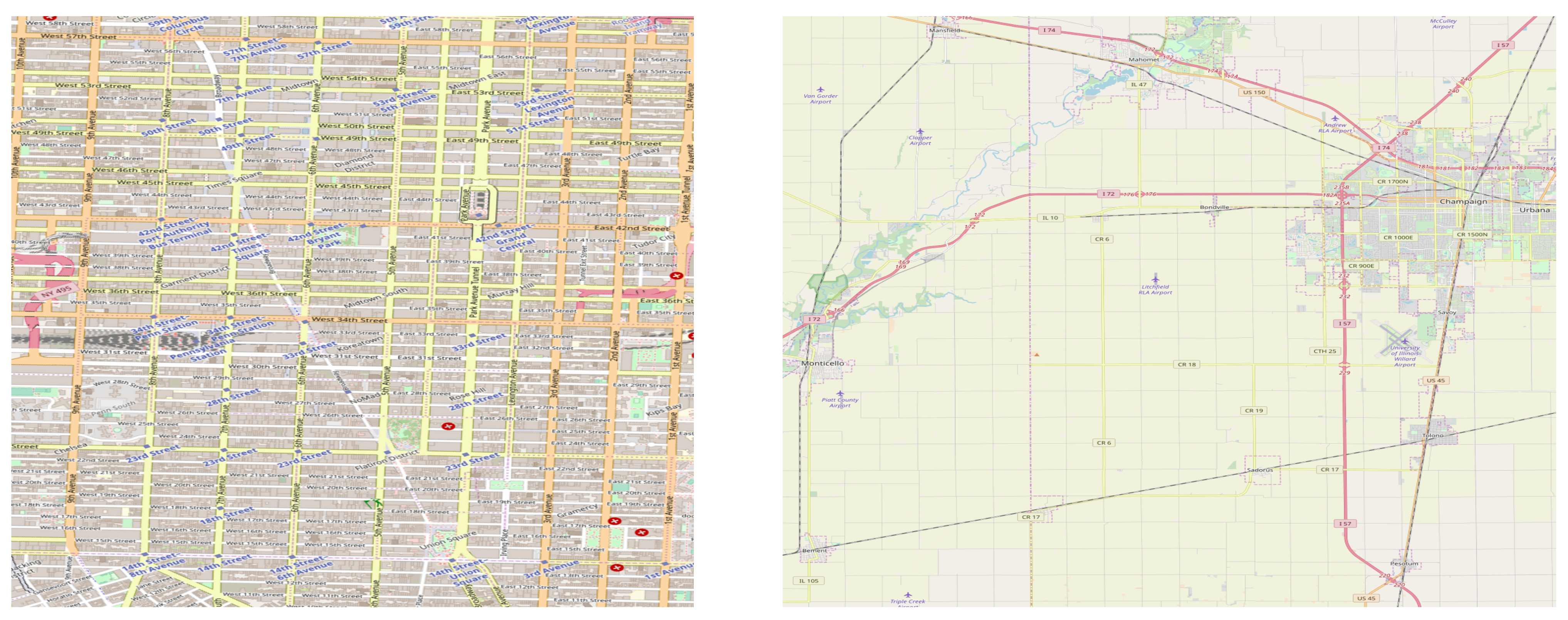
As grid-like substructures are quite common in real-world road networks (see Figure 1), one might ask whether better upper bounds for such networks are impossible in general or whether a polylogarithmic upper bound could be shown via more refined proof or CH construction techniques. Our work settles this question for contraction hierarchies as well as hub labels up to a logarithmic factor. We show that for CH, no matter what contraction order is chosen, and for HL, no matter how the hub labels are generated, there are grid networks for which not only the worst-case but even the average number of nodes to be considered during a query (which we call search space) is .
The insights of our theoretical lower bound analysis also allow us to devise a scheme to compute instance-based lower bounds, that is, for a given concrete road network, we algorithmically compute a lower bound on the average search space size. Note that such an instance-specific lower bound is typically much stronger than an analytical lower bound.
1.1. Related Work
In [9], a graph property called highway dimension is proposed to analyze the shortest path speed-up schemes. Intuitively, the highway dimension h of a graph is small if there exist sparse local hitting sets for shortest paths of a certain length. For contraction hierarchies and hub labels, a search space size of was proven (using a NP-hard preprocessing phase; polynomial time preprocessing increases this by a factor). While one might hope that real road networks exhibit a “small” highway dimension, e.g., constant or polylogarithmic, it is known that holds for grids. For hub labels, the so-called skeleton dimensionk [10] has been instrumented to prove a search space size of . Still, for grids, we have . In [12], CH were analyzed for graphs with treewidth t, and a query time of was shown. Yet, for grids we again have . Finally, the bounded growth model was introduced in [13], which also led to a search space size of for realistic graphs including grids. Specifically for planar graphs, the search space is by combining the planar separator Theorem [14] with nested dissection [12]. Therefore, our lower bound for the presented grid graph will be tight. In [15], White constructs for any given highway dimension h a family of graphs (as introduced in [16]) of highway dimension h, such that hub labeling requires a label size of and CH a query time of . Unfortunately, the graphs according to the author himself “are not representative of real-world graphs. For instance, the graphs do not have small separators and are not planar.” In fact, this could be more an indication of the unsuitability of the notion of highway dimension to characterize real-world road networks rather than a weakness of [15]. For transit nodes [7], instance-based lower bounds based on an LP formulation and its dual were derived in [17]. We are not aware of results regarding instance-based lower bound constructions for HL or CH.
1.2. Our Contribution and Outline
In this paper, we prove a lower bound on the search space (and hence the processing time) of the query phase of contraction hierarchies as well as hub labels. More concretely, we define so-called lightheaded grids for which we show that the average search space size is , irrespective of what contraction order or whatever hub labeling scheme was employed. Based on a grid, our graph is planar and has bounded degree. Our lower bound applies to CH [5] and HL [8] schemes. Based on our insights from the lower bound proof, we also show how to construct instance-based lower bounds algorithmically. Our experiments indicate that current CH constructions yield search space sizes close to optimal.
We first introduce basic properties of contraction hierarchies and hub labels and then present our main theoretical result. Then, we also show how to algorithmically construct instance-based lower bounds and present some experimental results. We conclude by proving that an instance-based schema of ours is optimal for ternary trees in the sense that it can yield tight lower bounds. Note that this paper is an extended version of a previous conference publication in [18]. Apart from a more elaborate exposition, we have added content with new insights and methods for computing instance-based lower bounds (Section 4.2.2 and Section 4.2.3), experimental evaluations for perturbed and lightheaded grids (Section 4.3), and a detailed analysis for which graph classes our lower bounding technique matches the upper bounds (Section 5).
2. Preliminaries
2.1. Contraction Hierarchies
The contraction hierarchies approach [5] computes an overlay graph in which so-called shortcut edges span large sections of shortest paths. This reduces the hop length of shortest paths and therefore allows a variant of Dijkstra’s algorithm to answer queries more efficiently.
The preprocessing is based on the so-called node contraction operation. Here, a node v as well as its adjacent edges are removed from the graph. In order not to affect shortest path distances between the remaining nodes, shortcut edges are inserted between two neighbors u and w of v, if and only if was a shortest path (which can easily be checked via a Dijkstra run). The cost of the new shortcut edge is the sum of costs of and . In the preprocessing phase, all nodes are contracted one-by-one in some order. The rank of the node in this contraction order is also called the level of the node.
Having contracted all nodes, the new graph contains all original edges of G as well as all shortcuts that were inserted in the contraction process. An edge —original or shortcut—is called upwards, if the level of v is smaller than the level of w, and downwards otherwise. By construction, the following property holds: For every pair of nodes , there exists a shortest path in that consists of a sequence of upward edges followed by a sequence of downward edges. This property allows us to search for the optimal path with a bidirectional Dijkstra only considering upwards edges in the search starting at s, and only downwards edges in the reverse search starting in t. This reduces the search space significantly and allows for answering of shortest path queries within the milliseconds range compared to seconds on a country-sized road network. We call this algorithm the CH-Dijkstra.
For our lower bound later on, the notion of direct search space (DSS) (as defined in [13]) is useful. A node w is in , if on the shortest path from v to w all nodes have level at most . Therefore, w will be settled with the correct distance in the CH-Dijkstra run. As a remark, the set of nodes considered during a CH-Dijkstra is usually a superset of as also nodes on monotonously increasing (w.r.t. level) but non-shortest paths are considered. Our construction will lower bound the size of which obviously also lower bounds the number of nodes that have to be considered during CH-Dijkstra.
2.2. Hub Labels
Hub labeling is a scheme to answer shortest path distance queries which differs fundamentally from graph search based methods. Here, the idea is to compute for every a label such that for given the distance between s and t can be determined by just inspecting the labels and . All the labels are determined in a preprocessing step (based on the graph G), later on, the graph G can even be discarded. There have been different approaches to compute such labels (even in theory); we will be concerned with hub labels that work well for road networks, following the ideas in [8]. To be more concrete, the labels we are interested in have the following form:
Here, we call a set of hubs—important nodes—for v. The hubs must be chosen such that for any , the shortest path from s to t intersects .
If such label sets are computed, the computation of the shortest path distance between s and t boils down to determining the node minimizing the summed distance. If the labels are stored lexicographically sorted, this can be done in a cache-efficient manner in time .
Knowing about CH, there is a natural way of computing such labels [8]: simply run an upward Dijkstra from each node v and let the label be the settled nodes with their respective distances. Clearly, this yields valid labels as CH answers queries exactly. The drawback is that the space requirement is quite large; depending on the metric and the CH construction, one can expect labels consisting of several hundreds to thousands node–distance pairs. It turns out, though, that many of the labels created in such a manner are useless as they do not represent shortest-path distance (as we restricted ourselves to a search in the upgraph only); pruning out those (which means reducing them to the direct search space of the respective node) typically reduces the label size by a factor of approximately 4. A source target distance query can then be answered in the microseconds range. This is not the only method to generate hub labels but our lower bound applies to any hub labeling scheme.
3. Theory: A Lower Bound Construction
In this section, we first provide a simple graph construction, which is essentially a slightly modified grid graph with some desirable properties. Then, we provide a lower bound on the direct search space size of any contraction order via an amortized analysis. A slight variation of the analysis also yields a lower bound for any hub labeling scheme. For the sake of simplicity, we assume without loss of generality that n is always a square number and a multiple of 4 for our analysis. Furthermore, our construction assumes an undirected graph, yet generalization to the directed case is quite straightforward.
3.1. The Lightheaded -Grid
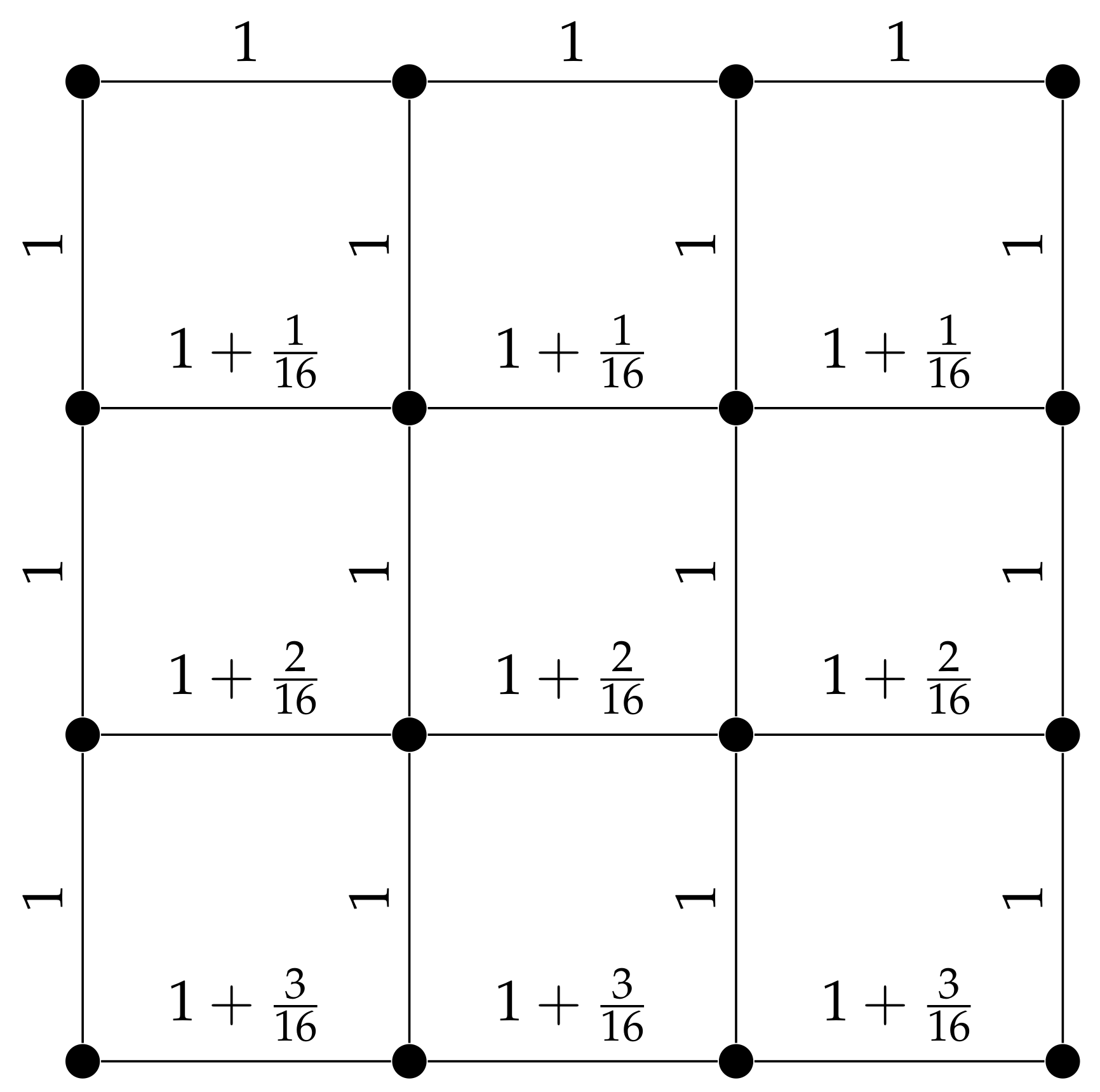
The basis of our construction is a regular grid with uniform edge costs. We then modify only costs of the horizontal edges such that they become ‘lighter towards the head’, thus the name lightheaded grid. More precisely, the horizontal edges in row i (, counted from top to bottom) have cost for some small enough . See Figure 2, for an example.
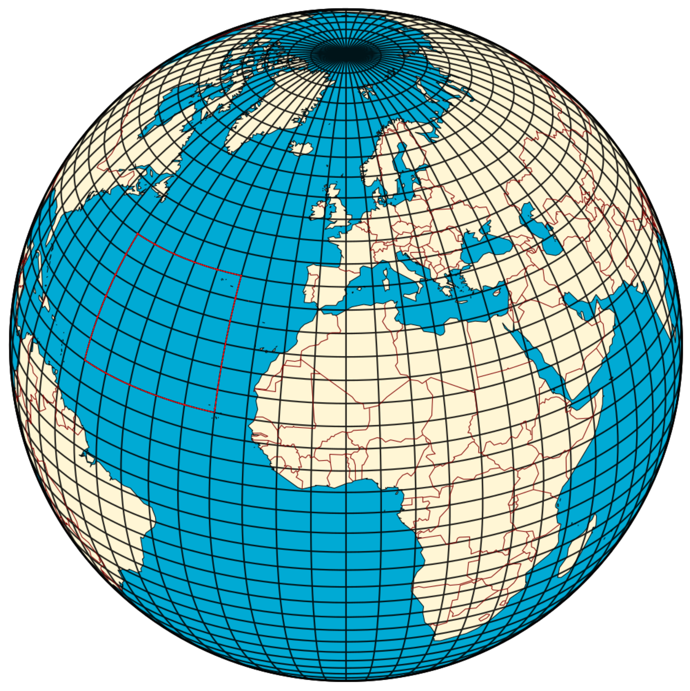
Note that the lightheaded grid structure can arise quite naturally in a real-world application: to route over large distances on the globe, a common approach is to discretize the planet along constant latitudes and longitudes, which can be seen in Figure 3, to build a graph upon the mentioned routing algorithms can operate. If source and target are both placed in the Northern Atlantic as indicated with the red axis-aligned rectangle, routing takes place on a light-headed grid.
3.2. Shortest Path Trees in Lightheaded Grids
For small enough choice of , the following Lemma holds:
Lemma 1.
For , the shortest path between some s and t in a lightheaded grid is unique and always consists of a horizontal and a vertical part, where the horizontal part is on the height of the higher of the nodes s and t.
Proof.
If a shortest path between s and t in the unweighted grid has cost d, the modified edge costs add a cost of less than 1 for the same path, thus all shortest paths in have (unweighted) Manhattan distance d. Let , where is the vertical and the horizontal distance. Any shortest Manhattan path must be composed of horizontal and vertical segments. In , horizontal edges towards the top have lower cost, thus the shortest path must have all its horizontal edges on the height of the higher of the nodes s and t. □
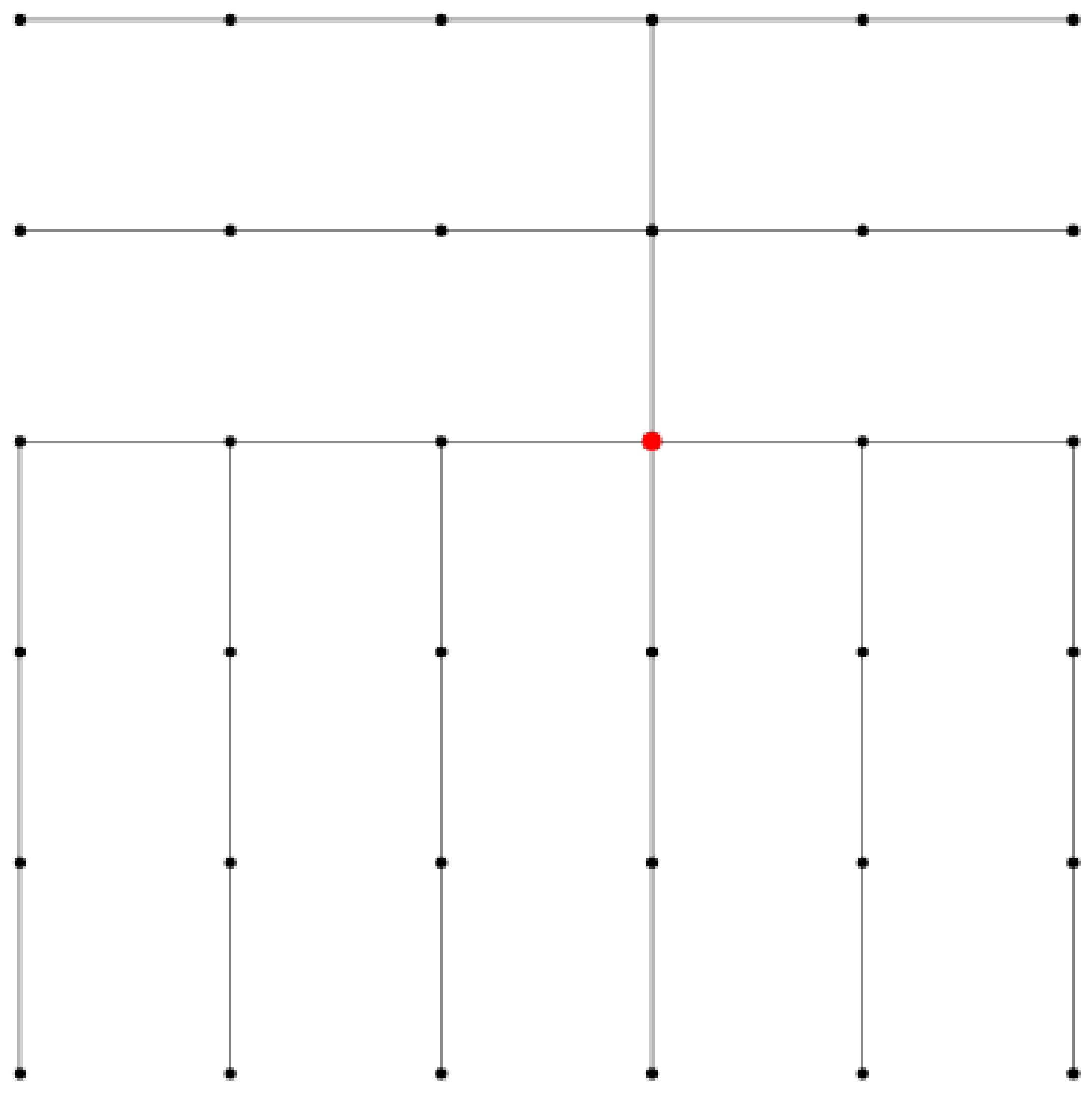
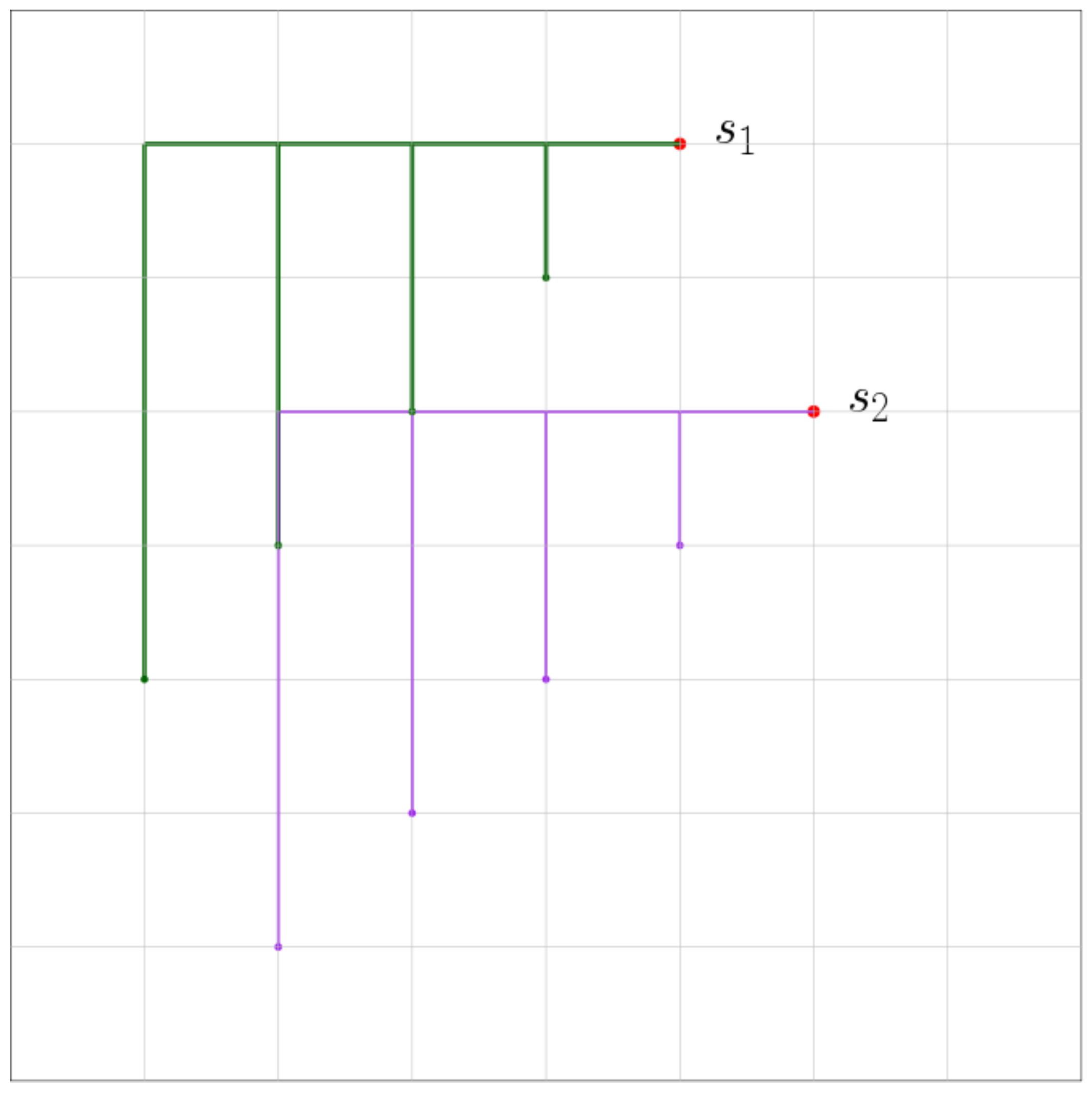
See Figure 4 for an illustration of a shortest path tree in the lightheaded grid. Observe that for all targets in the lower left and the upper right parts, the shortest path has an upper left corner, whereas for all targets in the upper left and lower right part, it has an upper right corner.
3.3. Lower Bounding the Direct Search Space
Let us now assume that the contraction hierarchy has been created with an arbitrary contraction order. We will show that no matter what this contraction order is, the average size of the direct search space is .
In our analysis, we only consider shortest path trees rooted in the top right quarter of the grid (there are of them). For these shortest path trees, their lower left part always contains a subtree of size as depicted in Figure 5.
The idea of the analysis is to identify pairs such that . We will consider each of the shortest path trees rooted at s in the top right quarter and for each identify such pairs (not necessarily with ). The main challenge will be to make sure that no double counting of pairs occurs when considering all these shortest path trees.
Let us focus on one shortest path tree rooted at s and the subtree of the lower left part as shown in Figure 6. By construction, we have vertical branches in this subtree.
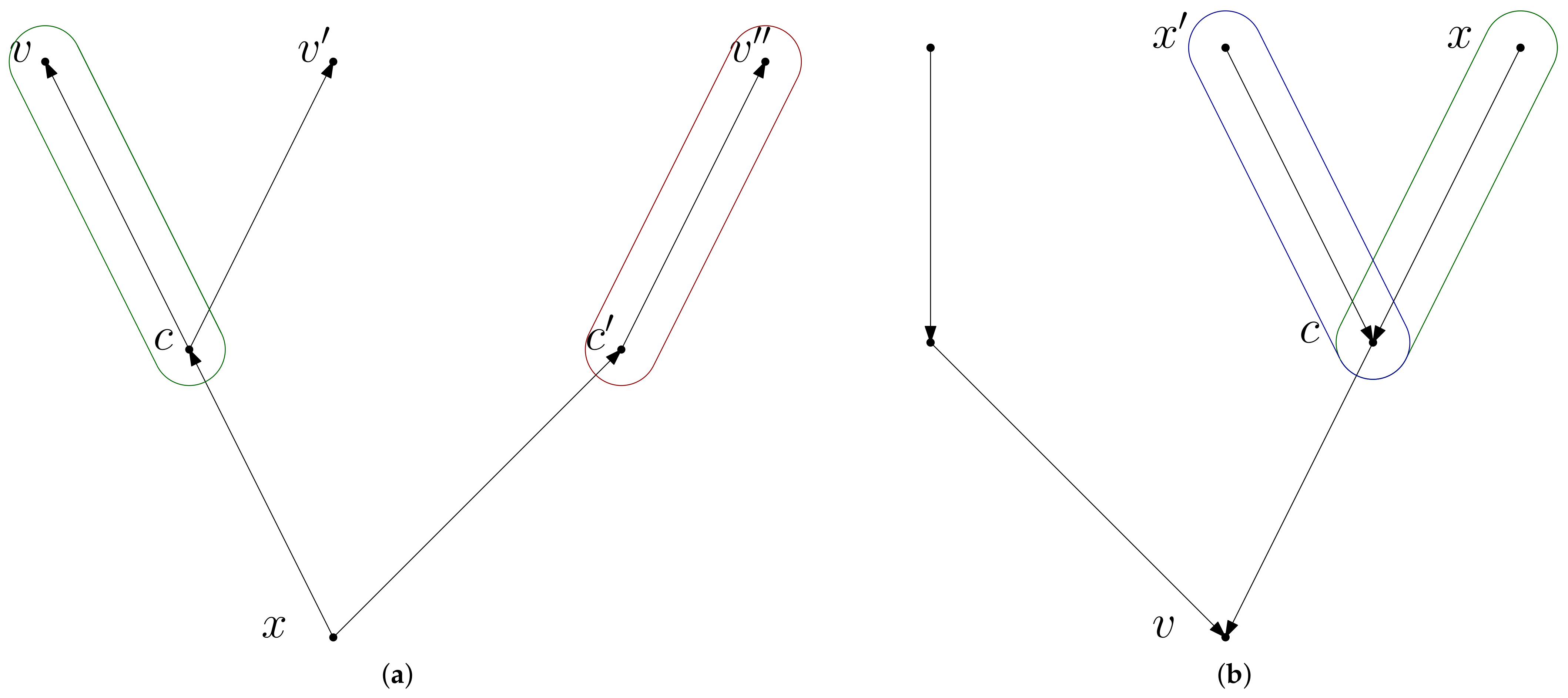
Consider one branch, spawning at its corner node c. Furthermore, let be the node in the branch which has the same distance to c as c to s. One can think of s being mirrored at c, see Figure 6. Let w be the highest-level node on the shortest path from s to . There are two cases: (a) w lies on the vertical branch including c (this is depicted as in Figure 6). (b) w lies on the horizontal part of the shortest path from s to excluding c (this is depicted as in the Figure). In case (a) we generate since obviously . In case (b), we cannot simply generate as the same pair might be identified when considering other branches in the shortest path tree from s leading to double counting. However, we also know that lies in the direct search space of . Intuitively, we charge by generating the pair .
Therefore, when considering the shortest path tree of a node s, we generate exactly one pair for each of the vertical branches to the lower left. Let us first show that we did not double count in this process.
Lemma 2.
No pair is generated more than once.
Proof.
Consider a pair that was generated according to case (a), i.e., s lies to the upper right or the right of v. Clearly, the same pair cannot be generated according to case (a) again, as the vertical branch in which v resides is only considered once from source s. However, it also cannot be generated according to case (b), as these pairs have always s to the lower left of v.
A pair generated according to case (b) has s to the lower left of v, thus cannot be generated by case (a) as these pairs have s to the upper right or right of v. As was generated according to case (b), it was generated when inspecting the shortest path tree from a source which is the node s mirrored at the corner vertex of the shortest path from s to v. However, this source is uniquely determined, so can only be generated when the shortest path tree rooted at with the vertical branch containing v was considered. □
Now, we are ready to prove the first main result of this paper.
Theorem 1.
The average direct search space of is .
Proof.
In our process, we considered shortest path trees, in each of which we identified pairs where and no pair appears twice. Therefore, we have identified such pairs, which on average yields . □
3.4. Lower Bounding of Hub Label Sizes
Note that the above argument and proof can be modified to also cover label sizes in a hub labeling scheme. Assume hub labels according to an arbitrary hub labeling scheme have been constructed. Then, when considering the shortest path tree rooted at s and the node in a vertical branch, we define w to be a node in . A pair corresponds to . Exactly the same arguments as above apply and we obtain the following second main result:
Theorem 2.
The average hub label size of is .
4. Practice: Instance-Based Lower Bounds
Our theoretical lower bound as just proven only applies to the lightheaded grid as defined before. Yet, even though similar substructures appear in real-world road networks, see Figure 1, the typical road network is certainly not a lightheaded grid and hence our lower bound proof does not apply.
Still, we can use the insights from the lower bound proof to construct instance-based lower bounds algorithmically. Concretely, for a given road network instance, we aim at computing a certificate which for this instance proves that the average search space size of a CH query, or the average hub label size cannot be below some lower bound, no matter what CH or HL construction was used.
Note that while for the previous lower bound proof we assumed an undirected graph for sake of a simpler exposition, we will now also include the more general case of a directed graph. To address the bidirectional nature of the CH-Dijkstra here we do now also have to differentiate between forward and backward search space. In the same vein, we refer to the forward and backward shortest path tree as and , respectively. Both the CH as well as the HL scheme can be easily generalized to directed graphs; in case of HL, compute for each node two labels, an outlabel storing distances fromv to hubs and an inlabel storing distances from hubs tov. A query from s to t is then answered by scanning the outlabel and the inlabel . CH also generalizes in a straightforward manner to the directed case, see in [5].
4.1. Witness Triples
In our lower bound proof for the lightheaded grid, we identified pairs such that , making use of a concrete (but arbitrary) CH (or HL) for the lightheaded grid to actually identify those pairs . We cannot do this for a given instance of a road network, since we would have to consider all possible CH/HL constructions. Therefore, instead of pairs let us now try to identify witness triples where c is again a node on the (directed) shortest path from x to v. The intuition for is the following: On the shortest path , some node of the suffix of must be in the forward search space of x, or some node on the prefix must be in the backward search space of v. This intuition mimics the proof idea in the previous section but also allowing for directed graphs and leaving the choice c open.
In the following, we sometimes treat paths just as sets of nodes to simplify presentation. Let us first define the notion of a conflict between two triples.
Definition 1 (conflict between triples)
We say two triples and are in conflict if at least one of the following conditions holds true:
- 1.
- and
- 2.
- and
See Figure 7a for a non-conflicting and Figure 7b for a conflicting example. Our goal will be to identify an as large as possible set W of conflict-free witness triples. The following Lemma proves that the size of such a set W lower bounds the average search space and label size.
Lemma 3.
If W is a set of conflict-free witness triples, then lower bounds the sum of (backward and forward) search spaces of all nodes in the network.
Proof.
Consider a triple and the following two cases:
- it accounts for a node in in the forward search space of x. Nodes in the forward search space of x can only be accounted for by triples . However, as due to W being conflict-free, we have not doubly accounted for it.
- it accounts for a node in in the backward search space of v. Nodes in the backwards search space of v can only be accounted for by triples . However, as due to W being conflict-free, we have not doubly accounted for it. □
For any witness set W, yields a lower bound on the average size of an in- or outlabel in case of the HL scheme, and on the average size of the direct search space from a single node in case of the CH scheme.
Therefore, it remains to compute a large conflict-free witness set W. Theoretically, one could enumerate all potential triples, build the conflict graph and use Integer Linear Programming (ILP) techniques to identify a conflict-free subset among the triples. A similar approach was conducted in [17] to compute lower bounds for transit nodes constructions. However, enumerating all potential triples in here seems somewhat inefficient (having to inspect such triples) on its own and employing the ILP techniques on top of it even more so. Therefore, in the following we propose a simple greedy heuristic. Again, let us emphasize that the resulting lower bound holds for any CH/HL construction for the given road network.
4.2. Generation of Witness Triples
In the following, we will describe two strategies for generating witness triples. The first method is based on an explicit representation of all shortest path trees with the advantage that the witness triple candidates are easily checked for conflict. The second method uses builds upon precomputed hub labels and requires little working space, yet requires extensive and non-trivial conflict checks of the triples. Therefore, we also devise a simple method to check for conflicts which does not require explicit path representations.
4.2.1. Method A: Fixed Lengths
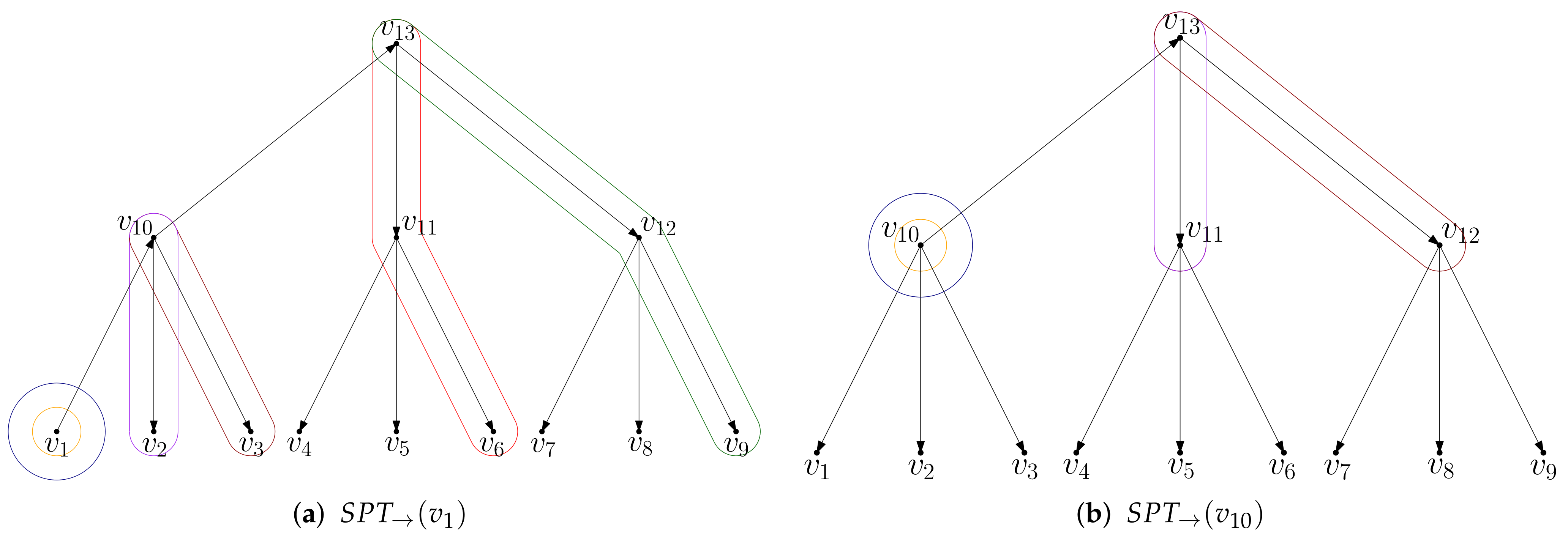
The high-level idea is as follows: We first compute and store all shortest path trees within the network (both forward and reverse). We then enumerate candidate shortest paths in increasing hop length (We define hop length as the number of nodes here). (always doubling and adding 1) from the shortest path trees, greedily adding corresponding triples to W in case no conflict is created. As center node c, we always choose the center node of a candidate path (in terms of hops), see, e.g., Figure 7a.
This specific choice for c as well as the decision to always roughly double the lengths of the considered candidate paths was motivated by the observation in practice that when considering a candidate triple , checking for conflict all triples and already present in W becomes quite expensive for large W. Intuitively, the latter decision ensures that triples with different hop lengths can never be in conflict at all, the former that not too many triples with the same source or target are generated.
Our actual greedy algorithm is stated in Algorithm 1. As we made sure that conflicts can only occur between triples with identical hop length, we can restrict the check for conflicts to the candidate set of triples of identical hop length. For an example of our greedy heuristic execution, look at the shortest path trees in Figure 7: Let us assume we collected the set of candidates for length 3 which contains , , , and beside other triples. We now pick the candidate and add it to W. Clearly, we remove this from our candidate set but we also have to remove because it would lead to a conflict in the forward shortest path tree and also remove because of the conflict in the backward tree .
Note that after computation of the shortest path trees, the collection of candidates can be organized in such a manner that each tree only needs to be traversed once. Moreover, the set of candidates can be subdivided over the shortest path trees and the center edges in buckets. As only candidates within one bucket need to be checked for conflicts, this leads to a reduced number of comparisons.
Storing and computing the shortest path trees require space and time when using Dijkstra’s algorithm (here, ). Generation and pruning of candidate triples can be bounded by , yet in practice the computation of the shortest path trees clearly dominates the running time.
4.2.2. Method B: Peak Nodes
Another strategy to generate witness triples uses on CH-based hub labels. Here, the idea is to enumerate triples with their center c being the highest-CH-level node on the shortest path from x to v. This approach is most efficiently implemented by enumerating via the the center c, i.e., determining all nodes x which have c in their outlabel and all nodes v which have c in their inlabel. If c is the highest-CH-level node on the shortest path , we have a valid triple candidate . Intuitively, high-CH-level nodes are “important” junctions in the road network and are hence a natural choice for center points occurring in many non-conflicting witness triples. The great advantage of this method is the modest space consumption which is essentially only the storage required for the hub labels. In contrast to the previous method, though, conflict checks of triples with coinciding source or target always have to be performed.
We want to emphasize that even though this construction method relies on precomputed hub labels, the resulting lower bound holds for any hub labeling scheme.
4.2.3. Efficient Conflict Check
Depending on the method for generating witness triple candidates, an efficient check for conflict is necessary. Our method A can already exclude many conflict tests, yet method B essentially has to check every candidate pair and . The following consideration allows for a fast evaluation of the test which does not require explicit path representations:
From (1) to (2) is basically Definition 1 for the case . If additionally , this is also implicitly covered. Furthermore, keep in mind that shortest paths are unambiguous. (2) is true if and only if there exists a common prefix of and , where c and are part of this prefix (3). In turn, this is equivalent that the c’s are part of the shortest paths of each other’s triple (4), which is only the case if the distance equations of (5) are fulfilled. The check for triples with coinciding targets proceed analogously. In practice, the distance lookups can be performed very quickly using a distance oracle like hub labels.
| Algorith 1 The algorithm to find a set of non-conflicting witness triples. |
| 1: procedure findWitnesses(G) 2: 3: 4: 5: while do 6: 7: while do 8: 9: 10: 11: pruneConflictingTriples 12: end while 13: 14: end while 15: return W 16: end procedure |
4.3. Experimental Results
We implemented our witness search heuristics in C++ and evaluated it on several graphs. Besides a very small test graph for sanity checking, we extracted real-world networks graphs based on Open Street Map (OSM) data for our main experiment. We picked Lower Manhattan to get a grid-like graph. For the street network of the German federal city-state Bremen, we created a large version car which includes all streets passable by car, as well as the versions fast car and highway only containing streets allowing at least a speed of 50 km/h and 130 km/h, respectively. The code was run on a 24-core Xeon(R) CPU E5-2650v4, 768 GB RAM machine.
To assess the quality of our lower bounds, we constructed a CH where the contraction order was defined by the so called edge-difference heuristic, that is, nodes that introduce few additional shortcuts are contracted first. This is one of the most popular contraction order heuristics. From this CH, we calculated the average (forward + backward) and compared it with the lower bounds computed by our two methods.
In Table 1, we list our results. Compared to our original paper [18], we realized that we can collect one more triple for every node due to a technicality which is described in more detail in Section 5.2. We updated the experiment results accordingly. Our biggest graph has over a quarter of a million edges and almost 120 k nodes. As expected, the space consumption is quadratic which makes our current algorithm infeasible for continental-sized networks. For the large Bremen graph, our 24-core machine took 32.5 h to complete the lower bound construction via our greedy heuristic and used 354 GB of RAM. Most important is the quotient which gives us a hint about the quality of our computed lower bound: For the highway version of Bremen, we achieve even , that is, the average search spaces in the computed CH are guaranteed to be less than a factor of above the optimum. Note, however, that this graph is atypical for road networks in the sense that it is far from being fully connected. The value of decreases for our bigger graphs down to around . The decrease can have several reasons: On one hand, our CH is based on a heuristic and is not necessarily optimal (no optimal algorithm is known), so even if we had brute-forced a maximum sized triple-set we would most certainly not achieve 100%. Indeed, our contribution is to show that the gap between the heuristic and the perfect is at most . On the other hand, the results strongly indicate that the missing of some long triples which do not have a length of becomes more relevant in bigger graphs. Note that it could also mean that the edge-difference heuristic performs worse on bigger graphs. It has been shown that constructing the optimal CH (even though according to a different optimality criterion) is NP-hard, see in [16], so we actually conjecture that finding the largest conflict-free set of triples would also turn out to be NP-hard if investigated further. Our alternative method B for generating witness triples consistently fares worse in terms of the constructed lower bound, but requires very little space. It remains to see whether a more elaborate order of considering witness candidates leads to better results, or if a different underlying contraction hierarchy (which determines in which order to enumerate the center points) makes a big difference.
In another experiment, we generated lightheaded grids graphs and tested them with our method A. The results can be seen in Table 2. According to expectations, the average search space is growing linearly with the side length of the grid. Fulfilling the intentions of its construction, the average search space of a lightheaded grid is quite high in comparison to real world grids: for a side length of 20, i.e., only 400 nodes in total, the search space size is close to the one of the much bigger real world graph bremen (car) with almost 120 k nodes. Furthermore, note that our approach for a trivial graph with only 1 node yields the tight bound. However, we also clearly see that the quality of the lower bound deteriorates with bigger grids. The reason is probably that the average search space size grows linearly with the side length of the grid but Method A is quite inflexible concerning triple length and therefore seems to collect only roughly triples.
As real street networks are not structured exactly like lightheaded grids but exhibit grid-like structures as seen in the introduction, we conducted a final experiment on grids with almost uniform weights, see Table 3. On one hand, slightly perturbed weights seem more realistic and on the hand, we need unique shortest paths for the computation anyway. Interestingly, we observe that both the size of the computed lower bounds as well as the average search space develop in less extreme manners than for the experiments on the lightheaded grid. Consequently, the term develops in similar way as for the real-world graphs. However, even though these perturbed grid graphs are not as awkward for the CH-heuristic to produce small average search spaces as their lightheaded counterparts, they still exhibit relatively big search spaces for a small number of nodes compared to our measured real-world networks.
Moreover, we coincidentally observed that sea-routing implementations based on a globe discretization as mentioned in Section 3.1 exhibited significantly underwhelming performance of the CH-technique when compared to its speedup on street networks of similar size. This confirms the relevance of Theorem 1.
5. Tightness of Instance-Based Lower Bounding Technique
In this last section, we want to investigate whether there are graph classes where our instance-based lower bounding techniques can yield lower bounds matching the upper bound. To that end we relax the conflict-free condition for the set W and show that this still yields a valid lower bound. This allows us to prove tight lower bounds for a some graph classes, the most interesting being balanced ternary trees. We also present other graph classes where our approach cannot deliver tight bounds.
5.1. Center-Conflict
Definition 2 (center-conflict)
For two conflicting triples and we say that they are
- forward center-conflicting if and
- backward center-conflicting if and
Intuitively, we say that triples are center-conflicting if the only reason for their conflict is the common center node.
Definition 3 (only-center-conflict)
We call a set only-center-conflictingif each triple has up to one forward and up to one backward center-conflict and is otherwise conflict-free.
Lemma 4.
A only-center-conflictingset still lower bounds the sum of search spaces of all nodes in the network.
Proof.
The argumentation builds up on Lemma 3. The difference is that if a node c is the highest node in both of two center-conflicting triples and , c seems to be doubly accounted in the forward search space of x. However, we can let account w.l.o.g. the triple for the node c in the forward search space of x and at the same time we do not have to let go away empty handed: We let account for the node c in the backward search space of . Now, it could happen that in the backward search space of there is a center-conflict of with another triple . Then, we let account for the node c in the forward search space of x and so on. Either this process terminates because there are no center-conflicts anymore or we come back to from where we started, but then we are done because already contributes to our search space. Therefore, each center-conflict can be resolved such that no double counting occurs. □
As a side note, we experimented with other triple definitions where, e.g., which can deliver as big sets W but we found the presented only-center-conflicting definition the easiest for the following analysis.
5.2. Special Triples Representing Nodes in Their Own Search Space
In the literature of analyzing search spaces, it is common that a node contributes to its own search space. Taking account of this with our triple definition forces us to do a minor technical adjustment: we allow triples of the form twice in our set, essentially making it a multiset. One can imagine there is one of these triples representing the forward search space and one for the backward search space. Other possibilities to handle that technical detail would be to not count nodes for their own search spaces or to assign a direction to triples, so that, e.g., and would be two distinguishable elements.
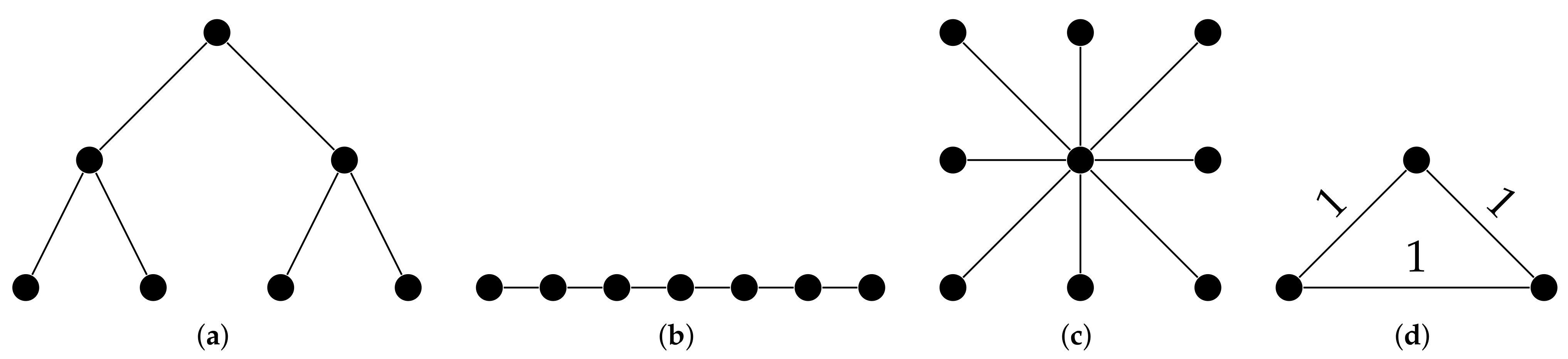
5.3. Balanced Ternary Trees
Lemma 5.
For a balanced ternary tree, a CH and an only-center-conflictingmultiset W can be found where and the average search space of the CH matches exactly.
Proof.
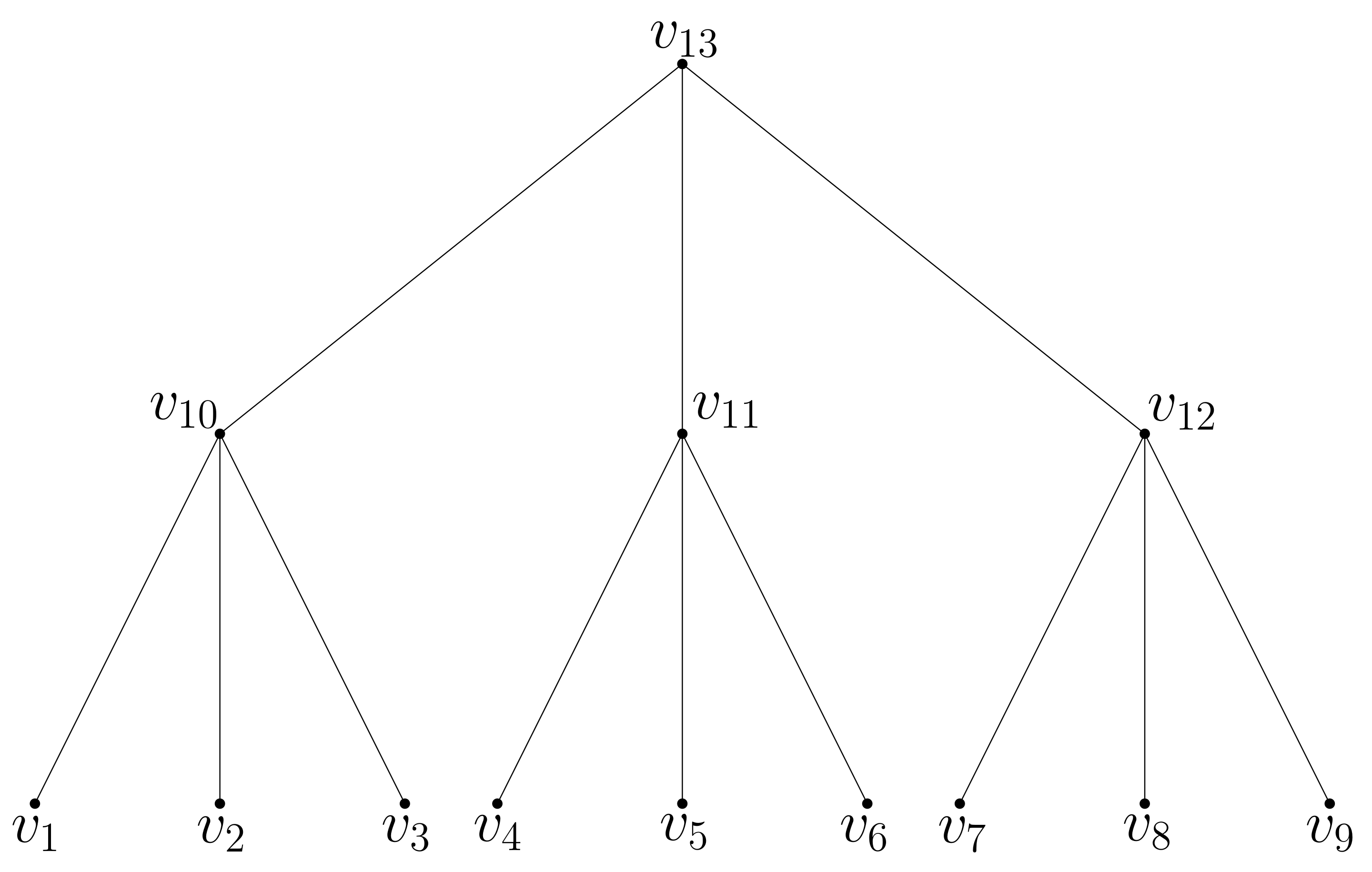
For an illustration of a balanced ternary tree see Figure 8, each undirected edge represents two directed edges, each for one direction.
We construct the CH in a natural way: Nodes closer to the root get higher levels and the root has the highest level. For the example in Figure 8, we chose the level equal to the node index. Then, the search space (forward or backward) of a node in the layer i, where is the layer of the root node, has size i. Let d be the depth of the tree, i.e., the number of layers, then the average search space (forward + backward) can be calculated as follows:
The factor 2 originates from putting forward and backward search space together, is for averaging, i nodes are in a search space of a node in depth i and we have nodes at depth i.
For the set , we choose the triples as illustrated in Figure 9.
In each shortest path tree, consider the path from the shortest path tree root s to the ternary tree root r. For each node c on such a path we can always find two triples of the form , where x has the same distance to c as s. Such triples can always be added without violating the conflict conditions. The two circles in the figure represent the special triples mentioned in Section 5.2. So for a node of layer i, triples appear in both of its forward and backward shortest path trees. As each triple appears in a forward and a backward tree, we have to divide the number of appearances by 2 at the end:
Therefore, . □
5.4. Balanced Binary Trees
Balanced binary trees seem to be the simplest graphs where our approach is unable to deliver tight lower bounds. For the balanced binary tree of depth 3 in Figure 10a, the straightforward (and almost certainly the optimal) contraction strategy from Section 5.3 yields
However, in contrast to finding non-conflicting triples for each node in the ternary tree, here we rather get only , because we only get the triples twice. This yields
and therefore . We can also easily see that this scheme leads to even worse coefficients for deeper balanced binary trees, i.e., .
5.5. Path Graph
For path graphs as depicted in Figure 10b, only allows a tight lower bound construction. For the straightforward contraction hierarchy can be constructed if the middle node gets the highest level and then the left and right parts get the level assigned in a recursive manner. Then the analysis becomes very similar to that of the balanced binary trees.
5.6. Star Graph
Star graphs like in Figure 10c allow tight lower bounds. The central node has to be the highest level and the triples can be chosen in a similar manner as for the balanced ternary tree so that they are center-conflicting only in the central node. Compared to the balanced ternary trees, there are much more possibilities for the choice of the triple set.
5.7. Balanced N-Ary Trees
For tight bounds can be computed, basically exactly like in the ternary tree case. Similar to the star graph case, there are more possibilities for the choice of triples.
5.8. Non-Tree Graphs
For non-tree graphs, the analysis becomes much more tedious as the SPT are not isomorphic to the original graph. Edge weights become also important as they define the SPTs, we focus on a simple triangle graph with uniform edge weights as in Figure 10d here. This triangle is symmetric in such a way that the contraction order can essentially be seen as unambiguous. It is easy to see that . Then, 4 triples can be set in each SPT in a straightforward and symmetric manner which yields , therefore the bound is tight here.
Of course, we expect more complicated non-trees to become non-tight quite easily as they are far more complex than tree graphs and even balanced binary tree graphs exhibit non-tightness. As a side note, in these examples the direct search space was equal to the actual search space which is in general not true for CHs on more complex non-tree graphs.
6. Materials and Methods
The code of method A for the experiments we described in Section 4.3 can be found under https://theogit.fmi.uni-stuttgart.de/ruppts/compchlowerbounds, accessed on 22 May 2021. There are also some of the smaller graphs included for reproducibility.
7. Conclusions
In this paper, we have proven a strong theoretical lower bound on the number of nodes that have to be considered during a CH search or HL lookup. Our lower bound instance is not too far from road network structures that occur in the real world. Our theoretical results imply that existing CH or HL construction schemes are essentially optimal (up to a logarithmic factor) for such grid-like networks.
In general, most theoretical considerations (in particular concerned with upper bounds) are somewhat unsatisfying in that they talk about the search space as the number of nodes that are visited in the search. In practice, the number of edges to relax is considerably larger than the number of nodes, though. Often, one simply upper bounds the number of edges by the square of the number of nodes to be considered (e.g., [9]), which is not really meaningful, if the latter is already . Furthermore, bounds not only on the direct search space but on the “real” search space during a CH query, i.e., including nodes that are considered with non-shortest-path distance, might be interesting to investigate.
More on the practical side, we instrumented the insights from our lower bound proof to come up with a construction scheme for instance-based lower bounds for CH and HL, if a concrete road network instance is given. For moderately sized networks, we could show that current CH and HL construction schemes indeed yield average search spaces not too far away from the optimum (less than a factor of 4). For a variant of our instance-based schema we have also shown that it can yield tight lower bounds for some graph classes, most notably ternary tree graphs. In future work, we aim at making the respective algorithms constructing the instance-based lower bounds more scalable to allow the lower bound construction even for country- or continent-sized networks. Furthermore, it might be worth investigating for which other graph classes our lower bounding technique has the potential to compute tight lower bounds. Perhaps it is even possible to slightly tweak our triple definition a step further to be potentially tight for every graph.
Author Contributions
Conceptualization, T.R. and S.F.; methodology, T.R.; software, T.R. and S.F.; validation, S.F.; formal analysis, T.R.; investigation, S.F.; resources, S.F.; data curation, T.R.; writing—original draft preparation, T.R. and S.F.; writing—review and editing, T.R. and S.F.; visualization, T.R. and S.F.; supervision, S.F.; project administration, S.F.; funding acquisition, S.F. Both authors have read and agreed to the published version of the manuscript.
Funding
This research received no external funding.
Data Availability Statement
Not applicable.
Acknowledgments
We like to thank the OpenStreetMap community for making free geodata available for our experiments.
Conflicts of Interest
The authors declare no conflict of interest.
Abbreviations
The following abbreviations are used in this manuscript:
| HL | Hub Label |
| CH | Contraction Hierarchy |
| DSS | Direct Search Space |
| SPT | Shortest Path Tree |
| OSM | Open Street Map |
References
- Gutman, R.J. Reach-Based Routing: A New Approach to Shortest Path Algorithms Optimized for Road Networks. In Proceedings of the Sixth Workshop on Algorithm Engineering and Experiments and the First Workshop on Analytic Algorithmics and Combinatorics, New Orleans, LA, USA, 10 January 2004; pp. 100–111. [Google Scholar]
- Goldberg, A.V.; Kaplan, H.; Werneck, R.F. Reach for A*: Efficient Point-to-Point Shortest Path Algorithms. In Proceedings of the Workshop on Algorithm Engineering and Experiments (ALENEX), Miami, FL, USA, 21 January 2006; pp. 129–143. [Google Scholar]
- Sanders, P.; Schultes, D. Engineering highway hierarchies. ACM J. Exp. Algorithmic 2012, 17. [Google Scholar] [CrossRef] [Green Version]
- Bauer, R.; Delling, D. SHARC: Fast and Robust Unidirectional Routing. In Proceedings of the Workshop on Algorithm Engineering and Experiments (ALENEX), San Francisco, CA, USA, 19 January 2008; pp. 13–26. [Google Scholar]
- Geisberger, R.; Sanders, P.; Schultes, D.; Vetter, C. Exact Routing in Large Road Networks Using Contraction Hierarchies. Transp. Sci. 2012, 46, 388–404. [Google Scholar] [CrossRef]
- Bast, H.; Funke, S.; Sanders, P.; Schultes, D. Fast routing in road networks with transit nodes. Science 2007, 316, 566. [Google Scholar] [CrossRef] [PubMed] [Green Version]
- Bast, H.; Funke, S.; Matijevic, D.; Sanders, P.; Schultes, D. In Transit to Constant Time Shortest-Path Queries in Road Networks. In Proceedings of the Workshop on Algorithm Engineering and Experiments (ALENEX), New Orleans, LA, USA, 6 January 2007. [Google Scholar]
- Abraham, I.; Delling, D.; Goldberg, A.V.; Werneck, R.F. Hierarchical Hub Labelings for Shortest Paths. In Lecture Notes in Computer Science; Springer: New York, NY, USA, 2012; Volume 7501, pp. 24–35. [Google Scholar]
- Abraham, I.; Fiat, A.; Goldberg, A.V.; Werneck, R.F. Highway Dimension, Shortest Paths, and Provably Efficient Algorithms. In Proceedings of the 21st Annual ACM-SIAM Symposium on Discrete Algorithms (SODA), Austin, TX, USA, 17–19 January 2010; pp. 782–793. [Google Scholar]
- Kosowski, A.; Viennot, L. Beyond Highway Dimension: Small Distance Labels Using Tree Skeletons. In Proceedings of the 28th Annual ACM-SIAM Symposium on Discrete Algorithms (SODA), Barcelona, Spain, 16–19 January 2017; pp. 1462–1478. [Google Scholar]
- Blum, J.; Funke, S.; Storandt, S. Sublinear Search Spaces for Shortest Path Planning in Grid and Road Networks. In Proceedings of the 32nd AAAI Conference on Artificial Intelligence (AAAI), New Orleans, LA, USA, 2–7 February 2018; pp. 6119–6126. [Google Scholar]
- Bauer, R.; Columbus, T.; Rutter, I.; Wagner, D. Search-Space Size in Contraction Hierarchies. In Proceedings of the 40th International Colloquium on Automata, Languages, and Programming (ICALP), Riga, Latvia, 8–12 July 2013; Volume 6124, pp. 93–104. [Google Scholar]
- Funke, S.; Storandt, S. Provable Efficiency of Contraction Hierarchies with Randomized Preprocessing. In Proceedings of the 26th International Symposium on Algorithms and Computation (ISAAC), Nagoya, Japan, 9–11 December 2015; Volume 9472, pp. 479–490. [Google Scholar]
- Lipton, R.J.; Tarjan, R.E. A separator theorem for planar graphs. SIAM J. Appl. Math. 1979, 36, 177–189. [Google Scholar] [CrossRef]
- White, C. Lower Bounds in the Preprocessing and Query Phases of Routing Algorithms. In Proceedings of the 23rd Annual European Symposium on Algorithms (ESA), Patras, Greece, 14–16 September 2015; pp. 1013–1024. [Google Scholar]
- Milosavljević, N. On optimal preprocessing for contraction hierarchies. In Proceedings of the 5th ACM SIGSPATIAL IWCTS, Redondo Beach, CA, USA, 23–25 November 2012; pp. 33–38. [Google Scholar]
- Eisner, J.; Funke, S. Transit Nodes-Lower Bounds and Refined Construction. In Proceedings of the 14th Workshop on Algorithm Engineering and Experiments (ALENEX), Kyoto, Japan, 16 January 2012; pp. 141–149. [Google Scholar]
- Rupp, T.; Funke, S. A lower bound for the query phase of contraction hierarchies and hub labels. In International Computer Science Symposium in Russia; Springer: New York, NY, USA, 2020; pp. 354–366. [Google Scholar]
Figure 1.
Grid-like substructures in real networks (Manhattan on the left, Urbana-Champaign on the right) (by OpenStreetMap).
Figure 1.
Grid-like substructures in real networks (Manhattan on the left, Urbana-Champaign on the right) (by OpenStreetMap).

Figure 2.
Lightheaded grid for .

Figure 3.
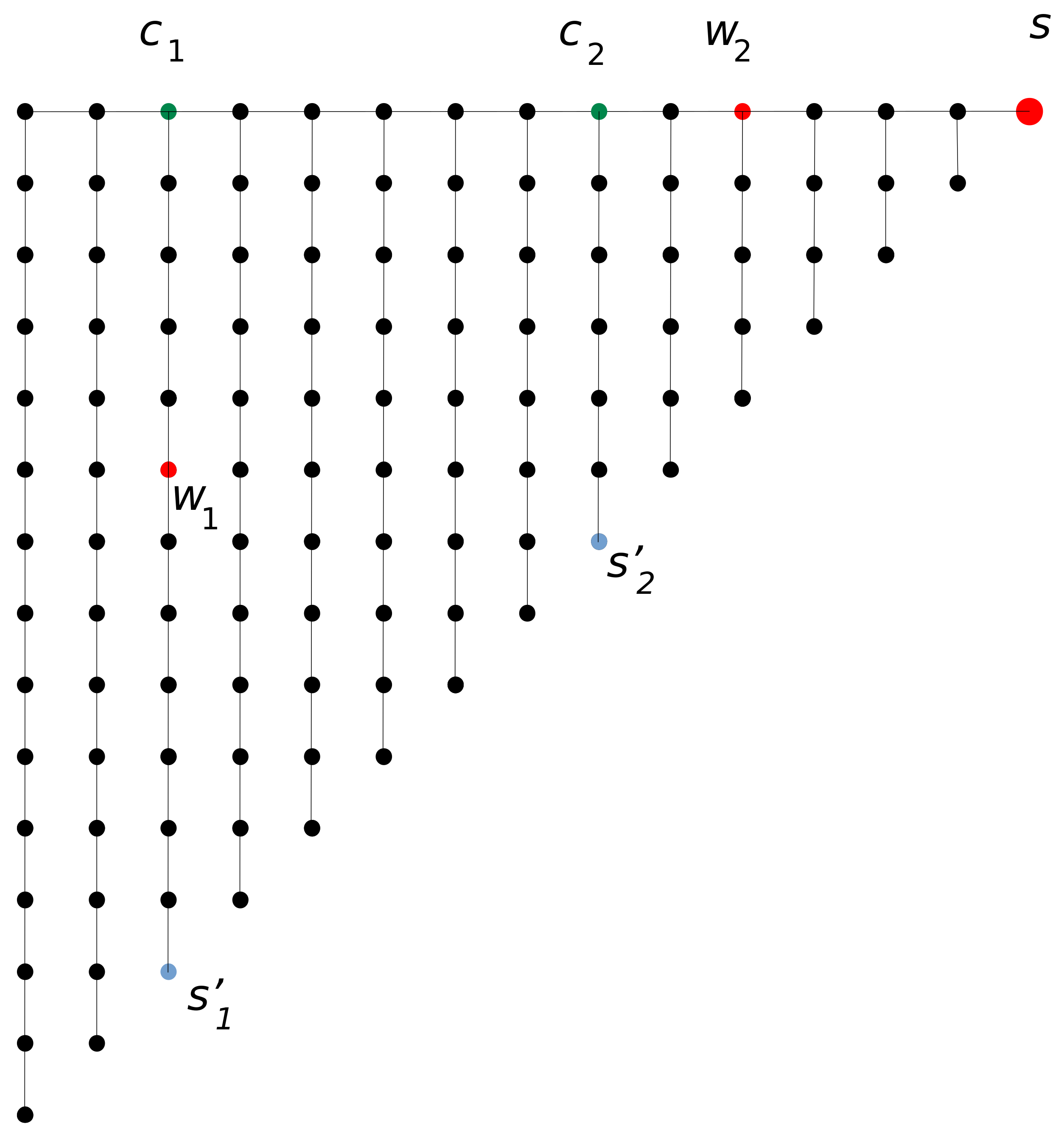
Light-headed grid appearing in discretization of the globe along constant latitudes and longitudes. (Based on a image by Hellerick-Own work, CC BY-SA 3.0, https://commons.wikimedia.org/w/index.php?curid=26737079, accessed on 22 May 2021).
Figure 3.
Light-headed grid appearing in discretization of the globe along constant latitudes and longitudes. (Based on a image by Hellerick-Own work, CC BY-SA 3.0, https://commons.wikimedia.org/w/index.php?curid=26737079, accessed on 22 May 2021).

Figure 4.
Shortest path tree from red source.

Figure 5.
Relevant lower left parts of shortest path trees rooted in top right quarter.

Figure 6.
Subtree in the lower left of a shortest path tree and charging argument.

Figure 7.
Examples for witness triples in shortest path trees. (a) Forward shortest path tree : The witness triple where the relevant nodes for the conflict check are in the green bubble. There is no conflict with and its relevant nodes in the red bubble; (b) : The green witness triple of the left Figure shown in the backward tree of v. It is in conflict with the blue triple because they share the node c.

Figure 8.
Balanced ternary tree.

Figure 9.
Shortest path trees.

Figure 10.
Example for Graphs. (a) Balanced binary tree; (b) Path graph; (c) Star graph; (d) Triangle graph.
Figure 10.
Example for Graphs. (a) Balanced binary tree; (b) Path graph; (c) Star graph; (d) Triangle graph.


Table 1.
Experimental results.
| Test Graph | Lower Manhattan | Bremen (Fast Car) | Bremen (Car) | Bremen (Highway) | |
|---|---|---|---|---|---|
| # nodes | 22 | 2828 | 40,426 | 119,989 | 1781 |
| # edges (org) | 52 | 4020 | 64,663 | 227,567 | 1766 |
| # edges (CH) | 77 | 7752 | 126,055 | 400,038 | 3340 |
| -construction space (A) | MB | 233 MB | 40 GB | 354 GB | 84 MB |
| -construction space (B) | MB | MB | 91 MB | 328 MB | 6 MB |
| -construction time (A) | <1 s | 36 s | 100 m | h | <1 s |
| -construction time (B) | <1 s | 10 s | 80 m | h | <1 s |
| (A) | |||||
| (B) | |||||
| (A) | |||||
| (B) |
Table 2.
Experimental results on light headed grid.
| Side Length | 1 | 5 | 10 | 15 | 20 | 25 |
|---|---|---|---|---|---|---|
Table 3.
Experimental results on grid with almost uniform weights.
| Side Length | 1 | 5 | 10 | 15 | 20 | 25 |
|---|---|---|---|---|---|---|
Publisher’s Note: MDPI stays neutral with regard to jurisdictional claims in published maps and institutional affiliations. |
© 2021 by the authors. Licensee MDPI, Basel, Switzerland. This article is an open access article distributed under the terms and conditions of the Creative Commons Attribution (CC BY) license (https://creativecommons.org/licenses/by/4.0/).
Share and Cite
MDPI and ACS Style
Rupp, T.; Funke, S. A Lower Bound for the Query Phase of Contraction Hierarchies and Hub Labels and a Provably Optimal Instance-Based Schema. Algorithms 2021, 14, 164. https://doi.org/10.3390/a14060164
AMA Style
Rupp T, Funke S. A Lower Bound for the Query Phase of Contraction Hierarchies and Hub Labels and a Provably Optimal Instance-Based Schema. Algorithms. 2021; 14(6):164. https://doi.org/10.3390/a14060164
Chicago/Turabian StyleRupp, Tobias, and Stefan Funke. 2021. "A Lower Bound for the Query Phase of Contraction Hierarchies and Hub Labels and a Provably Optimal Instance-Based Schema" Algorithms 14, no. 6: 164. https://doi.org/10.3390/a14060164
Note that from the first issue of 2016, this journal uses article numbers instead of page numbers. See further details here.