
Detection of Representative Variables in Complex Systems with Interpretable Rules Using Core-Clusters
by
 , and
, and
Camille Champion
1, 
Anne-Claire Brunet
1,
Rémy Burcelin
2,
Jean-Michel Loubes
1,3,* and
Laurent Risser
1,3 
1
Toulouse Mathematics Institute (UMR 5219), CNRS, University of Toulouse, F-31062 Toulouse, France
2
Institute of Cardiovascular and Metabolic Diseases INSERM, F-31432 Toulouse, France
3
Artificial and Natural Intelligence Toulouse Institute (3IA ANITI), F-31000 Toulouse, France
*
Author to whom correspondence should be addressed.
Algorithms 2021, 14(2), 66; https://doi.org/10.3390/a14020066
Submission received: 15 January 2021
/
Revised: 10 February 2021
/
Accepted: 12 February 2021
/
Published: 22 February 2021
(This article belongs to the Special Issue Interpretability, Accountability and Robustness in Machine Learning)
Abstract
:In this paper, we present a new framework dedicated to the robust detection of representative variables in high dimensional spaces with a potentially limited number of observations. Representative variables are selected by using an original regularization strategy: they are the center of specific variable clusters, denoted CORE-clusters, which respect fully interpretable constraints. Each CORE-cluster indeed contains more than a predefined amount of variables and each pair of its variables has a coherent behavior in the observed data. The key advantage of our regularization strategy is therefore that it only requires to tune two intuitive parameters: the minimal dimension of the CORE-clusters and the minimum level of similarity which gathers their variables. Interpreting the role played by a selected representative variable is additionally obvious as it has a similar observed behaviour as a controlled number of other variables. After introducing and justifying this variable selection formalism, we propose two algorithmic strategies to detect the CORE-clusters, one of them scaling particularly well to high-dimensional data. Results obtained on synthetic as well as real data are finally presented.
1. Introduction
Discovering representative variables in high dimensional and complex systems with a limited number of observations is a recurrent problem of machine learning. Heterogeneity between the variables behavior and multiple similarities between variable subsets often make this process ambiguous. A convenient strategy to solve this task is to associate each representative variable of the complex system to a cluster of variables, and to model the relations between variables in a graph [1]. The complex systems are indeed typically modeled as undirected weighted graphs [2,3], where the nodes (vertices) represent the variables and the edge weights are a measure of the observed similarity between the variables of the dataset. The choice of a specific clustering algorithm over the wide variety of traditional methods often depends on the nature of the data (e.g., their structure or size). Determining the granularity level of the clusters is also a common issue in high dimensional data clustering. If the clustering granularity is high, some clusters have a high similarity rate between the nodes/variables they contain, but potentially, many other clusters only contain noisy relations. A large amount of selected representative variables can then be meaningless. Conversely, a low granularity leads to few large clusters with high internal heterogeneous behaviors, which makes it hard to identify the representative variables of the system in each cluster. Importantly, this issue is particularly critical when the number of observations n is lower than the observations dimension p, because of the instability related to high dimensionality and high complexity.
As in k-means clustering algorithms [4], we will use, in this paper, the notion of cores to address with an interpretable strategy the choice of the granularity level. Based on a distance function, the k-means algorithms indeed form a controlled number of clusters. This notion of core is also used in [5,6], where the graph is partitioned into a maximal group of entities, which are connected to at least k other entities in the group. The method of [7] is also related to the notion of coreness, as it hierarchically calculates the core number for each node with a complexity in the order of . Strong connections also exist between the issues we address and the notion of coresets [8]. This notion has recently gained significant interest in the machine learning community, as it deals with finding representative observations, and not variables, in large datasets. As described in [9], it can be used in supervized learning to reduce the size of large training sets. In a similar vein, it can also be used to robustify the generalisation of the trained decision rules [10], for neural network compression [11] or for unsupervized learning [12]. Note that [12] is also particularly close to core methods, as it specifically deals with —clustering, i.e., finding at most k cluster centers. The proposed method however does not address explicit interpretability issues.
The challenge of high dimensionality is clearly raised in [13,14,15], where the authors proposed different feature selection techniques with an explicit regularization in order to speed up a data mining algorithm and to improve mining performance. In this spirit, [16] recently developed an approach based on an iterative spectral optimization technique that improves the quality, computation time and scalability to high dimension of an existing alternative clustering method (kernel dimension alternative clustering). In [17], the authors also used a multinomial regression model to learn automatically the number of clusters, and then to limit strong assumptions required by the model in high dimension. Note that [18] also defined a strategy for the detection of representative variables in high-dimensional data, but did not explored a regularization strategy when the number of observations is much lower than the problem dimension. Those strategies require as well to make a decision about the number of clusters to determine.
Motivated by the above issues, we propose a new formalism to robustly and intuitively estimate the representative variables of complex systems. This is first made through a graph clustering strategy for which the clusters do not necessarily cover all nodes/variables. This clustering strategy specifically estimates CORE-clusters, which are connected subsets of variables having (1) a minimum number of nodes/variables, and (2) a minimal similarity level between all their variables. The representative variables are then those having the lowest average distance to all other variables in each CORE-cluster. The detection of representative variables is therefore regularized using a control on the minimal CORE-cluster size and not the number of representative variables to be detected, or a LASSO-derived penalty term. This point of view has been originally considered in [19,20], We present here a totally reformulated version of this initial idea, which makes fully interpretable the selection of the representative variables by introducing the notion of CORE-clusters. Fine algorithmic improvements, described in this paper, also make the original clustering algorithm more efficient. A greedy version of this original algorithm, which turns out to scale particularly well to high dimensional data, is additionally proposed. New results on synthetic data as well as comparisons with other methods now shed light on how the proposed strategy is robust and explainable. Finally, we now demonstrate the validity of our formalism on two high dimensional datasets representing the expression of genes and a road network.
2. Statistical Methodology
2.1. Graph-Based Representation of the Observations
Let us consider a complex system of p quantitative variables and n observations of these p variables. The driving motivation of our work is to detect representative variables out of X when . As mentioned in Section 1, the detection of these representative variables is regularized using a graph-based approach. We then model the relations between the variables using an undirected weighted graph , where is the nodes set corresponding to the p variables, and E is the edges set. We also denote the edge joining the nodes and with weight .
In order to handle the properties of application-specific similarity measures that can be encoded in the edge weights , we will consider in the remainder of the paper that all and that the higher the closer the observed behavior of the variables and . The weights therefore represent a notion of similarity between the variables and . For instance, if the empirical correlations are measured between the pairs of variables and , with , then can reasonably be used.
2.2. Coherence of a Variable Set
To define a notion of distance between two variables and , which are not directly connected in the graph, we use the notion of capacity (see [21,22]) of a path P between the corresponding nodes and in . A path P of a graph G from to of length is a list of indices such that , , and is known and is not equal to 0, for all . The capacity of path P is then the minimal weight of its edges, i.e.,
We also denote by the set of all possible paths connecting to . The coherence between and is then defined by considering the path P having the maximum capacity among the paths of [22], i.e.,
If the weight is known, it is interesting to remark that the coherence is not necessarily equal to its value. For instance, both and may be very similar to a third variable , but not similar to each other. From a computational point of view, the similarity in may also be unknown if the edge is not stored in a sparsified version of the complete graph. Since , pertinent relations may finally be lost in but recovered in thanks to other relations that would be captured. We believe that these points are particularly important to define coherent variable sets in the complex data case.
We now denote by S a connected subset of the variable set X. The coherence of this variable subset is the minimal coherence between the variables it contains:
If all the variables of S have a coherent observed behavior, then is high. The use of this notion on synthetic data is illustrated in Appendix A. The coherence of a subset measures the strength of the variables it contains. The more coherent S, the more sense it makes to consider that its variables share common features measured by the chosen similarity. Decomposing the graph into maximal groups sharing a strong similarity, i.e., finding all the groups of variables with a large enough coherence is the core of the following subsections on CORE-clusters selection.
2.3. CORE-Clusters
We recall that the goal of our formalism is to detect the representative variables of complex systems. In our formalism, each representative variable is extracted out of a CORE-cluster, defined as:
Definition 1.
A CORE-cluster is a connected variable subset with a size higher than τ and a coherence higher than a threshold ξ.
The parameters and ensure that each representative variable has a non-negligible coherence with at least other variables, which directly regularizes its selection: Large values of indeed lead to the detection of large sets of coherent variables. In that case, the representative variables are likely to be meaningful even if . If is too large, each CORE-cluster may however contain several variables that would have been ideally representative. On the contrary, too small values of are likely to detect all meaningful representative variables, but also a non-negligible number of false positive representative variables, especially if the observations are noisy or if . A good trade-off, which depends on n, p and the level of noise in the observations has then to be found when tuning .
2.4. CORE-Clustering
CORE-clustering consists of estimating an optimal set of CORE-clusters, so that the representative variables they contain explain as much information as possible in the observed complex system. We use the following definition:
Definition 2.
CORE-clustering with parameters ξ and τ consists of finding variable subsets , where is not fixed, by optimizing:
under the two constraints:
- All are connected variable sets having a size higher than τ and a coherence . They therefore correspond to CORE-clusters and can be denoted .
- There is no overlap between the clusters, i.e., for all .
It may first seem that should be as high as possible, so that the union of all contains all the variables of X. Each CORE-cluster must however have a coherence higher than the threshold . As illustrated in Appendix A, the variables of X which are not coherent with at least other variables should ideally not be contained in any CORE-cluster, as they would make their coherence drop. The CORE-clusters in S should then only contain pertinent variables so that the optimal value for U is implicitly defined during the CORE-clustering procedure.
It is also important to remark that the potential number of subsets of X to find good CORE-cluster candidates is huge, even for moderate values of p. Moreover, computing Equation (4) is particularly demanding. The two optimization algorithms of Section 3 are then aggregative and divisive algorithms designed to optimize Equation (4) without explicitly computing it.
2.5. Representative Variables Selection
We now present how each representative variable is extracted out of a CORE-cluster . As mentioned in Section 2.2, the pertinent relations between two variables and may be lost in , since and recovered by their coherence using other relations. In this example, the similarity s captures true positive and false negative relations and the notion of coherence makes robust the detection of relations. For the same reasons, it may however also capture false positive relations, so the CORE-clusters may contain undesirable variables. The variables captured by CORE-clusters using false positive relations should however be located at the cluster boundaries if the data are not too noisy. False positive connections are indeed less common and on average weaker than true positive connections in this case.
In order to limit the impact of the false positive relations, we then define the representative variables as the CORE-cluster centers. More specifically, each representative variable minimizes an average distance with the other variables of a CORE-cluster . Instead of using distances based on the maximum capacity Equation (2), we use a more standard notion of distance calculated as sums of weighted edges traversed by the optimal paths. This limits the phenomenon of having multiple variables with the same optimal distance due to the min-max strategy. The graph weights , which represent a similarity level, must however be converted into distances, which can be simply done by using , where . The representative variable of a CORE-cluster is then the one that has the lowest average distance to the other variables of . The impact of selecting the representative variables as CORE-cluster centers is discussed Appendix A.
2.6. General Guidelines for the Choice of and
The selection of the representative variables directly depends on the parameters and . As explained in Section 2.3, a CORE-cluster is indeed a connected variable subset with a size higher than and a coherence higher than a threshold . In order to estimate pertinent representative variables, we recommend to use the following guidelines: (1) First compute how the edge weights of the graph are distributed. The coherence represents the weakest connection between the variables of , so the threshold should be relatively high regarding the different values of . A value of equal to the 80th percentile of the edge weights appears to be reasonable. (2) Choosing a suitable minimal amount of variables in is more subtle, as this choice both depends on the complexity of the relations expressed in , and how the number of observations n is low compared with the observations dimension p. In all generality, tuning as equal to is reasonable as a first guess. (3) If no CORE-clusters are found with the initial parameters, the user may try to run again the CORE-clustering procedure with lower parameters and .
From our experience, we recommend in all cases not using values of lower than the 40th percentile of the edge weights or values of lower than 10. The CORE-clusters would be likely to contain variables with strongly heterogeneous behaviors or false positive connections in these cases. Note finally that when several connected CORE-clusters are identified with a given parametrization, it is interesting to test whether stronger CORE-clusters would be locally found by using higher values of or . This is illustrated in Section 4.3.
3. Computational Methodology
3.1. Main Interactions Estimation
The very first step of our strategy is to quantify the similarity between the different observed variables. The similarity is first computed using the absolute value of Pearson’s correlation and represented as a dense graph , where N contains p nodes, each of them representing one of the observed variables, and E contains undirected weighted edges that model a similarity level between all pairs of variables. In this approach, the variables with no connection are associated with a correlation coefficient of zero. The algorithmic cost of this estimation can be , but it can also be easily parallelized using divide and conquer algorithms for reasonably large datasets, as in [23]. For large to very large datasets, correlations should be computed on sparse matrices, using e.g., [24] to make this task computationally tractable.
3.2. CORE-Clustering Algorithms
Inspired by [22], who solved the maximum capacity problem of [21] using optimal spanning tree, we estimate the CORE-clusters on optimal spanning trees. A spanning tree is a subgraph of with no cycle and . The maximum spanning tree of G is then the spanning tree of G, having the maximal sum of edge weights. Using the maximum spanning tree to detect the CORE-clusters strongly limits the potential amount of node combinations to test, while preserving the graph edges that are likely to be good candidates for the optimal paths of Equation(2). Conversely, it is straightforward to show that the coherence of a variable subset in is lower or equal to the coherence of the same variable subset in . The edges of T are indeed a subset of E, so Equation(2) between two variables and is lower or equal on T than on E. The CORE-clusters computed in are therefore eligible CORE-clusters on . By discussing the algorithmic cost of our algorithms, we will make it clear that this reasonable domain reduction makes our problem scalable to large datasets. The impact of using maximal spanning trees on the measure of a cluster coherence is also discussed in Appendix A on synthetic examples.
3.2.1. Maximum Spanning Tree
The maximum spanning tree of G is the simple and reliable modeling of the relationship between the graph nodes (only links). One of the most famous algorithms developed to find such trees is called Kruskal’s algorithm [25]. The maximum spanning tree is built by adding step by step partial associations so that there will be no cycle in the partial graph.
We denote by the resulting graph, where T has a tree-like structure. Details of the algorithm are given in Algorithm 1. The algorithmic cost of the sort procedure (row 1) is . Then, the for loop (rows 4 to 10) only scans the edges once. In this for loop, the most demanding procedure is the propagation of label , row 8. Fortunately, the nodes on which the labels are propagated are related to in . We can then use a depth-first search algorithm [26] for that task, making the average performance of the for loop .
| Algorithm 1 Maximum spanning tree algorithm |
| Require: Graph with nodes , and edges , . Require: Weight of edge is .
|
3.2.2. CORE-Clustering Algorithm
In contrast with other clustering techniques, this CORE-clustering approach detects clusters having an explicitly controlled granularity level, and only gathers nodes/variables with a maximal path capacity. CORE-clusters are detected from the maximal spanning tree by gathering iteratively its nodes N in an order that depends on the edge weights in T (increasing weight order). A detected CORE-cluster has a size higher than , where is the parameter that controls the granularity level. Thus, Algorithm 2 first generates many small and meaningless clusters and parameter should not be too small to avoid considering these clusters as CORE-clusters. Then, the first pertinent clusters will be established using the edges of T with larger weights, leading to pertinent node groups. Finally, the largest weights of T are treated at the end of Algorithm 2 in order to split into several CORE-clusters the nodes related to the most influential nodes/variables.
| Algorithm 2 CORE-clustering algorithm |
| Require: Graph with nodes , ; and edges , . Require: Weight of edge is . Require: Granularity coefficient and threshold .
|
It is worth mentioning that the Rows 20 to 25 of Algorithm 2 are the only ones that require to compute the coherence of the estimated CORE-clusters. Computing a coherence Equation (3) is indeed demanding, so it is considered here as a post-treatment limited to pre-computed CORE-clusters. In practice, it is also performed on the maximal spanning tree and not on the whole graph .
Remark too that the algorithmic structures of Algorithms 1 and 2 are similar. However, Algorithm 2 runs on and not on . The number of edges in is much lower than , since T has a tree structure and not a complete graph structure. It should indeed be slightly higher than p [27], which is much lower than . Moreover, the propagation algorithm (rows 9 and 11) will then never propagate labels on more than nodes. The algorithmic cost of the sort procedure (row 1) is then and the average performance of the for loop .
3.2.3. A Greedy Alternative for CORE-Clusters Detection
We propose an alternative strategy to the CORE-clusters detection algorithm: The edge treatment queue may be ordered by following decreasing edge weights instead of increasing edge weights. The nearest edges are then first gathered, making coherent CORE-clusters as in Algorithm 2, although one CORE-cluster may contain several representative variables. To avoid gathering noisy information, the for loop on the edges (row 6 of Algorithm 2) should also stop before meaningless edges are treated. This strategy has a key interest: It can strongly reduce the computational time dedicated to Algorithms 1 and 2. By doing so, Algorithm 1 and modified Algorithm 2 are purely equivalent to Algorithm 3.
| Algorithm 3 Greedy CORE-clustering algorithm |
| Require: Graph with nodes , and edges , . Require: Weight of edge is . Require: Granularity coefficient and threshold .
|
Again, the structure of this algorithm is very similar to the structure of the maximum spanning tree strategy in Section 3.1. The algorithmic cost of the sort procedure (row 1) is . Then, the loop rows 5 to 14 scans edges, where is the number of edges having a weight higher than . In most cases, should be much lower than , which strongly limits the computational impact of this loop. Labels propagation in this loop (rows 8 and 10) are also limited to nodes. The average performance of the for loop is therefore .
3.3. Central Variables Selection in CORE-Clusters
Once a CORE-cluster is identified, we use a straightforward strategy to select its central variable: the distance between all pairs of variables in each CORE-cluster is computed using a Dijkstra’s algorithm [28,29] in . The central variable is then the one that has the highest average distance to all other connected variables in the CORE-cluster. As the computed CORE-clusters have less than nodes, the algorithmic cost of this procedure is times the number of detected CORE-clusters, which should remain low, even for large datasets.
4. Results
4.1. Core Clustering of Simulated Networks
In this section, we compare our CORE-clustering algorithms with other standard methods on simulated scale-free networks. Such complex networks are indeed common in the data science literature. They contain a little amount of highly connected nodes (hubs), that we will assimilate to representative variables, and many poorly connected nodes.
4.1.1. Experimental Protocol
To generate the synthetic networks, we first simulated the profile (observations) of representative variables and then the profile of remaining variables around these hubs. We then considered K different clusters of size , , …, . A simulated expression data set is then composed of variables. In the cluster k, the observations are then simulated as follows: (1) Generate the observations of a representative variable using a normal distribution . (2) Choose a minimum correlation and a maximum correlation between the representative variable and the other variables of the predefined cluster. In this paper, we always used and . (3) Generate the profiles , with , such that the correlation of the j-th profile with the profile of is close to . For , we then use , where .
Three different types of networks were simulated using this protocol with different parameterizations. (a) The first type of network consisted in simulating observations of 40 variables with clusters of 20 variables. The additional noise was simulated with , ranging from to . (b) The same protocol was used for the second type of networks, but clusters of 7 variables were simulated. (c) The third kind of networks consisted in varying the number of the observations from to , with clusters having 50 to 100 variables.
Note finally that an amount of 30 networks of each type was generated to assess the stability of our methodology. This will indeed make it possible to draw in Figure 1 the box-plots of the clustering quality for each type of network.
4.1.2. Measure of Clustering Quality
There exist various criteria to measure a clustering quality. External indices such as impurity and Gini indices measure the extent to which the clusters match externally supplied class labels. Internal indices like the modularity and the intra-cluster to inter-cluster distance ratio are also used to measure the quality of a clustering structure without any external information. Such criteria are however not suitable here, as we do not clusterize all variables, but rather extract core structures that emphasize representative variables. Thus, we propose the following criterion for simulated data for which the block structure of the similarity matrix is known: Let , be the variables and () be the ground-truth CORE-clusters of variables, typically on synthetic data. As in Section 2, we also denote () the CORE-clusters predicted by our algorithm. In order to evaluate the quality of the prediction, we compute a score R defined as:
where and . To compute this score, each is equal to 0 if there is no overlap between and any , and is equal to the number of variables in if a contains all the variables of . A score R equal to 1 then means that a perfectly accurate estimation of the was reached, and the closer to 0 its values, the less accurate the CORE-clusters detection.
4.1.3. Results
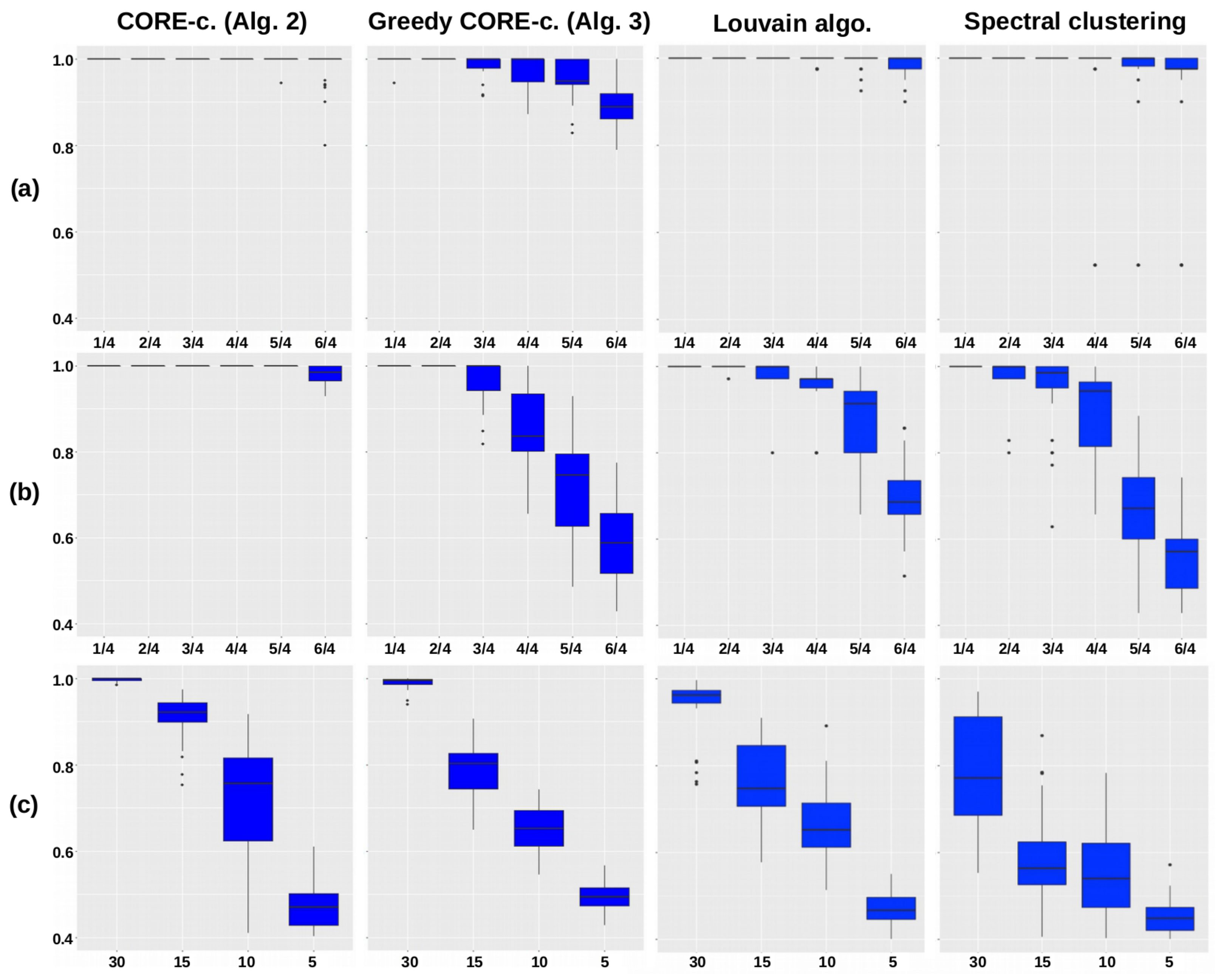
We compared the standard and greedy CORE-clustering algorithms (Algorithms 2 and 3) on these simulated datasets with two other graph-based clustering algorithms: the spectral clustering [30,31], available in the R-package anocva, and Louvain method for community detection [32], available in the R-package igraph. Note that the Louvain method requires as input parameter a graph modeling the dataset (the correlation matrix is transformed upstream into a graph) but not the final number of clusters. Boxplots of the computed scores R (see Equation (5)) are shown in Figure 1. Note that in each boxplot, the dots represent the outlier scores, which are either lower than or higher than , where and are the first and third quartiles of the scores, respectively.
4.2. Application to Real Biological Data
We now present the results obtained on the classic Yeast dataset (https://archive.ics.uci.edu/ml/datasets/Yeast (accessed on 19 February 2021)) [33]. With a total of about weighted edges considered when representing the variables correlations in the graph , the CORE-clustering procedure required about 160 and 3 seconds with Algorithms 2 and 3, respectively.
4.2.1. Yeast Dataset
The well-known synchronized yeast cell cycle data set of [33] includes 77 samples under various time during the cell cycle and a total of 6179 genes, of which 1660 genes are retained for this analysis after pre-processing and filtering. The goal of this analysis is then to detect CORE-clusters among the correlation patterns in the time series of yeast gene expressions measured along the cell cycle. Using this dataset, a measure of similarity between all gene pairs was measured with the absolute value of Pearson’s correlation. A total of about weighted edges are then considered when representing the variables correlations in the graph .
4.2.2. Comparison of the Two CORE-Clustering Algorithms
In order to compare the two proposed CORE-clustering algorithms described (Algorithms 2 and 3) we tested them on the yeast dataset with and . We indeed empirically considered that CORE-clusters containing 30 to 59 variables are reasonable to regularize the problem, and that is a threshold above which the absolute value of the correlation between two variables reasonably shows that their behavior is similar.
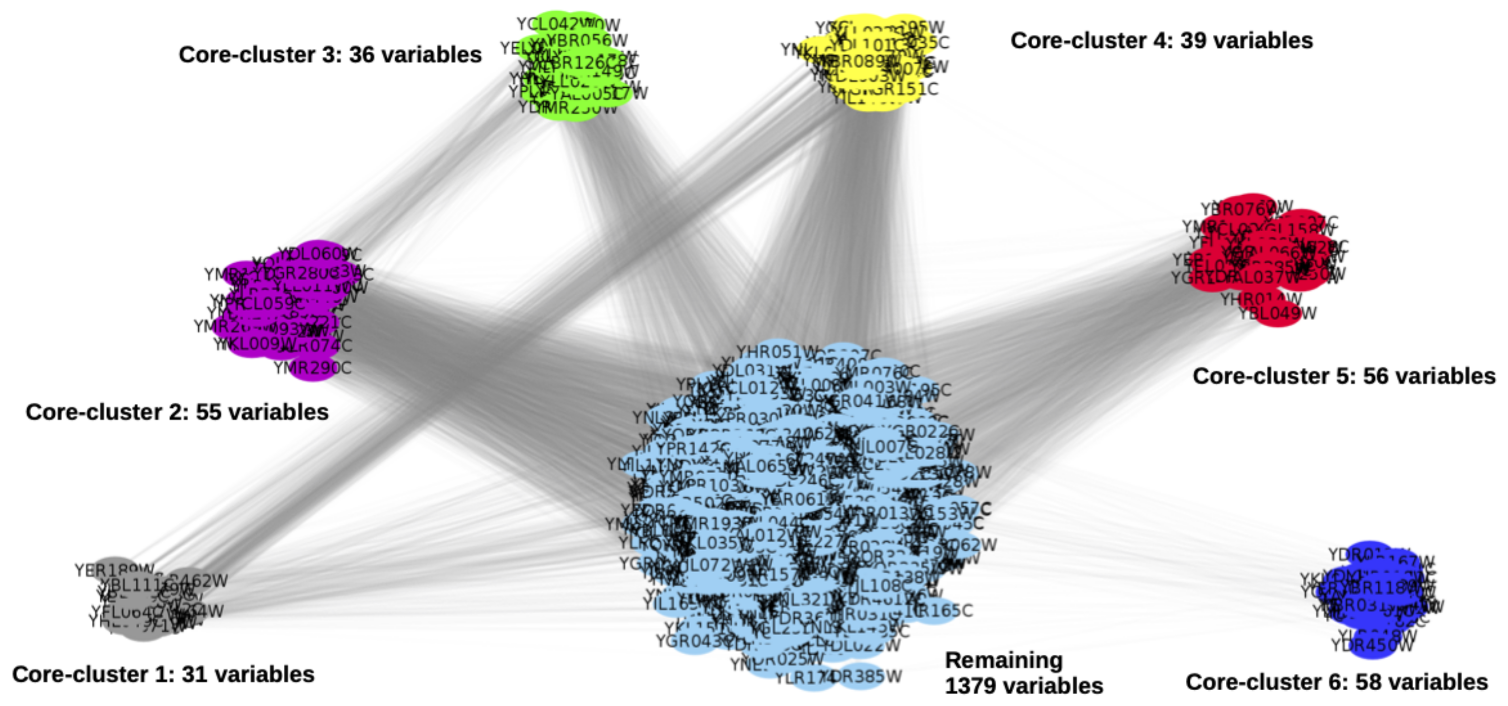
The clustering obtained using the standard algorithm, rows 1 to 19 of Algorithm 2, is shown in Figure 2. In this figure, the represented clusters 1 to 6 have a coherence (see Equation (3)) equals to . Only the clusters 1, 3, 5 and 6 are then considered as CORE-clusters (rows 20 to 25 of Algorithm 2) and their representative variables are RV1 = YER190W, RV3 = YLL026W, RV5 = YDL003W and RV6 = YGL120C. Computational time for the clustering was about 160 s on an Intel(R) Core(TM) i7-6700HQ CPU at 2.60 GHz.
The computations were much faster using the greedy algorithm Algorithm 3. It indeed required about 3 seconds. An amount of 11 CORE-clusters was found. To interpret this result, we computed the coherence c (see Equation (2)) between the 4 representative variables obtained using Algorithm 2 and the 11 obtained using Algorithm 3. Interestingly, Algorithm 3 selected YLL026W = RV3 and YDL003W = RV5. Other variables very close to RV1, RV5 and RV6 (with i.e., higher that the highest within the CORE-clusters) were also selected: YHR219W, YLR103C, YLR276C and YLR196W. Results equal or close to those obtained with Algorithm 2 were then obtained. The representative variables YDR418W, YML119W, YJL038C, YNL283C and YGR167W were additionally found. In this experiment, Algorithm 3 therefore selected more representative variables and has then naturally a larger score (see Equation (4)) than by using Algorithm 2. However, it also obviously captured different representative variables that would be gathered in the same CORE-cluster using Algorithm 2. The two algorithms have therefore slightly different properties but lead to coherent results.
4.2.3. Impact of the Number of Observations
In order to evaluate the stability of the results with respect to the number of observations, we tested again Algorithm 2 with the same parameters, but by using only the 30 first observations of the yeast dataset out of the 77 observations. Interestingly, YDL003W = RV5 was selected and YML093W, which is very close to RV6 (), was also selected. The two other representative variables found, YER190W and YLL026W, were however not similar to RV1 or RV3. The information lost in the 47 observation that we removed therefore did not allowed to recover the influence of RV1 and RV3 on the complex system but the 30 remaining observations contained a sufficient amount of information to detect RV5 and RV6 as influent variables. This suggests that the strategy detects stable representative variables, even when the number of observations is very low compared with the dimension of the observations.
4.2.4. Comparison with Spectral-Clustering
In order to compare our CORE-clustering strategy with a standard clustering approach, we finally estimated representative variables in the Yeast dataset as the center of clusters estimated using spectral clustering. The standard version of the spectral clustering available in R was used. Its main parameter is the number of seeds used in the k-means part of the spectral clustering. When using seeds, an amount of 1 to clusters (with more than one variable) are estimated using k-means and all variables are contained in a cluster. In order to fairly compare the spectral clustering and the CORE-clustering approaches, we then clusterized the variables of the Yeast dataset using . Note that we only tested an higher than 77, due to the fact that observations are known. We tested to evaluate the spectral clustering behaviour with slightly higher than n.
An amount of large clusters were obtained for , respectively. For , only a single cluster gathering almost all variables was also obtained. The average coherence of the estimated clusters was for a standard deviation of . The highest coherence was , which is clearly lower than the considered threshold of that we used with the CORE-clustering. This makes ambiguous the interpretation of the role played by the representative variables.
Finally, it is worth mentioning that all representative variables (genes) obtained using Algorithm 2 have a known physiological function and only two variables out of eleven have an unknown function by using Algorithm 3. For the spectral clustering with , four selected variables out of six have known functions. For , three variables with unknown functions were selected. For , two variables out of three with known functions were selected. For and , the single selected variable was the center of all variables with respect to the center definition in Section 3.3, and turns out to have a known function. It therefore appears in this experiment that the representative variables obtained using CORE-clustering are more interpretable than those estimated using spectral clustering.
4.3. Application to the U.S. Road Network
We now assess the CORE-clustering algorithms on the U.S. road network out of the 9th DIMACS Implementation challenge (http://users.diag.uniroma1.it/challenge9/ (accessed on 19 February 2021)). Our goal here is to discuss the pertinence of the detected CORE-clusters, and not specifically their representative variables, on a large scale and straightforwardly interpretable dataset. The graph contains here nodes, each of them representing a crossing of the U.S. road/streets network, and arcs, representing the part of the roads/streets between two crossings. Interestingly, the distance between the crossings is also associated with each edge of the graph.
To assess the CORE-clustering algorithms on the U.S. road network, we first transformed the distances between the crossings into weights that are higher and higher for increasingly closer crossings. A weight was specifically given to each edge, where l is its original length in feet.
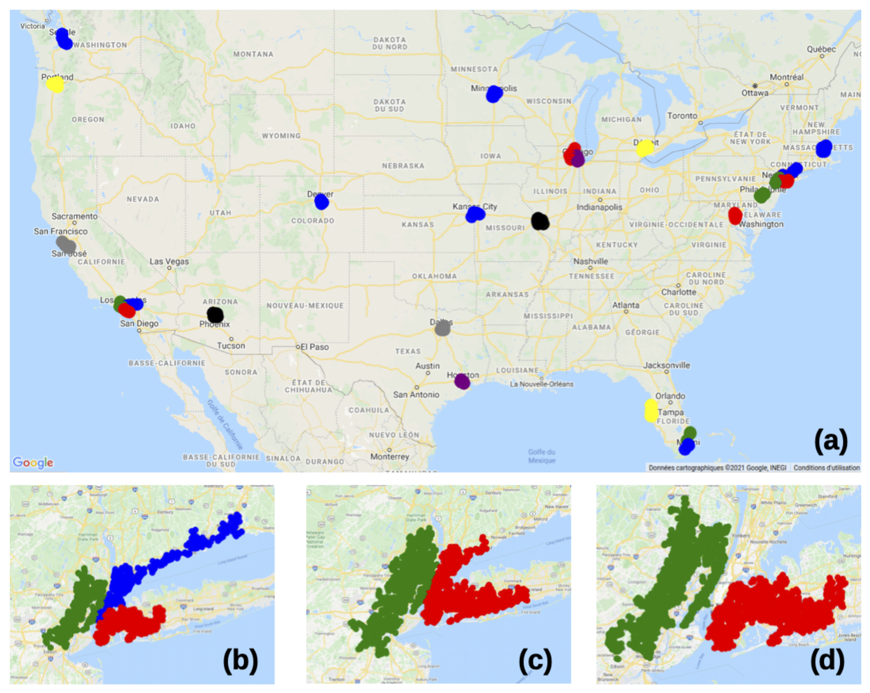
We show Figure 3, the CORE-clusters (Clusters represented using MI Map Tools: GeoPlotter: https://mobisoftinfotech.com/tools/plot-multiple-points-on-map/ (accessed on 19 February 2021)) obtained using the greedy algorithm with and . This means that each CORE-cluster contains a road network of to crossings, for which one can travel from any crossing to another one by only using streets of less than 3996 feet (about km) between two crossings. As expected, the clusters represented in Figure 3 correspond to the 18 largest urban areas in the U.S. Note that two of them are made of three CORE-clusters (New York City and Los Angeles), and two other ones (Miami and Chicago) are made of two CORE-clusters. This is due to an algorithmic choice, discussed in Section 3.2.2 and Section 3.2.3, which leads to the detection of CORE-clusters containing to nodes by using the proposed CORE-clustering algorithms. As discussed in Section 2.6, an interesting strategy if connected CORE-clusters are found consists in running again the CORE-clustering algorithms with higher values of or , to potentially detect more robust CORE-clusters: By reproducing this test with instead of , we now try to find CORE-clusters containing to crossings, only 5 urban areas are found: New York City (2 CORE-clusters), Los Angeles, Chicago, Miami and San Fransisco. Now, by using and now , i.e., with distances between the crossings lower than about 2000 feet (about km) instead of 3996 feet, only 3 urban areas are found: New York City (2 CORE-clusters), Los Angeles and Chicago.
What is interesting here in terms of interpretability is that we have been able to select specific subparts of the U.S. road network by explicitly controling the size of the clusters or a specific level of density in the network. This notion of interpretability can be further discussed by observing the CORE-clusters obtained in the New York city urban area, as shown in Figure 3b–d. By using and , the three CORE-clusters split the densest parts of the New York City urban area into the New Jersey state, Long Island and the rest of New York state. When having larger CORE-clusters, i.e., with , the New Jersey cluster, expands and the densest parts of the two New York state clusters are merged. Now, when enforcing instead a stronger coherence inside of the clusters, i.e., with and , the New Jersey and Long Island CORE-clusters remain stable, but the Manhattan/mainland New York state cluster is not large and dense enough, so it is not captured as a CORE-cluster. Note that each CORE-cluster estimation required about 50 s and 2.4 GB here without any parallelization.
5. Conclusions
Although complex systems in high dimensional spaces with a limited number of observations are quite common across many fields, having efficient methods to treat the associated problem of graph clustering is an ambiguous task. Some of these techniques, based on assumptions in view of controlling the variables contribution to the global clustering, often do not allow to select the best graph partition. In reply to this issue, we developed a formalism based on an original graph clustering strategy with specific properties. This formalism makes it possible to robustly identify groups of representative variables of the studied system by tuning two intuitive parameters: (1) the minimum number of variables in each CORE-cluster, and (2) a minimum level of similarity between all the variables of a CORE-cluster. Its effectiveness was further satisfactorily assessed on simulated data and on real datasets.
From a methodological perspective, an interesting research direction would be to mix Algorithms 2 and 3 into a single hybrid top-down and bottom-up optimization scheme. Our goal would be to scale well to very high dimensional datasets, as when using Algorithm 3, while being as robust as Algorithm 2 when potential CORE-clusters are coarsely identified. When the CORE-clusters found by either Algorithms 2 or 3 are very large, a stochastic strategy could also make faster the detection of their representative variables. Although this secondary part of our methodology has been addressed by using a standard Dijkstra’s algorithm (see Section 3.3), it could be addressed by using an extension of [34] where the optimal paths between all variables would not be pre-computed prior to the central variable detection. Application of our formalism in various fields such as gene regulatory networks, social networks or recommender systems would also be of interest. Our formalism is indeed sufficiently flexible to incorporate different types of similarity measures between the observed variables.
Note finally that our formalism was implemented in C++ and wrapped in a R package, which is freely available on sourceforge (https://es.sourceforge.net/projects/core-clustering/ (accessed on 19 February 2021)), so that these results can be easily reproduced.
Author Contributions
Conceptualization, J.-M.L. and A.-C.B.; methodology, J.-M.L. and L.R.; software, C.C. and L.R.; validation, C.C. and L.R.; formal analysis, L.R.; investigation, J.-M.L. and L.R.; resources, J.-M.L.; data curation, A.-C.B., C.C. and L.R.; writing—original draft preparation, C.C., J.-M.L. and L.R.; writing—review and editing, C.C., J.-M.L. and L.R.; visualization, C.C. and L.R.; supervision, J.-M.L. and L.R.; project administration, J.-M.L. and L.R.; funding acquisition, J.-M.L. and R.B. All authors have read and agreed to the published version of the manuscript.
Funding
Research partially supported by the AI Interdisciplinary Institute ANITI, which is funded by the French “Investing for the Future—PIA3” program under the Grant agreement ANR-19-PI3A-0004.
Institutional Review Board Statement
Not applicable.
Informed Consent Statement
Not applicable.
Data Availability Statement
The data used in this study are openly available at the webpages https://archive.ics.uci.edu/ml/datasets/Yeast (accessed on 19 February 2021) for the Yeast dataset and http://users.diag.uniroma1.it/challenge9/ (accessed on 19 February 2021) for the road network dataset. Examples of synthetic data can be found in the CORE-clustering package https://sourceforge.net/projects/core-clustering/ (accessed on 19 February 2021).
Conflicts of Interest
The authors declare no conflict of interest.
Appendix A. Pertinence of the Representative Variable Detection Model
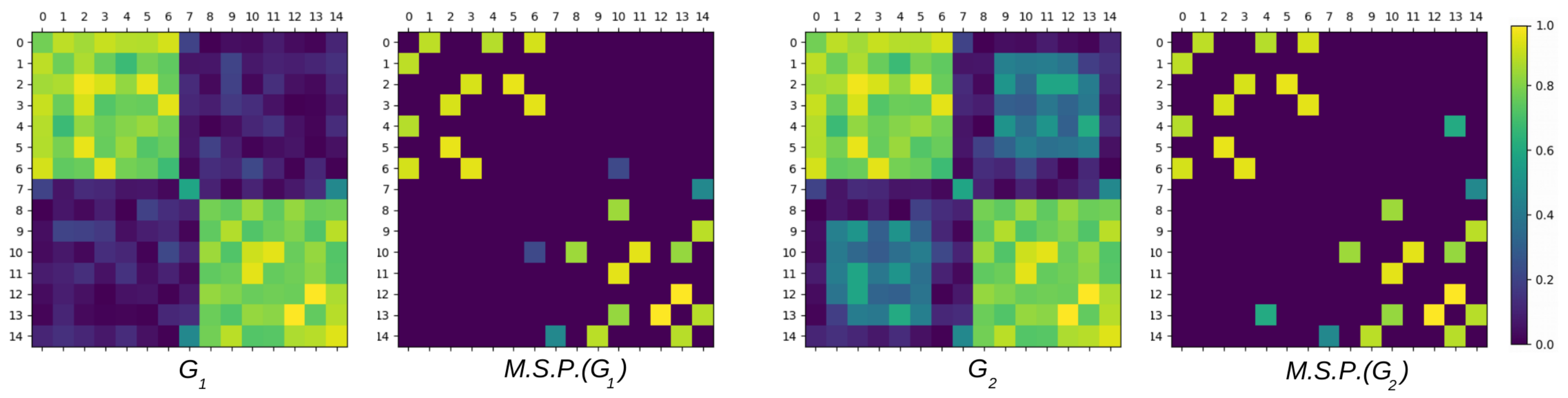
We illustrate, in this section, the notion of coherence defined in Section 2.2. We simulated an adjacency matrix that mimics the absolute values of the Pearson correlations between 15 variables. This symmetric matrix is shown in Figure A1 (top-left) and represents graph following the method of Section 2.1. Each of its values is then equal to a similarity level encoded in between two variables and , where i and j are in . We can clearly remark that it contains two blocks of related variables and and an independent variable . In addition, variables and are slightly more related to other variables in and ,respectively. They can then be considered as the most pertinent representative variables in these blocks. We also added to undesirable relations having an intermediate level between the variables and and saved the result in graph , as shown in Figure A1 (top-right). More quantitatively, the reference blocks and have inner similarities sampled following the normal law ; the background ones are sampled following , and in Figure A1, the undesirable relations are sampled following . In each reference block, the relation between the simulated reference variables and other variables are finally sampled following . The norms of these similarities are then considered and the similarities higher than one are set to one.
We will measure hereafter the coherence of different variable subsamples to illustrate this notion and make clear its interest in the CORE-clustering context. As the CORE-clustering algorithms proposed in Section 3 use maximal spanning trees, we will additionally discuss the corresponding coherences obtained on the maximal spanning trees of and , which are shown in Figure A1 (bottom). The estimated representative variables will finally be given in all tests to make sure that their estimation is robust.
Figure A1.
Adjacency matrices of the simulated graphs and of Appendix A and their maximum spanning trees (ST).
Figure A1.
Adjacency matrices of the simulated graphs and of Appendix A and their maximum spanning trees (ST).

Appendix A.1. Illustration of the Coherence
We give Table A1 the coherence of four pairs of tested CORE-clusters on , and their maximal spanning trees. Corresponding estimated representative variables are given in Table A2. The tested CORE-clusters are: (Test 1) The reference blocks of variables and , i.e., and . (Test 2) Subsamples of and of size three, i.e., and . (Test 3) Samples and in which a variable was replaced with the independent variable , i.e., and . (Test 4) Samples and in which the variables and were swapped, i.e., and .

Table A1.
Coherence of the CORE-clusters tested Appendix A on and . Corresponding representative variables are given Table A2.
Table A1.
Coherence of the CORE-clusters tested Appendix A on and . Corresponding representative variables are given Table A2.
| 0.77 | 0.85 | 0.77 | 0.77 | 0.18 | 0.25 | 0.15 | 0.19 | |
| 0.77 | 0.85 | 0.77 | 0.77 | 0.18 | 0.25 | 0.40 | 0.47 |
Let us first interpret the results in Table A1. The coherences’ first row on in tests and first show that similar coherences were obtained with CORE-clusters of size 7 and 3, although the coherences are slightly higher for smaller CORE-clusters. These coherences are also clearly higher for those obtained in tests and where all variables are not contained in the same simulated block. Interestingly, the results obtained on graph are similar to those obtained on . The only difference here is that the coherences of are slightly higher than in , but still relatively low. Note that the tested CORE-clusters may lead to disconnected subgraphs when tested on the maximum spanning trees. Equation (2) does not make sense in this case. When the simulated subgraphs were connected (12 cases out of 16), we obtained the same coherences on the maximum spanning trees and the whole graph. As discussed in Section 2.4, the coherence of a given CORE-cluster on a maximum spanning tree is indeed lower or equal to the coherence of the same CORE-cluster on the whole graph. We however computed the representative variables in all tested cases, as the centrality measure makes sense even on disconnected subgraphs (see Section 3.3). The results in Table A2 show that the estimated representative variables are always in the reference sets and in the tested configurations. They also correspond to the simulated representative variables, and , in most cases, or are very close to these variables. Note that slightly inaccurate reference variables were detected in , and we can clearly see (Figure A1 (top)) that the influence of its simulated representative variable is less obvious than in set .
Table A2.
Representative variables of the CORE-clusters tested Appendix A on and . Corresponding coherences are given Table A1.
Table A2.
Representative variables of the CORE-clusters tested Appendix A on and . Corresponding coherences are given Table A1.
| 4 | 11 | 3 | 11 | 5 | 11 | 6 | 11 | |
| 4 | 11 | 3 | 11 | 5 | 11 | 3 | 11 |
Appendix A.2. Influence of the Undesirable Relations
We further study the influence of the undesirable relations between and in graph by simulating these relations with different strengths. In the previous subsection, undesirable relations were sampled following , where . Here, we sampled 100 graphs for each strength . For each graph, we then measured the portion of representative variable estimates in the true reference block of variables and the portion of representative variable estimates that are the ground truth representative variables.
Results are given in Table A3 and show that the representative variables detection is particularly stable in these tests, even for large values of . All estimated representative variables are indeed in the true block of variables, except in Test 4 (where two variables of the reference sets are swapped) with , i.e., with the same level of similarity as between the blocks representative variables and the other variables they contain. False estimations are however uncommon even in this case. Exact estimates of the representative variables are naturally less frequent, as this test is more strict. They are however always clearly higher than random estimations which would have portions equal to . The estimates of pertinent representative variables therefore appear as robust, even with strong undesirable relations in the variable similarities and tested CORE-clusters which contain undesirable variables.
Table A3.
Portion of representative variable estimates contained in the proper reference block of variables (main value) and corresponding to the ground truth representative variables (between brackets). Each portion was computed on 100 simulated graphs () and their corresponding maximum spanning trees (). For each group of 100 graphs, a different strength of the undesirable relations is tested.
| Test 1 | Test 2 | Test 3 | Test 4 | |||||
|---|---|---|---|---|---|---|---|---|
| 1. (0.88) | 1. (0.82) | 1. (0.79) | 1. (0.80) | 1. (0.40) | 1. (0.75) | 1. (0.59) | 1. (0.79) | |
| 1. (0.87) | 1. (0.79) | 1. (0.78) | 1. (0.83) | 1. (0.46) | 1. (0.80) | 1. (0.75) | 1. (0.84) | |
| 1. (0.88) | 1. (0.79) | 1. (0.78) | 1. (0.84) | 1. (0.44) | 1. (0.74) | 1. (0.88) | 1. (0.78) | |
| 1. (0.92) | 1. (0.72) | 1. (0.75) | 1. (0.69) | 1. (0.47) | 1. (0.62) | 1. (0.93) | 0.96 (0.71) | |
| 1. (0.92) | 1. (0.59) | 1. (0.70) | 1. (0.48) | 1. (0.49) | 1. (0.44) | 1. (0.93) | 0.89 (0.59) | |
References
- Liu, Z.; Barahona, M. Graph-based data clustering via multiscale community detection. Appl. Netw. Sci. 2020, 5, 3. [Google Scholar] [CrossRef] [Green Version]
- Boccaletti, S.; Latora, V.; Moreno, Y.; Chavez, M.; Hwang, D.U. Complex networks: Structure and dynamics. Phys. Rep. 2006, 424, 175–308. [Google Scholar] [CrossRef]
- Newman, M. Networks: An Introduction; Oxford University Press: Oxford, UK, 2009. [Google Scholar]
- MacQueen, J.B. Proceedings of the Fifth Berkeley Symposium on Mathematical Statistics and Probability; University of California Press: Berkeley, CA, USA, 1967; Volume 1, pp. 281–297. [Google Scholar]
- Seidman, S.B. Network structure and minimum degree. Soc. Netw. 1983, 5, 269–287. [Google Scholar] [CrossRef]
- Giatsidis, C.; Malliaros, F.D.; Thilikos, D.M.; Vazirgiannis, M. CORECLUSTER: A degeneracy based graph clustering framework. In Proceeding of the Twenty-Eight AAAI Conference on Artificial Intelligence, Québec City, QC, Canada, 27–31 July 2014. [Google Scholar]
- Batagelj, V.; Zaversnik, M. Fast algorithms for determining (generalized) core groups in social networks. Adv. Data Anal. Classif. 2011, 5, 129–145. [Google Scholar] [CrossRef]
- Agarwal, P.K.; Har-Peled, S.; Varadarajan, K.R. Geometric approximation via coresets. In Combinatorial and Computational Geometry; MSRI University Press: Berkeley, CA, USA, 2005; pp. 1–30. [Google Scholar]
- Claici, S.; Genevay, A.; Solomon, J. Wasserstein Measure Coresets. arXiv 2020, arXiv:1805.07412. [Google Scholar]
- Baharan, M.; Kaidi, C.; Jure, L. Coresets for robust training of deep neural networks against noisy labels. In In Proceedings of the Neural Information Processing Systems (NeurIPS 2020), Vancouver, BC, Canada, 6–12 December 2020. [Google Scholar]
- Baykal, C.; Liebenwein, L.; Gilitschenski, I.; Feldman, D.; Rus, D. Data-dependent coresets for compressing neural networks with applications to generalization bounds. arXiv 2018, arXiv:1804.05345. [Google Scholar]
- Bachem, O.; Lucic, M.; Lattanzi, S. One-shot coresets:The case of k-clustering. In Proceeding of the International Conference on Artificial Intelligence and Statistics (AISTATS), Playa Blanca, Spain, 9–11 April 2018; pp. 784–792. [Google Scholar]
- Saeys, Y.; Inza, I.; Larranaga, P. A review of feature selection techniques in bioinformatics. Bioinformatics 2007, 23, 2507–2517. [Google Scholar] [CrossRef] [PubMed] [Green Version]
- Zhao, Z.; Morstatter, F.; Sharma, S.; Alelyani, S.; Anand, A.; Liu, H. Advancing Feature Selection Research. in ASU Feature Selection Repository. 2010, pp. 1–28. Available online: http://www.public.asu.edu/huanliu/papers/tr-10-007.pdf (accessed on 14 January 2021).
- Li, J.; Cheng, K.; Wang, S.; Morstatter, F.; Trevino, R.P.; Tang, J.; Liu, H. Feature Selection: A Data Perspective. ACM Comput. Surv. 2018, 50, 94:1–94:45. [Google Scholar] [CrossRef] [Green Version]
- Wu, C.; Ioannidis, S.; Szaier, M.; Li, X.; Kaeli, D.; Dy, J. Iterative Spectral Method for Alternative Clustering. Proc. Mach. Learn. Res. 2018, 84, 115–123. [Google Scholar]
- Chen, J.; Chang, Y.; Castaldi, P.; Cho, M.; Hobbs, B.; Dy, J. Crowdclustering with Partitions Labels. Proc. Mach. Learn. Res. 2018, 84, 1127–1136. [Google Scholar]
- Yu, L.; Liu, H. Feature Selection for High-Dimensional Data: A Fast Correlation-Based Filter Solution. In Proceedings of the International Conference on Machine Learning (ICML-2003), Washington, DC, USA, 21–24 August 2003; pp. 856–863. [Google Scholar]
- Brunet, A.C.; Loubes, J.M.; Azais, J.M.; Courtney, M. Method of Identification of a Relationship between Biological Elements. WO Patent App. PCT/EP2015/060,779, 3 December 2015. [Google Scholar]
- Brunet, A.C.; Azais, J.M.; Loubes, J.M.; Amar, J.; Burcelin, R. A new gene co-expression network analysis based on Core Structure Detection (CSD). arXiv 2016, arXiv:1607.01516. [Google Scholar]
- Pollack, M. The Maximum Capacity through a Network. Oper. Res. 1960, 8, 733–736. [Google Scholar] [CrossRef]
- Hu, T.C. The Maximum Capacity Route Problem. Oper. Res. 1961, 9, 898–900. [Google Scholar] [CrossRef] [Green Version]
- Randall, K.H. Cilk: Efficient Multithreaded Computing. Ph.D. Thesis, Massachusetts Institute of Technology, Cambridge, MA, USA, 1998. [Google Scholar]
- Cysouw, M. R Function Cor.Sparse. 2018. Available online: https://www.rdocumentation.org/packages/qlcMatrix/versions/0.9.2/topics/cor.sparse (accessed on 2 February 2018).
- Kruskal, J.B. On the Shortest Spanning Subtree of a Graph and the Traveling Salesman Problem. Proc. Am. Math. Soc. 1956, 7, 48–50. [Google Scholar] [CrossRef]
- Tarjan, R. Depth first search and linear graph algorithms. SIAM J. Comput. 1972, 1, 146–160. [Google Scholar] [CrossRef]
- Steele, J.M. Minimal spanning trees for graphs with random edge lengths. In Mathematics and Computer Science II; Springer: Berlin/Heidelberg, Germany, 2002; pp. 223–245. [Google Scholar]
- Cormen, T.H.; Leiserson, C.E.; Rivest, R.L.; Stein, C. Introduction to Algorithms; MIT Press: Cambridge, MA, USA, 2001. [Google Scholar]
- Zan, B.F.; Noon, C.E. Shortest Path Algorithms: An Evaluation Using Real Road Networks. Transp. Sci. 1998, 32, 65–73. [Google Scholar] [CrossRef]
- Shi, J.; Malik, J. Normalized cuts and image segmentation. IEEE Trans. Pattern Anal. Mach. Intell. 2000, 22, 888–905. [Google Scholar]
- Ng, A.; Jordan, M.; Weiss, Y. On spectral clustering: Analysis and an algorithm. In Proceedings of the Advances in Neural Information Processing Systems (NIPS 2002), Vancouver, BC, Canada, 9–14 December 2002; pp. 849–856. [Google Scholar]
- Blondel, V.; Guillaume, J.; Lambiotte, R.; Lefebvre, E. Fast unfolding of communities in large networks. J. Stat. Mech. Theory Exp. 2008, 10008. [Google Scholar] [CrossRef] [Green Version]
- Spellman, P.T.; Sherlock, G.; Zhang, M.Q.; Vishwanath, I.R.; Anders, K.; Eisen, M.B.; Brown, P.O.; Botstein, D.; Futcher, B. Comprehensive Identification of Cell-Cycle-regulated Genes of Yeast Saccharomyces cerevisiae by Microarray Hybridization. Mol. Biol. Cell 1998, 9, 3273–3297. [Google Scholar] [CrossRef] [PubMed]
- Gadat, S.; Gavra, I.; Risser, L. How to calculate the barycenter of a weighted graph. Informs 2018, 43. [Google Scholar] [CrossRef] [Green Version]
Figure 1.
Boxplots of the scores R (see Section 4.1.2) obtained on simulated datasets using the standard and the greedy CORE-clustering algorithms as well as the Louvain and the Spectral clustering algorithms. A score of 1 reflects a purely accurate detection of the simulated clusters and the lower this score, the lower the accuracy. The boxplots were obtained by reproducing 30 times the procedure of Section 4.1.1. (a) Two simulated clusters with noise levels ranging from to . (b) Same as (a) with five simulated clusters. (c) Five clusters simulated using 30, 15, 10 and 5 observations and a noise level of .

Figure 2.
CORE-clusters obtained using Algorithm 2 on the yeast dataset of [33] and the granularity coefficient . CORE-clusters containing 30 to 59 variables are then estimated.
Figure 2.
CORE-clusters obtained using Algorithm 2 on the yeast dataset of [33] and the granularity coefficient . CORE-clusters containing 30 to 59 variables are then estimated.

Figure 3.
Results obtained using the greedy CORE-clustering algorithm on the U.S. road network (≈ nodes) in about one minute. (a,b) CORE-clusters obtained using and represented in the U.S. and in New York City urban area. (c) CORE-clusters obtained using and represented in New York City urban area only. (d) CORE-clusters obtained using and represented in New York City urban area only. Background: Google maps. Clusters represented using MI Map Tools: GeoPlotter.

Publisher’s Note: MDPI stays neutral with regard to jurisdictional claims in published maps and institutional affiliations. |
© 2021 by the authors. Licensee MDPI, Basel, Switzerland. This article is an open access article distributed under the terms and conditions of the Creative Commons Attribution (CC BY) license (http://creativecommons.org/licenses/by/4.0/).
Share and Cite
MDPI and ACS Style
Champion, C.; Brunet, A.-C.; Burcelin, R.; Loubes, J.-M.; Risser, L. Detection of Representative Variables in Complex Systems with Interpretable Rules Using Core-Clusters. Algorithms 2021, 14, 66. https://doi.org/10.3390/a14020066
AMA Style
Champion C, Brunet A-C, Burcelin R, Loubes J-M, Risser L. Detection of Representative Variables in Complex Systems with Interpretable Rules Using Core-Clusters. Algorithms. 2021; 14(2):66. https://doi.org/10.3390/a14020066
Chicago/Turabian StyleChampion, Camille, Anne-Claire Brunet, Rémy Burcelin, Jean-Michel Loubes, and Laurent Risser. 2021. "Detection of Representative Variables in Complex Systems with Interpretable Rules Using Core-Clusters" Algorithms 14, no. 2: 66. https://doi.org/10.3390/a14020066
Note that from the first issue of 2016, this journal uses article numbers instead of page numbers. See further details here.