Some Notes on the Omega Distribution and the Pliant Probability Distribution Family

Abstract

In 2020 Dombi and Jónás (Acta Polytechnica Hungarica 17:1, 2020) introduced a new four parameter probability distribution which they named the pliant probability distribution family. One of the special members of this family is the so-called omega probability distribution. This paper deals with one of the important characteristic “saturation” of these new cumulative functions to the horizontal asymptote with respect to Hausdorff metric. We obtain upper and lower estimates for the value of the Hausdorff distance. A simple dynamic software module using CAS Mathematica and Wolfram Cloud Open Access is developed. Numerical examples are given to illustrate the applicability of obtained results.

1. Introduction

This paper deals with the asymptotic behavior of the Hausdorff distance between Heaviside function and some novel distribution functions. The study can be very useful for specialists that are working in several scientific fields like insurance, financial mathematics, analysis, approximation of data sets in various modeling problems and others. Application of the Hausdorff metrics in different approximation problems is topic for many science works (for example see articles [1,2,3,4,5,6,7,8], some monographs [9,10,11,12,13,14,15,16,17,18] and references there in).

Definition 1.

The shifted Heaviside step function is defined by

$$h_{t_0}\left(t\right)=\left\{\begin{array}{cc}0\hfill & \mathit{if}t<t_0,\hfill \\ \left[0,1\right]\hfill & \mathit{if}t=t_0,\hfill \\ 1\hfill & \mathit{if}t>t_0.\hfill \end{array}\right.$$

The theory of Hausdorff approximations is due to Bulgarian mathematician Blagovest Sendov. His work and achievements are connected to the approximation of functions with respect to Hausdorff distance.

Definition 2.

[19] The Hausdorff distance (the H-distance) $\rho (f,g)$ between two interval functions $f,g$ on $\Omega \subseteq \mathbb{R}$, is the distance between their completed graphs $F\left(f\right)$ and $F\left(g\right)$ considered as closed subsets of $\Omega \times \mathbb{R}$. More precisely,

$$\rho (f,g)=max\{\underset{A\in F\left(f\right)}{sup}\underset{B\in F\left(g\right)}{inf}\parallel A-B\parallel ,\underset{B\in F\left(g\right)}{sup}\underset{A\in F\left(f\right)}{inf}\parallel A-B\parallel \},$$

wherein $\parallel \dot{\parallel }$ is any norm in ${\mathbb{R}}^2$, e.g., the maximum norm $\parallel (t,x)\parallel =max\left\{\right|t|,|x\left|\right\}$; hence the distance between points $A=(t_A,x_A)$, $B=(t_B,x_B)$ in ${\mathbb{R}}^2$ is $\parallel A-B\parallel =max\left(\right|t_A-t_B|,|x_A-x_B\left|\right)$.

In 2019 Dombi et al. [20] (see also [21]) suggested an auxiliary function that is called the omega function.

Definition 3.

The omega function ${\omega }_m^{(\alpha ,\beta )}\left(x\right)$ is given by

$${\omega }_m^{(\alpha ,\beta )}\left(x\right)={\left(\frac{m^{\beta }+x^{\beta }}{m^{\beta }-x^{\beta }}\right)}^{\frac{\alpha m^{\beta }}{2}},$$

(1)

where $\alpha ,m\in \mathbb{R}$, $m>0$, $\beta \in {\mathit{B}}_{\gamma }$, $x\in \left({\displaystyle \frac{m}{2}(\gamma -1),m}\right)$, $\gamma \in \{-1,1\}$ with the domain set ${\mathit{B}}_{\gamma }=\{b^{-\frac{1}{2}(\gamma +1)}:b\in {\mathbb{R}}^{+},\gamma \in \{-1,1\}\}$.

The authors presented some main properties of the omega function as domain, differentiability, monotonicity, limits and convexity. One of the important properties is that the omega function ${\omega }_m^{(\alpha ,\beta )}$ ($\alpha ,\beta ,m\in \mathbb{R}$, $\beta ,m>0$) and the exponential function $f\left(x\right)=e^{\alpha x^{\beta }}$ ($\alpha ,\beta \in \mathbb{R}$, $\beta >0$) may be derived from a common differential equation. Once more it is shown that omega function is asymptotically identical with the exponential function (for more details see ([20] Theorem 1) and ([21] Proposition 1)). Some probability distributions are founded on this auxiliary function as the omega probability distribution (see [20]) and the pliant probability distribution family (see [21,22]). Hence, some probability distributions, which formulas include exponential terms, also can be approximated using this function, for example, the well-known Weibull, Exponential and Logistic probability distributions.

In this paper, we study the asymptotic behavior of the Hausdorff distance between Heaviside function and the pliant probability distribution function. We study the omega distribution function. We develop a self-intelligent dynamic software module using the obtained results. Several numerical examples are presented.

2. The Pliant Probability Distribution Family

In 2020 based on omega function Dombi and Jónás [21] proposed new four-parameter probability distribution function called the pliant probability distribution function (see also ([22] Chapter 3)).

Definition 4.

The pliant probability distribution function $F_p(x;\alpha ,\beta ,\gamma ,m)$ (pliant CDF) is defined by

$$F_p(x;\alpha ,\beta ,\gamma ,m)=\left\{\begin{array}{cc}0\hfill & \mathit{if}x\le \frac{m}{2}(\gamma -1),\hfill \\ {(1-\gamma {\omega }_m^{(-\alpha ,\beta )}\left(x\right))}^{\gamma }\hfill & \mathit{if}x\in (\frac{m}{2}(\gamma -1),m),\hfill \\ 1\hfill & \mathit{if}x\ge m,\hfill \end{array}\right.$$

(2)

where ${\omega }_m^{(-\alpha ,\beta )}$ is defined by (1) and $\alpha ,m\in \mathbb{R}$, $\alpha >0$, $m>0$, $\beta \in {\mathbf{B}}_{\gamma }$, $\gamma \in \{-1,1\}$.

According to its properties, this new probability distribution can be applied in many fields of science and in a wide range of modeling problems. The pliant probability distribution is a generalization of the epsilon probability distribution (see [23]). In 2020 Árva noted that the omega probability distribution (see [20]) can be derived from the pliant probability distribution function after reparametrization or by utilizing its asymptotic properties (see ([24] Lemma 2)).

In 2020 Kyurkchiev [25] considered the asymptotic behavior of Hausdorff distance between the shifted Heaviside function and the so-called epsilon probability distribution. Once more he proved a precise bound for the values of Hausdorff distance. He noted that once may formulate the corresponding approximation problem for the omega probability distribution. This is the main purpose of Section 3 of this work.

This section is dedicated to the behavior of the CDF function of the pliant probability distribution and more precisely “saturation to the horizontal asymptote $a=1$ in the Hausdorff sense”.

Let $\alpha ,\beta ,m>0$, $\gamma \in \{-1,1\}$ and $t\in (\frac{m}{2}(\gamma -1),m)$. For the function $F_p(x;\alpha ,\beta ,\gamma ,m)$ given in (2) we have

$$F_p(t_0;\alpha ,\beta ,\gamma ,m)=\frac{1}{2}\mathrm{with}{t}_0=m{\left(\frac{1-z}{1+z}\right)}^{{\beta }^{-1}},z={\left(\frac{1}{\gamma }-\frac{2^{-1/\gamma }}{\gamma }\right)}^{2{\left(\alpha m^{\beta }\right)}^{-1}}.$$

(3)

Then the Hausdorff distance d between $F_p(x;\alpha ,\beta ,\gamma ,m)$ and the Heaviside function $h_{t_0}\left(t\right)$ satisfies the following nonlinear equation

$$F_p(t_0+d;\alpha ,\beta ,\gamma ,m)=1-d.$$

In the next theorem, we prove upper and lower estimates for the Hausdorff approximation d.

Theorem 1.

Let

$$A_p=1+\frac{1}{4}\alpha \beta \gamma m^{\beta -1}(1-2^{-1/\gamma })2^{-\frac{\gamma -1}{\gamma }}\left(\frac{1-z^2}{z}\right){\left(\frac{1-z}{1+z}\right)}^{{\beta }^{-1}}$$

(4)

and $2.1A_p>e^{1.05}$ with z defined by (3). Then for the Hausdorff distance d between shifted Heaviside function $h_{t_0}\left(t\right)$ and the Pliant CDF function $F_p(t;\alpha ,\beta ,\gamma ,m)$ defined by (2) the following inequalities hold true:

$$d_l=\frac{1}{2.1A_p}<d<\frac{ln\left(2.1A_p\right)}{2.1A_p}=d_r.$$

Proof. 

Let us consider the function

$$H\left(d\right)=F_p(t_0+d;\alpha ,\beta ,\gamma ,m)-1+d,$$

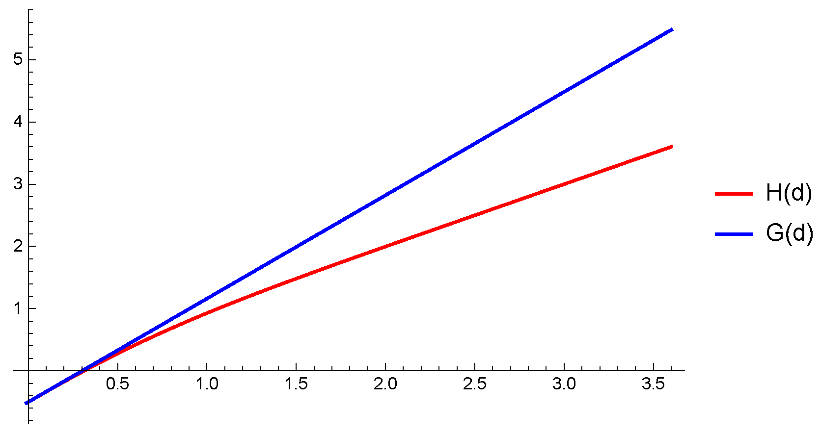
where the pliant CDF function $F_p(t;\alpha ,\beta ,\gamma ,m)$ is defined by (2). It is easy to show that $H^{\prime }\left(d\right)>0$, so the function $H\left(d\right)$ is increasing. We examine the following approximation of $H\left(d\right)$ as we use the function

$$G\left(d\right)=-\frac{1}{2}+A_{p}d,$$

where $A_p$ is given by (4). Indeed from Taylor expansion, we get $G\left(d\right)-H\left(d\right)=\mathcal{O}\left(d^2\right)$. This means that $G\left(d\right)$ approximates $H\left(d\right)$ with $d\to 0$ as $\mathcal{O}\left(d^2\right)$ (see Figure 1). More over $G^{\prime }\left(d\right)>0$ and function $G\left(d\right)$ is also increasing. Let the following condition $2.1A_p>e^{1.05}$ holds. Then it is easy to show that

$$G\left(d_l\right)=-\frac{1}{2}+A_p\frac{1}{2.1A_p}<0\mathrm{and}G\left(d_r\right)=-\frac{1}{2}+A_p\frac{ln\left(2.1A_p\right)}{2.1A_p}>-\frac{1}{2}+\frac{1.05}{2.1}=0.$$

This completes the proof.  □

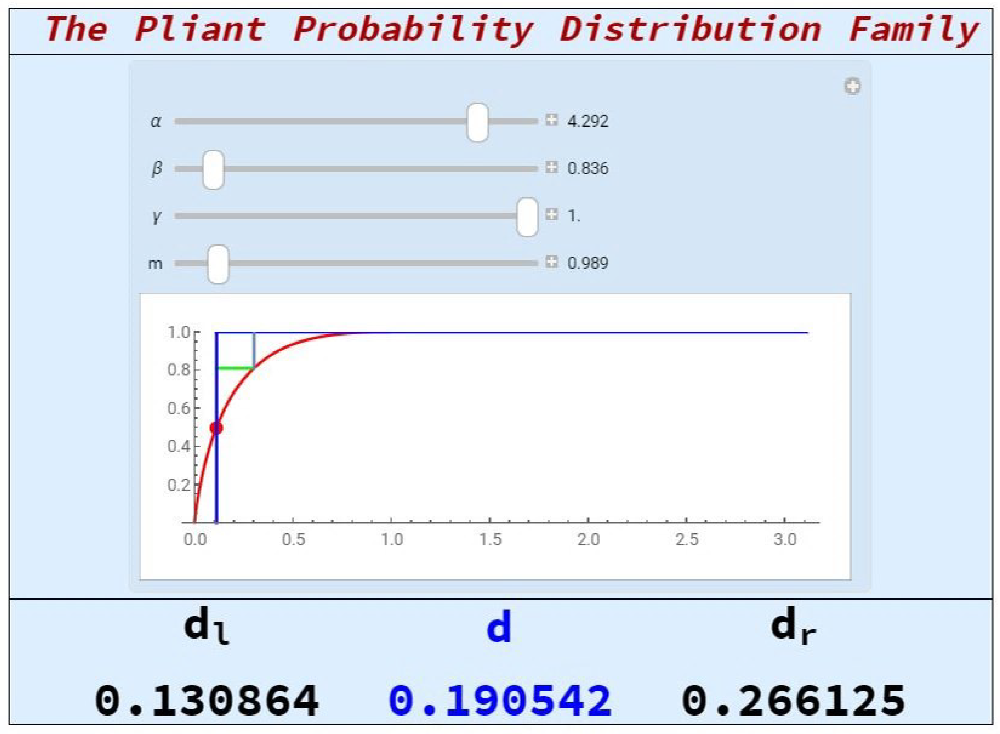
A simple dynamic programming module implemented within the programming environment CAS Wolfram Mathematica and Wolfram Cloud Open Access is developed (see Figure 2). Some of the possibilities of the proposed module are:

• computation of the Hausdorff distance between the Heaviside step function and the Pliant probability distribution function under dynamical user-defined values for parameters $\alpha$, $\beta$, $\gamma$, m;
• automatic check of the conditions from Theorem 1 and computation upper and lower estimates that can be used as confidence bounds;
• tools for dynamical visualization of obtained results;
• web (cloud) version of the module that requires only a browser and internet connection.

Let us consider an example with real data. In [26] Proschan gives the numbers of operating hours between successive failure times of air conditioning systems in Boeing airplanes:

$$\begin{array}{c}1,1,2,3,3,3,3,4,5,5,5,5,5,7,7,7,9,9,10,11,11,11,11,12,12,12,12,13,14,14,14,14,14,14,14,14,\hfill \\ 15,15,15,16,16,16,18,18,18,18,18,18,20,20,21,21,22,22,22,23,23,23,24,24,25,26,26,27,27,29,\hfill \\ 29,29,29,30,31,31,32,33,33,34,34,34,35,35,36,36,37,39,39,41,42,43,44,44,44,46,46,47,47,48,\hfill \\ & & 49,50,50,51,52,54,54,55,56,56,57,57,57,58,59,59,59,60,61,61,62,62,62,63,65,66,67,67,68,70,\hfill \\ 70,71,71,72,74,76,77,79,79,80,82,84,85,87,88,90,90,91,95,97,97,98,100,100,101,102,102,104,\hfill \\ 104,104,106,111,118,118,120,120,130,130,130,134,139,141,142,152,153,156,163,169,176,181,\hfill \\ 182,184,186,188,191,194,197,201,206,208,208,209,210,216,220,225,230,230,239,246,246,254,\hfill \\ 261,270,283,310,320,326,359,386,413,438,447,487,493,502,603.\hfill \end{array}$$

In [27] Okorie and Nadarajah analyzed this data set. Applying the method of maximum likelihood, they received that this data set can be approximated with the pliant probability distribution with parameters $\alpha =4.292$, $\beta =0.836$, $\gamma =1$ and $m=0.989$. In Figure 2 we present the results that we obtain with our programming module for approximation the Heaviside step function and the pliant probability distribution function $F_p(t;\alpha ,\beta ,\gamma ,m)$ with corresponding parameters. Namely, we obtain the values of Hausdorff distance $d=0.190542$, its upper and lower estimates $d_l=0.130864$ and $d_r=0.266125$, respectively. We also get the graphical visualization of the results. It is easy to see that the presented software module can be used from specialists when they make a choice for a model for approximation of cumulative data in various modeling problems. Moreover, upper and lower estimations from Theorem 1 can be used as “confidence bounds”.

In Dombi and Jónás [21] showed in detail that the Pliant probability distribution can approximate well several other functions (see also ([22] Chapter 3)). In

Table 1. Some approximations by the Pliant CDF.

Distribution	Parameters and Domain of the Pliant Probability	Approximated CDF
Weibull	$\alpha >0$, $\beta >0$, $\gamma =1$, $m>0$, $x\in (0,m)$	$F_W(x;\alpha ,\beta )=\left\{\begin{array}{cc}0\hfill & \mathrm{if}x\le 0\hfill \\ {\displaystyle 1-e^{-\alpha x^{\beta }}}\hfill & \mathrm{if}x\ge 0\hfill \end{array}\right.$
Exponential	$\alpha >0$, $\beta =1$, $\gamma =1$, $m>0$, $x\in (0,m)$	$F_{exp}(x;\alpha )=\left\{\begin{array}{cc}0\hfill & \mathrm{if}x\le 0\hfill \\ {\displaystyle 1-e^{-\alpha x}}\hfill & \mathrm{if}x\ge 0\hfill \end{array}\right.$
Logistic	$\alpha >0$, $\beta =1$, $\gamma =-1$, $m>0$, $x\in (-m,m)$	${\displaystyle F_L(x;\alpha )=\frac{1}{{\displaystyle 1+e^{-\alpha x}}}}$
Standard Normal	$\alpha =2\sqrt{2/\pi }$, $\beta =1$, $\gamma =-1$, $m>0$, $x\in (-m,m)$	${\displaystyle \Phi \left(x\right)=\frac{1}{\sqrt{2\pi }}{\int }_{-\infty }^x{e}^{(-t^2/2)}dt}$

are presented some of the special cases.

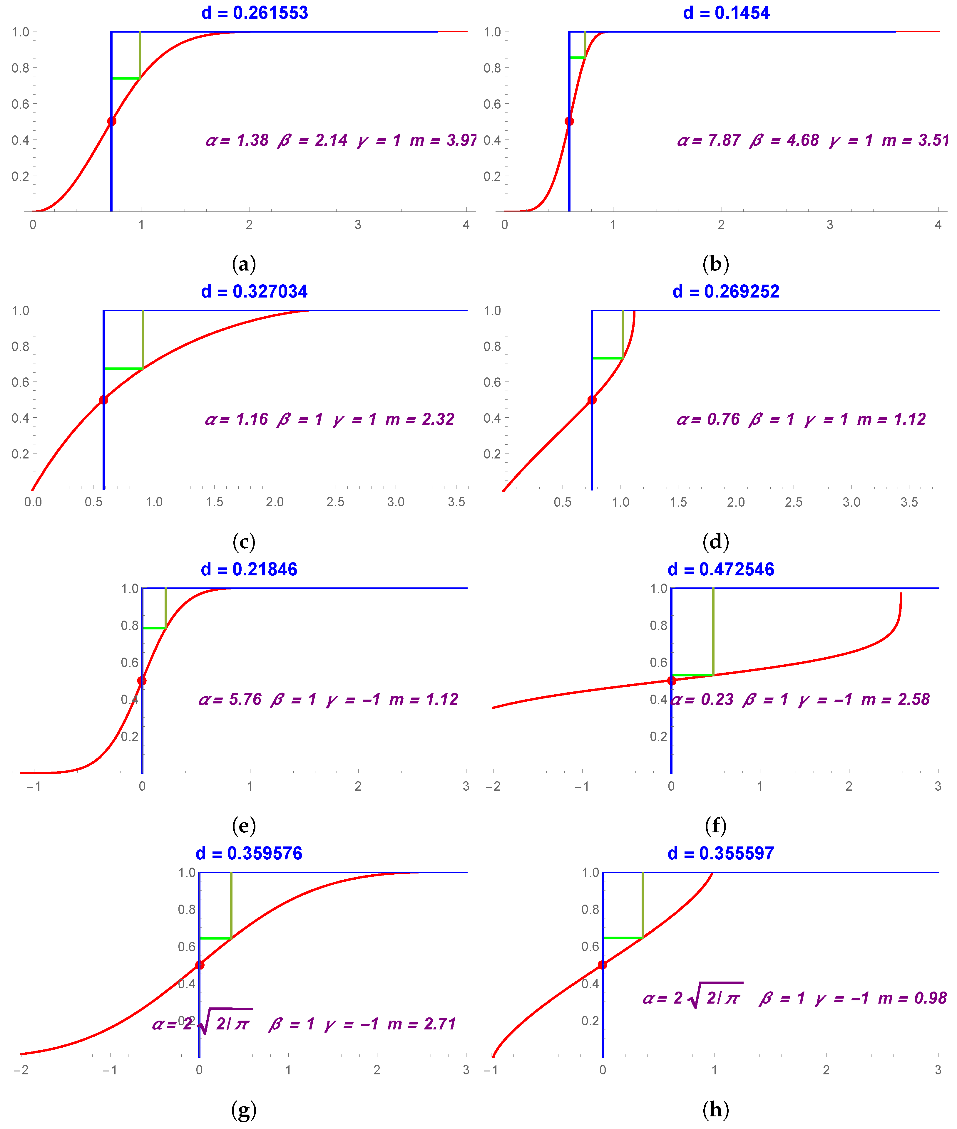
Let us consider some computational examples. The obtained results are presented in

Table 2. Some examples for Pliant probability function $F_p(x;\alpha ,\beta ,\gamma ,m)$.

$\mathit{\alpha }$	$\mathit{\beta }$	$\mathit{\gamma }$	m	d	Figure 3	Approximation Distribution
$1.13$	$2.14$	1	$3.97$	$0.261553$	(a)	Weibull
$7.87$	$4.68$	1	$3.51$	$0.145400$	(b)	Weibull
$1.16$	1	1	$2.32$	$0.327034$	(c)	Exponential
$0.76$	1	1	$1.12$	$0.269252$	(d)	Exponential
$5.76$	1	$-1$	$1.12$	$0.218460$	(e)	Logistic
$0.23$	1	$-1$	$2.58$	$0.472546$	(f)	Logistic
$2\sqrt{2/\pi }$	1	$-1$	$2.71$	$0.359576$	(g)	Standard Normal
$2\sqrt{2/\pi }$	1	$-1$	$0.98$	$0.355597$	(h)	Standard Normal

. In these examples for different values of parameters $\alpha$, $\beta$, $\gamma$, m we calculate the Hausdorff distance between the Heaviside step function $h_{t_0}\left(t\right)$ and the Pliant probability distribution $F_p(x;\alpha ,\beta ,\gamma ,m)$. Graphical results are presented in Figure 3 and it can be seen that the “saturation” is faster. In the last column of Table 2 we show which classical probability distribution can be considered as a approximation of the Pliant probability distribution function.

3. Omega Probability Distribution

Using the omega function Dombi et al. [20] defined the so-called Omega probability distribution. In the next definition, we give the corresponding CDF function.

Definition 5.

The Omega probability cumulative distribution function $F(x;\alpha ,\beta ,m)$ (omega CDF) is defined by

$$F(x;\alpha ,\beta ,m)=\left\{\begin{array}{cc}0\hfill & \mathit{if}x\le 0,\hfill \\ 1-{\omega }_m^{(-\alpha ,\beta )}\left(x\right)\hfill & \mathit{if}0<x<m,\hfill \\ 1\hfill & \mathit{if}x\ge m,\hfill \end{array}\right.$$

(5)

where ${\omega }_m^{(-\alpha ,\beta )}$ is defined by (1) and $\alpha ,\beta ,m\in \mathbb{R}$, $\beta ,m>0$, $x\in (0,m)$.

In this section, we investigate the omega probability distribution in Hausdorff sense as a continuation of the work of Kyurkchiev [25] and as a corollary of the pliant probability distribution.

Let $\alpha ,\beta ,m>0$ and $t\in (0,m)$. For the function $F(x;\alpha ,\beta ,m)$ given in (5) we have

$$F(t_0;\alpha ,\beta ,m)=\frac{1}{2}\mathrm{with}{t}_0=m{\left(\frac{2^{2{\left(\alpha m^{\beta }\right)}^{-1}}-1}{2^{2{\left(\alpha m^{\beta }\right)}^{-1}}+1}\right)}^{{\beta }^{-1}}.$$

Then the Hausdorff distance d between $F(t;\alpha ,\beta ,m)$ and the Heaviside function $h_{t_0}\left(t\right)$ satisfies the following nonlinear equation

$$F(t_0+d;\alpha ,\beta ,m)=1-d$$

or

$${\left(\frac{m^{\beta }+{(t_0+d)}^{\beta }}{m^{\beta }-{(t_0+d)}^{\beta }}\right)}^{\frac{\alpha m^{\beta }}{2}}=\frac{1}{d}.$$

The next theorem is a corollary of Theorem 1 in the case of the omega distribution.

Theorem 2.

Let

$$A=1+\frac{1}{8}\alpha \beta m^{\beta -1}\left(\frac{4^{2{\left(\alpha m^{\beta }\right)}^{-1}}-1}{4^{{\left(\alpha m^{\beta }\right)}^{-1}}}\right){\left(\frac{4^{{\left(\alpha m^{\beta }\right)}^{-1}}+1}{4^{{\left(\alpha m^{\beta }\right)}^{-1}}-1}\right)}^{{\beta }^{-1}}$$

and $2.1A>e^{1.05}$. Then for the Hausdorff distance d between shifted Heaviside function $h_{t_0}\left(t\right)$ and the Omega CDF function $F(t;\alpha ,\beta ,m)$ defined by (5) the following inequalities hold true:

$$d_l=\frac{1}{2.1A}<d<\frac{ln\left(2.1A\right)}{2.1A}=d_r.$$

(6)

In

Table 3. Some bounds for Hausdorff distance d by (6).

$\mathit{\alpha }$	$\mathit{\beta }$	m	${\mathit{d}}_{\mathit{l}}$	d	${\mathit{d}}_{\mathit{r}}$	Figure 4
$0.87$	$0.98$	$4.51$	$0.330061$	$0.361465$	$0.365865$	(a)
$0.86$	$0.97$	$6.56$	$0.333677$	$0.365581$	$0.366238$	(b)
$0.33$	$1.88$	$3.85$	$0.328542$	$0.350978$	$0.365697$	(c)
$0.54$	$3.11$	$7.84$	$0.238728$	$0.259147$	$0.341961$	(d)
$3.01$	$0.39$	$2.13$	$0.067058$	$0.180506$	$0.181204$	(e)
$2.35$	$0.53$	$8.76$	$0.166522$	$0.254183$	$0.298512$	(f)
$2.64$	$3.21$	$4.81$	$0.177190$	$0.198820$	$0.306634$	(g)
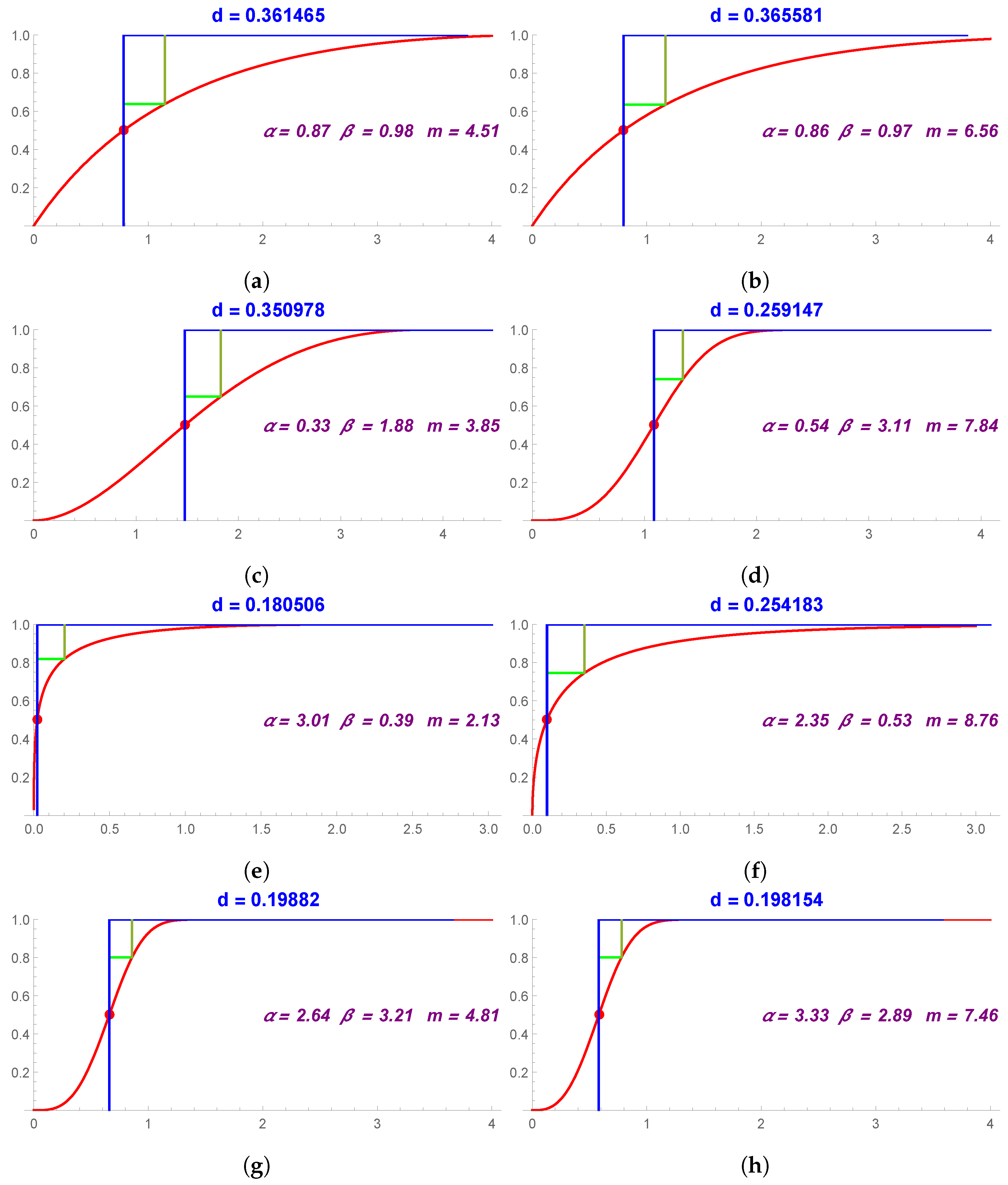
$3.33$	$2.89$	$7.46$	$0.174810$	$0.198154$	$0.304879$	(h)

we present several computational examples to show behavior of the Omega CDF function $F(t;\alpha ,\beta ,m)$ with different values of parameters $\alpha$, $\beta$ and m. We use Theorem 2 for computation of values of upper and lower estimates $d_l$ and $d_r$. It can be seen that the proven bottom estimates for the value of Hausdorff distance d is reliable in approximation of shifted Heaviside function $h_{t_0}\left(t\right)$ and the Omega CDF function $F(t;\alpha ,\beta ,m)$. Graphical representation in Figure 4 shows that the important characteristic “saturation” is faster.

4. Conclusions

Comparatively, the new four-parameter the Pliant probability distribution function can be considered as a generalization of the Epsilon and the Omega distribution. Moreover, it can be viewed as an alternative to some classical probability distributions like Weibull, Exponential, Logistic and Standard Normal distributions. The versatility properties of this probability function lay in the basics of application in different fields of science and modeling problems. The main task in this work is connected to the approximation of the Heaviside function by the Pliant CDF function about the Hausdorff metric. Besides, we present an investigation for the Omega probability distribution. In the presented article we prove upper and lower estimates for the searching Hausdorff approximation that in practice can be used as a possible additional criterion in the exploration of the characteristic “saturation”. For the purpose of this work, a simple dynamic software module is developed and some numerical examples are presented. An example with real data of operating hours between successive failure times of air conditioning systems on Boeing airplanes is considered.

References

- Chen, Z.; Cao, F. The approximation operators with sigmoidal functions. Comput. Math. Appl. 2009, 58, 758–765. [Google Scholar] [CrossRef] [Green Version]
- Kyurkchiev, N.; Markov, S. On the hausdorff distance between the Heaviside step function and Verhulst logistic function. J. Math. Chem. 2016, 54, 109–119. [Google Scholar] [CrossRef]
- Kyukchiev, N.; Iliev, A.; Rahnev, A. A new class of activation functions based on the correcting amendments of Gompertz-Makeham type. Dyn. Syst. Appl. 2019, 28, 243–257. [Google Scholar] [CrossRef] [Green Version]
- Kyurkchiev, N.; Nikolov, G. Comments on some new classes of sigmoidal and activation functions. Applications. Dyn. Syst. Appl. 2019, 28, 789–808. [Google Scholar] [CrossRef]
- Kyurkchiev, N. Comments on the Yun’s algebraic activation function. Some extensions in the trigonometric case. Dyn. Syst. Appl. 2019, 28, 533–543. [Google Scholar] [CrossRef]
- Kyurkchiev, N. Some intrinsic properties of Tadmor–Tanner functions: Related problems and possible applications. Mathematics 2020, 8, 1963. [Google Scholar] [CrossRef]
- Markov, S.; Iliev, A.; Rahnev, A.; Kyukchiev, N. A note on the Log-logistic and transmuted Log-logistic models. Some applications. Dyn. Syst. Appl. 2018, 27, 593–607. [Google Scholar] [CrossRef] [Green Version]
- Yun, B.I. A neural network approximation based on a parametric sigmoidal function. Mathematics 2019, 7, 262. [Google Scholar] [CrossRef] [Green Version]
- Iliev, A.; Kyukchiev, N.; Rahnev, A.; Terzieva, T. Some Models in the Theory of Computer Viruses Propagation; LAP LAMBERT Academic Publishing: Saarbrucken, Germany, 2019; ISBN 978-620-0-00826-8. [Google Scholar]
- Kyukchiev, N.; Iliev, A.; Rahnev, A. Some New Logistic Differential Models: Properties and Applications; LAP LAMBERT Academic Publishing: Saarbrucken, Germany, 2019; ISBN 978-620-0-43442-5. [Google Scholar]
- Kyukchiev, N.; Iliev, A.; Rahnev, A. Some Families of Sigmoid Functions: Applications to Growth Theory; LAP LAMBERT Academic Publishing: Saarbrucken, Germany, 2019; ISBN 978-613-9-45608-6. [Google Scholar]
- Kyukchiev, N.; Markov, S. Sigmoid Functions: Some Approximation and Modelling Aspects. Some Moduli in Programming Environment MATHEMATICA; LAP LAMBERT Academic Publishing: Saarbrucken, Germany, 2015; ISBN 978-3-659-76045-7. [Google Scholar]
- Kyukchiev, N.; Iliev, A.; Markov, S. Some Techniques for Recurrence Generating of Activation Functions: Some Modeling and Approximation Aspects; LAP LAMBERT Academic Publishing: Saarbrucken, Germany, 2017; ISBN 978-3-330-33143-3. [Google Scholar]
- Kyukchiev, N.; Iliev, A. Extension of Gompertz-Type Equation in Modern Science: 240 Anniversary of the Birth of B. Gompertz; LAP LAMBERT Academic Publishing: Saarbrucken, Germany, 2018; ISBN 978-613-9-90569-0. [Google Scholar]
- Kyurkchiev, N.; Iliev, A.; Golev, A.; Rahnev, A. Some Non-Standard Models in “Debugging and Test Theory” (Part 4); Plovdiv University Press: Plovdiv, Bulgaria, 2020; ISBN 978-619-2-02584-7. [Google Scholar]
- Kyukchiev, N. Selected Topics in Mathematical Modeling: Some New Trends. Dedicated to Academician Blagovest Sendov (1932–2020); LAP LAMBERT Academic Publishing: Saarbrucken, Germany, 2020; ISBN 978-613-9-45608-6. [Google Scholar]
- Pavlov, N.; Iliev, A.; Rahnev, A.; Kyukchiev, N. Some Software Reliability Models: Approximation and Modeling Aspects; LAP LAMBERT Academic Publishing: Saarbrucken, Germany, 2018; ISBN 978-613-9-82805-0. [Google Scholar]
- Pavlov, N.; Iliev, A.; Rahnev, A.; Kyukchiev, N. Nontrivial Models in Debugging Theory (Part 2); LAP LAMBERT Academic Publishing: Saarbrucken, Germany, 2018; ISBN 978-613-9-87794-2. [Google Scholar]
- Sendov, B.L. Hausdorff approximations. In Mathematics and Its Applications; Springer Science & Business Media: Berlin/Heidelberg, Germany, 1990; Volume 50, pp. 1–367. [Google Scholar] [CrossRef]
- Dombi, J.; Jónás, T.; Toth, Z.E.; Árva, G. The omega probability distribution and its applications in reliability theory. Qual. Reliab. Eng. Int. 2019, 35, 600–626. [Google Scholar] [CrossRef] [Green Version]
- Dombi, J.; Jónás, T. On an alternative to four notable distribution functions with applications in engineering and the business sciences. Acta Polytech. Hung. 2020, 17, 231–252. [Google Scholar] [CrossRef]
- Dombi, J.; Jónás, T. Advances in the theory of probabilistic and fuzzy data scientific methods with applications. In Studies in Computational Intelligence; Springer: Berlin/Heidelberg, Germany, 2021; Volume 814, pp. 1–186. [Google Scholar] [CrossRef]
- Dombi, J.; Jónás, T.; Tóth, Z. The Epsilon probability distribution and its applications in reliability theory. Acta Polytech. Hung. 2018, 15, 197–216. [Google Scholar] [CrossRef]
- Árva, G. Application of Soft-Computing Techniques for Management Purposes. Fuzzy Likert Scales and Describing and Predicting Empirical Failure Rate Time Series. Ph.D Thesis, Budapest University of Technology and Economics, Budapest, Hungary, 2020; pp. 1–176. [Google Scholar]
- Kyukchiev, N. Comments on the epsilon and omega cumulative distributions: “Saturation in the hausdorff sense”. AIP Conf. Proc. 2020. in print. [Google Scholar]
- Proschan, F. Theoretical explanation of observed decreasing failure rate. Technometrics 1963, 5, 375–383. [Google Scholar] [CrossRef]
- Okorie, I.E.; Nadarajah, S. On the omega probability distribution. Qual. Reliab. Eng. Int. 2019, 35, 2045–2050. [Google Scholar] [CrossRef]
Figure 1.
Functions and for , , , .
Figure 2.
A simple module for the computation and visualization of the Hausdorff distance between the Heaviside step function and the Pliant probability distribution function.