Multi-objective Beam-ACO for Maximising Reliability and Minimising Communication Overhead in the Component Deployment Problem


1
School of Information Technology, Deakin University, Geelong 3126, Australia
2
Faculty of Information Technology, Monash University, Melbourne 3800, Australia
*
Author to whom correspondence should be addressed.
Algorithms 2020, 13(10), 252; https://doi.org/10.3390/a13100252
Submission received: 1 July 2020
/
Revised: 24 September 2020
/
Accepted: 29 September 2020
/
Published: 3 October 2020
(This article belongs to the Special Issue Algorithms for Graphs and Networks)
Abstract
:Automated deployment of software components into hardware resources is a highly constrained optimisation problem. Hardware memory limits which components can be deployed into the particular hardware unit. Interacting software components have to be deployed either into the same hardware unit, or connected units. Safety concerns could restrict the deployment of two software components into the same unit. All these constraints hinder the search for high quality solutions that optimise quality attributes, such as reliability and communication overhead. When the optimisation problem is multi-objective, as it is the case when considering reliability and communication overhead, existing methods often fail to produce feasible results. Moreover, this problem can be modelled by bipartite graphs with complicating constraints, but known methods do not scale well under the additional restrictions. In this paper, we develop a novel multi-objective Beam search and ant colony optimisation (Beam-ACO) hybrid method, which uses problem specific bounds derived from communication, co-localisation and memory constraints, to guide the search towards feasibility. We conduct an experimental evaluation on a range of component deployment problem instances with varying levels of difficulty. We find that Beam-ACO guided by the co-localisation constraint is most effective in finding high quality feasible solutions.
1. Introduction
Software component deployment is a relevant optimisation problem in many domains. In the automotive industry, a growing number of functionalities have to be implemented as software programs and deployed to the hardware infrastructure of a car. The number of potential assignments between software components and hardware units is restricted by a number of hard constraints. Some software requires access to sensors which mandates its positioning on a host residing on the same bus, others cannot be located on the same hardware for safety reasons.
Component deployment optimisation has to fulfill multiple goals, such as reliability, cost, safety, and performance, which can be conflicting, hence the problem is modeled as a multi-objective optimisation problem. Previous approaches to multi-objective models of the automotive component deployment problem comprise bi- and tri-objective formulations. Multi Objective Genetic Algorithm (MOGA) [1], Non-dominated Sorting Genetic Algorithm II (NSGA-II) [2], and Population-Ant Colony Optimisation (P-ACO) [3] were compared on these formulations which resulted in P-ACO outperforming NSGA-II [4]. P-ACO also outperformed MOGA when few iterations were used but not when the algorithm was run for longer, which indicates the slow convergence of MOGA and its ability to escape suboptimal local optima. While these methods have shown to produce good results in the multi-objective setting of the software component deployment problem, their ability to handle constraints is not investigated.
Ant Colony System (ACS) is a method based on the foraging behaviour of ants. Solutions to a problem are constructed by adding components to a partial solution, incrementally. The solutions space of ACS can be viewed as a tree and each component added to the partial solution is a new level of the tree. A similar tree search method is Beam Search which uses a ‘goodness’ estimate at each level of the search tree when constructing solutions. Blum created a hybrid, Beam Ant Colony Optimisation (BACO) that is proven to be more effective than either approach individually on constrained problems [5,6]. For example, experiments on the open shop scheduling problem concluded that BACO outperforms ACO on the vast majority of benchmark instances [5].
A recent application of ACS has found good solutions to a single-objective formulation of the reliability aspect of the component deployment problem [7]. Here, we consider a dual-objective version of the problem where the aim is to maximise reliability and minimise communication overhead. We investigate the efficacy of Beam Ant Colony System (BACS) on this multi-objective version of the problem and determine which problem characteristics lead to the most effective BACS implementation.
To this end, we develop three variants of BACS with problem specific bounds which guide the search to feasible regions. This enables the algorithms to overcome the barriers imposed by hard constraints, which often prohibit finding feasible solutions. The algorithms are compared against ACS and BACS with stochastic sampling. The experimental evaluation conducted on software component deployment problems of various degrees of constrainedness demonstrate the effectiveness of the proposed BACS with different bound estimates. An important outcome we observe is that problem specific bounds can be more effective than generic methods for obtaining estimates (e.g., via stochastic sampling). In summary, this paper makes the following two contributions: (a) introduces a new BACS method for the multi-objective component deployment problem, and (b) proposes three approaches for estimating problem specific bounds for the constrained component deployment problem, and identifies the most effective one.
The paper is organised as follows—Section 2 discusses the component deployment problem. Section 3 reviews the associated literature. This is followed by details of the methods implemented for the problem (Section 4). Section 5 discusses the experiments including the problem instances. The results of the experiments are provided in Section 6 where the algorithms’ performance regarding feasibility and solution quality are analysed. Section 7 concludes the paper.
2. The Constrained Multi-Objective Component Deployment Problem
Quality attributes are important concerns when deploying software components into hardware resources, with reliability and communication overhead being two of the most important ones. Reliability estimates the probability that the software system executes without failure, whereas the communication overhead is a measure of how much data communication is occurring between the hardware units.
2.1. Problem Description
A component deployment problem is characterised by a set of software components, , a set of hardware hosts, , and a set of network links, . Each software component , has properties including memory size , computational requirement , and the probability that the system starts from this component. Also, between any pair of components , is the amount of data sent from to , and is the probability that the execution of component terminates with a call to .
Similarly, each hardware host , has its memory capacity, , the processing capacity, , and the unit failure frequency rate of . In addition, every network link connecting a hardware host to has the data transmission rate of and the failure rate of .
Figure 1 represents an instance of the CDP problem. There are seven software components, four hardware units and three network links. The interaction between the software components are shown as arrows. Because of the high-level of interaction between components and , it is preferable that they are both located on hardware unit (note, the memory capacity of the unit cannot be violated). Components and require a high level of communication, but considering the limitations of memory, safety considerations, or co-localisation aspects, they are embedded on separate hardware units. These two components communicate through network link . The contents of hardware units and and a link between them may be duplicated in another location to maximise the reliability of the system.
We can think of the component deployment problem as an assignment problem , where is the set of all assignments, though some of them would not be feasible. In this notation, as is a assignment, is the hardware host that software component will be deployed.
2.2. Reliability Objective
To model the possible states of a software execution system and the probability of transiting from one state to another, a Discrete Time Markov Chain (DTMC) [8] is used. Essentially, the execution begins at an initial state and terminates either with successful completion or failure. Mathematically, a DTMC can be represented as an ordered tuple where, S is a finite set of states, is the initial state, and is the transition probability matrix, where denotes the probability of changing from state s to state . In a DTMC, for all states , which requires that terminal states also have transition probabilities to themselves. In modelling a software system as DTMC, the execution is considered as a path thorough the states of the DYMC.
DTMC models are characterised by the behavioural specifications of a software embedded system such that a vertex represents the execution of one software component and edges denote the transition of execution from one software component to another. Super-initial vertices represent the beginning of execution, and edges are added from these vertices weighted with corresponding execution initialisation probabilities (q). The model presumes that the failure of components occur independently and the reliability of the component is specified by the failure frequency rate , associated with a component functioning correctly:
where is the hardware host where component is allocated, is its failure rate, is component ’s computational requirement expressed in MI (or million instructions) and the instruction-processing capacity of hardware unit expressed in MILPS (million instructions per second). For a communication element, the reliability is computed by the failure rates of the network links and the amount time spent for communication, defined in Equation (2) as a function of the communication link data rates r and data sizes d required for components and to interact.
The expected number of visits of a DTMC node, expressed in Equation (3), with denoting the probability that the execution of a system starts from component , quantifies the expectation of a component being used during a single system execution.
The transition probabilities can be expressed in a matrix form . In similar fashion, the initialization probabilities can be represented by matrix . The expected number of visits for all components can be written as:
Equation (4) can be expressed as:
where I denotes the identity matrix. For a DTMC with absorbing states, the inverse matrix always exists [8], which guaranties the existence of vector V.
The expected number of visits associated with network links is calculated by , where denotes the expected number of occurrences of the transition . To calculate this value, each probabilistic transition in the model is expressed as a tuple of transitions , the first following the original probability and then terminating in one of the states with probability 1. Considering that the execution of a software system is never initiated in a network link and the only predecessor of link is component , thus the expected number of visits of a network bus is equivalent to
The reliability of a deployment architecture can be computed by taking into account the expected number of visits and reliabilities of execution and communication elements:
2.3. Communication Overhead Objective
When Software systems consist of highly constrained hardware and communication resources, it is advisable to limit high frequent transmissions between software components. For this purpose, the communication overhead (CO) objective was proposed, which imposes minimal data communication for system parameters and components. As a network- and deployment-dependent measure, the overall communication overhead of the system is utilised to represent this viewpoint. This measure was initially developed by Medvidovic and Malek [9] and defined as:
where is the component message size, with if , or in the case that no communication between the two components exists, is the communication frequency between and , is the network bandwidth, with if or there is no network connection between and , and is the network delay, with if or there is no network connection between and .
2.4. Constraints
The software deployment problem is highly constrained. In this work, we consider three common constraints that arise when deploying software components into hardware resources. These are communications, co-localisation and memory.
2.4.1. Communication
The communication between software components limits their allocation to disparate hardware units, since a network link is needed between two hosts if two software components must communicate. Hence, if there is a positive transition probability between two software components and , , these two components must be embeded either on the same hardware host or on different hosts that are connected with a network link with a positive data rate, . The ensuing constraint is:
where is a decision variable has value 1 if component is deployed on hardware host ; Otherwise it is 0.
2.4.2. Co-Localisation
These constraints serve two purposes. First, certain components need to be allocated to different hardware units due to safety and reliability considerations. Second, two software components may need to be allocated to the same host since they require a high level of communication between themselves, and bandwidth limitations will not allow them to be allocated to two different hardware units.
2.4.3. Hardware Memory
Each hardware unit has a memory limit or capacity, which needs to be carefully considered when allocating software components to them. The cumulative memory requirements of software components assigned to hardware units thus leads to the following constraint.
2.5. Multi-Objective Formulation
The communication overhead conflicts with the reliability objective because a system is more reliable when the software components are deployed to different hosts. The failure of a host in such a configuration only compromises the functionality of a single component. Co-locating several components on the same hardware unit minimises the communication overhead. In this study, we consider a bi-objective problem with reliability (Equation (7)) as the first and communication (Equation (8)) overhead as the second objective.
2.6. Graph Representation
The allocation of software components to hardware units connected with network links can be represented as bipartite matching (with complicating constraints) [10]. A bipartite graph consists of two sets of vertices, where edges exist between vertices of the two different sets. For component deployment, one set of vertices are the software components and the second set of vertices are hardware units. A solution to the problem is to select a single edge for every software component vertex that maps it to a hardware unit vertex. In addition to the usual constraints (e.g., selecting edges between software components and hardware units) there are relationships within some of the software components themselves and also the hardware units.
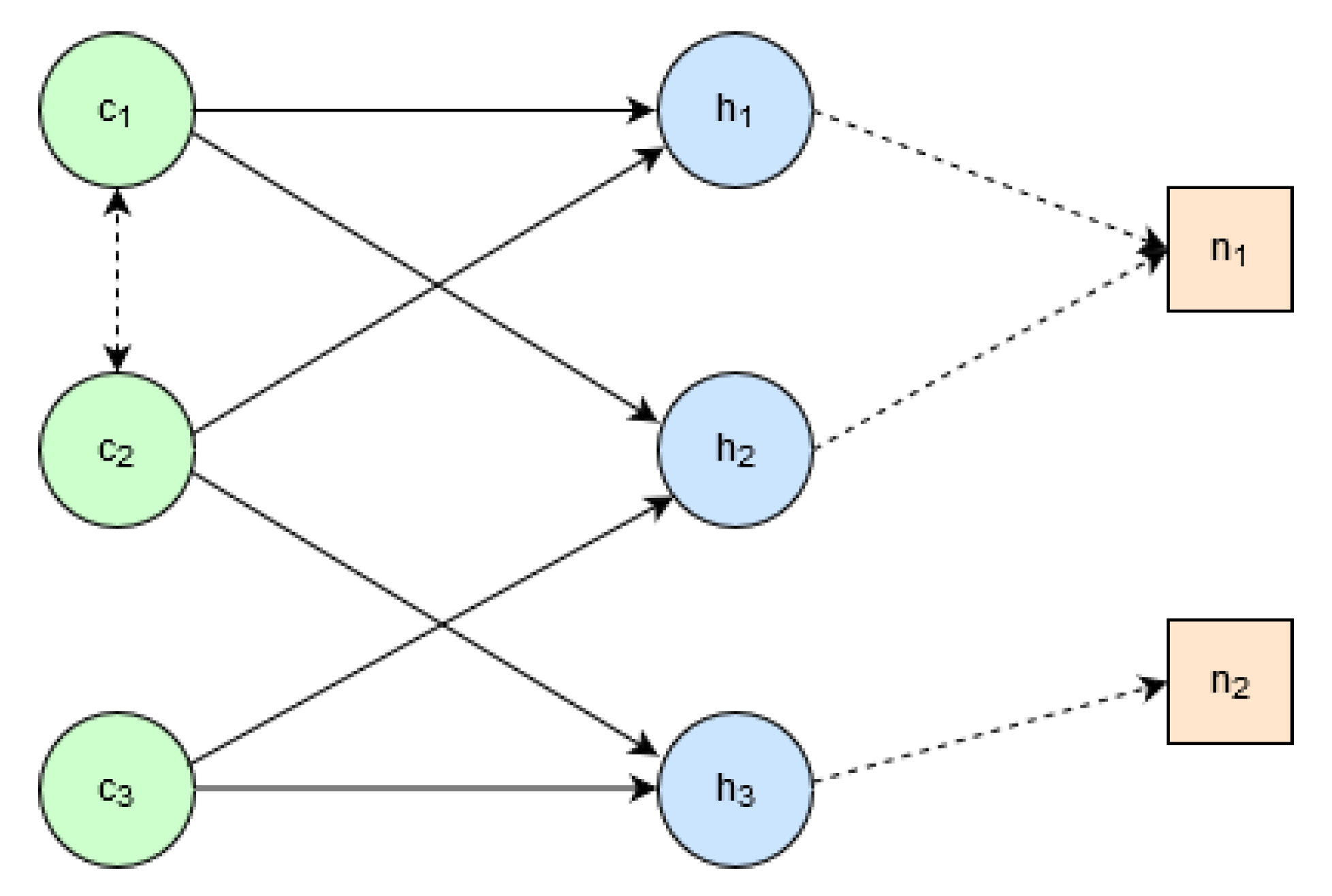
Figure 2 shows a small example problem visualised as a bipartite graph. The software components are , and and hardware units are , and . An edge between a software component and a hardware unit indicates that the software component may be assigned to the corresponding hardware unit (for example, may be assigned to or ). Furthermore, two software components may be linked (indicated by the edge between and ), in which case, they should both be assigned to the same hardware unit or if not, both hardware units they are assigned to must also be linked. For example, if is assigned to , then can be assigned to or since both these hardware units are connected to the link .
While the problem considered in this study has obvious similarities to bipartite matching, extending or adapting existing matching algorithms is not possible in a straightforward manner, since the problem studied here is multi-objective and consists of several complicating constraints.
3. Literature Review
The optimal deployment of software components to distributed hardware units presents itself as a decision making problem in the field of software engineering. The reliability of the deployments is a key criterion for the success of products using those embedded systems. An overarching overview of reliability models used in the deployment of software component is provided by Dimov and Punekkat [11]. In some models the reliability considerations are often the most important aspect [12,13,14], but some authors connect reliability to usage profiles of those systems [14,15] or deduce it from the test coverage of the components [16]. In some cases, the reliability of a software system can be attributed to the component calls or the communication and connections between the components [13,17]. The modelling approaches can also vary, for example, Heydarnoori and Mavaddat [18] model the problem in a distributed system as a multi-way cut problem, in which system reliability is a function of the reliability of the communication links between the interacting components. They approximate the optimal solution in a polynomial-time by deterministic allocation of the components to the hardware units according their connectivity.
The deployment of software components is considered a temporary task in the majority of reliability studies in distributed systems. Assayad, Girault and Kalla [19] solve a bi-objective scheduling problem in which reliability is interpreted as the probability that no software component fails during the execution of the workflow. In a similar work, Kartik and Murthi [20] present a deterministic algorithm which assigns tasks to heterogeneous processing units based on the most-constrained-first criterion: tasks with frequent communication are allocated first. Several mixed integer linear programming (MILP) models have been proposed to the task allocation problem [21,22,23], but none of these have considered reliability of the system.
The study by Hadj-Alouane, Bean and Murti [23] focuses on the task assignment problem in the automotive domain. Their goal was to minimise the cost of installing microcomputers and high-speed or low-speed communication links between the hardware units. They compare their quadratic 0–1 MILP model with a generic algorithm, and find that this algorithm outperforms the MILP by approximately 4% and also uses considerably less CPU time. Moreover, Harris [24] recently provided a inclusive overview of the usage of software components and software engineering in modern vehicles. The author explains the rapid increase in the electronic contents of cars over the past twenty years, facilitated by a shift from dedicated devices and wires to ECUs and Ethernet cables. Climate control, ABS breaks, vision control and wet surface systems have become standard equipment in contemporary cars. In 2002, Leen [25] explained that 23% of the cost of a new car accounted for electronics, and 80% of all innovation is related to the deployment of software components.
Relatively few researchers have engaged with the component deployment problem in automotive systems despite the commercial implications of this problem. Papadopoulos and Grante [26] propose an evolutionary algorithm to select what functionality can be included in a new vehicle model. Their objectives were related to profit and cost considerations, and the deployment of software components to hardware modules focused on reliability. Aleti et al. [27] investigate bi-objective optimisation problem, where the objective criteria were data transmission reliability and communication overhead. On a similar problem, due to a myriad of constraints-including memory restrictions, location and co-location considerations—constructive heuristics [3] and evolutionary approaches [1] were also proposed. Using incremental heuristics on such a heavily constrained problem requires careful constraint manipulation procedures to overcome issues with feasibility. Moser and Mostaghim [28] found that using infeasible solutions in their search led to better solutions overall than eliminating or penalising solutions evolved by NSGA-II [2]. Aleti and Meedeniya [29], also proposed a Bayesian approach adapted to the formulation presented in Reference [27], and showed that they can find better solutions than NSGA-II [2]. Additionally, a formulation of the problem by Meedeniya et al. [30] considers stochastic response times and reliability parameters.
The component deployment problem can also be investigated from a redundancy allocation perspective [31]. In this work, a tri-objective formulation including response time, reliability and cost criteria, is presented and the solution approach is via a genetic algorithm. Sheikhalishahi et al. [32] implement a combination of a genetic algorithm and particle swarm optimisation (PSO) to solve a multi-objective problem which minimises costs, system volume and weights. Liang and Smith [33] adapt an Ant System to also deal with the additional consideration of redundancy allocation. Kumar et al. [34] discuss that redundancy considerations should be focused both at the component level and the module level. They use a hierarchical genetic algorithm to solve their model, and conclude that optimising redundancy at multiple levels provides improved reliability.
4. Methodology
In this section, we discuss in detail the multi-objective ACS and the multi-objective Beam Ant Colony System (BACS) approach we propose in this study. Key to the success of this method, is to keep a pool of solutions in the pareto front, and to execute an ACS or BACS on each of these solutions. Moreover, the choice of bounds is important to guide the BACS search, and hence we discuss different problem specific bounds and also stochastic sampling (a generic estimate proven on a range of problems).
ACS was successfully applied to component deployment in a single-objective setting [7], where a component was chosen randomly, and the host to assign it to was selected based on the pseudo-random proportional rule of ACS. Here, a parameter in the range [0, 1] decides whether to apply the greedy principle or choose the best host according to the distribution given by the pheromone matrix. Pheromones are updated only according to the best solution, and if solutions consist of constraint violations, these do not contribute to reward. The same ACO model is used in the multi-objective approaches that follow.
4.1. Ant Colony System
Algorithm 1 lists a single-objective implementation of BACS [7] with concepts from a multi-objective ACS formulation [35].
| Algorithm 1 Ant Colony System for Multi-objective Component Deployment |
|
An initial solution (), generated by randomly assigning software components to hardware units ( is equivalent to , where the software component is assigned to hardware unit j), is added to set of non-dominated solutions (G). The main algorithm is then run to a time-limit (line 4). Within this loop, an ACS is conducted on each solution in the set of non-dominated solutions, G, and the output solutions of the ACS are considered for inclusion in G (lines 6–8). Thus, the complete set of non-dominated solutions is maintained in G which is output at the end of the algorithm.
The procedure of updating solutions in line 8 works as follows. All solutions in the set I are equal in terms of constraint violations and all of these are non-dominated. These solutions are compared with those in G and the best (least violating) non-dominated solutions after considering both sets are returned.
More formally, a solution is considered an improvement on the existing solutions if it violates fewer constraints than those solutions: , . In this case, all solutions in G are removed and inserted. However, if the violated constraints are equal (, ), then is considered non-dominated in the set G if there is no other solution in the set which is an improvement on when considering both objectives: , .
Algorithm 2 shows the ACS procedure conducted on a single solution . This is now effectively the ACS procedure in the single objective setting, as detailed in Reference [7]. The pheromone trails are initialised and is added to the set of best non-dominated solutions I. The main ACS loop executes between lines 3–11 and the terminating criteria include an iteration limit and a time limit. Within this loop, a number of solutions are constructed and added to the set S (lines 5–7). Each solution is incrementally constructed by assigning software components to hardware units using the pheromone trails.
In particular, the solution construction works as follows. A random number r is chosen in the range , and compared to pre-defined parameter q. If , hardware unit k is chosen with probability:
where is the desirability of selecting hardware unit k for component i. If , hardware unit k is selected such that it has the highest pheromone value:
Moreover, each time a hardware unit is chosen for a software component, the ACS local pheromone update applies:
where is the learning rate and is a small constant that ensures that a hardware unit may always have a chance to be selected for a software component.
In Line 9, the set of non-dominated solutions, I is updated with the best non-dominated solutions considering S and I. The choice of these solutions is carried out exactly as described earlier when discussing Algorithm 1.
| Algorithm 2 ACS() |
|
The pheromone trails are updated in line 10. The component assignments of every solution in I have their values updated in the pheromone matrix in the procedure PheromoneUpdate(I) as , where , is a predefined constant . The violations associated with these solutions are not considered in the pheromone updates. The parameter is set to as determined from initial testing and using Reference [7] as a guide.
Furthermore, every time a hardware unit j is selected for component i, a local pheromone update which is typically used with ACS, is applied as .
4.2. Beam Ant Colony System (BACS)
We now provide details of the multi-objective BACS approach proposed for this study. A key component of the method is to use bounds or estimates to assist in the search. For this purpose, we make use of three different problem specific bounds and also stochastic sampling. This leads to four different variants of multi-objective BACS.
The algorithm presented in the previous section is extended to BACS [5] to solve our highly constrained software component deployment problem. The reasons for this are twofold. Firstly, BACS is known to be better at finding feasible solutions compared to ACS on several problems [36,37,38,39,40]. Given feasibility has already been showed to be problematic for the component deployment problem [7,41], focusing on solving this issue is of high priority.
Secondly, BACS can also be tuned to provide improved solution quality compared to ACS [36,37,38,39,40]. Thus, BACS provides a natural extension to ACS described earlier. Algorithm 1 remains the same. However, line 6 of Algorithm 2, uses a Beam search with pheromones instead. This procedure is presented in Algorithm 3.
| Algorithm 3 BACS |
|
The Beam (B), initially consists of empty solutions. Between lines 4–16, each of these solutions is built incrementally. For each solution in the Beam, solutions for the next software component are generated (lines 7–12). Each of these solutions is unique, each with different assignment of hardware units. Note, the pheromone trails are used in j = selectHU(D,) to bias the selection of the hardware units for each component.
Once all solutions for the components have been determined, the Beam potentially consists of solutions. These have to be restricted to solutions and this is achieved in line 14: Reduce. For each solution, an estimate is computed (discussed next) which gives each solution a rank. From these, the top ranked solutions are selected.
Bound Estimates
In Beam search, when extending a solution with a component, estimates of the ‘goodness’ of the component are critical to finding good areas of a search space. A bound is a value which an optimal solution cannot improve upon. Consider a minimisation problem with optimal solution and lower bound . Then, .
For the problem being considered, a good estimate is one that leads the search towards (1) feasible regions and (2) high quality regions. Problem specific bounds can be used to obtain such estimates. In Algorithm 3, line 14 uses an estimate to reduce the set of solutions to solutions. In this study we explore four different bounds focused on finding feasibility.
- Stochastic sampling: this estimate has been successfully used earlier and often outperforms problem specific bounds [36,37,38,39,40]. The idea implemented here is straightforward. Given a partial solution ( components are assigned), a number of samples are generated by assigning hardware units to the remaining components using the pheromone bias. The best of these samples (considering violations, reliability and communication overhead) is used as the estimate for this solution.
- Communication estimate: given a partial solution ( components are assigned), the remaining software components are assigned hardware units ensuring the communication constraint is always satisfied. This is a greedy selection, and hence only a single solution is generated. Note, the co-localisation and memory constraints may not be satisfied.
- Co-localisation estimate: as with the communication estimate, the software components are assigned hardware units satisfying the co-localisation constraint. As a result of this greedy selection process, the communication and memory constraints may not be satisfied.
- Memory estimate: as with the previous two estimates, remaining software components are assigned ensuring no violation of the memory constraint. Again, since it is a greedy procedure, the communication and co-localisation constraints may not be satisfied.
5. Experiments
In this section, we explain the set-up for the experiments, algorithms and problems. All experiments were conducted on MONARCH, a cluster at Monash University. We applied 5 different algorithms to solve different instances of multi-objective component deployment problem.
5.1. Algorithms
We compare the performance of Ant Colony Systems (ACS) against four different variants of BACS algorithm. The main difference between these variants is in the methodology they use to minimise the amount of constraint violation throughout the construction process of feasible solutions. BACS(Mem) is a variant of BACS implementation that prioritises memory and hence ensure that memory related constraints are always satisfied when building solutions. Similarly, BACS(Col) and BACS(Com) are variants of BACS that try to minimise violations regarding constraints related co-localisation and computational overhead, respectively. Finally, BACS(SS) is the variant of BACS that assigns software components to hardware units using stochastic sampling.
5.2. Problem Instances
The instances used for numerical experiments were created randomly with varying complexity and constrainedness. For each instance, all the parameters including the number of hardware units, software components, network links, and their specifications are generated randomly. We conducted numerical experiments on problems with 15, 33 and 60 hardware units and 23, 34, 47 and 51 software components.
Additionally, the proportion of software components that require the services of each other is expressed as a percentage which can be 10%, 25%, 50%, 75%, and 100%. As an example, the instance H33C47I10 has 33 hardware units, 47 software components, 10% of which interact with each other and require to be deployed either in the same hardware unit or in hardware units that have a network between them. It is important to note that there is no guarantee for a feasible solution for any of the problems.
In our optimisation process, there are two objectives, namely, reliability and communication overhead. However, before optimising these objective, we first minimise the amount of violations over the existing constraints in order to achieve feasibility. As a next step, we maximise reliability and the communication overhead, simultaneously.
To obtain the numerical results, we executed each algorithm 30 times with a 600 s time limit. The results at the end of the time limit are reported and analysed.
6. Results
We present the results by first investigating feasibility and second, solution quality. The emphasis is first on feasibility since if feasible solutions are not found the high values of reliability and communication overhead do not mean much, as the solution can not be implemented in a real scenario.
6.1. Feasibility
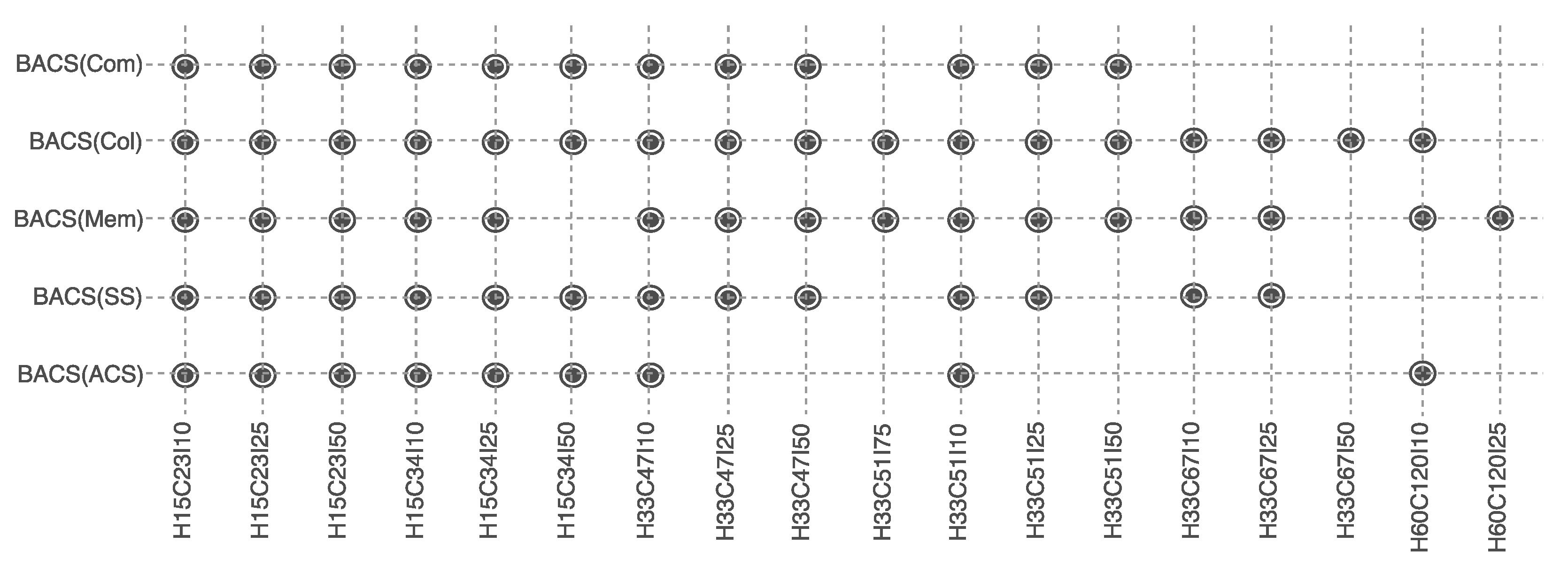
To determine the efficacy of each algorithm on feasibility, we consider two figures (Figure 3 and Figure 4). The first figure demonstrate hardness of individual problems and how well the algorithms perform. The second figure demonstrates feasibility as a proportion of feasible solution found across all instances for each algorithm.
Figure 3 demonstrates the effectiveness of the optimisation schemes in finding feasible solutions for problem instances of different levels of difficulty. A ‘dot’ at the junction of an algorithm and a problem instance indicates that the algorithm successfully finds a feasible non-dominated Pareto solution.
The size of the problem impacts, to some extent, the ability of the algorithms to find feasible solutions. For example, H33C67I25 and H60C120I25 are similar in terms of constraints, but H60C120I25 is larger. As Figure 3 shows, for the larger problem only BACS(Mem) was able to find a feasible solution, whereas the smaller problem was solved to feasibility by three out of five algorithms, all of which use bounds to prune the search space. The figure indicates the relative hardness of each problem.
Out of the five optimisation schemes, BACS(Col) has the highest rate of success by solving 94% of problems to feasibility, followed by BASC(Mem) which has a success rate of 89%. This method considers co-location as the hardest constraint to satisfy, and aims at minimising co-location related constraint violations. Once the co-location constraint is satisfied, the other constraints do not pose any difficulty in finding feasible solutions. It is only in the largest problem H60C120I25 that BACS(Col) is not able to find feasible solution. Nevertheless, these results indicate that using co-location related bounds to guide the search algorithm results in finding feasibility.
Prioritising the communication constraint, on the other hand, is not beneficial. In this case, the optimisation algorithm may attempt to allocate all interacting components into the same hardware unit, which violates the memory and co-localisation constraints. This is clearly not an effective strategy and should not be used to optimise highly constrained component deployment problems.
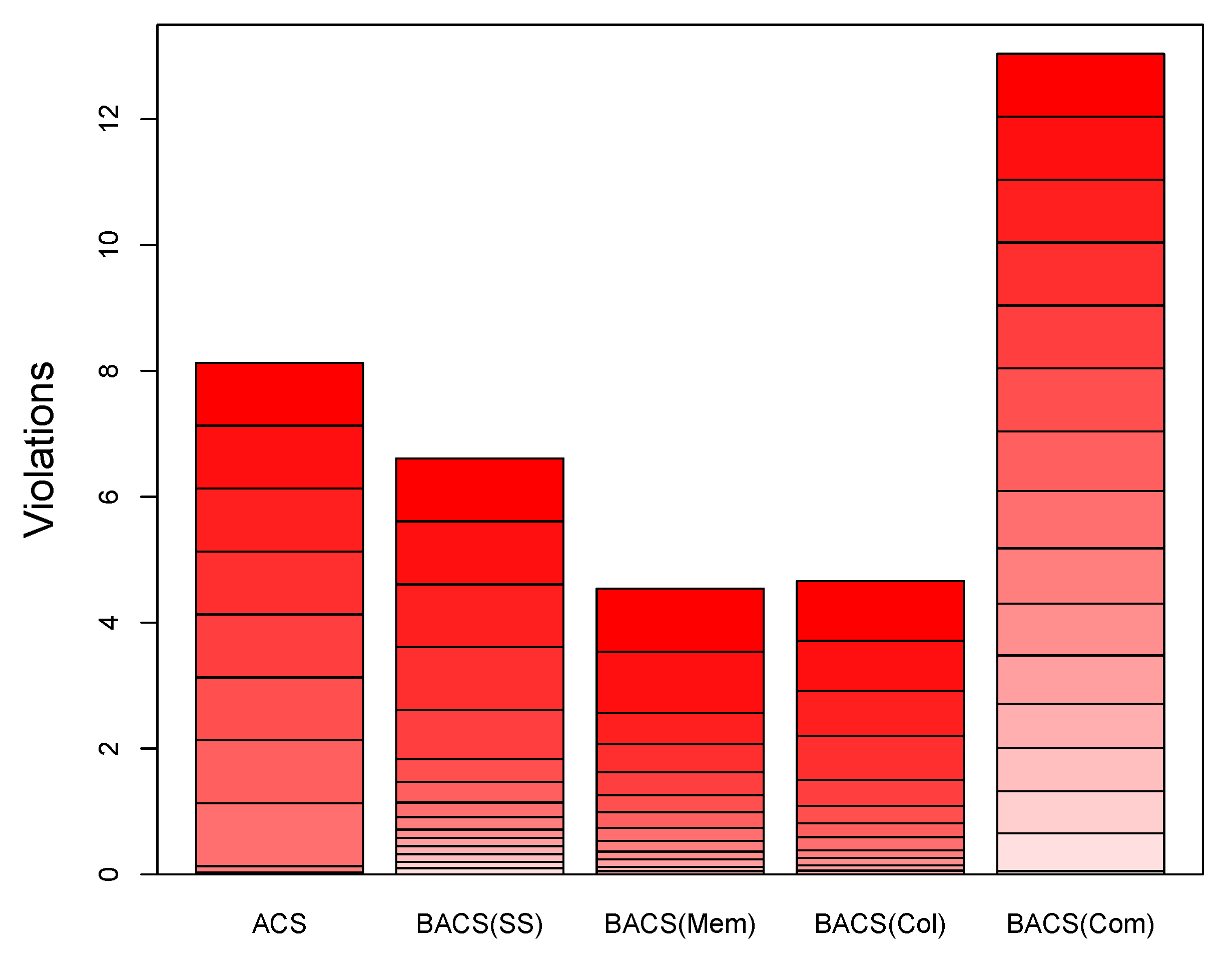
Figure 4 summarises the results that focus on constraint satisfaction by showing the number of violations across all problem instances for each optimisation scheme. We see that three out of the four variants of BACS (enforcing memory, colocalisation or via stochastic sampling) are more effective in finding feasibility compared to ACS. Similar to the results shown in Figure 3, the BACS version that prioritises the communication-related constraints performs worse than ACS.
There are a few reasons why ACS is outperformed by the three BACS versions. First, the bound estimates have proven useful in guiding the algorithm towards feasibility. Communication bounds, however, are not as effective in achieving feasibility, due to the interaction of this constraint with the other two constraints. As we noted above, prioritising communication constraint leads to high violations in terms of the other two constraints, preventing the algorithm from finding feasible solutions.
Secondly, the different solution construction mechanism of both Beam search and ACS which are combined into the BACS method are significantly different and complement each other. At each solution construction step, Beam search enforces the choice of a new solution component. Especially, when the method is searching close to feasibility, this can result in moving to feasible regions. ACS, on the other hand, can repeatedly construct the same solution and can be useful especially when the algorithm is close to convergence.
6.2. Solution Quality
The hypervolume indicator [42] is used to measure the performance of multi-objective optimisation methods. The metric provides the volume, or area in 2-dimensional space, of the objective subspace that is dominated by the Pareto front.
Consider a multi-objective optimisation problem with two criteria similar to the problem we are solving in this paper. Mathematically, consider that we want to minimise and . The (local) optimal solutions, Pareto optima, are the minimal elements regarding a weak dominance relation. In this setting, the Pareto front is the image of the Pareto solution set under the mapping . Our aim is to evaluate the set of Pareto optima using hypervolumes which measures the quality of a solution set. The hypervolume indicator, , for a solution set and a reference set is defined as where , is the set of points in that are enclosed by the Pareto front and the reference set and is the Lebesgue measure to calculate the volume [43]. The maximum hypervolume value is achieved if for each , the solution set A contains at least a point so that . In other words, the Pareto front is contained in the image of A under [44].
Figure 5 provides an overview of the performance of all algorithms in terms of hypervolume values achieved over the 30 runs shown as boxplots for each problem instance. The components of Figure 5 are laid out in a way that from left to right and from top to bottom the size of problems is increasing. A larger hypervolume value indicates a better solution. Note that in order to compare reliability and communication overhead on the same scale, the communication overhead was normalised.
It can be seen that for the smaller problems, ACS is more effective than BACS. Moving from top-left to the bottom-right of Figure 5, the complexity (and size) of the instances increases and finding good quality and feasible solutions is harder. We see that as the problems become more complicated, the BACS variants obtain larger hypervolumes. In particular, toward the bottom of the Figure, BACS(Mem) shows its superiority in obtaining better quality solutions for the difficult problem instances.
6.3. Summary of Results
Table 1 summarises the feasibility as success rate and solution quality as the mean objective value over the 30 runs and 18 problem instances.
The first row (Success Rate) shows the average success rate, or feasibility, across all instances for all algorithms. This is calculated as the number of times a solution was found by the algorithm relative to the total number of runs. Similarly, the second and third rows (Mean Reliability, Mean Com. Overhead) show the average reliability and communication overhead, respectively, across all instances (where feasibility was found) for each algorithm. We see here that BACS (Col) is the best performing algorithm considering all measures, hence we conclude that using co-location bounds to guide the optimisation method towards feasible regions is the most effective method in finding not only feasible but also high-quality solutions.
Due to the stochastic behavior of the algorithms, we conducted 30 runs per algorithm, which showed variability between runs in the results. Hence, the discrepancies are analysed for statistical significance considering the reliability and communication overhead criteria and the levels of violations seen. We performed an unpaired t-test on the means for all pairs of algorithms regarding reliability, communication overhead and the total number of violations.
Let denote the difference between average reliability obtained from alg1 and alg2. The following competing hypotheses are tested against each other.
The p-value of each test is obtained from the mean, the standard deviation, and the number of successful cases seen in each algorithm. The following matrix represents the p-values for each test given the 0.05 significance level.
The first row of the matrix, clearly, shows that all versions of BACS are statistically different from ACS.
The same argument is valid in comparing the performance of different algorithms considering the number of violations. In particular, the following matrix is the result of a pair-wise test of different algorithms regarding violations.
The matrices of p-values, in particular the first rows, provide strong evidence of significant differences between the algorithms, hence we conclude that the superior performance of BACS is statistically significant.
7. Conclusions
This study investigates Beam Ant Colony System (BACS) for solving the highly constrained multi-objective (reliability and communication overhead) component deployment problem. Four variants of BACS are investigated where each variant is different with respect to the estimates used to guide the search towards feasible regions. We find that three of the four BACS variants are more effective than ACS with respect to feasibility. These are the variants that are based on stochastic sampling, respecting memory constraints and enforcing co-localisation constraints.
The variant of BACS that enforces the communication constraints struggles with feasibility. Regarding solution quality, we find that ACS is effective on small problems when feasibility is found. With increasing problem size, the BACS variants are more effective, and in particular, BACS(Mem) (respecting memory constraints) is the best performing algorithm in large problem. On the other hand, BACS(Col) which prioritises co-localisation constraint is the overall best performing method, both in terms of feasibility and solutions quality hence we recommend it for the highly constrained multi-objective component deployment problem.
In the future, we plan to solve more difficult instances with a larger number of software components and hardware units. In order to do this effectively, we will consider parallel implementations of our methods via multi-core shared memory and message passing interface (e.g., using approaches such as that of References [45,46,47]. Furthermore, approaches tailored for multi-objective problems which deal with hard constraints effectively, can be of great potential [48,49,50].
Author Contributions
D.T. developed the algorithms and ensuing implementations and led the writing of the manuscript. A.N. carried out the data analysis, prepared the visualisation, and wrote the experiment and results section. A.A. provided the motivation for the problem, developed a problem generator, ideas for the algorithms, and wrote parts of the manuscript. All authors have read and agreed to the published version of the manuscript.
Funding
This research received no external funding.
Conflicts of Interest
The authors declare no conflict of interest.
References
- Fonseca, C.M.; Fleming, P.J. Genetic Algorithms for Multiobjective Optimization: Formulation, Discussion and Generalization. In Proceedings of the 5th International Conference on Genetic Algorithms, Champaign, IL, USA, 17–22 July 1993; Volume 93, pp. 416–423. [Google Scholar]
- Deb, K.; Pratap, A.; Agarwal, S.; Meyarivan, T. A Fast Elitist Multi-Objective Genetic Algorithm: NSGA-II. IEEE Trans. Evol. Comput. 2000, 6, 182–197. [Google Scholar] [CrossRef] [Green Version]
- Guntsch, M.; Middendorf, M. Solving Multi-criteria Optimization Problems with Population-Based ACO. In Proceedings of the Evolutionary Multi-Criterion Optimization, Second International Conference, EMO 2003, Faro, Portugal, 8–11 April 2003; Springer: Berlin, Germany, 2003; pp. 464–478. [Google Scholar]
- Moser, I.; Montgomery, J. Population-ACO for the Automotive Deployment Problem. In Proceedings of the 13th Annual Conference on Genetic and Evolutionary Computation, GECCO’11, Dublin, Ireland, 12–16 July 2011; ACM: New York, NY, USA, 2011; pp. 777–784. [Google Scholar]
- Blum, C. Beam-ACO: Hybridizing Ant Colony Optimization with Beam Search: An Application to Open Shop Scheduling. Comput. Oper. Res. 2005, 32, 1565–1591. [Google Scholar] [CrossRef]
- Blum, C. Beam-ACO for Simple Assembly Line Balancing. INFORMS J. Comput. 2008, 20, 618–627. [Google Scholar] [CrossRef]
- Thiruvady, D.; Moser, I.; Aleti, A.; Nazari, A. Constraint Programming and Ant Colony System for the Component Deployment Problem. Procedia Comput. Sci. 2014, 29, 1937–1947. [Google Scholar] [CrossRef]
- Trivedi, K. Probability and Statistics with Reliability, Queuing and Computer Science Applications; Wiley: New Delhi, India, 2009; pp. 337–392. [Google Scholar]
- Medvidovic, N.; Malek, S. Software deployment architecture and quality-of-service in pervasive environments. In Proceedings of the Workshop on the Engineering of Software Services for Pervasive Environements, ESSPE, Dubrovnik, Croatia, 4 September 2007; ACM: New York, NY, USA, 2007; pp. 47–51. [Google Scholar]
- Manlove, D. Algorithmics of Matching Under Preferences; World Scientific: Singapore, 2013. [Google Scholar]
- Dimov, A.; Punnekkat, S. On the Estimation of Software Reliability of Component-Based Dependable Distributed Systems. In Quality of Software Architectures and Software Quality; Reussner, R., Mayer, J., Stafford, J., Overhage, S., Becker, S., Schroeder, P., Eds.; Lecture Notes in Computer Science; Springer: Berlin/Heidelberg, Germany, 2005; Volume 3712, pp. 171–187. [Google Scholar]
- Cheung, R.C. A User-Oriented Software Reliability Model. IEEE Trans. Softw. Eng. 1980, 6, 118–125. [Google Scholar] [CrossRef]
- Krishnamurthy, S.; Mathur, A. On The Estimation of Reliability of A Software System Using Reliabilities of Its Components. Softw. Reliab. Eng. Int. Symp. 1997, 146–155. [Google Scholar] [CrossRef]
- Reussner, R.; Schmidt, H.W.; Poernomo, I. Reliability prediction for component-based software architectures. J. Syst. Softw. 2003, 66, 241–252. [Google Scholar] [CrossRef]
- Hamlet, D.; Mason, D.; Woit, D. Theory of Software Reliability Based on Components. In Proceedings of the 23rd International Conference on Software Engineering, ICSE ’01, Toronto, ON, Canada, 19 May 2001; pp. 361–370. [Google Scholar]
- Gokhale, S.; Philip, T.; Marinos, P.; Trivedi, K. Unification of finite failure non-homogeneous Poisson process models through test coverage. In Proceedings of the Seventh International Symposium on Software Reliability Engineering, White Plains, NY, USA, 30 October–2 November 1996; pp. 299–307. [Google Scholar]
- Singh, H.; Cortellessa, V.; Cukic, B.; Gunel, E.; Bharadwaj, V. A Bayesian Approach to Reliability Prediction and Assessment of Component Based Systems. In Proceedings of the 12th International Symposium on Software Reliability Engineering, Hong Kong, China, 27–30 November 2001; pp. 12–21. [Google Scholar]
- Heydarnoori, A.; Mavaddat, F. Reliable Deployment of Component-based Applications into Distributed Environments. In Proceedings of the Third International Conference on Information Technology: New Generations (ITNG’06), Las Vegas, NV, USA, 10–12 April 2006. [Google Scholar]
- Assayad, I.; Girault, A.; Kalla, H. A Bi-Criteria Scheduling Heuristic for Distributed Embedded Systems under Reliability and Real-Time Constraints. In Proceedings of the Dependable Systems and Networks (DSN’04), IEEE Computer Society, Florence, Italy, 28 June–1 July 2004; pp. 347–356. [Google Scholar]
- Kartik, S.; Murthy, C. Task allocation algorithms for maximizing reliability of distributed computing systems. IEEE Trans. Comput. 1997, 46, 719–724. [Google Scholar] [CrossRef]
- Bowen, N.; Nikolaou, C.; Ghafoor, A. On the assignment problem of arbitrary process systems to heterogeneous distributed computer systems. IEEE Trans. Comput. 1992, 41, 257–273. [Google Scholar] [CrossRef]
- Ernst, A.; Jiang, H.; Krishnamoorthy, M. Exact Solutions to Task Allocation Problems. Manag. Sci. 2006, 52, 1634–1646. [Google Scholar] [CrossRef] [Green Version]
- Hadj-Alouane, A.B.; Bean, J.; Murty, K. A hybrid genetic/optimisation algorithm for a task allocation problem. J. Sched. 1999, 2, 189–201. [Google Scholar] [CrossRef]
- Harris, I. Embedded Software for Automotive Applications. In Software Engineering for Embedded Systems; Oshana, R., Kraeling, M., Eds.; Newnes: Newton, MA, USA, 2013; pp. 767–816. [Google Scholar]
- Leen, G. Expanding Automotive Electronic Systems. IEEE Comput. 2002, 35, 88–93. [Google Scholar] [CrossRef]
- Papadopoulos, Y.; Grante, C. Evolving car designs using model-based automated safety analysis and optimisation techniques. J. Syst. Softw. 2005, 76, 77–89. [Google Scholar] [CrossRef]
- Aleti, A.; Grunske, L.; Meedeniya, I.; Moser, I. Let the ants deploy your software—An ACO based deployment optimisation strategy. In Proceedings of the International Conference on Automated Software Engineering (ASE’09), IEEE Computer Society, Auckland, New Zealand, 16–20 November 2009; pp. 505–509. [Google Scholar]
- Moser, I.; Mostaghim, S. The automotive deployment problem: A practical application for constrained multiobjective evolutionary optimisation. In Proceedings of the IEEE Congress on Evolutionary Computation, Barcelona, Spain, 18–23 July 2010; pp. 1–8. [Google Scholar]
- Aleti, A.; Meedeniya, I. Component Deployment Optimisation with Bayesian Learning. In Proceedings of the International ACM Sigsoft Symposium on Component Based Software Engineering, Boulder, CO, USA, 20–24 June 2011; ACM: New York, NY, USA, 2011; pp. 11–20. [Google Scholar]
- Meedeniya, I.; Aleti, A.; Avazpour, I.; Amin, A. Robust ArcheOpterix: Architecture optimization of embedded systems under uncertainty. In Proceedings of the 2012 Second International Workshop on Software Engineering for Embedded Systems (SEES), Zurich, Switzerland, 9 June 2012; pp. 23–29. [Google Scholar]
- Aleti, A. Designing automotive embedded systems with adaptive genetic algorithms. Autom. Softw. Eng. 2015, 22, 199–240. [Google Scholar] [CrossRef]
- Sheikhalishahi, M.; Ebrahimipour, V.; Shiri, H.; Zaman, H.; Jeihoonian, M. A hybrid GA-PSO approach for reliability optimization in redundancy allocation problem. Int. J. Adv. Manuf. Technol. 2013, 68, 317–338. [Google Scholar] [CrossRef]
- Liang, Y.C.; Smith, A. An ant system approach to redundancy allocation. In Proceedings of the 1999 Congress on Evolutionary Computation-CEC99, Washington, DC, USA, 6–9 July 1999; Volume 2, pp. 1478–1484. [Google Scholar]
- Kumar, R.; Izui, K.; Yoshimura, M.; Nishiwaki, S. Optimal Multilevel Redundancy Allocation in Series and Series-parallel Systems. Comput. Ind. Eng. 2009, 57, 169–180. [Google Scholar] [CrossRef]
- López-Ibáñez, M.; Stützle, T. The Automatic Design of Multi-Objective Ant Colony Optimization Algorithms. IEEE Trans. Evol. Comput. 2012, 16, 861–875. [Google Scholar] [CrossRef] [Green Version]
- López-Ibáñez, M.; Blum, C. Beam-ACO Based on Stochastic Sampling: A Case Study on the TSP with Time Windows; Technical Report LSI-08-28; Department LSI, Univeristat Politècnica de Catalunya: Barcelona, Spain, 2008. [Google Scholar]
- López-Ibáñez, M.; Blum, C.; Thiruvady, D.; Ernst, A.T.; Meyer, B. Beam-ACO Based on Stochastic Sampling for Makespan Optimization Concerning the TSP with Time Windows. Lect. Notes Comput. Sci. 2009, 5482, 97–108. [Google Scholar]
- Thiruvady, D.; Blum, C.; Meyer, B.; Ernst, A.T. Hybridizing Beam-ACO with Constraint Programming for Single Machine Job Scheduling. Lect. Notes Comput. Sci. 2009, 5818, 30–44. [Google Scholar]
- Thiruvady, D.; Singh, G.; Ernst, A.T.; Meyer, B. Constraint-based ACO for a Shared Resource Constrained Scheduling Problem. Int. J. Prod. Econ. 2012, 141, 230–242. [Google Scholar] [CrossRef]
- Thiruvady, D.R.; Meyer, B.; Ernst, A. Car Sequencing with Constraint-based ACO. In Proceedings of the 13th Annual Conference on Genetic and Evolutionary Computation, GECCO’11, Dublin, Ireland, 12–16 July 2011; ACM: New York, NY, USA, 2011; pp. 163–170. [Google Scholar]
- Nazari, A.; Thiruvady, D.; Aleti, A.; Moser, I. A mixed integer linear programming model for reliability optimisation in the component deployment problem. J. Oper. Res. Soc. 2016, 67, 1050–1060. [Google Scholar] [CrossRef]
- Zitzler, E.; Thiele, L. Multiobjective optimization using evolutionary algorithms — A comparative case study. In Parallel Problem Solving from Nature—PPSN V, Proceedings of the 5th International Conference, Amsterdam, The Netherlands, 27–30 September 1998; Springer: Berlin/Heidelberg, Germany, 1998; pp. 292–301. [Google Scholar]
- Auger, A.; Bader, J.; Brockhoff, D.; Zitzler, E. Theory of the Hypervolume Indicator: Optimal μ-distributions and the Choice of the Reference Point. In Proceedings of the Tenth ACM SIGEVO Workshop on Foundations of Genetic Algorithms, FOGA ’09, Orlando, FL, USA, 9–11 January 2009; ACM: New York, NY, USA, 2009; pp. 87–102. [Google Scholar]
- Fleischer, M. The Measure of Pareto Optima Applications to Multi-objective Metaheuristics. In Evolutionary Multi-Criterion Optimization, Proceedings of the Second International Conference, EMO 2003, Faro, Portugal, 8–11 April 2003; Springer: Berlin/Heidelberg, Germany, 2003; pp. 519–533. [Google Scholar]
- Brent, O.; Thiruvady, D.; Gómez-Iglesias, A.; Garcia-Flores, R. A Parallel Lagrangian-ACO Heuristic for Project Scheduling. In Proceedings of the 2014 IEEE Congress on Evolutionary Computation, Beijing, China, 6–11 July 2014; pp. 2985–2991. [Google Scholar]
- Cohen, D.; Gómez-Iglesias, A.; Thiruvady, D.; Ernst, A.T. Resource Constrained Job Scheduling with Parallel Constraint-Based ACO. In Proceedings of the ACALCI 2017—Artificial Life and Computational Intelligence, Geelong, Australia, 31 January–2 February 2017; Wagner, M., Li, X., Hendtlass, T., Eds.; Lecture Notes in Computer Science. Springer International Publishing: New York, NY, USA, 2017; Volume 10142, pp. 266–278. [Google Scholar]
- Thiruvady, D.; Ernst, A.T.; Singh, G. Parallel Ant Colony Optimization for Resource Constrained Job Scheduling. Ann. Oper. Res. 2016, 242, 355–372. [Google Scholar] [CrossRef]
- Li, X.; Li, M.; Yin, M. Multiobjective ranking binary artificial bee colony for gene selection problems using microarray datasets. IEEE/CAA J. Autom. Sin. 2016. [Google Scholar] [CrossRef]
- Wang, Y.; Liu, H.; Zheng, W.; Xia, Y.; Li, Y.; Chen, P.; Guo, K.; Xie, H. Multi-Objective Workflow Scheduling With Deep-Q-Network-Based Multi-Agent Reinforcement Learning. IEEE Access 2019, 7, 39974–39982. [Google Scholar] [CrossRef]
- Guo, X.; Zhou, M.; Liu, S.; Qi, L. Lexicographic Multiobjective Scatter Search for the Optimization of Sequence-Dependent Selective Disassembly Subject to Multiresource Constraints. IEEE Trans. Cybern. 2020, 50, 3307–3317. [Google Scholar] [CrossRef]
Figure 1.
An example of the component deployment problem. The hardware units.

Figure 2.
A bipartite graph representation of the component deployment problem.

Figure 3.
The performance of the algorithms on all instances in terms of feasibility. A dot indicates that an algorithm has identified a feasible solution for an instance.
Figure 3.
The performance of the algorithms on all instances in terms of feasibility. A dot indicates that an algorithm has identified a feasible solution for an instance.

Figure 4.
Feasibility violation of algorithms on different constraints.

Figure 5.
The 30 hypervolume values of each optimisation scheme on the instances where solutions are found by all algorithms. SS = BACS (SS), Mem = BACS (Mem), Col = BASC (Col), and Com = BACS (Com).
Figure 5.
The 30 hypervolume values of each optimisation scheme on the instances where solutions are found by all algorithms. SS = BACS (SS), Mem = BACS (Mem), Col = BASC (Col), and Com = BACS (Com).


Table 1.
A summary of the performance of the algorithms across all instances. The results highlighted in boldface are statistically significant.
Table 1.
A summary of the performance of the algorithms across all instances. The results highlighted in boldface are statistically significant.
| ACS | BACS (SS) | BACS (Mem) | BACS (Col) | BACS (Com) | |
|---|---|---|---|---|---|
| Success Rate | 0.5 | 0.72 | 0.89 | 0.94 | 0.61 |
| Mean Reliability | 0.44 | 0.44 | 0.44 | 0.56 | 0.5 |
| Mean Com. Overhead | 0.62 | 0.62 | 0.71 | 0.92 | 0.86 |
© 2020 by the authors. Licensee MDPI, Basel, Switzerland. This article is an open access article distributed under the terms and conditions of the Creative Commons Attribution (CC BY) license (http://creativecommons.org/licenses/by/4.0/).
Share and Cite
MDPI and ACS Style
Thiruvady, D.; Nazari, A.; Aleti, A. Multi-objective Beam-ACO for Maximising Reliability and Minimising Communication Overhead in the Component Deployment Problem. Algorithms 2020, 13, 252. https://doi.org/10.3390/a13100252
AMA Style
Thiruvady D, Nazari A, Aleti A. Multi-objective Beam-ACO for Maximising Reliability and Minimising Communication Overhead in the Component Deployment Problem. Algorithms. 2020; 13(10):252. https://doi.org/10.3390/a13100252
Chicago/Turabian StyleThiruvady, Dhananjay, Asef Nazari, and Aldeida Aleti. 2020. "Multi-objective Beam-ACO for Maximising Reliability and Minimising Communication Overhead in the Component Deployment Problem" Algorithms 13, no. 10: 252. https://doi.org/10.3390/a13100252
Note that from the first issue of 2016, this journal uses article numbers instead of page numbers. See further details here.