A Numerical Approach for the Filtered Generalized Čech Complex

Abstract

In this paper, we present an algorithm to compute the filtered generalized Čech complex for a finite collection of disks in the plane, which do not necessarily have the same radius. The key step behind the algorithm is to calculate the minimum scale factor needed to ensure rescaled disks have a nonempty intersection, through a numerical approach, whose convergence is guaranteed by a generalization of the well-known Vietoris–Rips Lemma, which we also prove in an alternative way, using elementary geometric arguments. We give an algorithm for computing the 2-dimensional filtered generalized Čech complex of a finite collection of d-dimensional disks in ${\mathbb{R}}^d$, and we show the performance of our algorithm.

1. Introduction

Recently, in the study of data point clouds from a topological approach (cf. [1,2,3,4,5]), the need to develop algorithms to construct different simplicial structures has arisen, such as the Vietoris–Rips complex, the Čech complex, the piecewise linear lower star complex, etc. (cf. [6,7]).

Of particular interest to us is the generalized Čech complex structure, whereas the standard Čech complex is induced by the intersection of a collection of disks with fixed radius, the generalized version admits different radii (see [8]); when radii are rescaled, using the same scale factor each time, the corresponding simplicial complexes forms the filtered generalized Čech complex.

There exist efficient algorithms to calculate the standard Čech complex (see, e.g., in [9]), and software currently available to obtain the associated filtration (cf. [10,11]); also, in [12] the authors propose an algorithm to approximate the Čech filtration. On the other hand, we can find algorithms to calculate the generalized Čech complex (see, e.g., in [8]); however, as far as we know, there are neither algorithms nor software to provide the filtered generalized Čech complex. In the present work, we show an algorithm to compute the filtered generalized Čech complex for a finite collection of disks, specifically, in the plane. Actually, we also show an algorithm to build up to the 2-dimensional filtered generalized structure (or 2-skeleton), for higher-dimensional disk systems, which many applications only require, as we can see in [13,14,15,16,17].

The key step behind these proposed algorithms, is to calculate the minimum scale factor (called Čech scale) needed to ensure that the rescaled disks have a nonempty intersection; the generalized Vietoris–Rips lemma over multiple radii will allow us to calculate these scales numerically.

We must emphasize that our main algorithm (Algorithm 3) is only generalizable to higher-dimensional disk systems to obtain the 2-dimensional filtered generalized Čech structure, as we show as an application. Additionally, we show how our algorithm yields the minimal enclosing ball for a finite set of points in the plane.

This paper is organized as follows. In Section 2, we introduce basic notions and notation which will be used throughout the paper. We define the Vietoris–Rips system and the Čech system, associated to a finite collection of closed disks in the euclidean space (or disk system) in terms of their intersection. We also introduce the fundamental notions of Vietoris–Rips scale and Čech scale for a disk system, as the infimum over all rescaling factors such that the disk system becomes a Vietoris–Rips system or a Čech system, respectively. In Lemma 2, we state and prove a generalization, over multiple radii, of the well-known Vietoris–Rips Lemma [17] (Theorem 2.5) using elementary geometric arguments. In [18] there is a proof in the generalized case, following the ideas in [17].

In Section 3 we describe the generalized versions of standard Vietoris–Rips and Čech simplicial complex structures, to the case of disk systems with different radii. We explain how their respective filtrations are induced by weight functions, and we propose an algorithm to obtain the Čech-weight function of a given disk system, associating to each Čech simplex its corresponding Čech scale.

Section 4 focuses on studying the intersection properties of collections of disks in the plane. We define a real-valuated function associated to each disk system in the plane, such that, if it turns out to be non-negative, then its Čech scale agrees with its Vietoris–Rips scale, being then easy to compute; otherwise, the Čech scale will correspond to a root of such function, and  we propose a numerical approach to obtain this Čech scale (Section 5), supported on the generalized Vietoris–Rips Lemma which provides appropriated bounds.

Section 5 contains our main result, the Cech.scale algorithm, whose input is a disk system in the plane, and the output is the corresponding Čech scale, as well as the unique intersection point of the rescaled disk system at its Čech scale (see Lemma 1). We show as a example the miniball problem, to show how our Cech.scale algorithm yields the minimal enclosing ball for a finite point cloud in the plane.

Finally, we conclude the paper illustrating in Section 6 an algorithm for computing the Čech filtration of the 2-skeleton of the generalized Čech complex structure for a d-dimensional disk systems in an arbitrary euclidean space ${\mathbb{R}}^d$.

2. Vietoris–Rips and Čech systems

Throughout this paper, a finite collection of closed d-disks in the euclidean space ${\mathbb{R}}^d$, with positive radius,

$$M=\{D_i(c_i;r_i)\subset {\mathbb{R}}^d\mid r_i>0,1\le i\le m\}$$

(1)

will be called d-disk system, or simply disk system when there is no risk of confusion. In this section, we introduce and analyze two fundamental subclasses of disk systems, namely, the Vietoris–Rips systems and the Čech systems. We study the infimum of those scales that turn a disk system into a Vietoris–Rips or Čech system. We conclude this section presenting a generalized version of the Vietoris–Rips Lemma, extended to disk systems.

Definition 1.

Let $M=\{D_1,D_2,\dots ,D_m\}$ be a disk system. We say M is a Vietoris–Rips system if $D_i\cap D_j\ne \varnothing$ for each pair $i,j\in \{1,2,\dots ,m\}$. Moreover, if the disk system M has the nonempty intersection property ${\bigcap }_{D_i\in M}{D}_i\ne \varnothing$, then M is called a Čech system.

For each $\lambda \ge 0$, and disk system M as in (1) we define the collection

$$M_{\lambda }:=\{D_i(c_i;\lambda r_i)\subset {\mathbb{R}}^d\mid D_i\in M\}$$

and say that $\lambda$ is a scale. Geometrically, the set $M_{\lambda }$ consists of disks with the same centers than those in M, but with rescaled radii by $\lambda$. Clearly, only when $\lambda >0$ the set $M_{\lambda }$ will be again a disk system. Note that $M_1=M$, and $M_0$ is the set consisting of the centers of the disks in M.

Definition 2.

Let M be a disk system. The Vietoris–Rips scale of M is defined by,

$${\nu }_M:=inf\{\lambda \in \mathbb{R}\mid M_{\lambda }isaVietoris-Ripssystem\}.$$

Analogously, the Čech scale of M is defined by,

$${\mu }_M:=inf\{\lambda \in \mathbb{R}\mid M_{\lambda }isaČechsystem\}.$$

Let ${\mu }_M$ be the Čech scale of the disk system M, then we have that ${\bigcap }_{D_i\in M}{D}_i(c_i;{\mu }_M{r}_i)\ne \varnothing$. Essentialy, this is a consequence of the completeness of the euclidean space, the fact that ${\bigcap }_{D_i\in M}{D}_i(c_i;\lambda r_i)\subset {\mathbb{R}}^d$ is a closed subset for every scale $\lambda$ in the set $\{\lambda \in \mathbb{R}\mid M_{\lambda }\mathrm{is}\mathrm{a}\mathrm{Čech}\mathrm{system}\}$ and ${\bigcap }_{D_i\in M}{D}_i(c_i;{\lambda }^{\prime }{r}_i)\subset {\bigcap }_{D_i\in M}{D}_i(c_i;\lambda r_i)$ for ${\lambda }^{\prime }<\lambda$.

A straightforward calculation shows the following characterizations. M is a Vietoris–Rips system if and only if, ${\nu }_M\le 1$ (in particular, ${\nu }_{M_{{\nu }_M}}=1$); similarly, M is a Čech system if and only if, ${\mu }_M\le 1$.

Note that it is easy to calculate the Vietoris–Rips scale ${\nu }_M$ for a given disk system $M=\{D_1,D_2,\dots ,D_m\}$: if $r_i$ denotes the radius of $D_i$, and $\parallel c_i-c_j\parallel$ represents the distance between the center of $D_i$ and $D_j$, then ${\nu }_M={max}_{i<j}\{\parallel c_i-c_j\parallel /(r_i+r_j)\}$.

For a disk system M with just one disk, its Vietoris–Rips scale is ${\nu }_M=0$; if $M=\{D_1,D_2\}$ has two disks, then ${\nu }_M=\parallel c_1-c_2\parallel /(r_1+r_2)$. Actually, in both cases the Vietoris–Rips scale agrees with the Čech scale.

On the other hand, calculating the Čech scale is a more complicated issue if the disk system has at least three disks. Concerning to Čech scales, we have the following lemma, which will become important for our implementations.

Lemma 1.

Let $\mu \ge 0$ be a scale and let M be a disk system. Then, μ is the Čech scale of M if and only if, the μ-rescaled system $M_{\mu }$ has only one intersection point, i.e., the set ${\bigcap }_{D_i\in M}{D}_i(c_i;\mu r_i)$ is unitary.

Such point in ${\bigcap }_{D_i\in M}{D}_i(c_i;{\mu }_M{r}_i)$ will be denoted by $c_M$.

Proof. 

The case $\mu =0$ happens only when the disk system consists of a single disk or is a collection of concentric disks. In this case, the claim of the lemma is evident.

Let $\mu >0$ be the Čech scale of M and suppose there exist a couple of points $p_1,p_2\in {\bigcap }_{D_i\in M}{D}_i(c_i;\mu r_i)$ such that $p_1\ne p_2$. By convexity of the disks, it follows that the middle point $\overline{p}=\frac{1}{2}(p_1+p_2)$ must belong to every disk $D_i(c_i;\mu r_i)$. On the other hand, $\parallel \overline{p}-c_i\parallel <max\{\parallel p_1-c_i\parallel ,\parallel p_2-c_i\parallel \}$ for any center $c_i$ in the disk system. Let ${\mu }_i<\mu$ be a scale such that $\overline{p}\in D_i(c_i;{\mu }_i{r}_i)$ for every disk in M. It follows that $\overline{\mu }=max\left\{{\mu }_i\right\}<\mu$ and $\overline{p}\in {\bigcap }_{D_i\in M}{D}_i(c_i;\overline{\mu }{r}_i)$ which contradicts the minimality of the Čech scale $\mu$. Therefore, the set ${\bigcap }_{D_i\in M}{D}_i(c_i;\mu r_i)$ is unitary.

Now, suppose ${\bigcap }_{D_i\in M}{D}_i(c_i;\mu r_i)$ is unitary and consider the set $S=\{\lambda \in \mathbb{R}\mid M_{\lambda }\mathrm{is}\mathrm{a}\mathrm{Čech}\mathrm{system}\}$.

If ${\bigcap }_{D_i\in M}{D}_i(c_i;\mu r_i)=\left\{p\right\}$, then $p\in \partial D_{i_0}(c_{i_0};\mu r_{i_0})$ for some $D_{i_0}\in M$, because otherwise there would exist a neighborhood of p entirely contained in ${\bigcap }_{D_i\in M}{D}_i(c_i;\mu r_i)$.

The fact that $\mu =infS$ is a consequence of the following.

• Let $\lambda \in S$ be a scale such that ${\bigcap }_{D_i\in M}{D}_i(c_i;\lambda r_i)\ne \varnothing$. If $\lambda <\mu$, then $D_i(c_i;\lambda r_i)\subset D_i(c_i;\mu r_i)$ for any $D_i\in M$, and $p\notin D_{i_0}(c_{i_0};\lambda r_{i_0})$; thus, ${\bigcap }_{D_i\in M}{D}_i(c_i;\lambda r_i)\subset {\bigcap }_{D_i\in M}{D}_i(c_i;\mu r_i)=\left\{p\right\}$ and $p\notin {\bigcap }_{D_i\in M}{D}_i(c_i;\lambda r_i)$; therefore, ${\bigcap }_{D_i\in M}{D}_i(c_i;\lambda r_i)=\varnothing$. Then, $\lambda \ge \mu$, for any $\lambda \in S$.
• For every $\epsilon >0$, we have $\left\{p\right\}\in D_i(c_i;\mu r_i)\subset D_i(c_i;(\mu +\epsilon )r_i)$. Then, ${\bigcap }_{D_i\in M}{D}_i(c_i;(\mu +\epsilon )r_i)\ne \varnothing$, i.e., $\mu +\epsilon \in S$.

 □

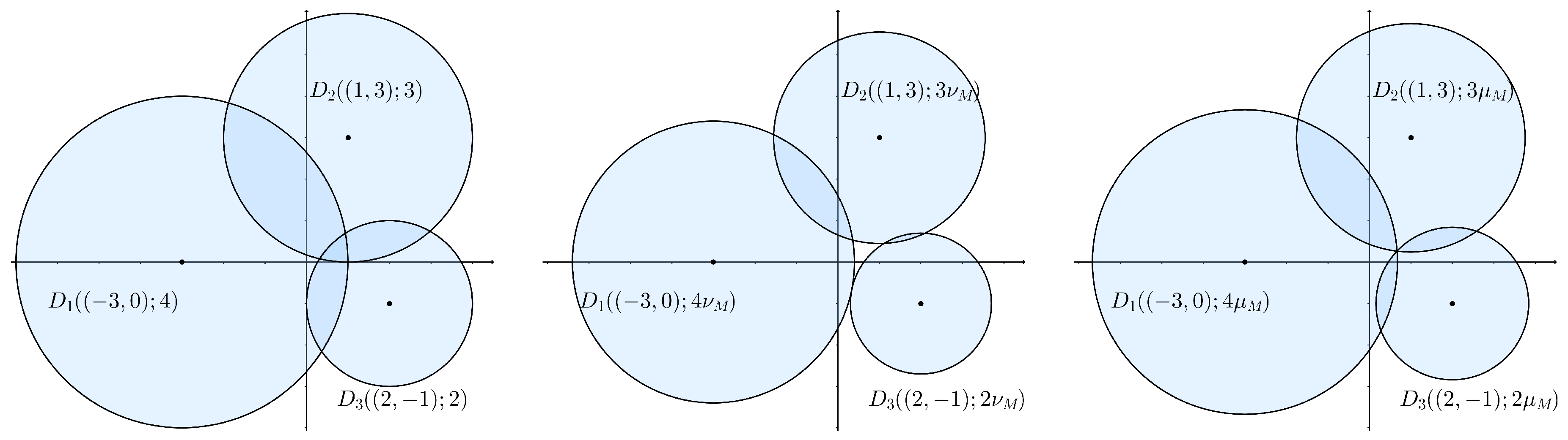
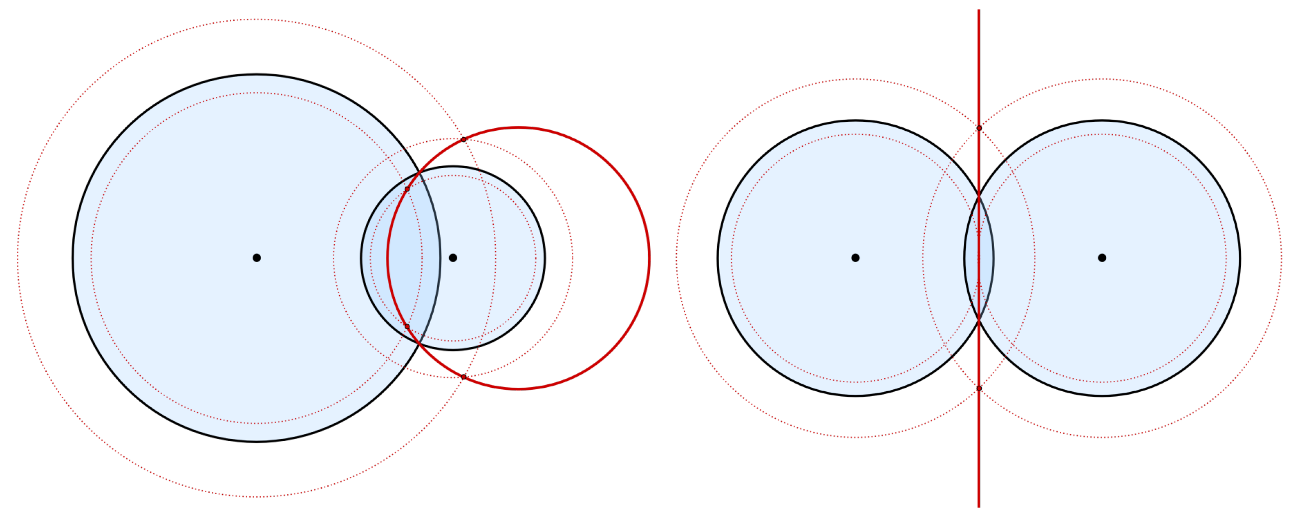
Example 1.

Figure 1 shows (left picture) the following disk system in ${\mathbb{R}}^2$,

$$M=\{D_1((-3,0);4),D_2((1,3);3),D_3((2,-1);2)\}.$$

This 2-disk system is a Vietoris–Rips system and also a Čech system. In this case, we have ${\nu }_M=\sqrt{26}/6\approx 0.8498$, and, in actuality, the ${\nu }_M$-rescaled 2-disk system $M_{{\nu }_M}$ (center picture) has an empty intersection, i.e., ${\bigcap }_{D_i\in M}{D}_i(c_i;{\nu }_M{r}_i)=\varnothing$, so it corresponds to a Vietoris Rips system which is not a Čech system. For such 2-disk system, theCech.scalealgorithm in Section 5 yields to ${\mu }_M=0.9188$ and the Čech system $M_{{\mu }_M}$ is shown in the right picture.

There exists a close relationship between Vietoris–Rips systems and Čech systems. Obviously, every Čech system is also a Vietoris–Rips system, but the opposite statement does not hold in general (as we saw in the example above). However, we have the following result which extends the standard Vietoris–Rips Lemma ([17], Theorem 2.5), to any Vietoris–Rips system; such result can be found in ([18], Theorem 3.2) in the context of weighted simplicial complexes.

The standard Vietoris–Rips Lemma is established in the context of a disk system in which all radii are equal, and corresponds to a reformulation of the well-known Jung’s Lemma [19]. On the other hand, for a disk system in general, the Vietoris–Rips Lemma is also valid, although it does not follow directly from Jung’s Lemma. Next, we propose a proof of the Vietoris–Rips Lemma, for an arbitrary disk system, using elementary geometrical arguments.

Lemma 2.

Let $M=\{D_i(c_i;r_i)\subset {\mathbb{R}}^d\mid r_i>0\}$ be a finite set of closed disks in ${\mathbb{R}}^d$. If $D_i(c_i;r_i)\cap D_j(c_j;r_j)\ne \varnothing$ for every pair of disks in M, then

$$\bigcap _{D_i\in M}{D}_i(c_i;\sqrt{2d/(d+1)}{r}_i)\ne \varnothing .$$

In other words, for every Vietoris–Rips system M in ${\mathbb{R}}^d$, the $\sqrt{2d/(d+1)}$-rescaled disk system $M_{\sqrt{2d/(d+1)}}$ is a Čech system.

Proof. 

First, we prove the result for the case where M has at most $d+1$ disks, say $M=\{D_1,\dots ,D_{d^{\prime }}\}$, $d^{\prime }\le d+1$. Note that we need to prove that ${\mu }_M\le \sqrt{\frac{2d}{d+1}}$.

Let $\left\{c_M\right\}={\bigcap }_i{D}_i(c_i;{\mu }_M{r}_i)$ be the unique intersection point of the ${\mu }_M$-rescaled disk system (see Lemma 1). Without loss of generality, we assume that $\parallel c_i-c_M\parallel ={\mu }_M{r}_i$ for $c_1,\dots ,c_m$ and $m\le d^{\prime }$.

Then, $c_M$ belongs to the convex hull of the set $\{c_1,\dots ,c_m\}$, for if this were not true, there would exist an hyperplane across $c_M$ such that the set $\{c_1,\dots ,c_m\}$ is completely contained at one side, let v be the normal vector for such hyperplane in the opposite direction, then $\langle v,c_i-c_M\rangle >0$ for all $i=1,\dots ,m$, therefore

$$\parallel c_i-c_M{\parallel }^2=\parallel c_i-(c_M+tv){\parallel }^2+2t\langle v,c_i-c_M\rangle -t^2{\parallel v\parallel }^2>{\parallel c_i-(c_M+tv)\parallel }^2$$

for every $t\in I_v:=(0,2\langle v,c_i-c_M\rangle /{\parallel v\parallel }^2)$; this implies that $c_M+tv\in D(c_i;{\mu }_M{r}_i)$ for any $i=1,\dots ,m$ and $t\in I_v$, which is a contradiction since $c_M$ is the only point in the intersection ${\bigcap }_{i}D(c_i;{\mu }_M{r}_i)$. Therefore, $c_M$ is in the convex hull.

Now, define ${\widehat{c}}_i:=c_i-c_M$ and let ${\theta }_{ij}$ denote the angle between vectors ${\widehat{c}}_i$ and ${\widehat{c}}_j$. As $c_M$ is in the convex hull of $\{c_1,\cdots ,c_m\}$, then the vector $0\in {\mathbb{R}}^d$ can be written as a convex combination ${\sum }_{j=1}^m{a}_j{\widehat{c}}_j=0$. Thus, $\langle {\sum }_{j=1}^m{a}_j{\widehat{c}}_j,{\widehat{c}}_i\rangle =0$ for any $i=1,\dots ,m$, and 

$$\sum _{j=1}^m\langle a_j{\widehat{c}}_j,{\widehat{c}}_i\rangle =\sum _{j=1}^m{a}_j\parallel {\widehat{c}}_j\parallel \parallel {\widehat{c}}_i\parallel cos{\theta }_{ji}=0.$$

Taking out the common factor $\parallel {\widehat{c}}_i\parallel$, we have ${\sum }_{j=1}^m{a}_j\parallel {\widehat{c}}_j\parallel cos{\theta }_{ji}=0$. Now, taking the sum over i, we deduce that

$$\sum _{i=1}^m\sum _{j=1}^m{a}_j\parallel {\widehat{c}}_j\parallel cos{\theta }_{ji}=\sum _{j=1}^m{a}_j\parallel {\widehat{c}}_j\parallel \sum _{i=1}^{m}cos{\theta }_{ji}=0.$$

(2)

Note that $cos{\theta }_{ii}=1$. On the other hand, if were $cos{\theta }_{ji}>-{\displaystyle \frac{1}{m-1}}$ for all $1\le i,j\le m$, $i\ne j$, then for each j we should have ${\sum }_{i=1}^{m}cos{\theta }_{ji}=1+{\sum }_{j=1,j\ne i}^{m}cos{\theta }_{ji}>0$. However, this contradicts (2) because ${\sum }_{j=1}^m{a}_j=1$ and $a_j\ge 0$. Therefore, there must exist $i\ne j$, say $i=1$ and $j=2$, such that $cos{\theta }_{12}\le -{\displaystyle \frac{1}{m-1}}\le -{\displaystyle \frac{1}{d}}$, then

$$0\le {\displaystyle \frac{d}{d-1}}(1+cos\left({\theta }_{12}\right))\le 1.$$

(3)

It follows from inequality above and from the AM-GM inequality, that

$$\sqrt{{\displaystyle \frac{d}{d-1}}(1+cos\left({\theta }_{12}\right))}·\sqrt{r_1{r}_2}\le \sqrt{r_1{r}_2}\le {\displaystyle \frac{r_1+r_2}{2}}.$$

(4)

A straightforward calculation on (4) leads us to the following inequality

$$(d+1){(r_1+r_2)}^2\le 2d(r_1^2+r_2^2-2r_1{r}_{2}cos\left({\theta }_{12}\right))$$

so,

$$\begin{array}{cc}\hfill (d+1){\mu }_M^2{(r_1+r_2)}^2& \le 2d({\mu }_M^2{r}_1^2+{\mu }_M^2{r}_2^2-2{\mu }_M^2{r}_1{r}_{2}cos\left({\theta }_{12}\right))\hfill \\ \hfill & =2d(\parallel {\widehat{c}}_1{\parallel }^2+\parallel {\widehat{c}}_2{\parallel }^2-2\parallel {\widehat{c}}_1\parallel \parallel {\widehat{c}}_2\parallel cos\left({\theta }_{12}\right))\hfill \\ \hfill & =2d(\parallel {\widehat{c}}_1{\parallel }^2+\parallel {\widehat{c}}_2{\parallel }^2-2\langle \widehat{c_1},\widehat{c_2}\rangle )=2d\parallel {\widehat{c}}_1-{\widehat{c}}_2{\parallel }^2\hfill \end{array}$$

which implies,

$${\mu }_M^2\le {\displaystyle \frac{2d}{d+1}}·{\displaystyle \frac{\parallel {\widehat{c}}_1-{\widehat{c}}_2{\parallel }^2}{{(r_1+r_2)}^2}}={\displaystyle \frac{2d}{d+1}}·{\displaystyle \frac{\parallel c_1-c_2{\parallel }^2}{{(r_1+r_2)}^2}}\le {\displaystyle \frac{2d}{d+1}}$$

(the last inequality holds because M is a Vietoris–Rips system) or equivalently ${\mu }_M\le \sqrt{\frac{2d}{d+1}}$.

For a collection with more than $d+1$ disks, the claim of the lemma is a consequence of the Helly’s Theorem (see [20], Problem 29), which establishes that for any finite collection, with at least $d+1$ convex subsets of the d-dimensional euclidean space ${\mathbb{R}}^d$, if the intersection of every subcolection with $d+1$ of such sets is nonempty, then the whole collection has a nonempty intersection. This concludes the proof. □

The upper bound $\sqrt{2d/(d+1)}$ in Lemma 2 is optimal: it suffices to take a disk system with $d+1$ disks of equal radii and pairwise tangents (cf. [6], Section III.2).

In the Example 1 we can see what the Vietoris–Rips Lemma claim for the 2-disk system M: ${\mu }_M=0.9188<0.9812=\sqrt{4/3}{\nu }_M$.

To conclude this section, notice that as for a Čech system ${\mu }_M\le 1$, then the Vietoris–Rips Lemma implies the following result.

Corollary 1.

If M is an arbitrary d-disk system and ${\nu }_M$ is its Vietoris–Rips scale, then its Čech scale satisfies that ${\mu }_M\in [{\nu }_M,\sqrt{2d/(d+1)}{\nu }_M]$. In consequence, for every d-disk system M, the rescaled disk system $M_{\sqrt{2d/(d+1)}{\nu }_M}$ is always a Čech system.

In particular, if $\sqrt{2d/(d+1)}{\nu }_M\le 1$ then $M_{{\nu }_M}$ is a Čech system.

3. Filtered Generalized Simplicial Structures for Disk Systems

In this section, we introduce two simplicial structures associated with a disk system M, as well as the filtration induced by rescaling the system M. The importance of these notions lies in their relation to the topological analysis through persistent homology of filtered simplicial structures, induced by point clouds with nonhomogeneous neighborhoods.

Let M be a disk system. Denote by $\mathcal{VR}\left(M\right)$ the family of all Vietoris–Rips subsystems of M, this is,

$$\mathcal{VR}\left(M\right)=\{\sigma \subset M\mid D_i\cap D_j\ne \varnothing ,D_i,D_j\in \sigma \}.$$

Analogously, denote by $\mathcal{C}\left(M\right)$ the set of all Čech subsystems,

$$\mathcal{C}\left(M\right)=\{\sigma \subset M\mid {\cap }_{D_i\in \sigma }{D}_i\ne \varnothing \}.$$

On the other hand, recall that a simplicial structure on a (finite) set V is defined as a family $\Delta \left(V\right)\subset 2^V$ of subsets of V such that if $\sigma \in \Delta \left(V\right)$ and $\tau \subset \sigma$, then $\tau \in \Delta \left(V\right)$. Thus, for any $\sigma \in \mathcal{VR}\left(M\right)$ every disk subsystem $\tau \subset \sigma$ is also in the family $\tau \in \mathcal{VR}\left(M\right)$. The same property is valid for the family $\mathcal{C}\left(M\right)$. These properties imply that $\mathcal{VR}\left(M\right)$ and $\mathcal{C}\left(M\right)$ are simplicial complexes.

We refer to $\mathcal{VR}\left(M\right)$ as the generalized Vietoris–Rips complex associated to the disk system M, and to $\mathcal{C}\left(M\right)$ as the generalized Čech complex of M.

The above construction allows us to perform topological data analysis of point cloud data through the persistent homology of the generalized Vietoris–Rips or Čech complexes. However, to perform such analysis it is necessary to construct a filtered simplicial structure. We will define a filtration through weight functions.

Let $\Delta$ be a simplicial complex and let $\omega :\Delta \to \mathbb{R}$ be a function. We call $\omega$ a weight function over the simplicial complex $\Delta$ if $\tau ,\sigma \in \Delta$ and $\tau \subset \sigma$, implies $\omega \left(\tau \right)\le \omega \left(\sigma \right)$.

For example, to the generalized Čech complex $\mathcal{C}\left(M\right)$ of the disk system M, the function $\omega :\mathcal{C}\left(M\right)\to \mathbb{R},\sigma \mapsto {\mu }_{\sigma }$ which assigns the Čech scale to any Čech subsystem $\sigma \subset M$, is a weight function, called the Čech-weight function. The analogous property holds for the Vietoris–Rips complex and the Vietoris–Rips scale (see [18] for the construction of the filtered generalized Čech complex using weighted point clouds).

Moreover, from the definition we have for the Čech-weight function and to every non-negative scale $\lambda \ge 0$, that

$${\omega }^{-1}\left((-\infty ,\lambda ]\right)=\mathcal{C}\left(M_{\lambda }\right).$$

We denote by ${\mathcal{C}}_M\left(\lambda \right)$ the family $\mathcal{C}\left(M_{\lambda }\right)$ for $\lambda \ge 0$, i.e., the family of all Čech subsystems of the $\lambda$-rescaled disk system $M_{\lambda }$, in order to make the dependence explicit with respect the the parameter. We establish the analogous definition for ${\mathcal{VR}}_M\left(\lambda \right)$, for any $\lambda \ge 0$.

Note that there is no restriction on the scale $\lambda \ge 0$, additional to the non-negativity, i.e., we allow greater values of $\lambda$ than 1, in the interest of studying the generalized Čech complex of rescaled disk systems beyond the original.

For ${\lambda }^{\prime }\le \lambda$ we have the families contention: ${\mathcal{VR}}_M\left({\lambda }^{\prime }\right)\subset {\mathcal{VR}}_M\left(\lambda \right)$ and ${\mathcal{C}}_M\left({\lambda }^{\prime }\right)\subset {\mathcal{C}}_M\left(\lambda \right)$. In general, given a simplicial complex $\Delta$ and a weight function $\omega :\Delta \to \mathbb{R}$, any increasing sequence ${\lambda }_1<\cdots <{\lambda }_s$ of real numbers induces a simplicial filtration: ${\Delta }_1\subset \cdots \subset {\Delta }_s$ for ${\Delta }_i:={\omega }^{-1}\left((-\infty ,{\lambda }_i]\right)$. Thus, for any disk system M, the generalized Čech complex $\mathcal{C}\left(M\right)$ has a filtered simplicial complex structure,

$${\mathcal{C}}_M\left(0\right)\subset \mathcal{C}\left({\lambda }_1\right)\subset \cdots \subset {\mathcal{C}}_M\left({\lambda }_s\right).$$

Of course, when we vary the scale $\lambda$ on a interval the above filtration contains only a finite number of different sets. Moreover, those sets only change when the Čech scale of some disk system is reached, and therefore it is enough to compute all sets corresponding to Čech scales to characterize entirely the filtration. The goal of the next sections is the construction of algorithms to numerically estimate the Čech scale of every Čech subsystem of M.

The filtered generalized Čech complex can be “approximated” by the Vietoris–Rips structure, in the following sense. The inclusion $\mathcal{C}\left(M\right)\subset \mathcal{VR}\left(M\right)$ holds clearly; in consequence, ${\mathcal{C}}_M\left(\lambda \right)\subset {\mathcal{VR}}_M\left(\lambda \right)$ for any scale $\lambda \ge 0$, then by Lemma 2 any Vietoris–Rips d-system $\sigma \in \mathcal{VR}\left(M\right)$ rescaled by a factor of $\sqrt{2d/(d+1)}$ is also a Čech d-system: ${\sigma }_{\sqrt{2d/(d+1)}}\in \mathcal{C}\left(M\right)$. Therefore, for any d-disk system M the following relation is fulfilled:

$${\mathcal{VR}}_M\left({\lambda }^{\prime }\right)\subset {\mathcal{C}}_M\left(\lambda \right)\subset {\mathcal{VR}}_M\left(\lambda \right),$$

where $\sqrt{2d/(d+1)}·{\lambda }^{\prime }\le \lambda$.

To any disk system M, the simplicial substructure $\mathcal{C}{\left(M\right)}^{\left(1\right)}$ given by the 1-skeleton of the generalized Čech complex of M is a basic combinatorial structure (actually, a graph) that can be easily defined, it just takes the relationship into account if every two vertices are neighbors: the set of vertices is M, and there exists an edge $\{D_i,D_j\}$ whenever $D_i\cap D_j\ne \varnothing$. The Čech-weight function restricted to $\mathcal{C}{\left(M\right)}^{\left(1\right)}$ is, in fact: $\omega \left(\left\{D_i\right\}\right)=0$ to every vertice, and $\omega \left(\{D_i,D_j\}\right)=\parallel c_i-c_j\parallel /(r_i+r_j)$ to any edge.

In Algorithm 1, we calculate the Čech-weight function $\omega :{\mathcal{C}}_M{\left(\lambda \right)}^{\left(dim\right)}\to \mathbb{R}$, for the dim-skeleton of a $\lambda$-rescaled disk system M. To do this, we assume an arbitrary linear order in the disk system M, and for every disk $D\in M$ we consider the following set.

$\lambda$-LowerNbrs$\left(D\right)=\{\tilde{D}\in M\mid \tilde{D}<D,\omega \left(\{D,\tilde{D}\}\right)\le \lambda \}$.

The following algorithm (based on work in [7]), is a standard expansion algorithm for simplicial complexes, and we are including the Čech-weight function value of each simplex when it is calculated.

Algorithm 1: Čech-weight function of a d-disk system.

We conclude the section with an application of Algorithm 1 to a 2-disk system.

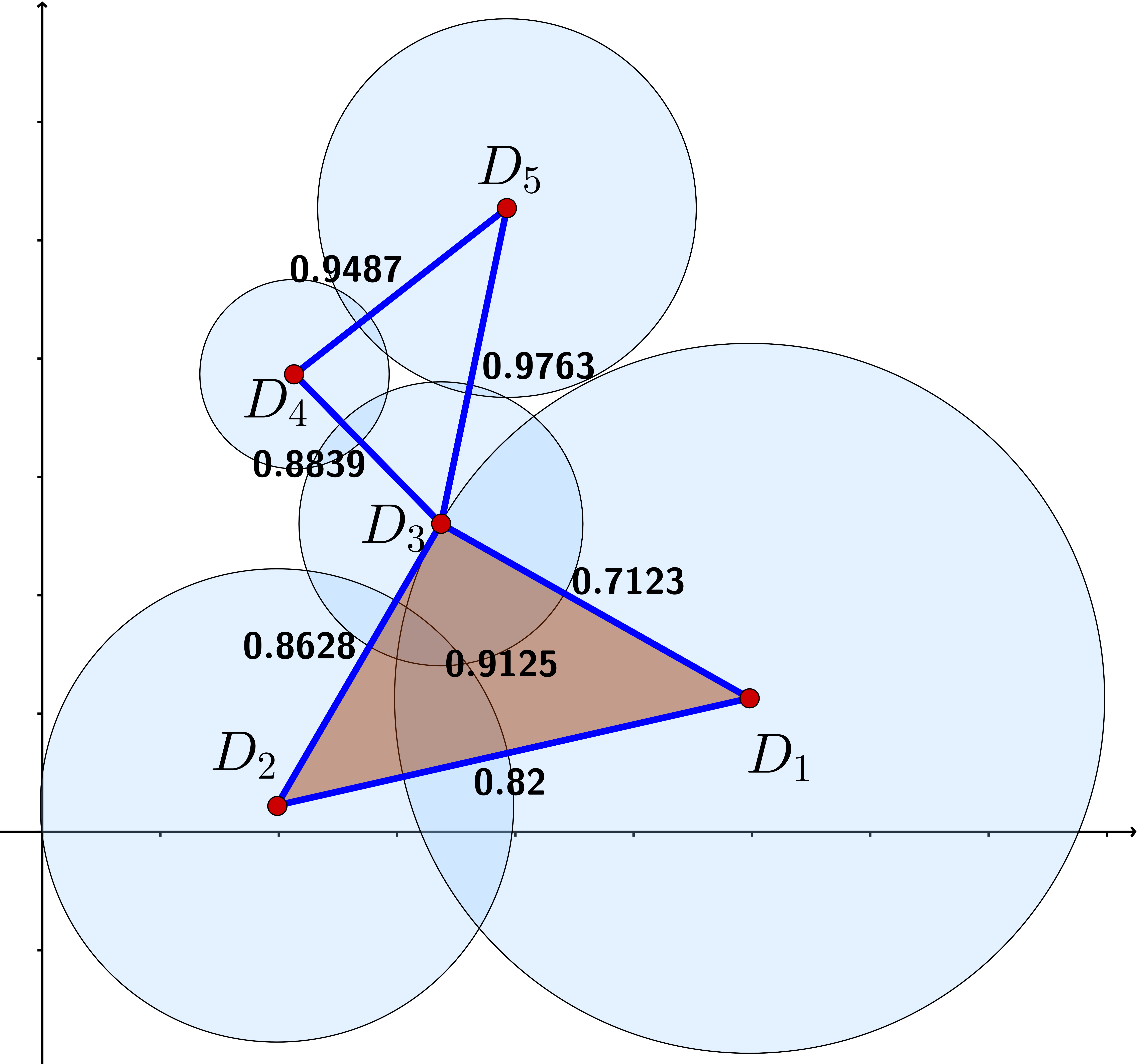
Example 2.

Let M be the following 2-disk system,

$$\begin{array}{cc}\hfill M=\{& D_1((2.99,0.56);1.5),D_2((0.99,0.11);1.0),\hfill \\ \hfill & D_3((1.69,1.30);0.6),D_4((1.07,1.93);0.4),\hfill \\ \hfill & D_5((1.96,2.64);0.8)\}.\hfill \end{array}$$

The output of Algorithm 1 applied to M, with $d=2$, $\lambda =1$ and $dim=2$ gives the Čech scales indicated next to every edge and in the triangle, in Figure 2. The Čech scale of the 2-disk system $\{D_1,D_2,D_3\}$ was calculated with theCech.scalescript from Algorithm 3.   

4. Intersection Properties of Disk Systems

In this section, we focus on studying disk systems in the plane, i.e., 2-disk systems. As we have seen in the last section, the study of the Čech scale is a key aspect to the construction and study of filtered generalized Čech complex. In this section, we establish several intersection properties of 2-disk systems, which will lead us to be able to calculate the Čech scale.

Let $\partial D_i(c_i;r_i):=\{x\in {\mathbb{R}}^2\mid \parallel x-c_i\parallel =r_i\}$ be the boundary of the closed 2-dimensional disk $D_i(c_i,r_i)\subset {\mathbb{R}}^2$.

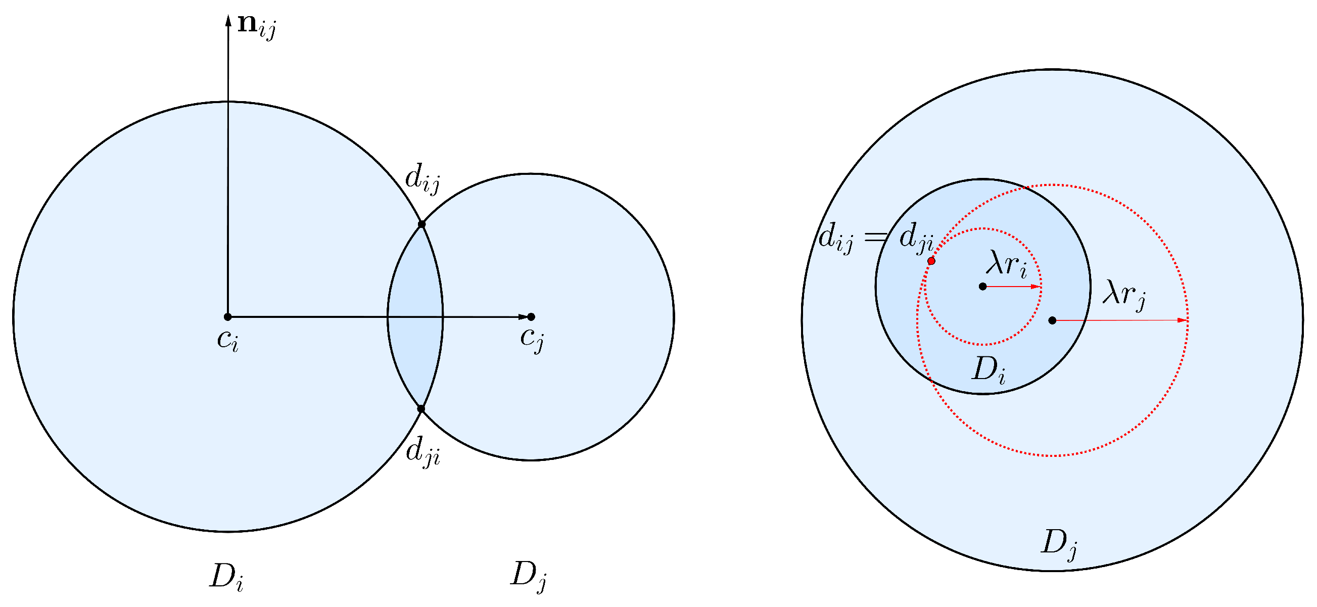
Let $D_i$ and $D_j$ be two closed disks in the plane, such that $D_i\cap D_j\ne \varnothing$. We define $D_i\sqcap D_j$ to be the unitary set $\left\{d_{ij}\right\}$ constructed as follows.

• If $\partial D_i\cap \partial D_j\ne \varnothing$, then $d_{ij}\in \partial D_i\cap \partial D_j$ is the only one point with the property $\langle d_{ij}-c_i,{\mathbf{n}}_{ij}\rangle \ge 0$, where ${\mathbf{n}}_{ij}=(-b,a)$ is the normal vector to $c_j-c_i=(a,b)$,
• If $\partial D_i\cap \partial D_j=\varnothing$, we define $d_{ij}$ as the unique intersection point in $\partial D_i(c_i;\lambda r_i)\cap \partial D_j(c_j;\lambda r_j)$, for $\lambda$ given as the minimal scale such that $D_i(c_i;\lambda r_i)\subset D_j(c_j;\lambda r_j)$ or $D_j(c_j;\lambda r_j)\subset D_i(c_i;\lambda r_i)$, i.e., $\lambda =\parallel c_i-c_j\parallel /|r_i-r_j|$.

Clearly, if $\partial D_i\cap \partial D_j=\varnothing$, then $d_{ij}=d_{ji}$. In particular, when $D_i$ and $D_j$ are concentric, then $D_i\sqcap D_j=\left\{c_i\right\}=\left\{c_j\right\}$. On the other hand, if the closed disks $D_i$ and $D_j$ are internally or externally tangent, then $d_{ij}=d_{ji}$. We can think about $d_{ij}$, when $\partial D_i\cap \partial D_j$ is not empty, as the intersection point of the boundaries at the left of the vector from $c_i$ to $c_j$. Figure 3 shows the above construction.

We will denote by $d_{ij}\left(\lambda \right)$, instead of simply $d_{ij}$, for the intersection point of the $\lambda$-rescaled disks $D_i(c_i;\lambda r_i)$ and $D_j(c_j;\lambda r_j)$.

In order to study Čech systems, we give the following characterization, according the intersection points $d_{ij}$.

Lemma 3.

Let $M=\{D_1,D_2,\dots ,D_m\}$ be a 2-disk system. Then M is a Čech system if and only if, there exist $D_i,D_j\in M$ such that $d_{ij}\in D_i\sqcap D_j$ satisfies $d_{ij}\in D_k$ for all $1\le k\le m$.

Proof. 

Suppose M is a Čech system. Define $A:={\bigcap }_{1\le i\le m}{D}_i\ne \varnothing$; then, A has only one of the following geometries.

(i)

$A=\left\{c_M\right\}$,

(ii)

A is a region bounded by more than one circumference arc,

(iii)

$A=D_{i_0}$ for some $i_0\in \{1,\dots ,m\}$.

In the first case, necessarily $c_M$ belongs to the boundary of two or more disks. Let $D_i$ and $D_j$ be two disks in M such that $c_M\in \partial D_i\cap \partial D_j$, it follows that $c_M=d_{ij}$ or $c_M=d_{ji}$, in both cases the lemma holds.

For the second case, if $a\in \partial A\subset A$ belongs to the boundary and is in the intersection of two arcs, say $\partial D_i$ and $\partial D_j$, then $a=d_{ij}$ or $a=d_{ji}$, and it satisfy $a\in D_k$ for every $1\le k\le m$.

For the last case, if $A=D_{i_0}$ for some $i_0$, then for each $j\ne i_0$ we have $d_{i_{0}j}\in D_{i_0}=A$ and all of these points belongs to $D_k$ for all $D_k\in M$.

Therefore, in any case, there exists such point $d_{ij}$. The converse is clear by definition of a Čech system. □

This criterion was presented in ([8], Section III) for a 2-disk system.

Next, we define the map $\rho$, a key tool for the rest of this work. This map will allow us to discern the minimal scale in which a 2-disk system has the nonempty intersection property.

Definition 3.

Let $M=\{D_1,D_2,\dots ,D_m\}$ be a Vietoris–Rips system in the plane, with $m\ge 3$. We define

$$\rho \left(M\right):=\underset{1\le i,j\le m}{max}\left\{\underset{k\ne i,j}{min}\{r_k-\parallel d_{ij}-c_k\parallel \}\right\}.$$

If ${\nu }_M$ is the Vietoris–Rips scale of M, then we define the map ${\rho }_M:[{\nu }_M,\infty )\to \mathbb{R}$, $\lambda \mapsto {\rho }_M\left(\lambda \right)=\rho \left(M_{\lambda }\right)$.

Given three disks $D_i(c_i;r_i)$, $D_j(c_j;r_j)$ and $D_k(c_k;r_k)$ in the 2-disk system $M=\{D_1,\dots ,D_m\}$, with Vietoris–Rips scale ${\nu }_M$, denote by ${\mathsf{\Lambda }}_{i,j}^k:[{\nu }_M,\infty )\to \mathbb{R}$ the map $\lambda \mapsto \lambda r_k-\parallel d_{ij}\left(\lambda \right)-c_k\parallel$, where $d_{ij}\left(\lambda \right)$ is the element in $D_i(c_i;\lambda r_i)\sqcap D_j(c_j;\lambda r_j)$. In other words, ${\mathsf{\Lambda }}_{i,j}^k\left(\lambda \right)$ is the signed distance from the point $d_{ij}\left(\lambda \right)$ to the set $D_k(c_k;\lambda r_k)$.

If $r_i\ne r_j$, then for each $k\ne i,j$ the map $\lambda \mapsto \lambda r_k-\parallel d_{ij}\left(\lambda \right)-c_k\parallel$ is defined and continuous in the closed interval $\left[\parallel c_i-c_j\parallel /(r_i+r_j),\parallel c_i-c_j\parallel /|r_i-r_j|\right]$, as it is the signed distance from an intersection point of two continuously deforming curves (therefore its position vary continuously as long as the intersection exists) to the continuously deforming set $D_k(c_k;\lambda r_k)$ with respect to $\lambda$. Also, the map $\lambda \mapsto \lambda r_k-\parallel d_{ij}\left(\lambda \right)-c_k\parallel$ vary linearly in the range $[\parallel c_i-c_j\parallel /|r_i-r_j|,\infty )$ because for $\lambda \ge \parallel c_i-c_j\parallel /|r_i-r_j|$, the term $\parallel d_{ij}\left(\lambda \right)-c_k\parallel$ remains constant. The left picture in Figure 4 shows in bold red color the geometric place of $\{d_{ij}\left(\lambda \right),d_{ji}\left(\lambda \right)\}$, which vary continuously respect to the parameter $\lambda$ and also the distance from it to the fix point $c_k$.

On the other hand, for $r_i=r_j$, the points $\{d_{ij}\left(\lambda \right),d_{ji}\left(\lambda \right)\}$ vary continuously respect to $\lambda$ on the line showed in the right picture of Figure 4. Therefore, $\lambda r_k-\parallel d_{ij}\left(\lambda \right)-c_k\parallel$ also depend continuously of $\lambda$.

From the above argument, each map ${\mathsf{\Lambda }}_{i,j}^k$ is continuous in the interval $[{\nu }_M,\infty )$, and by the continuity of the min-max functions and that

$${\rho }_M\left(\lambda \right)=\underset{1\le i,j\le m}{max}\left\{\underset{k\ne i,j}{min}{\mathsf{\Lambda }}_{i,j}^k\left(\lambda \right)\right\},$$

it follows that ${\rho }_M$ is also a continuous map in the interval $[{\nu }_M,\infty )$. However, the map ${\rho }_M$ is not differentiable, in general, to every point in such interval.

The map ${\rho }_M$ plays a key role in the rest of this work. We present the next characterization of Čech systems in terms of ${\rho }_M$.

Lemma 4.

Let M be a 2-disk system. Then $M_{\lambda }$ is a Čech system if and only if, ${\rho }_M\left(\lambda \right)\ge 0$. In particular ${\rho }_M\left(\sqrt{4/3}{\nu }_M\right)\ge 0$.

Proof. 

By Lemma 3, $M_{\lambda }$ is a Čech system in the plane if and only if, there exists $d_{ij}\left(\lambda \right)$ such that $d_{ij}\left(\lambda \right)\in D_k(c_k;\lambda r_k)$ for every $k\ne i,j$, i.e., ${\mathsf{\Lambda }}_{i,j}^k\left(\lambda \right)\ge 0$ for every $k\ne i,j$, which is equivalent to ${\rho }_M\left(\lambda \right)\ge 0$.

On the other hand, from Corollary 1 and taking $d=2$, the rescaled system $M_{\sqrt{4/3}{\nu }_M}$ is a Čech system, then by the first assertion, ${\rho }_M\left(\sqrt{4/3}{\nu }_M\right)\ge 0$. □

5. The Cech.scale Algorithm

Our main algorithm (Algorithm 3) computes the Čech scale of a given 2-disk system M. The key aspect on which this algorithm is based, is precisely the function ${\rho }_M$. Before we describe the algorithm, we need to analyze additional properties of ${\rho }_M$.

It follows immediately from Lemma 4 that ${\rho }_M\left(\lambda \right)\ge 0$ for every $\lambda \ge {\mu }_M$. Also, if at the Vietoris–Rips scale it holds that ${\rho }_M\left({\nu }_M\right)\ge 0$, then ${\mu }_M={\nu }_M$ by the minimality of the Čech scale. We conclude that in this case (this is, ${\rho }_M\left({\nu }_M\right)\ge 0$), the Čech scale is easily computable.

On the other hand, if ${\rho }_M\left({\nu }_M\right)<0$ then the Čech scale satisfies ${\mu }_M\in ({\nu }_M,\sqrt{4/3}{\nu }_M]$ and moreover ${\rho }_M\left({\mu }_M\right)=0$. This is a consequence of the continuity of ${\rho }_M$, and the fact that ${\rho }_M\left(\lambda \right)<0$ for every ${\nu }_M\le \lambda <{\mu }_M$ and ${\rho }_M\left(\lambda \right)\ge 0$ for ${\mu }_M\le \lambda$. Thus, to find the Čech scale of a 2-disk system M for which ${\rho }_M\left({\nu }_M\right)<0$, we need to solve the equation ${\rho }_M\left(\lambda \right)=0$.

We propose a numerical approach to solve the equation ${\rho }_M\left(\lambda \right)=0$ and calculate the Čech scale under the hypothesis ${\rho }_M\left({\nu }_M\right)<0$, as in this case, we actually know that ${\mu }_M\in ({\nu }_M,\sqrt{4/3}{\nu }_M]$ (see Section 2) as consequence of the generalized Vietoris–Rips Lemma. We chose the bisection method for this purpose. We will denote the implementation of bisection method for the map ${\rho }_M$ through the interval $[a,b]$, by bisection $({\rho }_M,a,b)$. The output of bisection $({\rho }_M,a,b)$ is a real number $\lambda \in [a,b]$ such that ${\rho }_M\left(\lambda \right)=0$. For the numerical method we are working with a precision of ${10}^{-12}$.

It is important to mention that the numerical method regula falsi was also used instead of the numerical method of bisection, in order to calculating the Čech scale. However, in our context, the efficiency of the program using the regula falsi numerical method is not better than if the numerical method of bisection is used.

The Algorithm 2 (below) has as input a 2-disk system M, and produces as output the Čech scale ${\mu }_M$ as well as the intersection point $\left\{c_M\right\}={\bigcap }_{D_i\in M}{D}_i(c_i;{\mu }_M{r}_i)$. This algorithm takes a naive approach to calculate the Čech scale, and is established to completeness and to be a reference for the principal algorithm (Algorithm 3).   

Algorithm 2: The Čech scale calculation for a 2-disk system.

The following lemma claims that the Algorithm 2 is consistent.

Lemma 5.

For any 2-disk system M, the Algorithm 2 has as output the Čech scale ${\mu }_M$ of M, and the unique intersection point $\left\{c_M\right\}={\bigcap }_{D_i\in M}{D}_i(c_i;{\mu }_M{r}_i)$.

Proof. 

In the case ${\rho }_M\left({\nu }_M\right)\ge 0$, it is clear that the algorithm has generated asseverated data (steps (2)–(3)). In otherwise, for the case ${\rho }_M\left({\nu }_M\right)<0$, we assign ${\mu }^{*}:=\sqrt{4/3}{\nu }_M$.

Then, ${\rho }_M\left({\nu }_M\right)·{\rho }_M\left({\mu }^{*}\right)\le 0$ and lets call again ${\mu }^{*}$ the output root in step (7). To check if ${\mu }^{*}$ is the Čech scale we are looking for, we calculate in step (8) the set of pairwise intersection points of the ${\mu }^{*}$-rescaled system, contents in ${\bigcap }_{D_i\in M}{D}_i(c_i;{\mu }^{*}{r}_i)$.

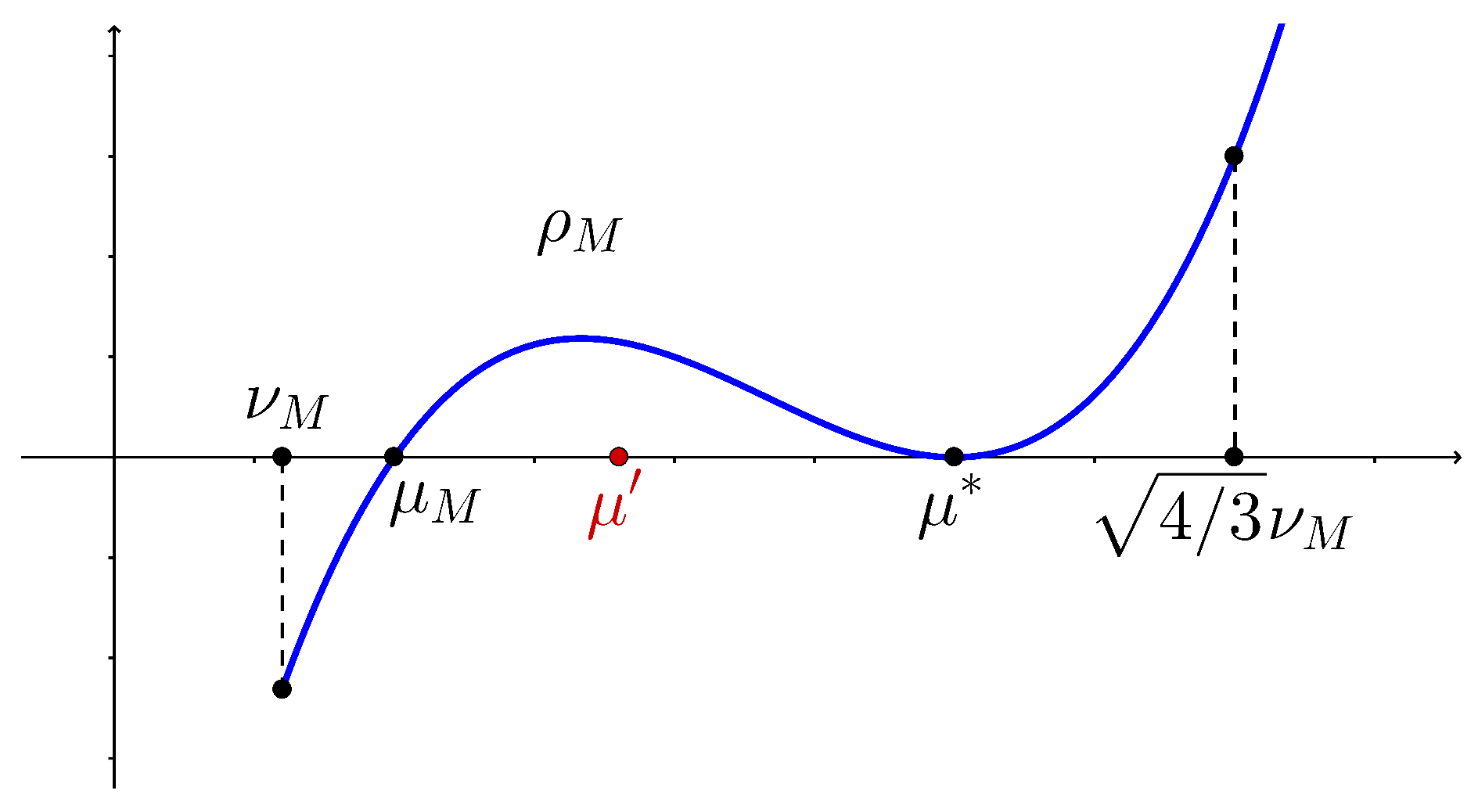
If the set $\sqcap M_{{\mu }^{*}}$ is unitary, then necessarily ${\bigcap }_{D_i\in M}{D}_i(c_i;{\mu }^{*}{r}_i)$ is unitary, due the geometry of its boundary (see proof of Lemma 3). In such case (negative validation of step (9)) the steps (10)–(13) are omitted and, from Lemma 1, the algorithm returns the Čech scale as well as the intersection point $\sqcap M_{{\mu }^{*}}$ at step (14); in otherwise (positive validation of step (9)), the root ${\mu }^{*}$ is not the Čech scale (see Figure 5), and then we should find another scale ${\mu }^{\prime }\in ({\nu }_M,{\mu }^{*})$ such that ${\rho }_M\left({\mu }^{\prime }\right)>0$, and repeat from step (7). It is possible, for some configurations of the 2-disk system, that the map ${\rho }_M$ has a behavior as in Figure 5.

The last iterative part is a finite process because ${\rho }_M$ is algebraic over $\mathbb{Q}$, then eventually the set $\sqcap M_{{\mu }^{*}}$ will be unitary and the Čech scale will be calculated. □

The step (8) in Algorithm 2 is necessary, as show the following example, in which the map ${\rho }_M$ has another root along side the Čech scale in the interval $[{\nu }_M,\sqrt{4/3}{\nu }_M]$.

Example 3.

Let $M=\{D_1,D_2,D_3\}$ be the 2-disk system in Figure 6. A direct calculation, yields that ${\nu }_M={\mu }_M=0.8947$. On the other hand, we also have that ${\rho }_M\left({\nu }_M\right)={\rho }_M\left({\mu }_M\right)={\rho }_M\left(\lambda \right)=0$ for $\lambda =1$. Therefore, the map ${\rho }_M$ has more than one root on the interval $[{\nu }_M,\sqrt{4/3}{\nu }_M]=[0.8947,1.0331]$.

In Example 3, the Vietoris–Rips scale ${\nu }_M$, of the 2-disk system M, agrees with the Čech scale ${\mu }_M$; however is possible to construct more sophisticated (and symmetric) disk system M such that ${\nu }_M<{\mu }_M$ and ${\rho }_M\left({\nu }_M\right)<0<{\rho }_M\left({\mu }_M\right)$, for which there exists ${\mu }^{\prime }\in (\nu ,\sqrt{4/3}{\nu }_M)$ with ${\rho }_M\left({\mu }^{\prime }\right)=0$.

On the other hand, if the 2-disk system M consists of just three disks and ${\rho }_M\left({\nu }_M\right)<0$, then its Čech scale can be computed with only one application of the numerical method, as we asseverate in the following lemma.

Lemma 6.

Let $M=\{D_1,D_2,D_3\}$ be a 2-disk system such that ${\rho }_M\left({\nu }_M\right)<0$. Then, there exists a unique root of the map ${\rho }_M$ in $[{\nu }_M,\sqrt{4/3}{\nu }_M]$. Thus, ${\mu }_M$ will be the output ofbisection$({\rho }_M,{\nu }_M,\sqrt{4/3}{\nu }_M)$.

Proof. 

It is straightforward to verify that ${\rho }_M\left({\nu }_M\right)\ge 0$ for any configuration with $c_1$, $c_2$ and $c_3$ collinear. Thus, it follows $\{c_1,c_2,c_3\}$ is in general position.

Let ${\mu }_M$ be the Čech scale of the 2-disk system M and $c_M$ the intersection point. Define $A\left(\lambda \right):={\cap }_{i=1}^3{D}_i(c_i;\lambda r_i)$. Note that $A\left({\mu }_M\right)=\left\{c_M\right\}$.

We claim that there exist at least two distinct points p and q, in the set

$$\{d_{ij}\left(\lambda \right)\in D_i(c_i;\lambda r_i)\sqcap D_j(c_j;\lambda r_j)\mid D_i,D_j\in M_{\lambda }\}\subset \partial A\left(\lambda \right).$$

This is evident if $\partial A\left(\lambda \right)$ is given by two or more circumference arcs. On the other hand, if $\partial A\left(\lambda \right)=\partial D_i(c_i;\lambda r_i)$ for some $1\le i\le 3$, then $d_{ij}\left(\lambda \right),d_{ik}\left(\lambda \right)\in D_i(c_i;\lambda r_i)$ for $j\ne i$ and $k\ne i$. Moreover, $d_{ij}\left(\lambda \right)\ne d_{ik}\left(\lambda \right)$ since $\{c_1,c_2,c_3\}$ is not a collinear set.

If both points p and q belongs to each boundary of the three disks, $p,q\in {\cap }_{i=1}^3\partial D_i(c_i;\lambda r_i)$, then $\{c_1,c_2,c_3\}$ would be also a collinear set. Without loss of generality, we suppose that $p=d_{23}\left(\lambda \right)\notin \partial D_1(c_1;\lambda r_1)$. Then, ${\rho }_M\left(\lambda \right)\ge \lambda r_1-\parallel d_{23}\left(\lambda \right)-c_1\parallel >0$, and the lemma follows. Of course, the choose of the indexes depend of the value of $\lambda$, but the above arguments show that always there exist such combination which guarantee that ${\rho }_M\left(\lambda \right)$ is positive for $\lambda >{\mu }_M$. □

The following algorithm takes advantage of the unicity property for the root of ${\rho }_M$, in a 2-disk system with three disks. Essentially, the algorithm consist in iterating the Algorithm 2 systematically over every triplet of disks from M.   

Algorithm 3:Cech.scale.

Theorem 1.

For any 2-disk system M, the Algorithm 3 has as output the Čech scale ${\mu }_M$ of M, and the unique intersection point $\left\{c_M\right\}={\bigcap }_{D_i\in M}{D}_i(c_i;{\mu }_M{r}_i)$.

Proof. 

If ${\rho }_M\left({\nu }_M\right)\ge 0$, the algorithm returns the right data: steps (1)–(5).

On the other hand, by Helly’s Theorem (cf. [20]) the 2-disk system $M=\{D_1,\dots ,D_m\}$, as a finite family of convex sets in the plane, has a nonempty intersection ${\bigcap }_{D_i\in M}{D}_i$ if, and only if, $D_i\cap D_j\cap D_k\ne \varnothing$ for every triplet $1\le i<j<k\le m$. Let $\mu$ be the maximal Čech scale over every triplet in the disk system M, i.e., 

$$\mu =max\{{\mu }_N\mid N=\{D_i,D_j,D_k\}\subset M\}.$$

It follows that every $\mu$-rescaled triplet has a nonempty intersection. Therefore, the $\mu$-rescaled 2-disk system $M_{\mu }$ also has the nonempty intersection property. Moreover, ${\bigcap }_{D_i\in M}{D}_i(c_i;\mu r_i)\subset {\bigcap }_{D_i\in N\subset M}{D}_i(c_i;\mu r_i)$ for every triplet $N\subset M$. Therefore, $\mu$ is actually the Čech scale of the 2-disk system M, this is, ${\mu }_M=\mu$.

In steps (6)–(19), the algorithm search the scale $\mu$ systematically, over every triplet $\{D_i,D_j,D_k\}\subset M$, updating the maximal scale found if necessary in steps (15)–(17). By Lemma 6, every Čech scale calculation over any triplet, requires just one application of the bisection method. This implies the correctness of the algorithm.

Additionally, the condition in step (9) avoids calculating unnecessary Čech scales of triplets $N=\{D_i,D_j,D_k\}$. In effect, if ${\lambda }^{*}$ is the maximal Čech scale found until the verification of the triplet N, and the condition in step (9) does not satisfy, i.e.,

$${\mu }_N\le \sqrt{4/3}{\nu }_M<{\lambda }^{*},$$

then, whatever is the Čech scale of N, it would be not greater than ${\lambda }^{*}$. □

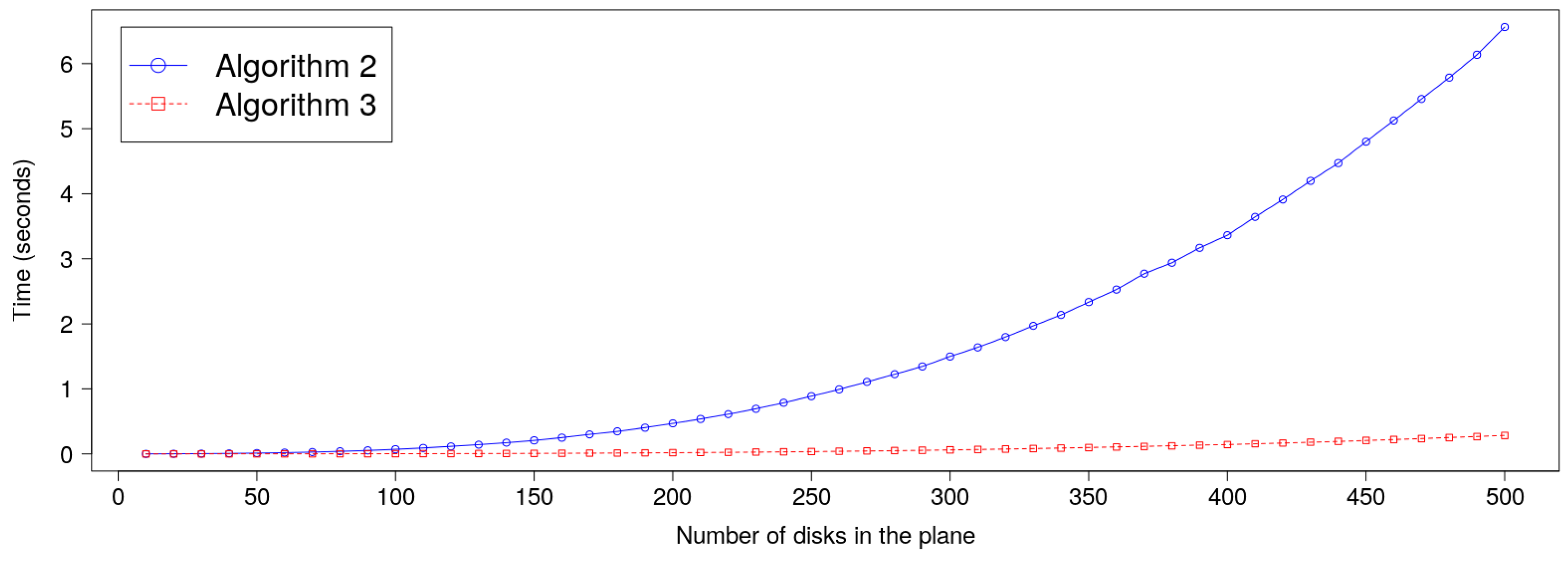
The computational evidence to support the Algorithm 3 is more efficient than Algorithm 2, is given in Figure 7. The graphic shows the average time (in seconds) to computation of both algorithms, with respect to the number of disks in a randomly generated 2-disk system (see Remark 1).

An Example: The Miniball Problem

The miniball problem or smallest-circle problem in the euclidean space is a classical problem, proposed by James J. Sylvester in 1857.

Given a finite point cloud $N\subset {\mathbb{R}}^d$, the miniball problem consists in finding the center $c\in {\mathbb{R}}^d$ and minimum radius $r\in {\mathbb{R}}^{+}$ of a d-disk $D=D(c;r)\subset {\mathbb{R}}^d$ such that $N\subset D$.

There exist many different approaches to solve this problem, and a variety of algorithms to reach the miniball data (e.g., [21,22]). In fact, the Čech scale has a close relation with the miniball problem, as we establish in the next lemma.

Lemma 7.

Let N be a finite point cloud in ${\mathbb{R}}^d$, and let $N_1$ be the associated d-disk system defined by

$$N_1:=\{D_i(c_i;1)\subset {\mathbb{R}}^d\mid c_i\in N\}.$$

Then, the Čech scale ${\mu }_{N_1}$ is the radius of the minimal enclosing ball of N, and the intersection point $\left\{c_{N_1}\right\}={\bigcap }_{c_i\in N}{D}_i(c_i;{\mu }_{N_1})$ its center.

Proof. 

Let ${\mu }_{N_1}$ be the Čech scale of the disk system $N_1$, and let $c_{N_1}$ be the intersection point of the ${\mu }_M$-rescaled disk system. Then, the point $c_{N_1}$ belongs to every disk $D_i(c_i;{\mu }_{N_1}·1)$, i.e., $\parallel c_i-c_{N_1}\parallel \le {\mu }_{N_1}$ for any $c_i\in N$; thus, $N\subset D(c_{N_1};{\mu }_{N_1})$. On the other hand, by definition of Čech scale, ${\mu }_{N_1}$ is the minimal radius (scale) with such property. Therefore, by uniqueness, $D(c_{N_1};{\mu }_{N_1})$ must be the minimal ball enclosing the point cloud N. □

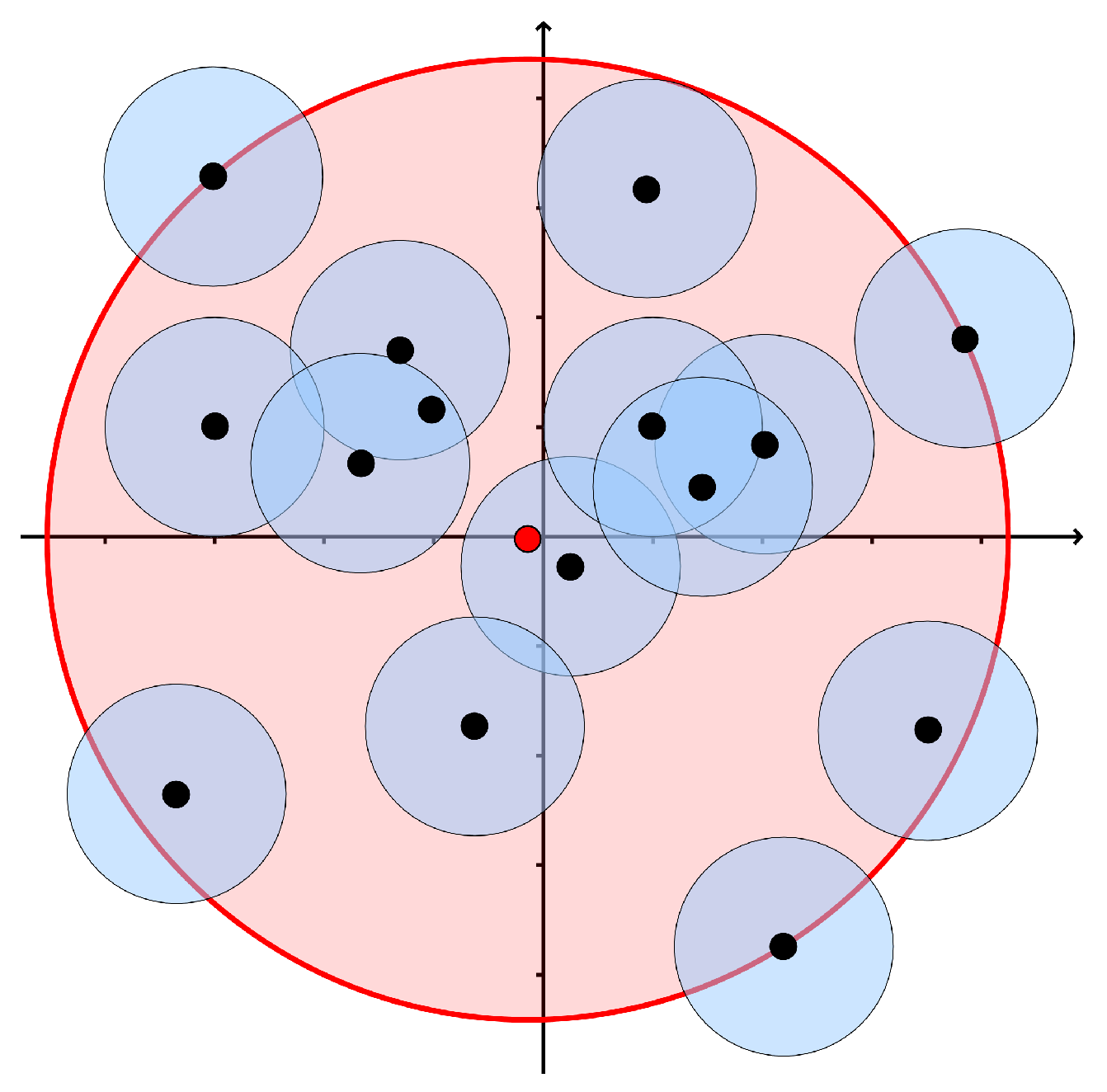
In particular, for a point cloud N in the plane we can apply our algorithm Cech.scale (Algorithm 3) to the 2-disk system $N_1$, and get the minimal enclosing ball of N. However, the Čech scale of an arbitrary 2-disk system $M=\{D_1(c_1;r_1),\dots ,D_m(c_m;r_m)\}$ cannot be obtained from the minimal enclosing ball data of the point cloud $M_0=\{c_1,\dots ,c_m\}$.

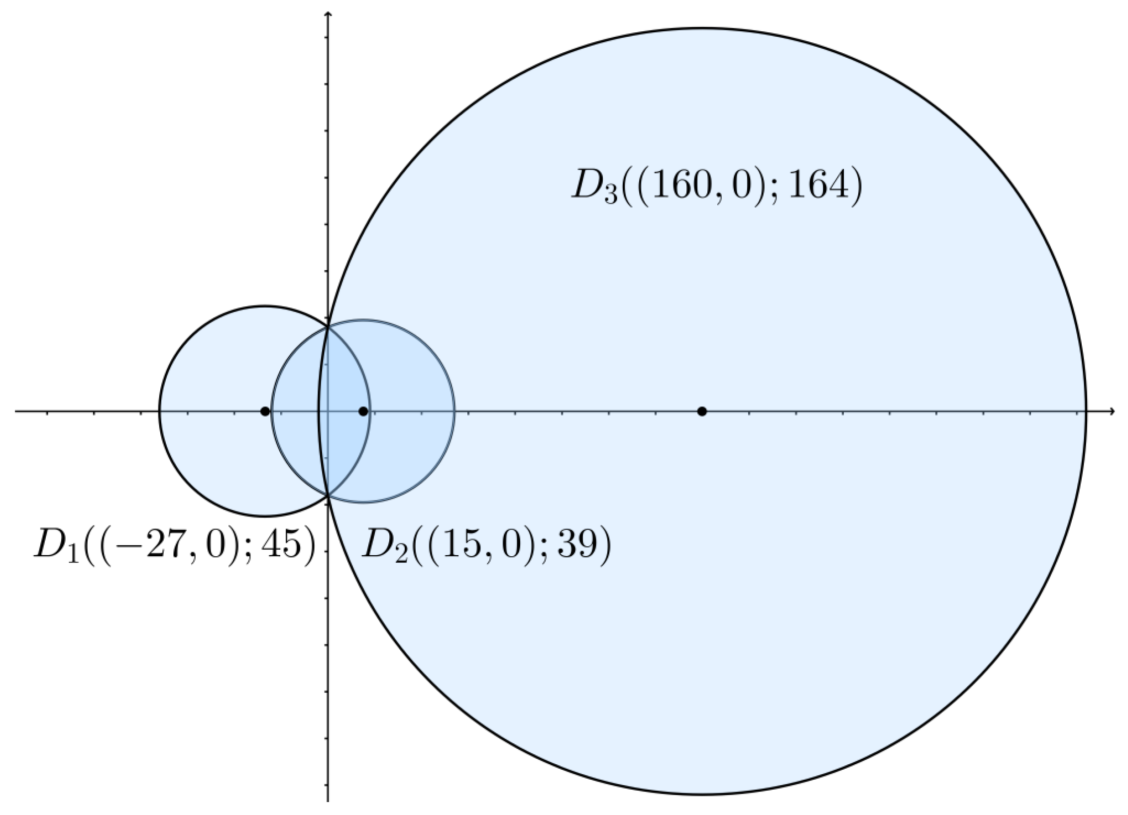
In Figure 8, we show a point cloud N (black dots) and the 2-disk system $N_1$ (blue circles). Applying the Cech.scale script to $N_1$ we get the Čech scale ${\mu }_{N_1}$ (radio of the red circle) and the point $c_{N_1}$ (red point, center of the red circle).

For the miniball problem there are many efficient algorithms available online, which are easy to find. For example, the C++ script in [23] can compute the miniball for point clouds in any dimension (efficiently up to dimension 10,000). Such algorithms are not comparable with the Cech.scale algorithm because if only disk systems with equal (and unitary) radii were considered, several issues that were addressed in the case of different radii would be avoided.

6. The Algorithm Cech.scale for Higher-Dimensional Disk Systems

It is not clear how to generalize the Algorithm 3 to determine the Čech scale of a disk system in ${\mathbb{R}}^d$ with $d>2$. However, it is possible to calculate the Čech scale if the d-disk system consists of only three disks. This makes it possible to calculate the 2-skeleton associated with a d-disk system in an arbitrary dimension.

The relevance of this application lies in the possibility of calculating the 2-dimensional filtered simplicial Čech structure of a disk system immersed in a high-dimensional euclidean space. Many applications in topological data analysis concerns to the study of low-dimensional topological features associated to a point data cloud immersed in a high-dimensional representation space.

The key observation is that

$$\bigcap _{i=1}^{3}D(c_i;r_i)\ne \varnothing \iff \bigcap _{i=1}^3(D(c_i;r_i)\cap P)\ne \varnothing ,$$

where P is the affine plane generated by the set $\{c_1,c_2,c_3\}$.

Thus, the problem of determining whether ${\displaystyle \bigcap _{i=1}^3(D(c_i;r_i)\cap P)}$ is empty or not, can be treated as one in the plane, constructing a disk system in ${\mathbb{R}}^2$ that preserves the affine configuration of the points $\{c_1,c_2,c_3\}$ in the affine space $P\subset {\mathbb{R}}^d$. To do this, we set the first center $c_1$ as the origin in ${\mathbb{R}}^2$, and “translate” the others centers preserving their original configuration, taking care of moving the second center on the x-axis, as in Figure 9.

More precisely, to any d-disk system with three elements, say $M=\{D_1(c_1;r_1),D_2(c_2;r_2),D_3(c_3;r_3)\}$, we associate the following 2-disk system, which clearly preserves the affine configuration of the original centers $\{c_1,c_2,c_3\}$,

$$\mathrm{Aff}\left(M\right)=\{D_1({\tilde{c}}_1;r_1),D_2({\tilde{c}}_2;r_2),D_3({\tilde{c}}_3;r_3)\}$$

where ${\tilde{c}}_1:=(0,0)$, ${\tilde{c}}_2:=(\parallel c_2-c_1\parallel ,0)$, ${\tilde{c}}_3:=(\parallel c_3-c_1\parallel cos\left(\theta \right),\parallel c_3-c_1\parallel sin\left(\theta \right))$, where $\theta$ is the angle between the vectors $c_2-c_1$ and $c_3-c_1$, which satisfies the following relationship:

$$cos\theta ={\displaystyle \frac{\langle c_2-c_1,c_3-c_1\rangle }{\parallel c_2-c_1\parallel ·\parallel c_3-c_1\parallel }}.$$

The Algorithm 4 is a variant of Algorithm 1, taking as input a d-disk system in ${\mathbb{R}}^d$ and a non-negative parameter $\lambda$, and as output the Čech weight function of the 2-skeleton of the generalized Čech complex structure. The algorithm first preprocess each triplet of d-disks as a 2-disk system, then the Čech scale is calculated.  

Algorithm 4: 2-skeletal Čech-weight function.

Figure 10 shows the performance (in ${10}^{-6}$ s) of the C/C++ script Cech.scale (available in [24]) and the preprocessing of the d-disk system to a 2-disk system.

Remark 1.

All our timings were done on a 64-bit GNU/Linux machine with two Intel Xeon processors (3.40 GHz), although our script were not threaded and only one core was used per process. We measured all the timings withclock()from the Standard C library. The average times in both graphics (Figure 7 and Figure 10) are the mean times for ${10}^4$ repetitions of each algorithm, for every number of disks multiple of 10 in Figure 7 from 10 to 500, and for every dimension multiple of 200 in Figure 10 from 200 to 10,000.

References

- Carlsson, G. Topology and data. Bull. Am. Math. Soc. 2009, 46, 255–308. [Google Scholar] [CrossRef] [Green Version]
- Carlsson, G. Topological pattern recognition for point cloud data. Acta Numer. 2014, 23, 289–368. [Google Scholar] [CrossRef] [Green Version]
- Ghrist, R. Barcodes: The persistent topology of data. Bull. Am. Math. Soc. 2008, 45, 61–75. [Google Scholar] [CrossRef] [Green Version]
- Lum, P.Y.; Singh, G.; Lehman, A.; Ishkanov, T.; Vejdemo-Johansson, M.; Alagappan, M.; Carlsson, J.; Carlsson, G. Extracting insights from the shape of complex data using topology. Sci. Rep. 2013, 3. [Google Scholar] [CrossRef] [PubMed] [Green Version]
- Zomorodian, A.; Carlsson, G. Computing persistent homology. Discret. Comput. Geom. 2005, 33, 249–274. [Google Scholar] [CrossRef] [Green Version]
- Edelsbrunner, H.; Harer, J. Computational Topology: An Introduction; American Mathematical Society: Providence, RI, USA, 2010. [Google Scholar]
- Zomorodian, A. Fast construction of the Vietoris-Rips complex. Comput. Graph. 2010, 34, 263–271. [Google Scholar] [CrossRef]
- Le, N.K.; Martins, P.; Decreusefond, L.; Vergne, A. Construction of the Generalized Čech Complex. In Proceedings of the 2015 IEEE 81st Vehicular Technology Conference (VTC Spring), Glasgow, UK, 11–14 May 2015; pp. 1–5. [Google Scholar] [CrossRef]
- Dantchev, S.; Ivrissimtzis, I. Efficient construction of the Čech complex. Comput. Graph. 2012, 36, 708–713. [Google Scholar] [CrossRef]
- Morozov, D. Dionysus 2. 2019. Available online: http://mrzv.org/software/dionysus2/ (accessed on 23 October 2019).
- Otter, N.; Porter, M.A.; Tillmann, U.; Grindrod, P.; Harrington, H.A. A roadmap for the computation of persistent homology. EPJ Data Sci. 2017, 6, 17. [Google Scholar] [CrossRef] [Green Version]
- Kerber, M.; Sharathkumar, R. Approximate Čech complex in low and high dimensions. In Algorithms and Computation; Cai, L., Cheng, S.W., Lam, T.W., Eds.; Springer: Berlin/Heidelberg, Germany, 2013; pp. 666–676. [Google Scholar]
- Bendich, P.; Marron, J.S.; Miller, E.; Pieloch, A.; Skwerer, S. Persistent homology analysis of brain artery trees. Ann. Appl. Stat. 2016, 10, 198–218. [Google Scholar] [CrossRef] [PubMed] [Green Version]
- Goldfarb, D. An application of topological data analysis to hockey analytics. arXiv 2014, arXiv:1409.7635v1. [Google Scholar]
- Pokorny, F.T.; Hawasly, M.; Ramamoorthy, S. Topological trajectory classification with filtrations of simplicial complexes and persistent homology. Int. J. Robot. Res. 2016, 35, 204–223. [Google Scholar] [CrossRef]
- Robins, V.; Turner, K. Principal component analysis of persistent homology rank functions with case studies of spatial point patterns, sphere packing and colloids. Phys. D Nonlinear Phenom. 2016, 334, 99–117. [Google Scholar] [CrossRef] [Green Version]
- deSilva, V.; Ghrist, R. Coverage in sensor networks via persistent homology. Algebr. Geom. Topol. 2007, 7, 339–358. [Google Scholar] [CrossRef]
- Bell, G.; Lawson, A.; Martin, J.; Rudzinski, J.; Smyth, C. Weighted persistent homology. arXiv 2017, arXiv:1709.00097v1. [Google Scholar] [CrossRef] [Green Version]
- Jung, H. Ueber die kleinste Kugel, die eine räumliche Figur einschliesst. J. Reine Angew. Math. 1901, 123, 241–257. [Google Scholar] [CrossRef]
- Bollobas, B.; Bollobás, B. The Art of Mathematics: Coffee Time in Memphis; Cambridge University Press: Cambridge, UK, 2006. [Google Scholar]
- Fischer, K.; Gärtner, B.; Kutz, M. Fast smallest-enclosing-ball computation in high dimensions. In Algorithms—ESA 2003; Di Battista, G., Zwick, U., Eds.; Lecture Notes in Computer Science; Springer: Berlin/Heidelberg, Germany, 2003; Volume 2832, pp. 630–641. [Google Scholar] [CrossRef] [Green Version]
- Welzl, E. Smallest enclosing disks (balls and ellipsoids). In New Results and New Trends in Computer Science; Maurer, H., Ed.; Springer: Berlin/Heidelberg, Germany, 1991; pp. 359–370. [Google Scholar]
- Fischer, K.; Gärtner, B.; Kutz, M. Miniball (GitHub Repository). 2018. Available online: https://github.com/hbf/miniball/ (accessed on 23 October 2019).
- Research Group in Geometric and Combinatorial Structures. Mathematics Department, University of Sonora—México. 2018. Available online: www.gcs.mat.uson.mx (accessed on 23 October 2019).
Figure 1.
Vietoris–Rips and Čech systems in the plane.
Figure 2.
The Čech-weight function of the 2-disk system M.
Figure 3.
Intersection point .
Figure 4.
Geometric place of .
Figure 5.
Plot of the map .
Figure 6.
The 2-disk system M.
Figure 7.
Average time of the script Cech.scale.
Figure 8.
The miniball of the point cloud N.
Figure 9.
Affin configuration of the d-disk system.
Figure 10.
Average time (s) in high dimensions of the Cech.scale script and preprocessing disk systems.
© 2019 by the authors. Licensee MDPI, Basel, Switzerland. This article is an open access article distributed under the terms and conditions of the Creative Commons Attribution (CC BY) license (http://creativecommons.org/licenses/by/4.0/).
Share and Cite
MDPI and ACS Style
Espinoza, J.F.; Hernández-Amador, R.; Hernández-Hernández, H.A.; Ramonetti-Valencia, B. A Numerical Approach for the Filtered Generalized Čech Complex. Algorithms 2020, 13, 11. https://doi.org/10.3390/a13010011
AMA Style
Espinoza JF, Hernández-Amador R, Hernández-Hernández HA, Ramonetti-Valencia B. A Numerical Approach for the Filtered Generalized Čech Complex. Algorithms. 2020; 13(1):11. https://doi.org/10.3390/a13010011
Chicago/Turabian StyleEspinoza, Jesús F., Rosalía Hernández-Amador, Héctor A. Hernández-Hernández, and Beatriz Ramonetti-Valencia. 2020. "A Numerical Approach for the Filtered Generalized Čech Complex" Algorithms 13, no. 1: 11. https://doi.org/10.3390/a13010011
Note that from the first issue of 2016, this journal uses article numbers instead of page numbers. See further details here.