Two-Phase Biofluid Flow Model for Magnetic Drug Targeting
by
Ioannis D. Boutopoulos
1, 
Dimitrios S. Lampropoulos
1,
George C. Bourantas
2,
Karol Miller
2,3 and 
Vassilios C. Loukopoulos
1,* 1
Department of Physics, University of Patras, Patras, 26500 Rion, Greece
2
Intelligent Systems for Medicine Laboratory, The University of Western Australia, 35 Stirling Highway, Perth, WA 6009, Australia
3
Harvard Medical School, Harvard University, 25 Shattuck St, Boston, MA 02115, USA
*
Author to whom correspondence should be addressed.
Symmetry 2020, 12(7), 1083; https://doi.org/10.3390/sym12071083
Submission received: 27 May 2020
/
Revised: 12 June 2020
/
Accepted: 16 June 2020
/
Published: 1 July 2020
(This article belongs to the Special Issue Fluid Mechanics Physical Problems and Symmetry)
Abstract
:Magnetic drug targeting (MDT) is a noninvasive method for the medical treatment of various diseases of the cardiovascular system. Biocompatible magnetic nanoparticles loaded with medicinal drugs are carried to a tissue target in the human body (in vivo) under the applied magnetic field. The present study examines the MDT technique in various microchannels geometries by adopting the principles of biofluid dynamics (BFD). The blood flow is considered as laminar, pulsatile and the blood as an incompressible and non-Newtonian fluid. A two-phase model is adopted to resolve the blood flow and the motion of magnetic nanoparticles (MNPs). The numerical results are obtained by utilizing a meshless point collocation method (MPCM) alongside with the moving least squares (MLS) approximation. The numerical results are verified by comparing with published numerical results. We investigate the effect of crucial parameters of MDT, including (1) the volume fraction of nanoparticles, (2) the location of the magnetic field, (3) the strength of the magnetic field and its gradient, (4) the way that MNPs approach the targeted area, and (5) the bifurcation angle of the vessel.
1. Introduction
Nanoparticle-mediated drug delivery systems (DDS) appear to be a novel approach for drug delivery to diseased parts of the vasculature system [1]. The most commonly used drug nanocarriers for the MNPs are protein molecules, peptides, and deoxyribonucleic acid (DNA). Targeting agents and permeation enhancers are mounted on the surface of MNPs to improve the therapeutic outcome [2]. For atherosclerotic cardiovascular disease, the therapeutic goal is to reduce the likelihood of myocardial infraction and stabilize the atherosclerotic plaque [1].
In biomedical applications, there is a variety of different nanoparticles used [3,4,5,6]. The most commonly used are two iron oxides, namely magnetite and maghemite [7]. Their size ranges from 10 to 1000 nm [8], and they exhibit superparamagnetic properties [9]. An externally applied magnetic field, enhances their magnetic flux (their magnetic moments align with the magnetic field). They are not toxic, they are biocompatible at normal concentration (iron inherently occurs in many human organs including the heart) [6], they exhibit high saturation magnetization, and they have high magnetic susceptibility [10]. One of the most interesting properties of the MNPs is that, if an external magnetic field is applied, they can be easily removed from the blood stream [9,11]. The main disadvantages of MNPs are oxidation and aggregation [11,12]. Additionally, although they exhibit superparamagnetic properties, they tend to agglomerate due to their high surface energy. To reduce agglomeration, MNPs are coated with specific materials [11,12,13].
Biomagnetic fluid dynamics (BFD) studies the flow of biological fluids under the influence of an external magnetic field. There is an increasing interest in BFD studies, mainly due to the numerous bioengineering applications [14,15,16]. BFD modelling is closely related to ferro-hydro-dynamics (FHD) [17,18,19]. In BFD flow studies, the flow is strongly affected by the fluid magnetization under the presence of an applied magnetic field. In BFD models, the biofluid is a poor conductor and the Lorentz force is omitted. The first BFD model was introduced by Haik et al. [14]. Loukopoulos and Tzirtzilakis [15] studied the BFD in a channel under the influence of an external magnetic field, applying a single-phase fluid model. Tzirtzilakis and Loukopoulos in [20] extended the BFD flow model to Magnetohydrodynamics (MHD), such that the magnetization and electrical conductivity of the blood were included in the governing equations. Tzirtzilakis [21] reported on the biomagnetic flow in a channel with stenosis. The flow symmetry breaks downstream far from the stenosis, while the vortex located close to the magnetic field source increases in length. The flow reattachment is shifted far from the stenosis. Khashan et al. [16,22] combined the hydrodynamics and magnetic forces using a two-phase fluid model. They reported that the flow separates into a region located close to the magnetic source with high particle concentration, and a region far from the magnetic source with low particle concentration. In the work of Habibi et al. [23], the flow was considered pulsatile, the blood as non-Newtonian, and the nanoparticles were injected into the bloodstream. They report that the size of the nanoparticles does not affect the absorption (capture) of the particles. Additionally, during the systole MNPs were washed-out from the blood stream, decreasing the concentration of the nanoparticles. Comparing with their previous study [24], they concluded that there are major differences between steady and pulsatile flow in the flow regime, the particle absorption and the shear stress. Bose et al. [25] studied the magnetic particle capture in stenosed aortic bifurcation considering particle-fluid coupling. They reported that the magnetic field affects the flow regime. Larimi et al. [26] studied the flow of magnetic nanoparticles in a bifurcation vessel. They reported that the MNPs volume fraction in the region of interest depends on the intensity of the magnetic field.
The different phases, blood (continuum), and nanoparticles (dispersed phase) are modeled using a Eulerian or a hybrid or Eulerian–Lagrangian method. In the Eulerian formulation, both phases are treated as a continuum, while in the Euler–Lagrange formulation, the blood is treated as a continuum and the nanoparticles as discrete particles, such that the equation of motion is solved individually for each particle. In most of the BFD and FHD studies [14,15,20] assume that the base fluid-nanoparticles mixture interacts with the magnetic force as single-phase fluid. The base-fluid and the particles compose a colloidal suspension with infidelity strong coupling. Under the presence of an external magnetic field, the particles are not subjected to drifting and they do not re-distribute in the base fluid. On the other hand, the two-phase models in [22,27,28] include magnetophoretic motion relative to the base fluid, which results in a re-distribution of the particles when the Navier–Stokes equations are coupled with the advection-diffusion concentration equations.
In the present study, we investigate the two-phase (Euler-Euler) flow [27,28] of a pulsatile, non-Newtonian biomagnetic fluid (blood and dispersed MNPs) under the influence of a non-uniform magnetic field. In our simulations we use iron oxide as MNPs. We take into consideration three different geometries which simulate cardiovascular vessels, a planar microchannel, a microchannel with stenosis, and a microchannel with bifurcation. We examine significant parameters that affect the MDT such as: (1) the volume fraction of nanoparticles (2) the location of the magnetic field (3) the strength of magnetic field and its gradient, (4) the way that MNPs approach the targeted area, and (5) various bifurcation angles of the vessel. In any case, the time average volume concentration (TAVC) and the time average wall shear stress (TAWSS) indices are presented for the period of one cardiac cycle. Finally, contours of MNPs’ dimensionless concentration and stream function are presented at peak systolic velocity time moment.
2. Mathematical Model
2.1. Governing Equations
We study the transient, incompressible, laminar, non-Newtonian blood flow in two-dimensional flow domain (microchannels). We use iron oxide (Magnetite, ) as the dispersed MNPs, which are spherical in shape and uniform in size. We assume that both blood and -MNPs are electrically non-conducting materials in thermal equilibrium. The -MNPs display linear magnetization without any initial or remnant magnetization. Buoyancy is negligible.
The flow equations in their primitive variable (u-p) formulation are as follows:
Equation (2) in stream function-vorticity () formulation is written as [29]:
with and computed using , where is the fluid velocity. The nanofluid density is a function of the volume concentration of the MNPs [30]:
with being the density of the MNPs and blood, respectively. The force term , which represents the effect of the magnetic field on MNPs concentration, is written as:
where is the volumetric MNPs density defined as ( is the volume concentration and is the volume of MNP). The force volume components and , are computed by multiplying the number of particles per unit volume with the magnetic force and acting on a single particle. Under the presence of an external magnetic field, magnetic particles will be magnetized. According to [16], [31] force can be expressed as:
The force , considering the volume of MNPs, is expressed in term of the volume magnetization M as:
The magnetization property for isothermal cases is described by a linear equation , with being the external magnetic field [16,32]. Equation (8), using and , is written as:
with being the magnetic permeability of vacuum , the magnetic susceptibility of the MNPs , and the magnitude of the external magnetic field. The equation for the non-dimensional volume concentration is written as:
where is the diffusion coefficient of the MNPs and it is determined using the Einstein relation [33]:
is the Boltzmann constant, is the temperature of the blood , is the dynamic viscosity, and is the MNPs’ radius. The MNPs velocity is calculated as [16,23]:
considering the superposition of the carrier fluid velocity and the relative magnetic particle’s velocity . Assuming that, after a short time period, there is a static balance of magnetic and viscous forces, the magnetic velocity can be calculated form the equation , by taking into account the Stokes drag law. The magnetic field intensity is given [32] by:
with being the magnetic field strength at the point where the magnet source is located .
2.2. Blood Viscosity—Power Law Model
The blood is considered as a non-Newtonian fluid. In our simulations we use the Power Law model [23,34], where the relation between the shear stress τ and the shear rate is given by . The shear rate is as follow . The tensor of shear is . The viscosity for the Power Law model is given by the relation . Considering all the above, we conclude:
which involves two material parameters, the consistency coefficient and the power-law index .
2.3. Dipole-Dipole Interaction of MNPs
As mentioned above, the agglomeration of iron oxides is one of the main disadvantages. Gregg et al. [35,36] developed a model that includes both magnetic dipole-dipole and hydrodynamic interaction between magnetic drug carriers. The magnetic effect on n MNP of the other n-1 MNPs can de expressed as:
where is the total magnetic moment, is the magnetic flux density as a result of the applied external magnetic field and is the alteration of the consequential magnetic flux density. Nevertheless, in this study the effect of dipole–dipole interaction is negligible, hence it is not considered.
3. Algorithm Verification
We numerically solve the flow equations using the meshless point collocation (MPC) method. We represent the flow/spatial domain with a set of nodes, uniformly or randomly distributed over the interior domain and on the boundaries. We approximate the unknown field functions and their spatial derivatives using the moving least squares (MLS) method [37]. MLS method has been successfully applied to 2D flow problems [38,39,40,41,42]. We use a 4th order Runge–Kutta (RK4) time integration scheme [29] to deal with the transient term.
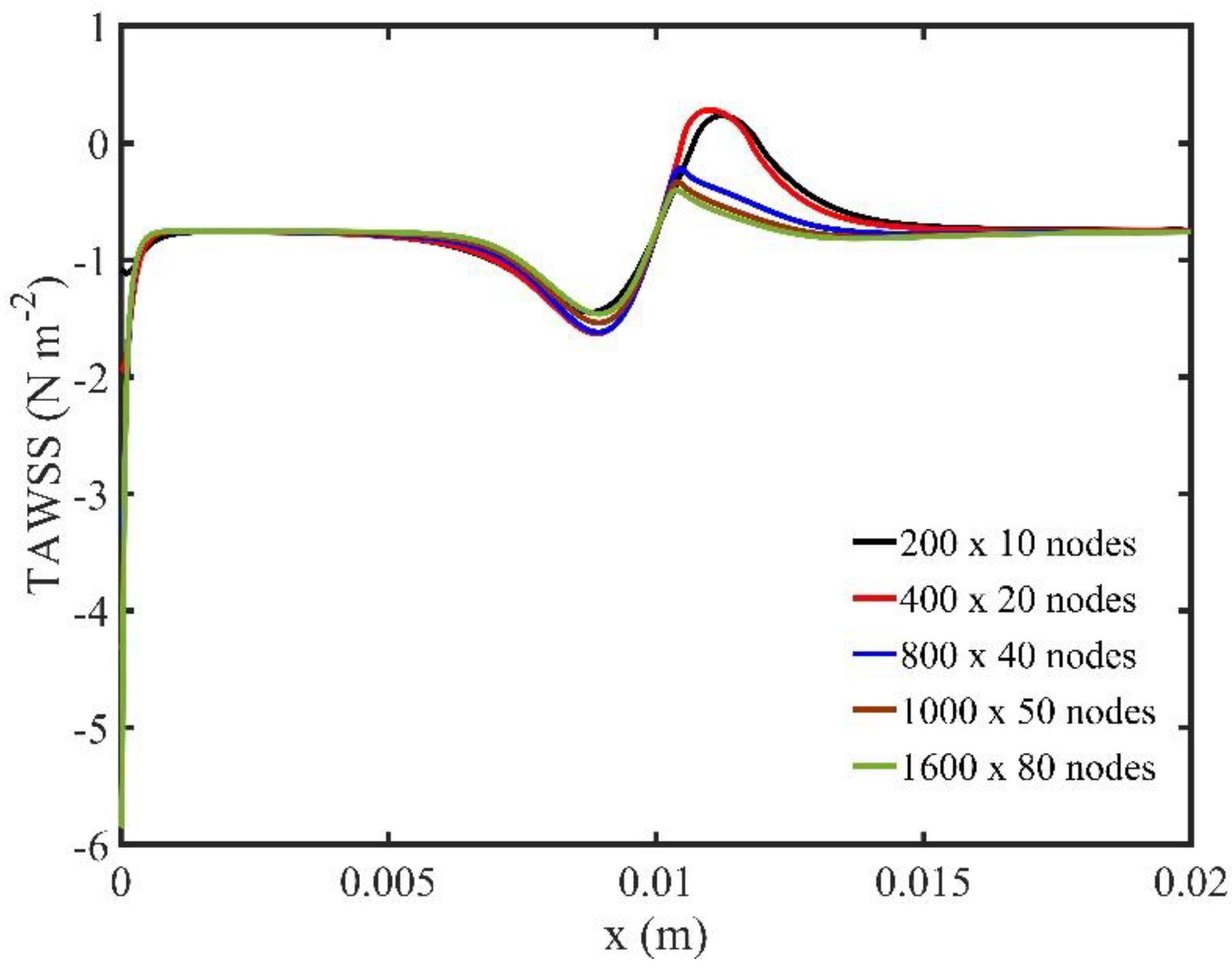
We demonstrate the convergence of the numerical method through a grid independence analysis study for all the flow cases considered. In this section, we present the convergence analysis study for the flow in a planar microchannel, the test case in the Section 4.1. The flow is laminar and non -Newtonian (following the Power-Law model). The density of the blood and MNPs are set to and , respectively. At the inlet of the microchannel, we set a pulsatile velocity profile [43]. Additionally, we apply a non-uniform magnetic field (generated by a wire carrying electric current) with magnetic field strength . The magnetic source is located at . The MNPs volume fraction is and their radius is .
We use successively denser grids and we examine the convergence of both stream function and vorticity field. Additionally, we examine the convergence of derived quantities, such as time average wall shear stress (TAWSS), which involves computation of spatial derivatives of the unknown field functions. We use five grid configurations, starting with a coarse grid with spatial resolution ( uniform grid with 2000 nodes in total), and a denser grid with resolution ( uniform grid and 128,000 nodes). Figure 1 shows the TAWSS for all grid configurations used. The difference for the two finest grids is less than 1%, indicating that the resolution higher than ensures a grid independent numerical solution.
We demonstrate the accuracy of the meshless method, by comparing the numerical results obtained with those reported in Loukopoulos and Tzirtzilakis [15], using the finite difference (FD) method. Figure 2 shows the velocity profile at computed using the MPC and the FD method [15].
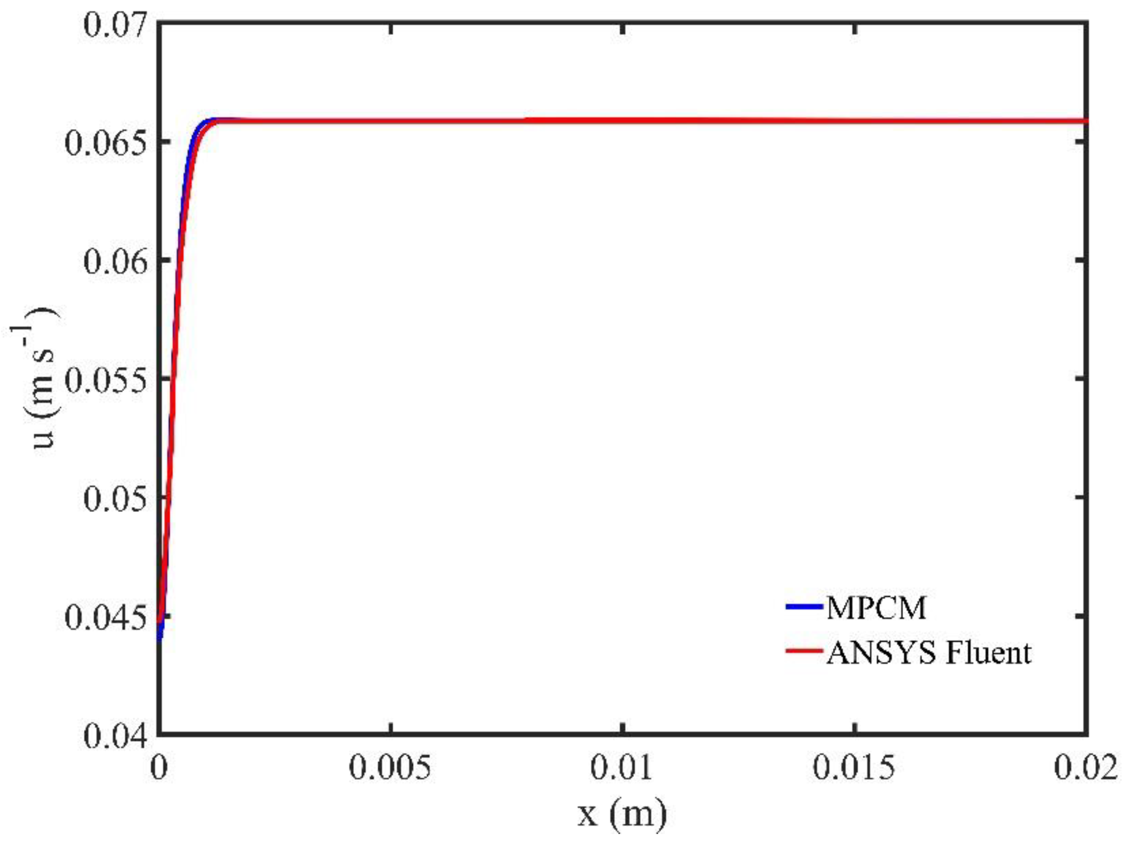
We also highlight the accuracy of our meshless scheme by comparing our time accurate solutions with those computed using the commercial CFD software ANSYS FLUENT® (ANSYS Inc., Canonsburg, PA, USA) [44]. The flow domain is a rectangular channel of length and width . The fluid flow is incompressible, laminar, non-Newtonian (power-law model with (Equation (16)). The density is set to and the viscosity to . We apply a sinusoidal velocity at the inlet. We compare the centerline velocity of the two methods for different time instances and the difference (for all three velocity vector components) is less than . Figure 3 shows a comparison of the two methods at time .
4. Results and Discussion
We numerically study MDT focusing on the flow regime and the concentration patterns of MNPs. For cardiovascular atherosclerosis, the therapeutic goal is to reduce the myocardial infraction and stabilize the atherosclerotic plaque. Biocompatible MNPs coated with drugs are navigated with a magnetic field to the atherosclerotic plaque.
In all flow cases considered, the flow is laminar and the blood is modeled as a non-Newtonian fluid using the power law viscosity model (Equation (17)), with material parameters values and (Equation (16)). Based on the experimental data in [23], viscosity obtains minimum and maximum values of and , respectively. We use the pulsatile velocity profile reported in [43]. The density of the blood and the MNPs is set to and [7], respectively. The radius of the MNPs, , is equal to .
We present results for different values of the solid volume fraction (), the magnetic field location ()—b is the vertical distance from the upper wall-, and the magnetic field strength (). We examine three flow geometries, namely a planar microchannel, a microchannel with stenosis and a microchannel with bifurcation.
We calculate the time average volume concentration ( where T is the time period of one cardiac cycle), and the time average wall shear stress (, where WSS is the instantaneous wall shear stress, that is, the force per unit area exerted by the fluid on the wall in a direction on the local tangent plane every time). The TAVC shows the distribution for non-dimensional concentration of the MNPs. We present results along the upper wall of microchannel, where the magnetic source is located. High values for TAVC demonstrate increased MNPs capture close to the magnetic source. A drawback of MDT is the increased likelihood for embolization, since nanoparticles accumulate and block the blood flow [45]. High values for TAWSS indicate a high velocity gradient and maximum shear stress [26]. In arterial blood flow the WSS, which is the frictional force acting on the endothelial cell surface due to blood flow, is considered to be a major factor for the early formation of an atherosclerotic plaque [45,46]. We present stream function contours to illustrate the effect of MNPs to the flow field, and to detect recirculation zones (vortices). Shear rate and flow recirculation zones are associated with distinct pathogenic and biological pathways relevant to atherogenesis and thrombosis [47].
4.1. MDT in a Planar Microchannel
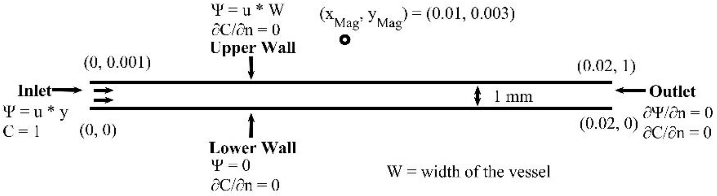
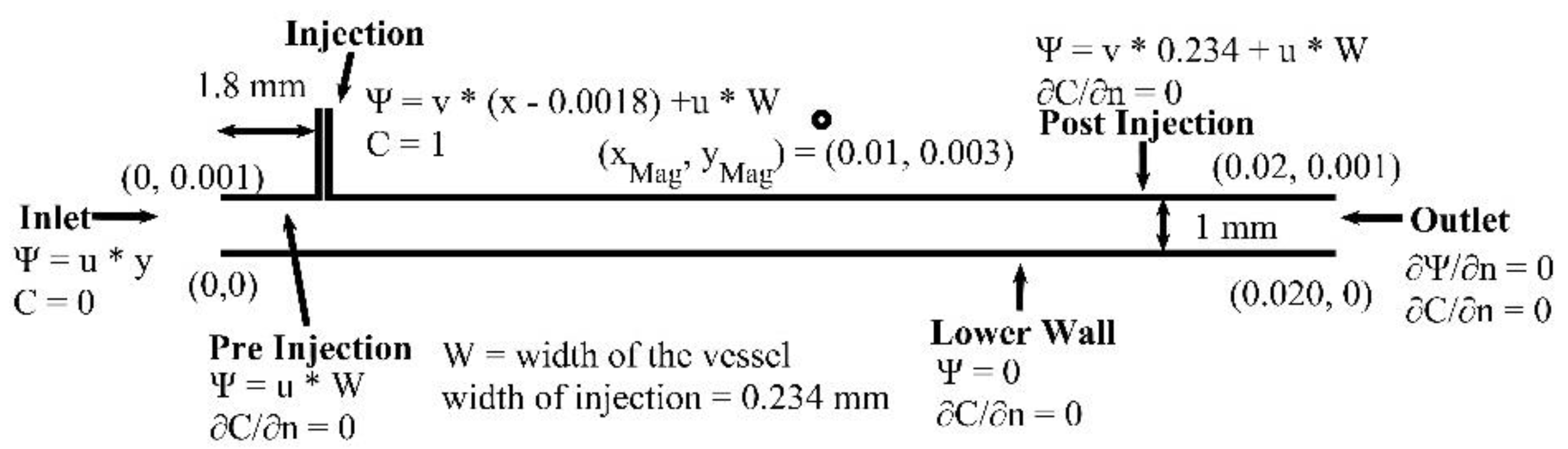
In this section, we study the biomagnetic flow in a planar microchannel. The flow domain and the boundary conditions are shown in Figure 5. The MNPs (drug carriers), enter the channel through the inlet. A detailed description of the concentration the boundary conditions is presented in [16,22]. We represent the spatial domain using 50,000 nodes, which ensure a grid independent numerical solution. We set the time step to s and the MNPs volume fraction at the inlet to φ = 0.03.
We examine the effects of varying volume fraction , distance of the magnetic field source from the upper wall of the microchannel, and magnetic field strength , affect the flow field, the distribution of dimensionless concentration along the upper wall, and the wall shear stress on the upper wall.
4.1.1. Effect of the MNPs Volume Fraction
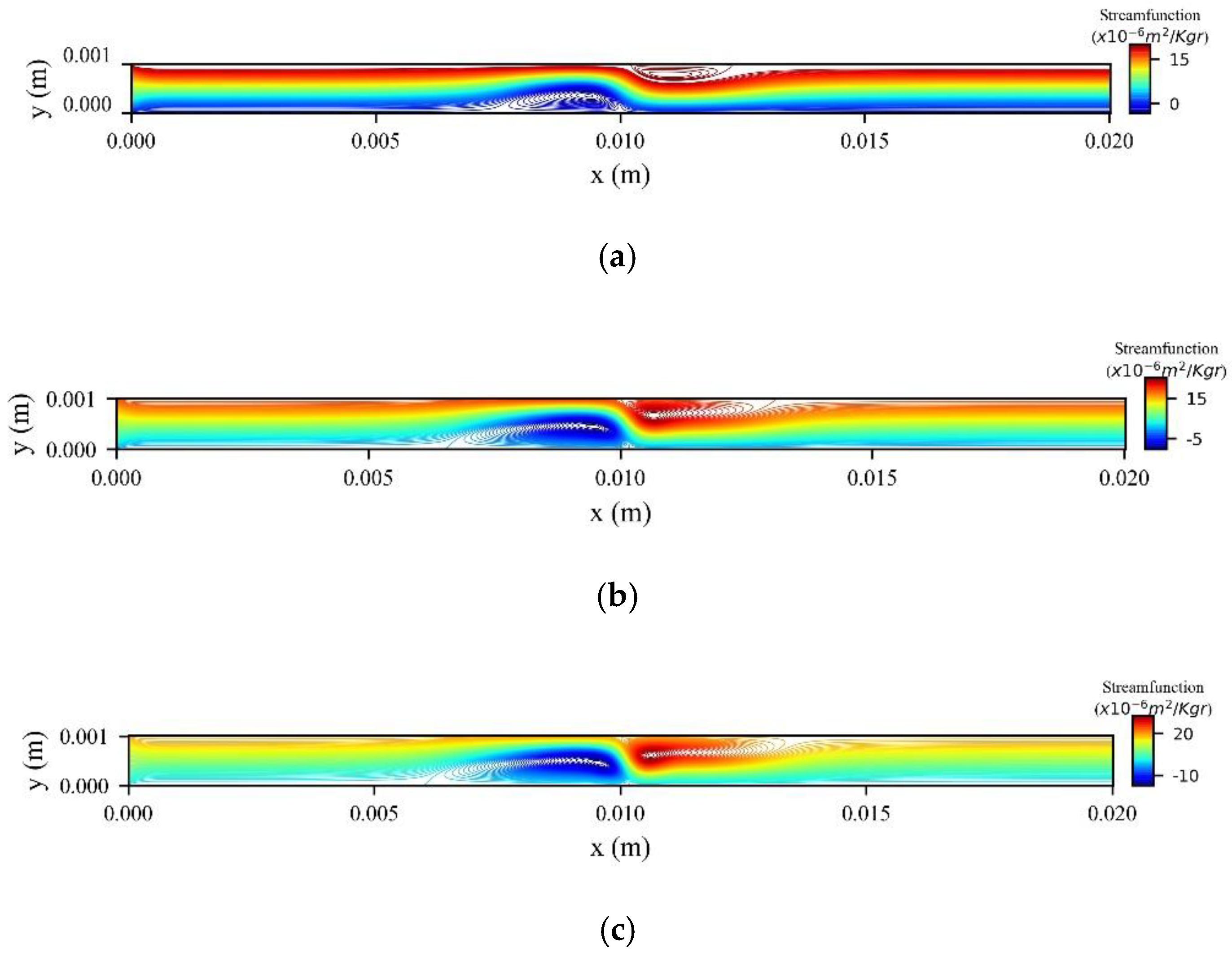
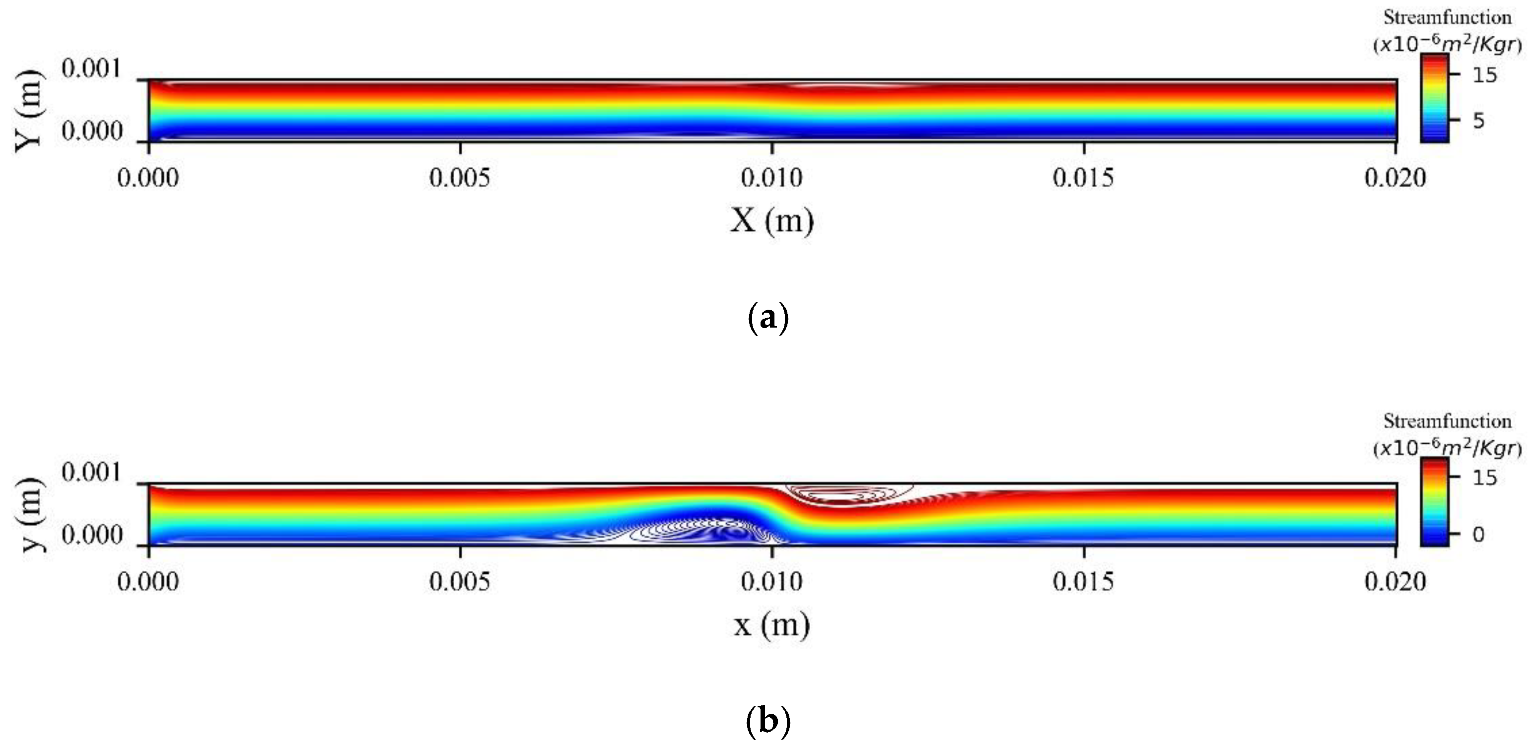
Figure 6 shows the stream function contours for different values of magnetic MNPs volume fraction at the peak systolic velocity (). The external magnetic field, with strength , is located at . We observe two vortices forming in the vicinity of the magnetic source. As increases both vortices increase in size and in strength.
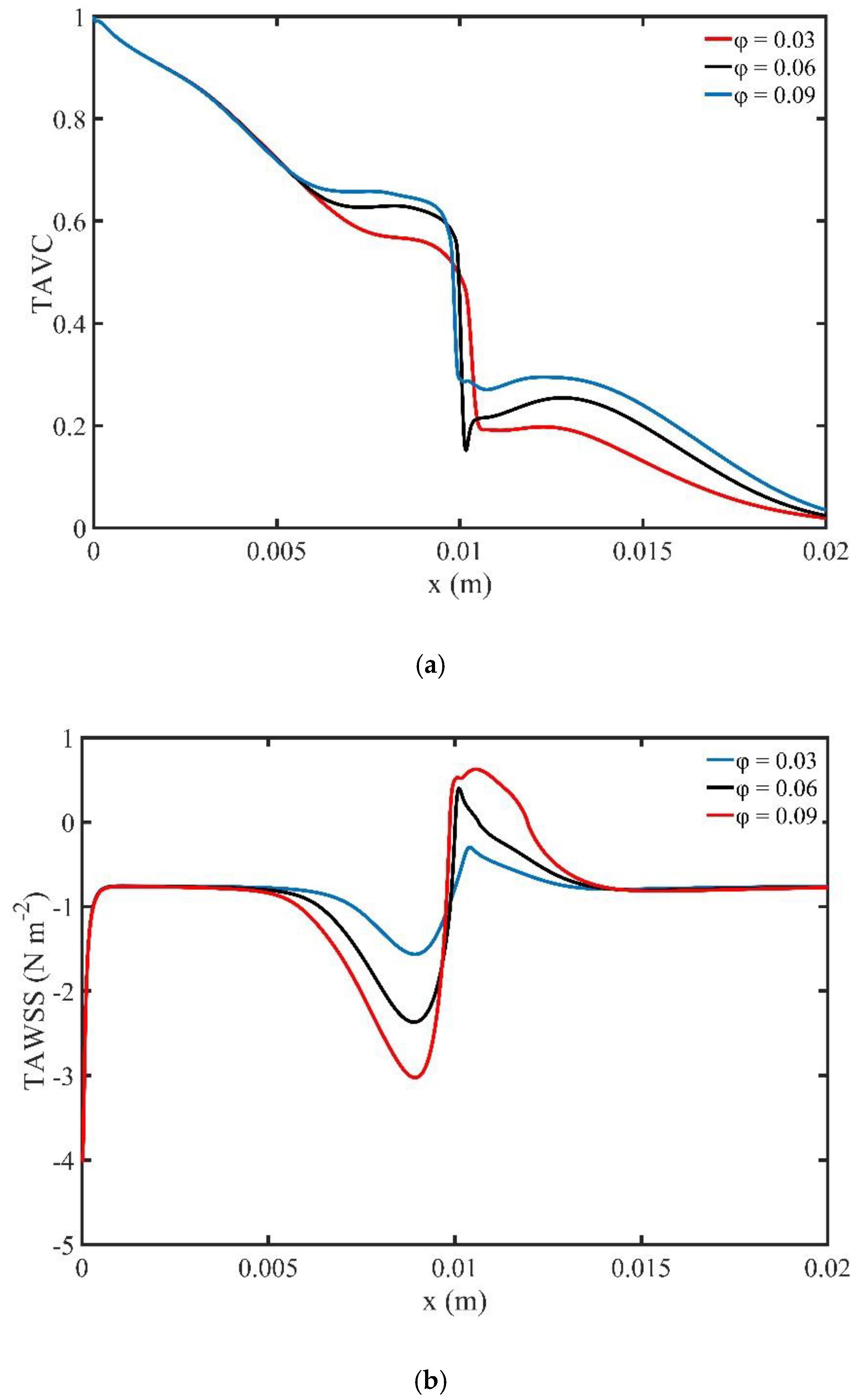
Figure 7a shows the variation of TAVC along the upper wall of microchannel versus volume fraction . We observe that as the volume fraction increases, there is an increase in the deposition of MNPs on the upper wall. Figure 7a shows a steep decrease of TAVC close to the magnetic source.
Figure 7b shows the TAWSS along the upper wall of the microchannel versus volume fraction . We observe elevated values of shear stress close to the magnetic source.
4.1.2. Effect of the Magnetic Field Location
We examined the effect of magnetic field location over the flow field and the distribution of MNPs non-dimensional concentration. The magnetic field source is located at three different positions above the midpoint of the upper wall and . The volume fraction (φ) of MNPs is set at the inlet.
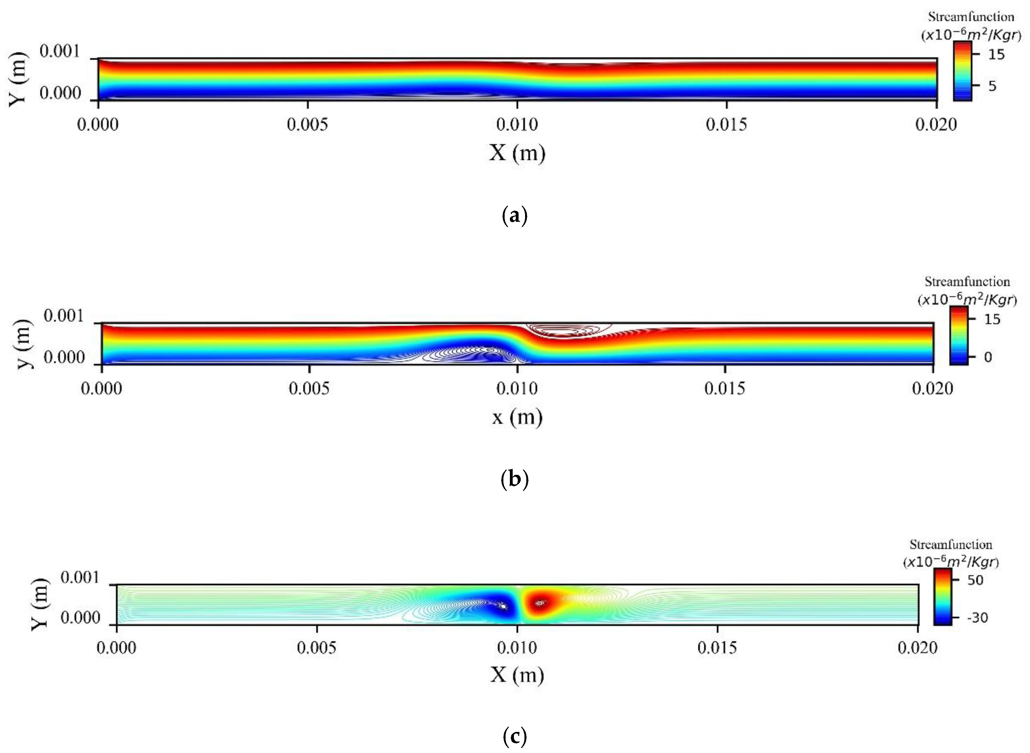
Figure 8 depicts the stream functions contours at the peak systolic velocity for t = 0.8 s. Strong recirculation zones, upstream and downstream of the location of the magnetic source are created for the two closest locations of the magnetic source. As the b increases, we observe that the magnitude of the disturbances decreases. For the effect of the magnetic field on the flow field is limited.
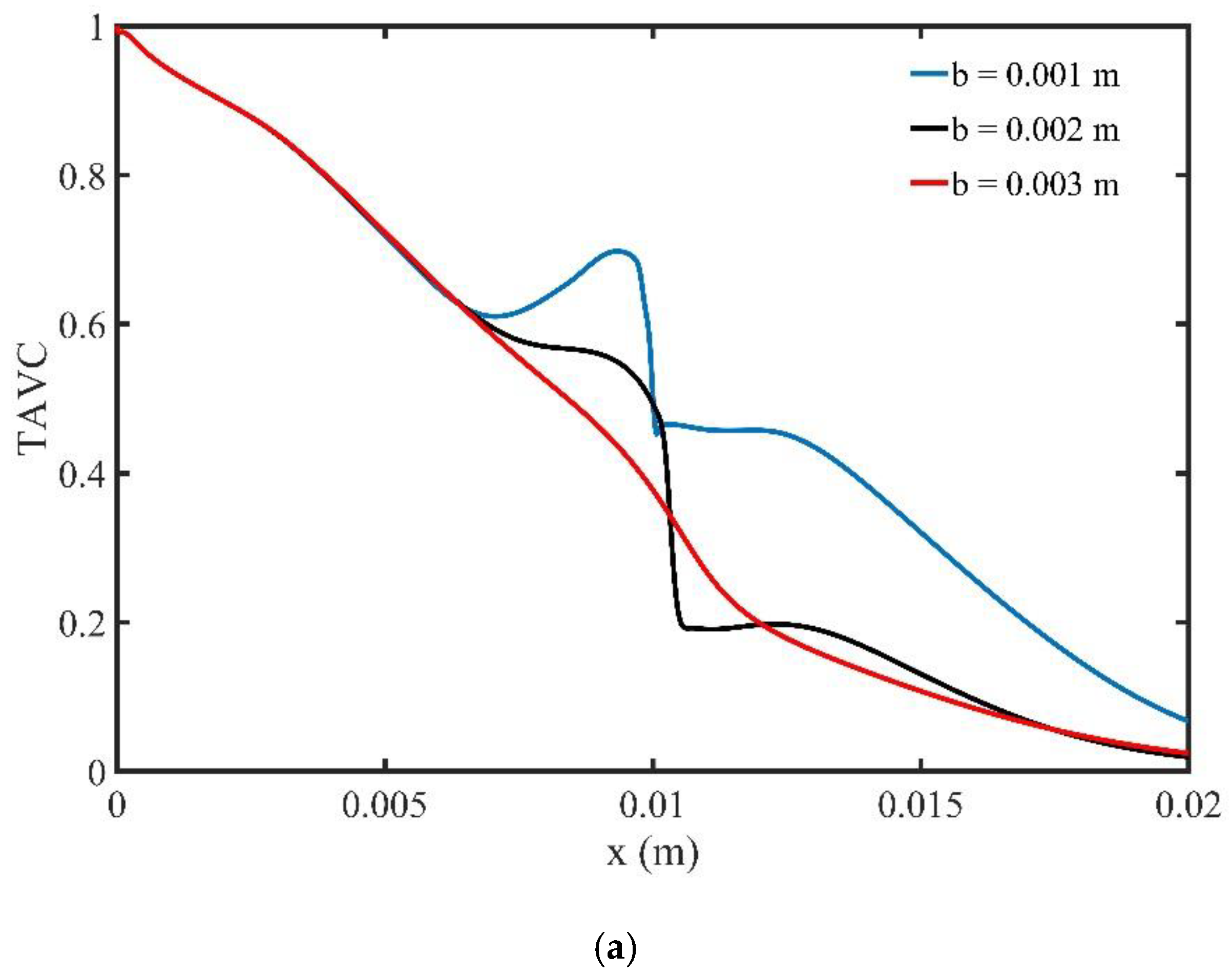
The profile of the TAVC along the upper wall of microchannel is shown in Figure 9a, for three specific locations of the magnetic field source. It is observed that when the magnetic field source is located closed to the upper wall, , there is an increase of TAVC upstream of the magnetic field source. Similar behavior of the TAVC of MNPs is followed when the distance b is increased, and , and thus the influence of the magnetic field is decreased. Figure 9b shows the effect of the magnetic field location on TAWSS. We observe that when the magnetic source is far from the upper wall of the channel, , the effect of the magnetic field on the TAWSS is negligible. When the distance is decreased, the TAWSS increases closed to the magnetic source. The highest TAWSS values are observed when the distance b is minimum and equal to .
4.1.3. Effect of the Magnetic Field Strength
Next, we examine the effect of the magnetic field strength and magnetic field gradients over the flow field and the distribution of MNPs non-dimensional concentration. The external, non-uniform magnetic field source is located at while the strength of the magnetic field takes values in the region (). The volume fraction of magnetic MNPs is set at the inlet.
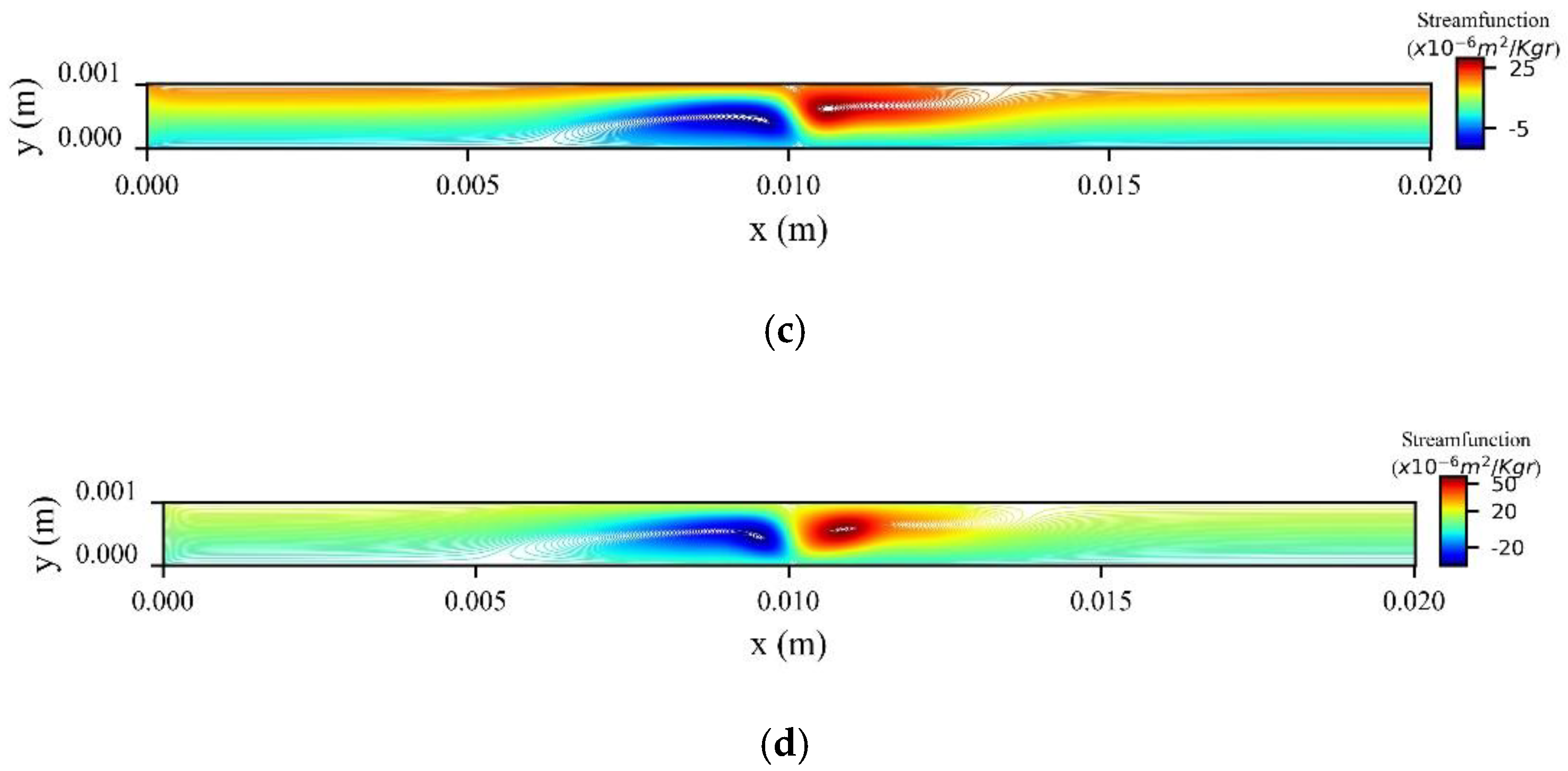
In Figure 10 we present the stream function contours for four values of the magnetic field strength γ at the peak systolic velocity when t = 0.8 s. The increase of the strength causes the formation of two recirculation zones (vortices) upstream and downstream the magnetic source. Moreover, the increase of γ increases the size and the strength of the vortices and thus causes further disturbances of the flow close to the magnetic source.
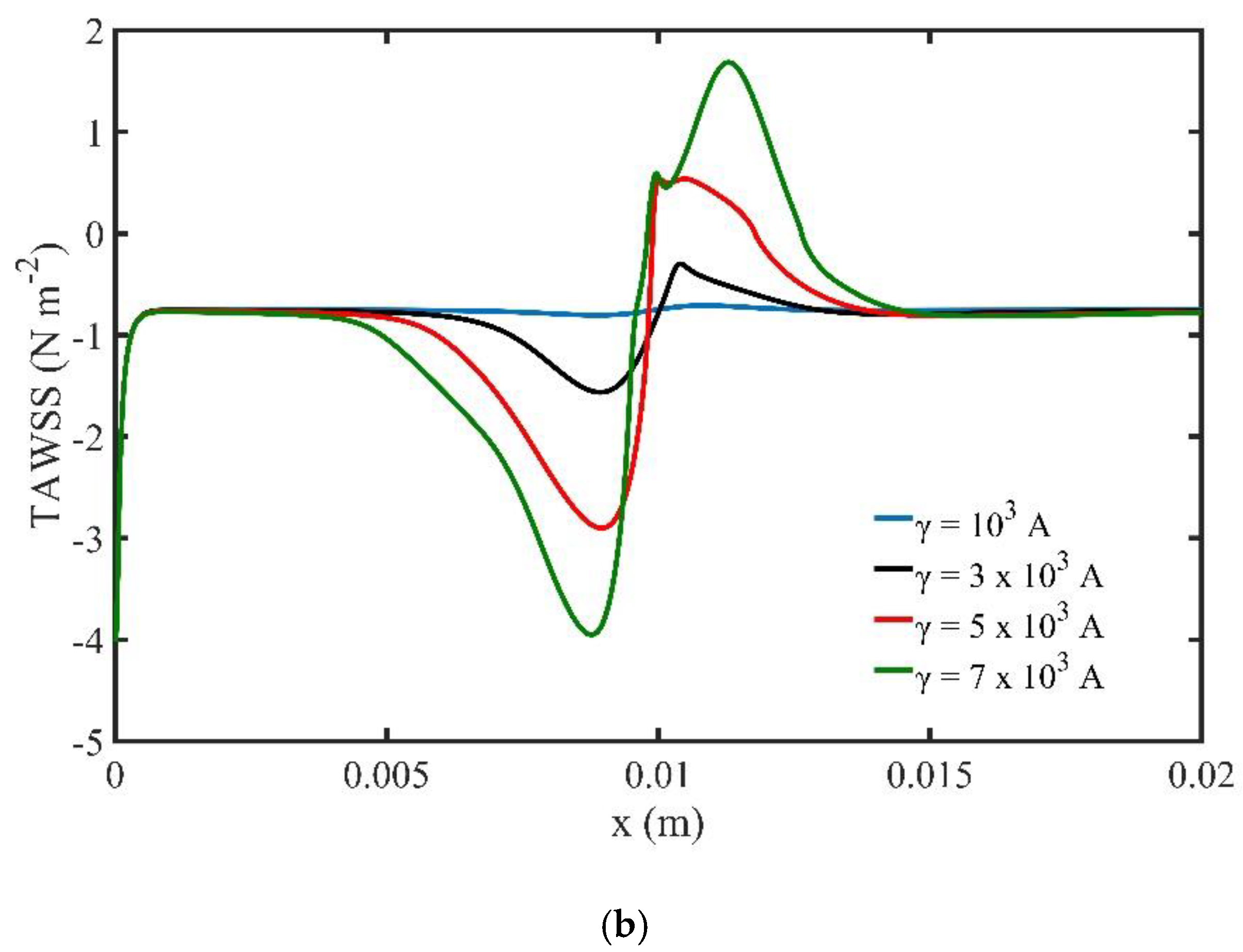
Figure 11a shows the variation of TAVC along the upper wall versus the intensity of the magnetic field γ for one period of the cardiac cycle. We observe that, when the strength of the magnetic field increases, the deposition of MNPs on the upper wall increase upstream the location of the magnetic field source. Moreover, the diagram shows a steep decrease of TAVC close to the magnetic source. The maximum TAVC value appears close to the magnetic source and is observed for the magnetic field strength . Figure 11b presents the TAWSS along the upper wall of the channel versus magnetic field strength. The strength of the magnetic field affects the TAWSS on the upper wall of the channel. Close to the magnetic source we observe high negative and positive levels of shear stresses. Higher levels of TAWSS can be noticed when the strength of the magnetic field increases.
4.2. MDT When MNPs Are Injected from the Upper Wall of the Microchannel
In this section, we investigate the MDT when MNPs are injected into the blood stream from the upper wall of microchannel. Figure 12 shows the flow domain and the boundary conditions.
We apply no-slip boundary conditions on the walls, and fully developed flow at the outlet (). At the inlet, we apply the flow waveform used in [43]. We apply Neumann boundary conditions at the walls and the outlet for the non-dimensional concentration. The MNPs are steadily injected with velocity in the blood stream, having a volume fraction of φ = 0.03 at the inlet. The cross-section area of the injection site is . The distance between the injection site and the inlet is . The magnetic source is located at , with magnetic field strength set to .
Figure 13 shows the distribution of the dimensionless concentration of MNPs in the vessel for various times during a cardiac cycle. When injection begins, it takes about before the MNPs approach the targeted tissue. The concentration close to the targeted tissue increases during the cardiac cycle when the velocity decreases. As a consequence, MNPs create an obstacle in front of the targeted tissue, and this obstacle is removed at the systole time when the hydrodynamic forces overcome the magnetic forces.
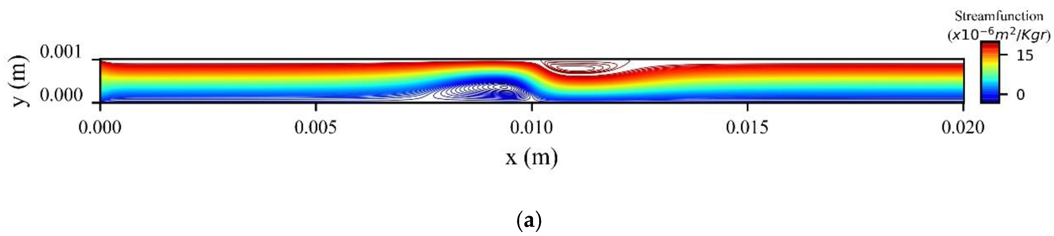
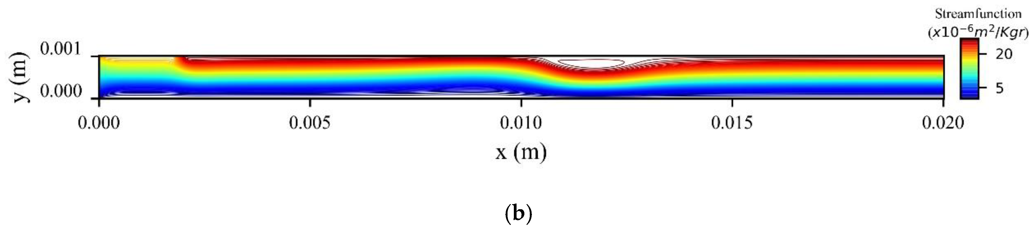
Figure 14a shows the stream function contours computed at the peak systolic velocity () when MNPs enter the microchannel from the inlet, while Figure 14b when the MNPs are injected from the upper wall. In the former, two recirculation zones (vortices) are formed upstream and downstream to the magnetic source, while in the latter only one recirculation zone (vortex) is formed upstream the magnetic source at the upper wall.
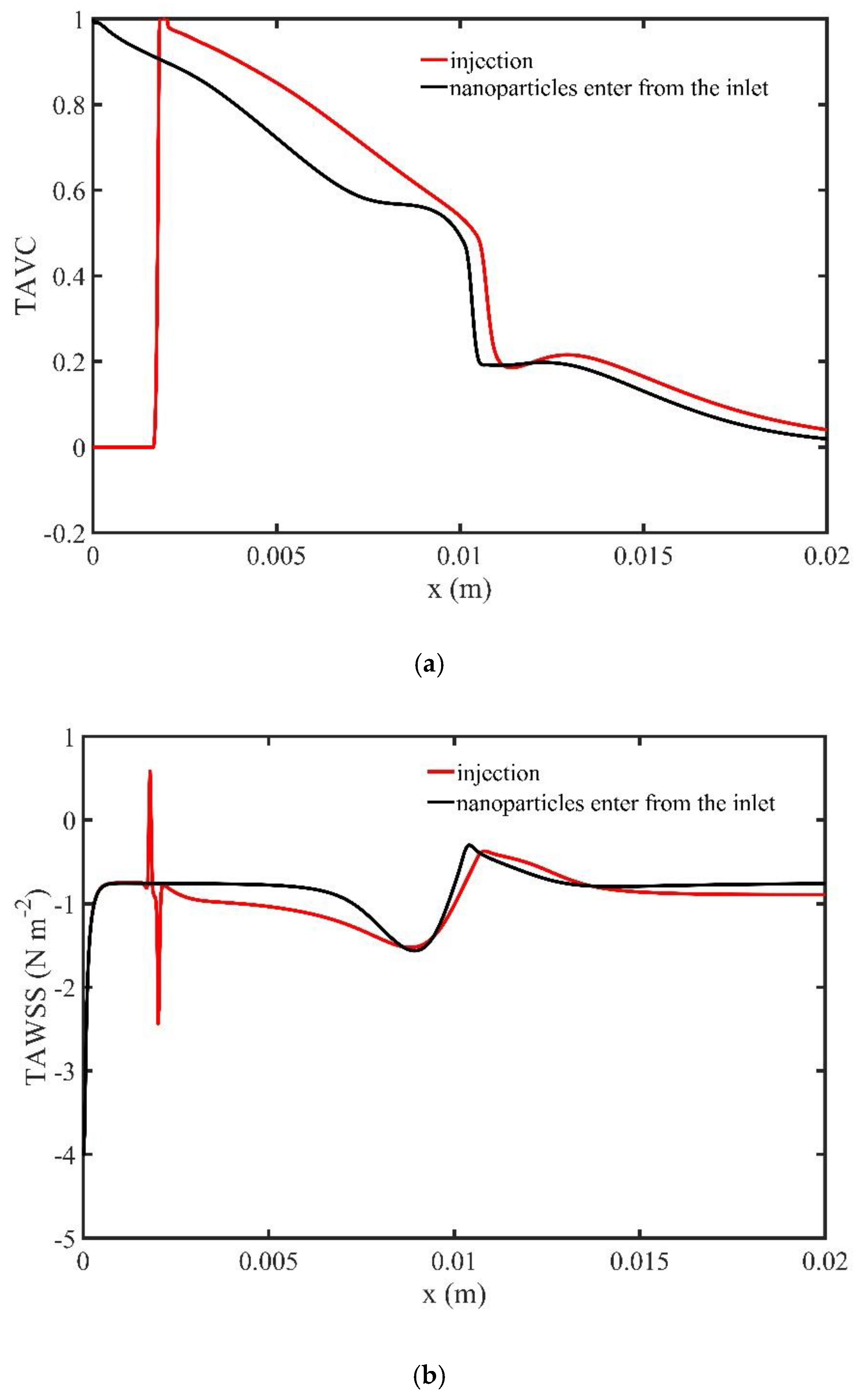
Figure 15a shows the variation of TAVC along the upper wall for a time period of one cardiac cycle for the two ways by which the MNPs approach the targeted tissue. The values of TAVC are higher when the second way is used. Figure 15b presents the TAWSS along the upper wall of the microchannel for one period of the cardiac cycle for the two ways by which the MNPs approach the targeted tissue. We observe minor differences for the values of TAWSS for the two approaches.
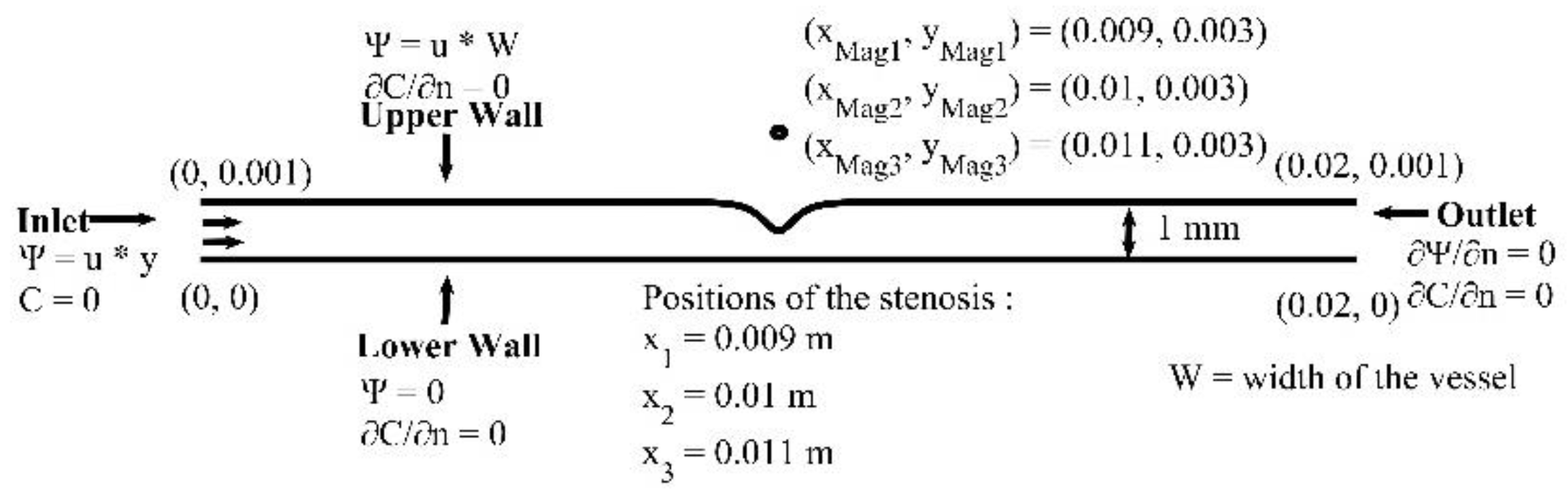
4.3. MDT in a Microchannel with Stenosis
In this section, we investigate the biomagnetic fluid flow in a microchannel with a stenosis located in the middle of the upper wall. We set the volume fraction of MNPs, entering at the inlet, to , the strength of the external magnetic field and the magnetic source in a distance above the upper wall. We change the horizontal coordinate for the magnetic source location to (in front of the stenosis), (in the middle of the stenosis) and (after the stenosis). We use a grid of approximately 58,000 nodes, that ensures a grid independent numerical solution. The time step was set to s. The geometry and the boundary conditions of the problem are presented in Figure 16.
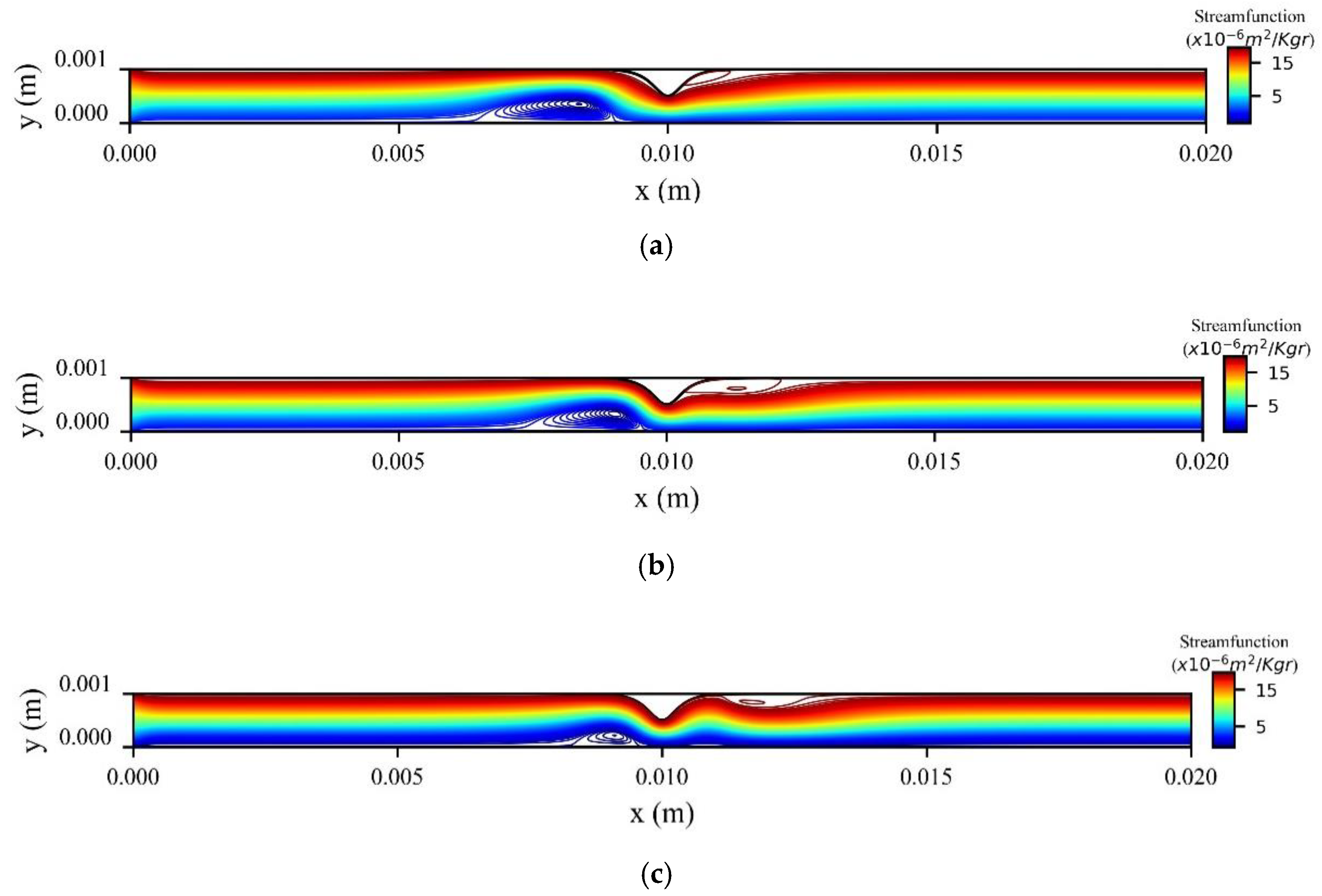
The stream function contours are presented in Figure 17 for three values of horizontal position of the magnetic source at the peak systolic velocity when t = 0.8 s. We see that two recirculation zones (vortices) are formed upstream and downstream of the stenosis. As the magnetic source is shifted from the left side to the right side of the stenosis, the first vortex is minimized, and the second vortex is enlarged.
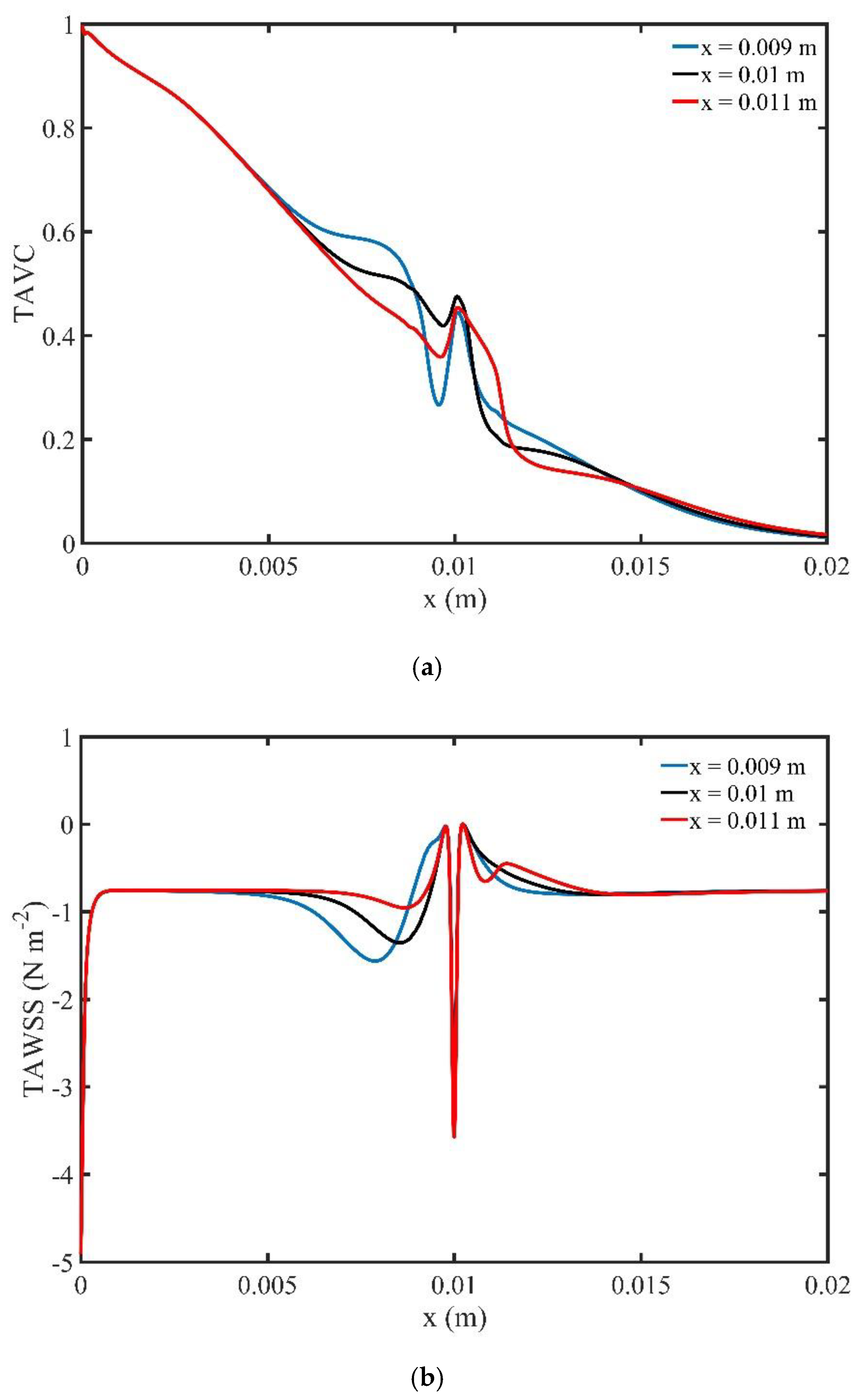
The profile of TAVC along the upper wall for one period of cardiac cycle is shown in Figure 18a. As the magnetic source is shifted towards the right, we observe variations of the TAVC which are located before and after the stenosis. Figure 18b presents the TAWSS along the upper wall of the microchannel for one period of cardiac cycle. The main differences for the three different positions of the magnetic field are found before the stenosis. In the middle of the upper wall of the channel where the stenosis is formed, we observe high levels of shear stresses for the three cases.
4.4. MDT in a Microchannel with Bifurcation
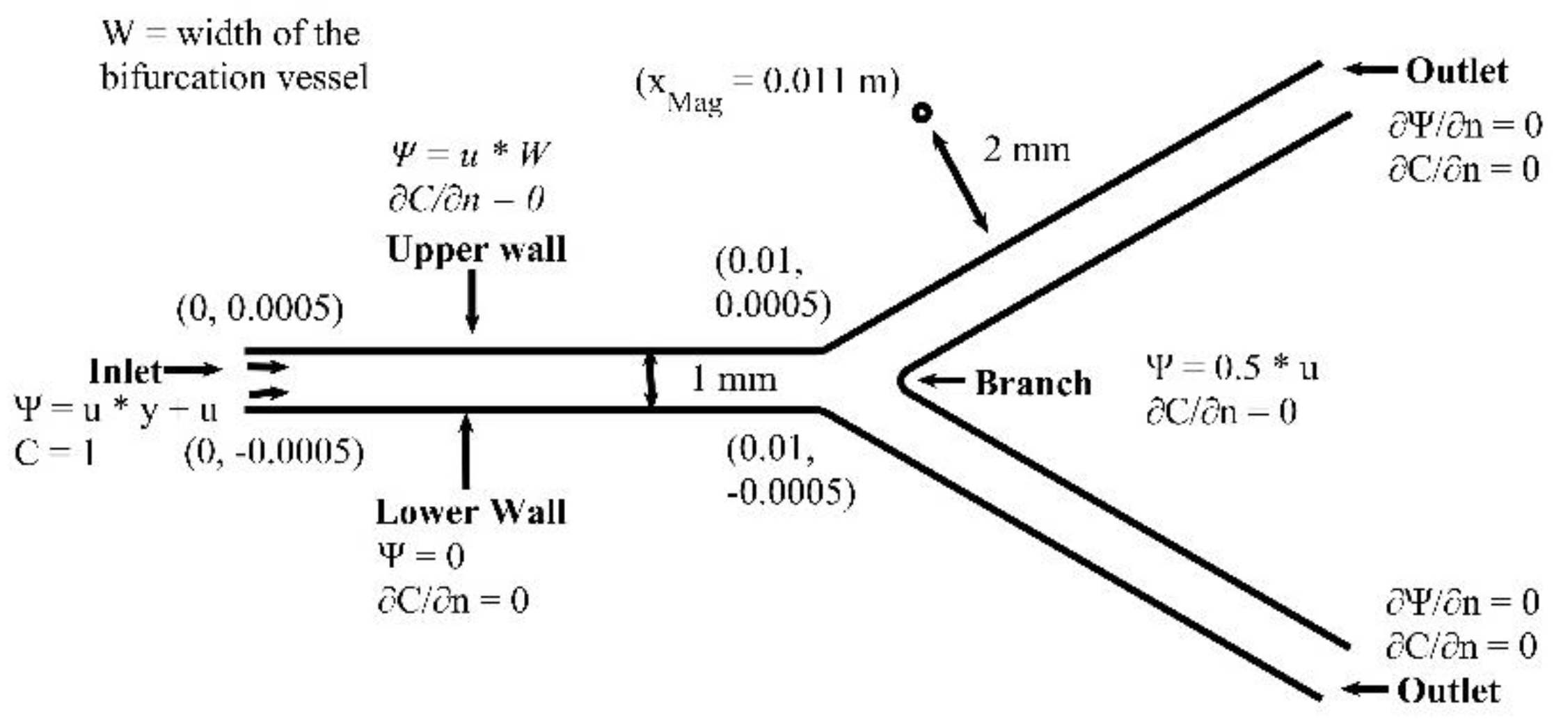
The branching angle and the diameter ratio in epicardial coronary artery bifurcations are two important factors of atherogenesis [46]. In this section, we examine the effect of different branching angle () of the bifurcation vessel on the MNPs concentration and the flow field. We present numerical results for the MDT biomagnetic (blood and dispersed MNPs) fluid flow in a microchannel (vessel) with bifurcation. Details on the geometry and the boundary conditions are in Figure 19. We set the MNPs volume fraction to , and the intensity of the external magnetic field to . The magnetic field is located at . We simulate two cardiac cycles. We use a grid of 120,000 nodes, which ensures a grid independent numerical solution. The time step was set to s.
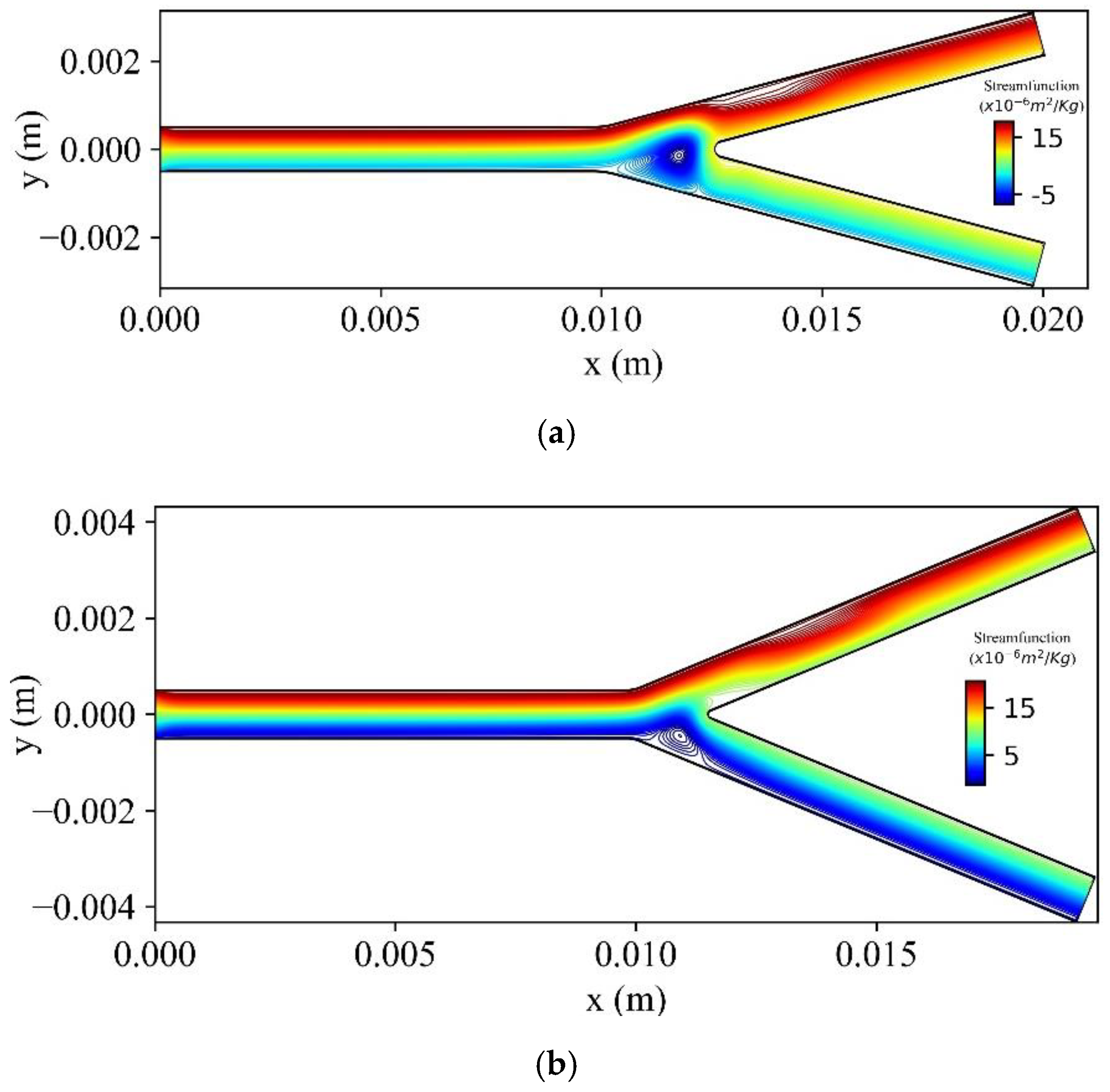
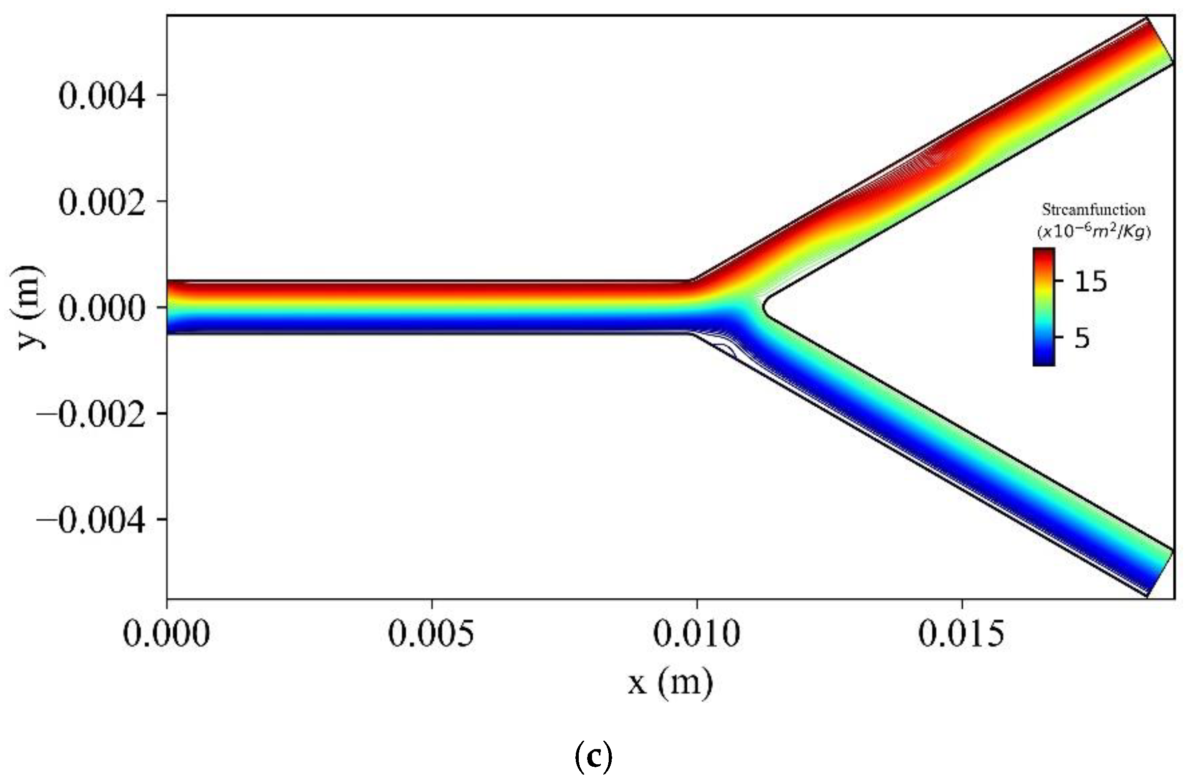
Figure 20 shows the stream function contours for three bifurcation angles (, , ) at t = 1.6 s. As the bifurcation angle decreases, a vortex is generated at the lower wall of the bifurcation.
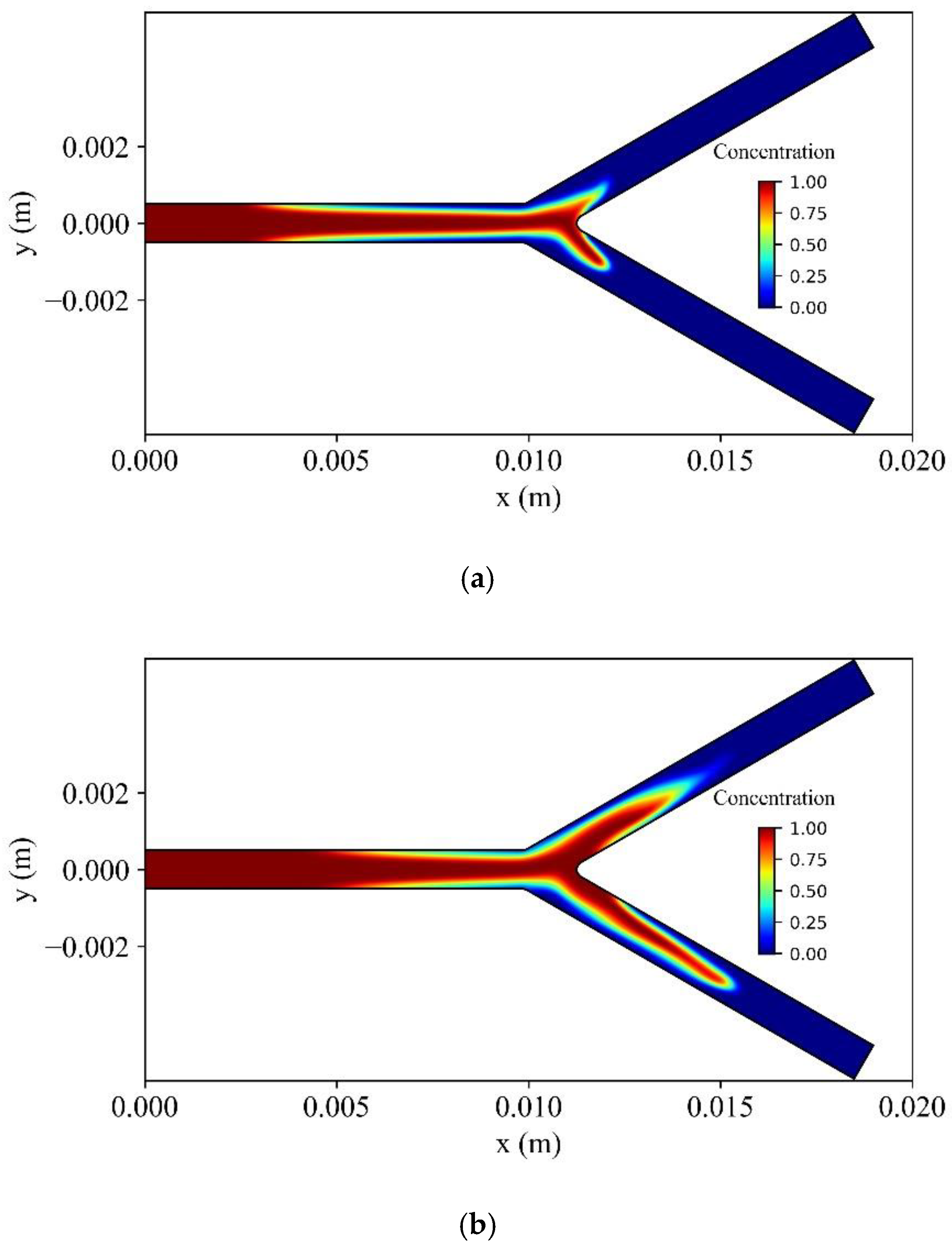
Figure 21 shows the distribution of the dimensionless concentration of MNPs in the vessel at different time instances. At the upper branch wall of the bifurcation, the MNPs capture is increased, causing a delay for MNPs to wash out at the outlet of the upper branch. The opposite is observed at the lower branch of the bifurcation, where the intensity of the magnetic field is weaker.
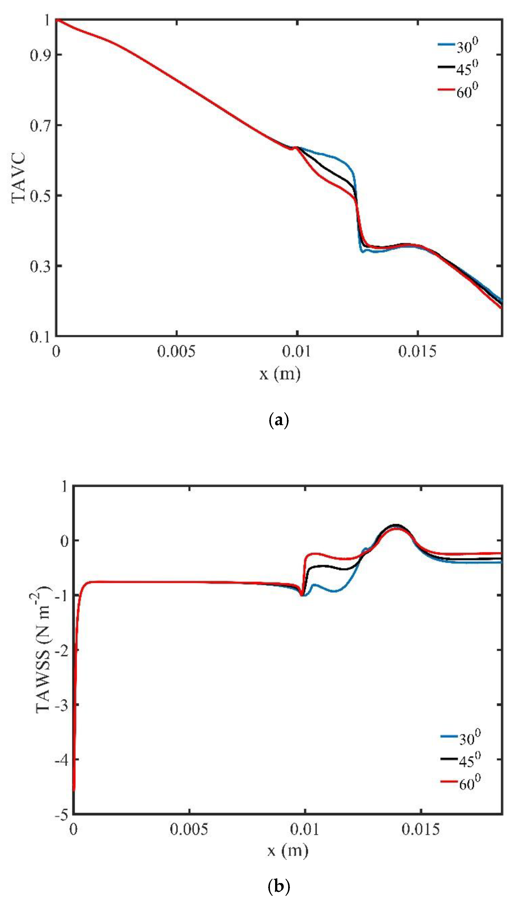
Figure 22a shows the variation of the TAVC along the upper wall of the bifurcation for various bifurcation angles. We observe that as the bifurcation angle decreases, there is an increase of TAVC of the magnetic field source. Finally, Figure 22b shows the variation of the TAWSS along the upper wall of the three bifurcations. The bifurcation angle affects the TAWSS upstream of the magnetic source, while downstream of the magnetic source the TAWSS maintains their values to the same order of magnitude.
5. Conclusions
We presented a numerical model to investigate the MDT flow problem. We examined the concentration distribution of MNPs under the presence of an external non-uniform magnetic field. The flow model used in the MDT flow simulation was based on the principles of FHD and BFD. The bio-magnetic fluid (blood and dispersed -MNPs) was modeled as two-phase, non-Newtonian fluid and the flow as pulsatile and laminar. The following key points were derived:
- MNPs loaded with medicinal drugs can be carried to a tissue target in the human body under the applied magnetic field.
- Recirculation zones are formed upstream and downstream of the targeting area (which is near to the location of the magnetic field), as the volume fraction of MNPs increases.
- The capture of MNPs on the tissue target increases with the volume fraction of MNPs and high values of the TAWSS are presented.
- When the magnetic source is placed close to the tissue target, recirculation zones are formed upstream and downstream of the targeting area.
- The increase of the strength of magnetic field causes the increase of TAWSS close to the tissue target.
- The MDT flow case in a microchannel with bifurcation shows that the decrease of the bifurcation angle results to the formation of one recirculation zone at the lower branch of the bifurcation, while at the upper branch, MNPs capture is larger.
Author Contributions
Conceptualization, I.D.B. and V.C.L.; methodology, I.D.B. and V.C.L.; validation, I.D.B. and G.C.B.; investigation, I.D.B., D.S.L., and V.C.L.; software, I.D.B., D.S.L., and V.C.L.; writing—original draft preparation, I.D.B. and V.C.L.; writing—review and editing, I.D.B., D.S.L., G.C.B., K.M., and V.C.L.; supervision, V.C.L. and K.M. All authors have read and agreed to the published version of the manuscript.
Funding
This research is co-financed by Greece and the European Union (European Social Fund- ESF) through the Operational Program «Human Resources Development, Education and Lifelong Learning» in the context of the project “Strengthening Human Resources Research Potential via Doctorate Research” (MIS-5000432), implemented by the State Scholarships Foundation (ΙΚΥ). This research was supported in part by the Australian Government through the Australian Research Council’s Discovery Projects funding scheme (project DP160100714). The views expressed herein are those of the authors and are not necessarily those of the Australian Research Council.
Conflicts of Interest
The authors declare no conflict of interest.
References
- Matoba, T.; Egashira, K. Nanoparticle-mediated drug delivery system for cardiovascular disease. Int. Heart J. 2014, 55, 281–286. [Google Scholar] [CrossRef] [PubMed] [Green Version]
- Sun, C.; Lee, J.S.; Zhang, M. Magnetic nanoparticles in MR imaging and drug delivery. Adv. Drug Deliv. Rev. 2008, 60, 1252–1265. [Google Scholar] [CrossRef] [PubMed] [Green Version]
- Cheraghi, M.; Negahdari, B.; Daraee, H.; Eatemadi, A. Heart targeted nanoliposomal/nanoparticles drug delivery: An updated review. Biomed. Pharmacother. 2017, 86, 316–323. [Google Scholar] [CrossRef] [PubMed]
- Schiener, M.; Hossann, M.; Viola, J.R.; Ortega-Gomez, A.; Weber, C.; Lauber, K.; Soehnlein, O. Nanomedicine-based strategies for treatment of atherosclerosis. Trends Mol. Med. 2014, 20, 271–281. [Google Scholar] [CrossRef]
- Carla, A.H. Dendritic supramolecular assemblies for drug delivery. Chem. Commun. 2005, 34, 4309–4311. [Google Scholar]
- Wilczewska, A.Z.; Niemirowicz, K.; Markiewicz, K.H.; Car, H. Nanoparticles as drug delivery systems. Pharmacol. Rep. 2012, 64, 1020–1037. [Google Scholar] [CrossRef]
- Teja, A.S.; Koh, P.Y. Synthesis, properties, and applications of magnetic iron oxide nanoparticles. Prog. Cryst. Growth Charact. Mater. 2009, 55, 22–45. [Google Scholar] [CrossRef]
- McNamara, K.; Tofail, S.A. Nanoparticles in biomedical applications. Adv. Phys. X 2017, 2, 54–88. [Google Scholar] [CrossRef]
- Cornell, R.M.; Schwertmann, U. Introduction to the iron oxides. Iron Oxides 2004, 1–7. [Google Scholar] [CrossRef]
- Kao, C.W.; Wu, P.T.; Liao, M.Y.; Chung, I.J.; Yang, K.C.; Tseng, W.Y.I.; Yu, J. Magnetic nanoparticles conjugated with peptides derived from monocyte chemoattractant protein-1 as a tool for targeting atherosclerosis. Pharmaceutics 2018, 10, 62. [Google Scholar] [CrossRef] [Green Version]
- Kudr, J.; Haddad, Y.; Richtera, L.; Heger, Z.; Cernak, M.; Adam, V.; Zitka, O. Magnetic nanoparticles: From design and synthesis to real world applications. Nanomaterials 2017, 7, 243. [Google Scholar] [CrossRef] [PubMed]
- Chatterjee, K.; Sarkar, S.; Rao, K.J.; Paria, S. Core/shell nanoparticles in biomedical applications. Adv. Colloid Interface Sci. 2014, 209, 8–39. [Google Scholar] [CrossRef] [PubMed]
- McCarthy, J.R.; Weissleder, R. Multifunctional magnetic nanoparticles for targeted imaging and therapy. Adv. Drug Deliv. Rev. 2008, 60, 1241–1251. [Google Scholar] [CrossRef] [PubMed] [Green Version]
- Haik, Y.; Pai, V.; Chen, C.J. Development of magnetic device for cell separation. J. Magn. Magn. Mater. 1999, 194, 254–261. [Google Scholar] [CrossRef]
- Loukopoulos, V.C.; Tzirtzilakis, E.E. Biomagnetic channel flow in spatially varying magnetic field. Int. J. Eng. Sci. 2004, 42, 571–590. [Google Scholar] [CrossRef]
- Khashan, S.A.; Elnajjar, E.; Haik, Y. Numerical simulation of the continuous biomagnetic separation in a two-dimensional channel. Int. J. Multiph. Flow 2011, 37, 947–955. [Google Scholar] [CrossRef]
- Rosensweig, R.E. Ferrohydrodynamics; Courier Corporation: Chelmsford, MA, USA, 2013. [Google Scholar]
- Neuringer, J.L.; Rosensweig, R.E. Ferrohydrodynamics. Phys. Fluids 1964, 7, 1927–1937. [Google Scholar] [CrossRef]
- Rosensweig, R.E. Magnetic fluids. Annu. Rev. Fluid Mech. 1987, 19, 437–461. [Google Scholar] [CrossRef]
- Tzirtzilakis, E.E.; Loukopoulos, V.C. Biofluid flow in a channel under the action of a uniform localized magnetic field. Comput. Mech. 2005, 36, 360–374. [Google Scholar] [CrossRef]
- Tzirtzilakis, E.E. Biomagnetic fluid flow in a channel with stenosis. Phys. D Nonlinear Phenom. 2008, 237, 66–81. [Google Scholar] [CrossRef]
- Khashan, S.A.; Elnajjar, E.; Haik, Y. CFD simulation of the magnetophoretic separation in a microchannel. J. Magn. Magn. Mater. 2011, 323, 2960–2967. [Google Scholar] [CrossRef]
- Habibi, M.R.; Ghassemi, M.; Hamedi, M.H. Analysis of high gradient magnetic field effects on distribution of nanoparticles injected into pulsatile blood stream. J. Magn. Magn. Mater. 2012, 324, 1473–1482. [Google Scholar] [CrossRef]
- Habibi, M.R.; Ghasemi, M. Numerical study of magnetic nanoparticles concentration in biofluid (blood) under influence of high gradient magnetic field. J. Magn. Magn. Mater. 2011, 323, 32–38. [Google Scholar] [CrossRef]
- Bose, S.; Banerjee, M. Magnetic particle capture for biomagnetic fluid flow in stenosed aortic bifurcation considering particle–fluid coupling. J. Magn. Magn. Mater. 2015, 385, 32–46. [Google Scholar] [CrossRef]
- Larimi, M.M.; Ramiar, A.; Ranjbar, A.A. Numerical simulation of magnetic nanoparticles targeting in a bifurcation vessel. J. Magn. Magn. Mater. 2014, 362, 58–71. [Google Scholar] [CrossRef]
- Khashan, S.A.; Furlani, E.P. Coupled particle–fluid transport and magnetic separation in microfluidic systems with passive magnetic functionality. J. Phys. D Appl. Phys. 2013, 46, 125002. [Google Scholar] [CrossRef]
- Li, X.L.; Yao, K.L.; Liu, Z.L. CFD study on the magnetic fluid delivering in the vessel in high-gradient magnetic field. J. Magn. Magn. Mater. 2008, 320, 1753–1758. [Google Scholar] [CrossRef]
- Hoffmann, K.A.; Chiang, S.T. Computational fluid dynamics volume I. Engineering Education System. Available online: https://www.twirpx.com/file/412383/ (accessed on 27 May 2020).
- Khanafer, K.; Vafai, K.; Lightstone, M. Buoyancy-driven heat transfer enhancement in a two-dimensional enclosure utilizing nanofluids. Int. J. Heat Mass Transf. 2003, 46, 3639–3653. [Google Scholar] [CrossRef]
- Haik, Y.; Pai, V.; Chen, C.J. Apparent viscosity of human blood in a high static magnetic field. J. Magn. Magn. Mater. 2001, 225, 180–186. [Google Scholar] [CrossRef]
- Tzirtzilakis, E.E. A mathematical model for blood flow in magnetic field. Phys. Fluids 2005, 17, 077103. [Google Scholar] [CrossRef]
- Berthier, J.; Silberzan, P.; Berthier, J.; Silberzan, P. Microfluidics for Biotechnology; Artech House: Norwood, MA, USA, 2010. [Google Scholar]
- Johnston, B.M.; Johnston, P.R.; Corney, S.; Kilpatrick, D. Non-Newtonian blood flow in human right coronary arteries: Steady state simulations. J. Biomech. 2004, 37, 709–720. [Google Scholar] [CrossRef] [Green Version]
- Cregg, P.J.; Murphy, K.; Mardinoglu, A.; Prina-Mello, A. Many particle magnetic dipole–dipole and hydrodynamic interactions in magnetizable stent assisted magnetic drug targeting. J. Magn. Magn. Mater. 2010, 322, 2087–2094. [Google Scholar] [CrossRef]
- Cregg, P.J.; Murphy, K.; Mardinoglu, A. Inclusion of interactions in mathematical modelling of implant assisted magnetic drug targeting. Appl. Math. Model. 2012, 36, 1–34. [Google Scholar] [CrossRef]
- Liu, G.R. Meshfree Methods: Moving beyond the Finite Element Method; Taylor & Francis: Oxford Shire, UK, 2009. [Google Scholar]
- Bourantas, G.C.; Loukopoulos, V.C. Modeling the natural convective flow of micropolar nanofluids. Int. J. Heat Mass Transf. 2014, 68, 35–41. [Google Scholar] [CrossRef]
- Bourantas, G.; Skouras, E.; Loukopoulos, V.; Nikiforidis, G. Meshfree point collocation schemes for 2d steady state incompressible navier-stokes equations in velocity-vorticity formulation for high values of reynolds number. Comput. Modeling Eng. Sci. 2010, 59, 31–63. [Google Scholar]
- Loukopoulos, V.C.; Bourantas, G.C.; Labropoulos, D.; Nikiforidis VM, G.; Bordas, S.; Nikiforidis, G.C. Numerical Study of Magnetic Particles Concentration in Biofluid (Blood) under the Influence of High Gradient Magnetic Field in Microchannel. In Proceedings of the European Congress on Computational Methods in Applied Sciences and Engineering, ECCOMAS Congress 2016, Crete Island, Greece, 5–10 June 2016; pp. 1084–1092. [Google Scholar]
- Bourantas, G.C.; Skouras, E.D.; Loukopoulos, V.C.; Nikiforidis, G.C. An accurate, stable and efficient domain-type meshless method for the solution of MHD flow problems. J. Comput. Phys. 2009, 228, 8135–8160. [Google Scholar] [CrossRef] [Green Version]
- Loukopoulos, V.C.; Bourantas, G.C.; Skouras, E.D.; Nikiforidis, G.C. Localized meshless point collocation method for time-dependent magnetohydrodynamics flow through pipes under a variety of wall conductivity conditions. Comput. Mech. 2011, 47, 137–159. [Google Scholar] [CrossRef] [Green Version]
- Ding, Z.R.; Bin, L.I.U.; Shuo, Y.A.N.G.; Yan, X.I.A. Hemodynamics for asymmetric inlet axial velocity profile in carotid bifurcation model. J. Hydrodyn. Ser. B 2008, 20, 656–661. [Google Scholar] [CrossRef]
- Kohnke, P. Theory Guide; ANSYS, Inc.: Canonsburg, PA, USA, 2013. [Google Scholar]
- Dobson, J. Magnetic nanoparticles for drug delivery. Drug Dev. Res. 2006, 67, 55–60. [Google Scholar] [CrossRef]
- Huo, Y.; Finet, G.; Lefevre, T.; Louvard, Y.; Moussa, I.; Kassab, G.S. Which diameter and angle rule provides optimal flow patterns in a coronary bifurcation? J. Biomech. 2012, 45, 1273–1279. [Google Scholar] [CrossRef] [Green Version]
- Javadzadegan, A.; Yong, A.S.; Chang, M.; Ng, A.C.; Yiannikas, J.; Ng, M.K.; Kritharides, L. Flow recirculation zone length and shear rate are differentially affected by stenosis severity in human coronary arteries. Am. J. Physiol.-Heart Circ. Physiol. 2013, 304, H559–H566. [Google Scholar] [CrossRef] [Green Version]
Figure 1.
Mesh independency study of the TAWSS on the upper wall of the vessel.

Figure 2.
Dimensionless velocity profile at the position .

Figure 3.
Centerline velocity profile of sinusoidal flow for .

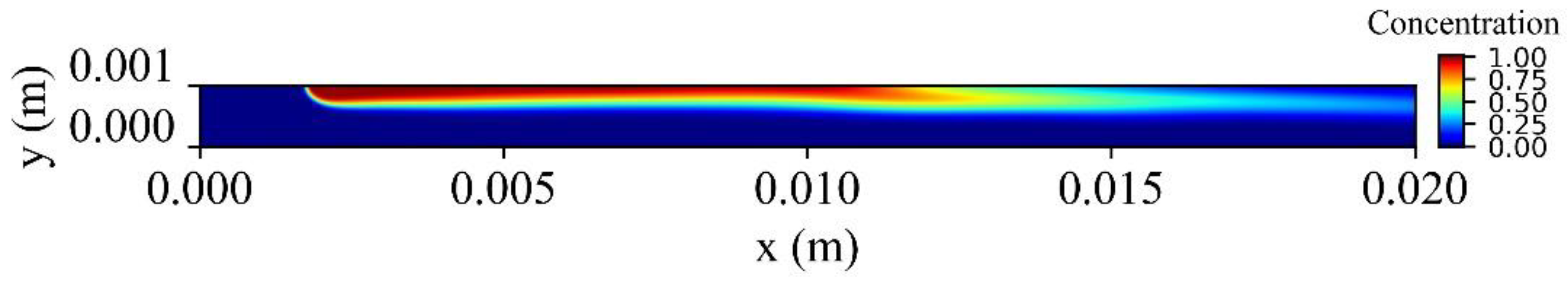
Figure 4.
Non dimensional concentration for 2000 nm MNPS’ diameter and average velocity 0.0281 ms−1 at time with MPC method.
Figure 4.
Non dimensional concentration for 2000 nm MNPS’ diameter and average velocity 0.0281 ms−1 at time with MPC method.

Figure 5.
Computational domain for planar microchannel, where the MNPs are inserted from the inlet.

Figure 6.
Stream function contours for (a) φ, (b) φ , and (c) φ at

Figure 7.
(a) Time average volume concentration (TAVC) and (b) Time average wall shear stress (TAWSS), along the upper wall for one period of cardiac cycle and various MNPs volume fractions φ.
Figure 7.
(a) Time average volume concentration (TAVC) and (b) Time average wall shear stress (TAWSS), along the upper wall for one period of cardiac cycle and various MNPs volume fractions φ.

Figure 8.
Stream function contours for (a) b = 0.003 m, (b) b = 0.002 m, and (c) b = 0.001 m at t = 0.8 s.
Figure 8.
Stream function contours for (a) b = 0.003 m, (b) b = 0.002 m, and (c) b = 0.001 m at t = 0.8 s.

Figure 9.
(a) Time average volume concentration (TAVC) and (b) Time average wall shear stress (TAWSS), along the upper wall for one period of cardiac cycle and different locations of the magnetic source b.
Figure 9.
(a) Time average volume concentration (TAVC) and (b) Time average wall shear stress (TAWSS), along the upper wall for one period of cardiac cycle and different locations of the magnetic source b.


Figure 10.
Stream function contours for different values of magnetic field intensity, (a) , (b) , (c) , and (d) at .
Figure 10.
Stream function contours for different values of magnetic field intensity, (a) , (b) , (c) , and (d) at .


Figure 11.
(a) Time average volume concentration (TAVC) and (b) Time average wall shear stress (TAWSS), along the upper wall for one period of cardiac cycle and different values of magnetic field intensity γ.
Figure 11.
(a) Time average volume concentration (TAVC) and (b) Time average wall shear stress (TAWSS), along the upper wall for one period of cardiac cycle and different values of magnetic field intensity γ.


Figure 12.
Computational domain for planar microchannel, where the MNPs are injected from the upper wall.
Figure 12.
Computational domain for planar microchannel, where the MNPs are injected from the upper wall.

Figure 13.
Dimensionless volume concentration of MNPs at different times during a cardiac cycle (a) , (b) , (c) , and (d) when they are injected from the upper wall.
Figure 13.
Dimensionless volume concentration of MNPs at different times during a cardiac cycle (a) , (b) , (c) , and (d) when they are injected from the upper wall.

Figure 14.
Stream function contours when (a) the MNPs are inserted in the microchannel from the inlet (b) the MNPs are injected from the upper wall of the microchannel at .
Figure 14.
Stream function contours when (a) the MNPs are inserted in the microchannel from the inlet (b) the MNPs are injected from the upper wall of the microchannel at .


Figure 15.
(a) Time average volume concentration (TAVC) and (b) Time average wall shear stress (TAWSS), along the upper wall for one period of cardiac cycle and two ways of MNPs approach to the targeted tissue.
Figure 15.
(a) Time average volume concentration (TAVC) and (b) Time average wall shear stress (TAWSS), along the upper wall for one period of cardiac cycle and two ways of MNPs approach to the targeted tissue.

Figure 16.
Microchannel (vessel) with stenosis at the upper wall.

Figure 17.
Stream function contours for (a) , (b) , and (c) at t = 0.8 s.

Figure 18.
(a) Time average volume concentration (TAVC) and (b) Time average wall shear stress (TAWSS), along the upper wall for one period of cardiac cycle and various horizontal position of the magnetic source.
Figure 18.
(a) Time average volume concentration (TAVC) and (b) Time average wall shear stress (TAWSS), along the upper wall for one period of cardiac cycle and various horizontal position of the magnetic source.

Figure 19.
Microchannel (vessel) with bifurcation.

Figure 20.
Stream functions contours for three bifurcation angles (a) , (b) and (c) at time .


Figure 21.
Dimensionless volume concentration of MNPs at various times during two cardiac cycle (a) , (b) , (c) , and (d) when the bifurcation is .
Figure 21.
Dimensionless volume concentration of MNPs at various times during two cardiac cycle (a) , (b) , (c) , and (d) when the bifurcation is .


Figure 22.
(a) Time average volume concentration (TAVC) and (b) Time average wall shear stress (TAWSS), along the upper wall of the upper branch of the bifurcation for one period of cardiac cycle and various bifurcation angles.
Figure 22.
(a) Time average volume concentration (TAVC) and (b) Time average wall shear stress (TAWSS), along the upper wall of the upper branch of the bifurcation for one period of cardiac cycle and various bifurcation angles.

© 2020 by the authors. Licensee MDPI, Basel, Switzerland. This article is an open access article distributed under the terms and conditions of the Creative Commons Attribution (CC BY) license (http://creativecommons.org/licenses/by/4.0/).
Share and Cite
MDPI and ACS Style
Boutopoulos, I.D.; Lampropoulos, D.S.; Bourantas, G.C.; Miller, K.; Loukopoulos, V.C. Two-Phase Biofluid Flow Model for Magnetic Drug Targeting. Symmetry 2020, 12, 1083. https://doi.org/10.3390/sym12071083
AMA Style
Boutopoulos ID, Lampropoulos DS, Bourantas GC, Miller K, Loukopoulos VC. Two-Phase Biofluid Flow Model for Magnetic Drug Targeting. Symmetry. 2020; 12(7):1083. https://doi.org/10.3390/sym12071083
Chicago/Turabian StyleBoutopoulos, Ioannis D., Dimitrios S. Lampropoulos, George C. Bourantas, Karol Miller, and Vassilios C. Loukopoulos. 2020. "Two-Phase Biofluid Flow Model for Magnetic Drug Targeting" Symmetry 12, no. 7: 1083. https://doi.org/10.3390/sym12071083
Note that from the first issue of 2016, this journal uses article numbers instead of page numbers. See further details here.