An Efficient Class of Traub-Steffensen-Like Seventh Order Multiple-Root Solvers with Applications


1
Department of Mathematics, Sant Longowal Institute of Engineering and Technology Longowal Sangrur 148106, India
2
Department of Mathematical Sciences, Cameron University, Lawton, OK 73505, USA
*
Authors to whom correspondence should be addressed.
Symmetry 2019, 11(4), 518; https://doi.org/10.3390/sym11040518
Submission received: 20 March 2019
/
Revised: 4 April 2019
/
Accepted: 8 April 2019
/
Published: 10 April 2019
(This article belongs to the Special Issue Symmetry with Operator Theory and Equations)
Abstract
:Many higher order multiple-root solvers that require derivative evaluations are available in literature. Contrary to this, higher order multiple-root solvers without derivatives are difficult to obtain, and therefore, such techniques are yet to be achieved. Motivated by this fact, we focus on developing a new family of higher order derivative-free solvers for computing multiple zeros by using a simple approach. The stability of the techniques is checked through complex geometry shown by drawing basins of attraction. Applicability is demonstrated on practical problems, which illustrates the efficient convergence behavior. Moreover, the comparison of numerical results shows that the proposed derivative-free techniques are good competitors of the existing techniques that require derivative evaluations in the iteration.
MSC:
65H05; 41A25; 49M151. Introduction
Solving nonlinear equations is an important task in numerical analysis and has numerous applications in engineering, mathematical biology, physics, chemistry, medicine, economics, and other disciplines of applied sciences [1,2,3]. Due to advances in computer hardware and software, the problem of solving the nonlinear equations by computational techniques has acquired an additional advantage of handling the lengthy and cumbersome calculations. In the present paper, we consider iterative techniques for computing multiple roots, say , with multiplicity m of a nonlinear equation , that is and . The solution can be calculated as a fixed point of some function by means of the fixed point iteration:
where is a scalar.
Many higher order techniques, based on the quadratically-convergent modified Newton’s scheme (see [4]):
have been proposed in the literature; see, for example, [5,6,7,8,9,10,11,12,13,14,15,16,17,18,19,20] and the references therein. The techniques based on Newton’s or the Newton-like method require the evaluations of derivatives of first order. There is another class of multiple-root techniques involving derivatives of both the first and second order; see [5,21]. However, higher order derivative-free techniques to handle the case of multiple roots are yet to be explored. The main problem of developing such techniques is the difficulty in finding their convergence order. Derivative-free techniques are important in the situations when the derivative of the function f is difficult to compute or is expensive to obtain. One such derivative-free technique is the classical Traub–Steffensen method [22]. The Traub–Steffensen method actually replaces the derivative in the classical Newton’s method with a suitable approximation based on the difference quotient,
or writing more concisely:
where and is a first order divided difference. In this way, the modified Newton’s scheme (2) assumes the form of the modified Traub–Steffensen scheme:
The Traub–Steffensen scheme (3) is a noticeable improvement of Newton’s scheme, since it maintains the quadratic convergence without using any derivative.
The aim of the present contribution is to develop derivative-free multiple-root iterative techniques with high computational efficiency, which means the techniques that may attain a high convergence order using as small a number of function evaluations as possible. Consequently, we develop a family of derivative-free iterative methods of seventh order convergence that requires only four function evaluations per full iteration. The scheme is composed of three steps, out of which the first step is the classical Traub–Steffensen iteration (3) and the last two steps are Traub–Steffensen-like iterations. The methodology is based on the simple approach of using weight functions in the scheme. Many special cases of the family can be generated depending on the different forms of weight functions. The efficacy of the proposed methods is tested on various numerical problems of different natures. In the comparison with existing techniques requiring derivative evaluations, the new derivative-free methods are observed to be computationally more efficient.
We summarize the contents of the rest of paper. In Section 2, the scheme of the seventh order multiple-root solvers is developed and its order of convergence is determined. In Section 3, the basins of attractors are presented to check the stability of new methods. To demonstrate the performance and comparison with existing techniques, the new techniques are applied to solve some practical problems in Section 4. Concluding remarks are given in Section 5.
2. Development of the Family of Methods
Given a known multiplicity , we consider a three-step iterative scheme with the first step as the Traub–Steffensen iteration (3) as follows:
where , , and . The function is analytic in a neighborhood of 0, and the function is holomorphic in a neighborhood of (0, 0). Note that second and third steps are weighted by the factors and , so these factors are called weight factors or weight functions.
We shall find conditions under which the scheme (4) achieves convergence order as high as possible. In order to do this, let us prove the following theorem:
Theorem 1.
Let be an analytic function in a region enclosing a multiple zero α with multiplicity m. Assume that initial guess is sufficiently close to α, then the iteration scheme defined by (4) possesses the seventh order of convergence, provided that the following conditions are satisfied:
where .
Proof.
Let the error at the iteration be . Using the Taylor expansion of about , we have that:
or:
where for .
Using (5) in , we obtain that:
Taylor’s expansion of about is given as:
By using Equations (5)–(7) in the first step of (4), after some simple calculations, it follows that:
where are given in terms of . The expressions of are very lengthy, so they are not written explicitly.
Taylor’s expansion of about is given by:
where
By using (5) and (9), we get the expression of u as:
where are given in terms of with one explicitly-written coefficient .
We expand the weight function in the neighborhood of 0 by the Taylor series, then we have that:
Inserting Equations (5), (9), and (11) in the second step of Scheme (4) and simplifying,
where and .
In order to attain higher order convergence, the coefficients of and should be simultaneously equal to zero. That is possible only for the following values of and :
By using the above values in (12), we obtain that:
Expansion of about leads us to the expression:
From (5), (9), and (15), we get the expressions of v and w as:
and:
where and are some expressions of .
Expanding the function in the neighborhood of origin by Taylor series:
where .
Then by substituting (5), (16), (17), and (18) into the last step of Scheme (4), we obtain the error equation:
where .
It is clear from Equation (19) that we will obtain at least fifth order convergence if we have . Moreover, we can use this value in to obtain:
By using and (20) in , the following equation is obtained:
which further yields:
Using the above values in (19), the final error equation is given by:
Hence, the seventh order convergence is established. □
Forms of the Weight Function
Numerous special cases of the family (4) are generated based on the forms of weight functions and that satisfy the conditions of Theorem 1. However, we restrict ourselves to simple forms, which are given as follows:
I. Some particular forms of
Case I(a). When is a polynomial weight function, e.g.,
By using the conditions of Theorem 1, we get , and . Then, becomes:
Case I(b). When is a rational weight function, e.g.,
Using the conditions of Theorem 1, we get that , , and . Therefore,
Case I(c). When is a rational weight function, e.g.,
Using the conditions of Theorem 1, then we get , , and . becomes:
Case I(d). When is a rational function of the form:
Using the conditions of Theorem 1, we get , , and . Then,
II. Some particular forms of
Case II(a). When is a polynomial weight function, e.g.,
Using the conditions of Theorem 1, then we get , , , and . Therefore, becomes:
where and are free parameters.
Case II(b). When is a rational weight function, e.g.,
Using the conditions of Theorem 1, we have , , , , and . Then,
where and are free parameters.
Case II(c). When is the sum of two weight functions and . Let and , then becomes:
By using the conditions of Theorem 1, we get:
where is a free parameter.
Case II(d). When is the sum of two rational weight functions, that is:
By using the conditions of Theorem 1, we obtain that:
Case II(e). When is product of two weight functions, that is:
Using the conditions of Theorem 1, then we get:
3. Complex Dynamics of Methods
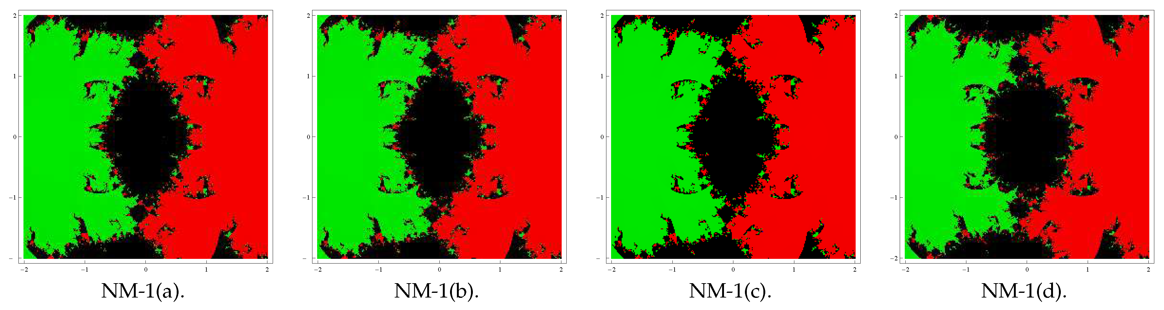
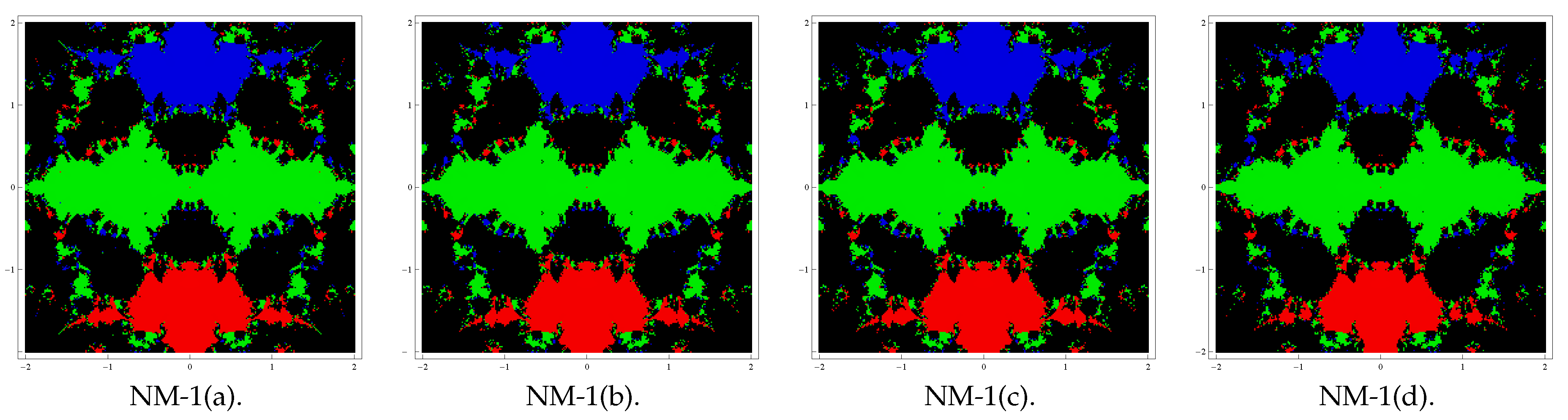
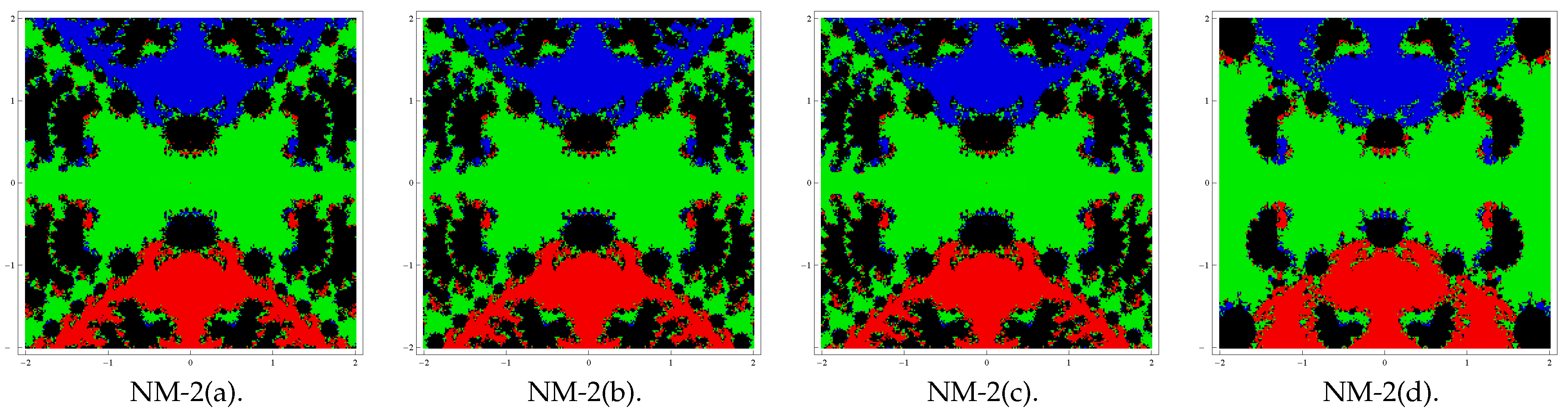
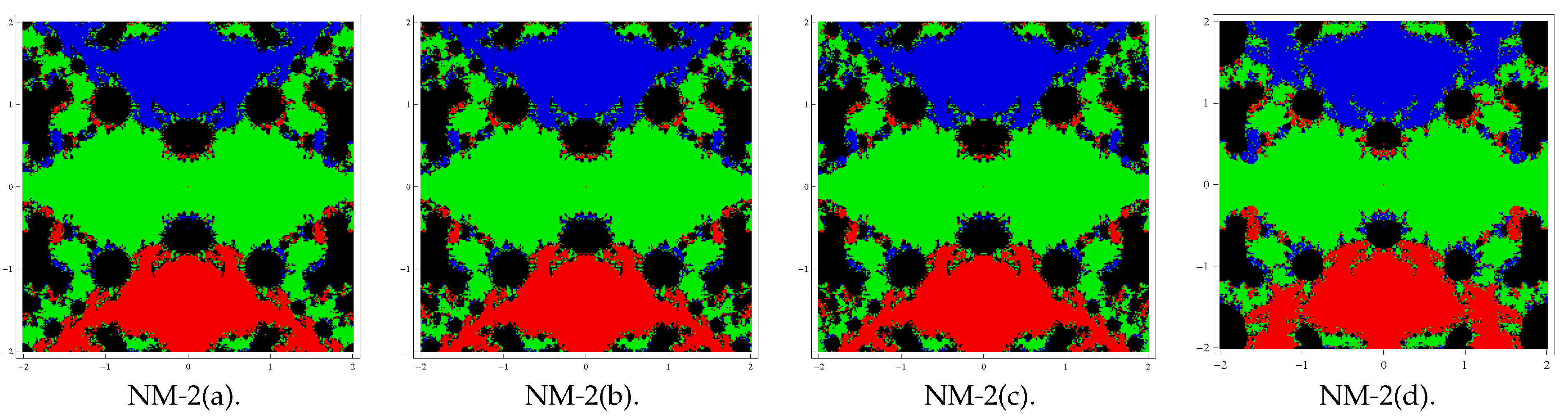
Here, our aim is to analyze the complex dynamics of the proposed methods based on the visual display of the basins of attraction of the zeros of a polynomial in the complex plane. Analysis of the complex dynamical behavior gives important information about the convergence and stability of an iterative scheme. Initially, Vrscay and Gilbert [23] introduced the idea of analyzing complex dynamics. Later on, many researchers used this concept in their work, for example (see [24,25,26] and the references therein). We choose some of the special cases (corresponding to the above forms of and ) of family (4) to analyze the basins. Let us choose the combinations of special Cases II(c) (for ) and II(d) with I(a), I(b), I(c), and I(d) in (4) and denote the corresponding new methods by NM-i(j), i = 1, 2 and j = a, b, c, d.
We take the initial point as , where D is a rectangular region in containing all the roots of The iterative methods starting at a point in a rectangle either converge to the zero of the function or eventually diverge. The stopping criterion considered for convergence is up to a maximum of 25 iterations. If the desired tolerance is not achieved in 25 iterations, we do not continue and declare that the iterative method starting at point does not converge to any root. The strategy adopted is the following: A color is assigned to each starting point in the basin of attraction of a zero. If the iteration starting from the initial point converges, then it represents the basins of attraction with that particular color assigned to it, and if it fails to converge in 25 iterations, then it shows the black color.
To view complex geometry, we analyze the attraction basins for the methods NM-1(a–d) and NM-2(a–d) on the following two polynomials:
Problem 1.
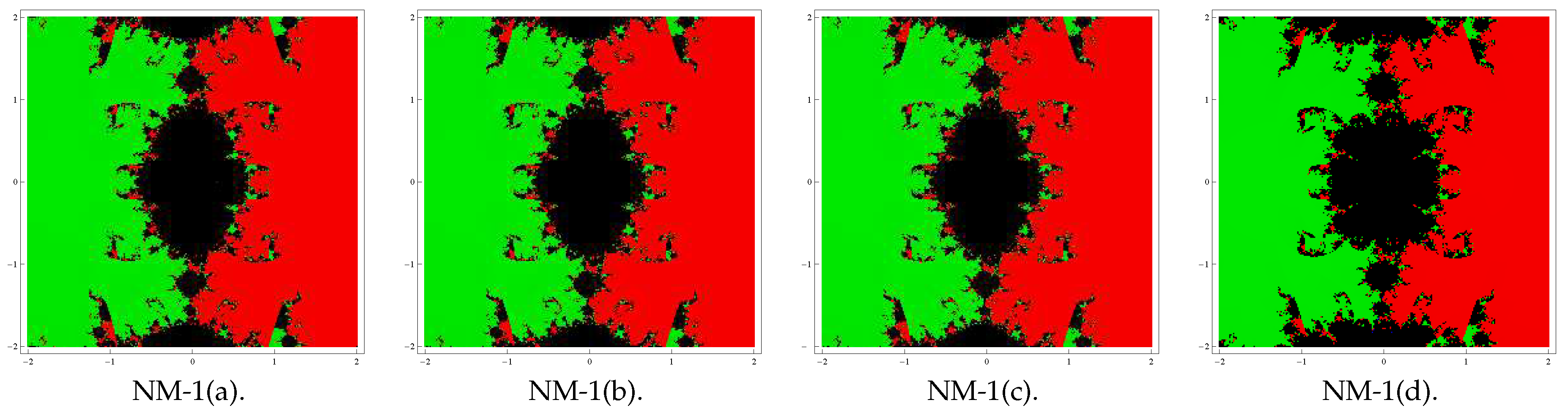
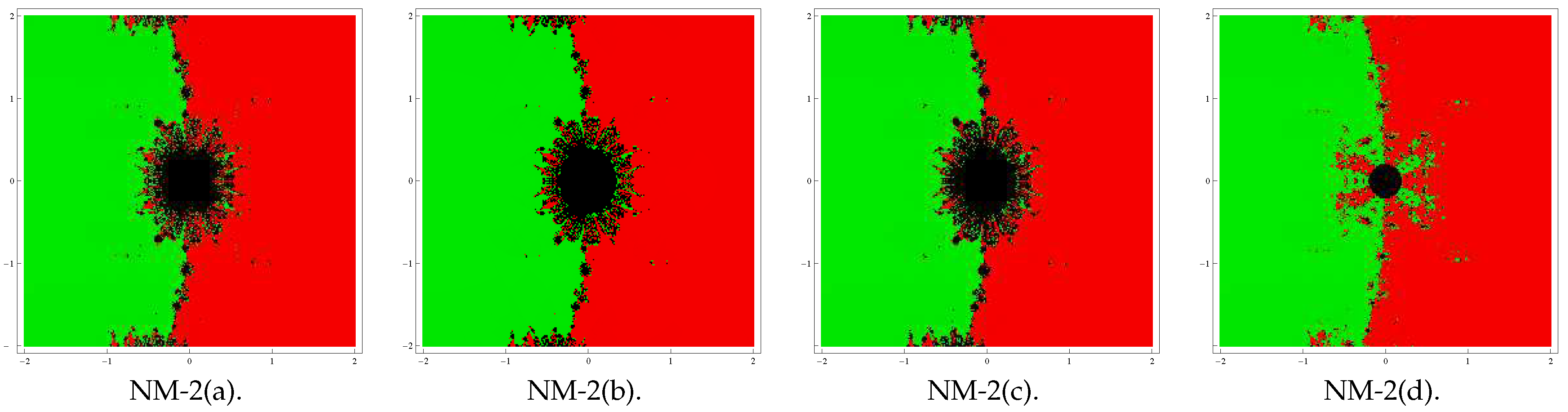
In the first example, we consider the polynomial , which has zeros with multiplicity two. In this case, we use a grid of points in a rectangle of size and assign the color green to each initial point in the basin of attraction of zero ‘’ and the color red to each point in the basin of attraction of zero ‘’. Basins obtained for the methods NM-1(a–d) and NM-2(a–d) are shown in Figure 1, Figure 2, Figure 3 and Figure 4 corresponding to . Observing the behavior of the methods, we see that the method NM-2(d) possesses a lesser number of divergent points and therefore has better stability than the remaining methods. Notice that there is a small difference in the basins for the rest of the methods with the same value of β. Notice also that the basins are becoming wider as parameter β assumes smaller values.
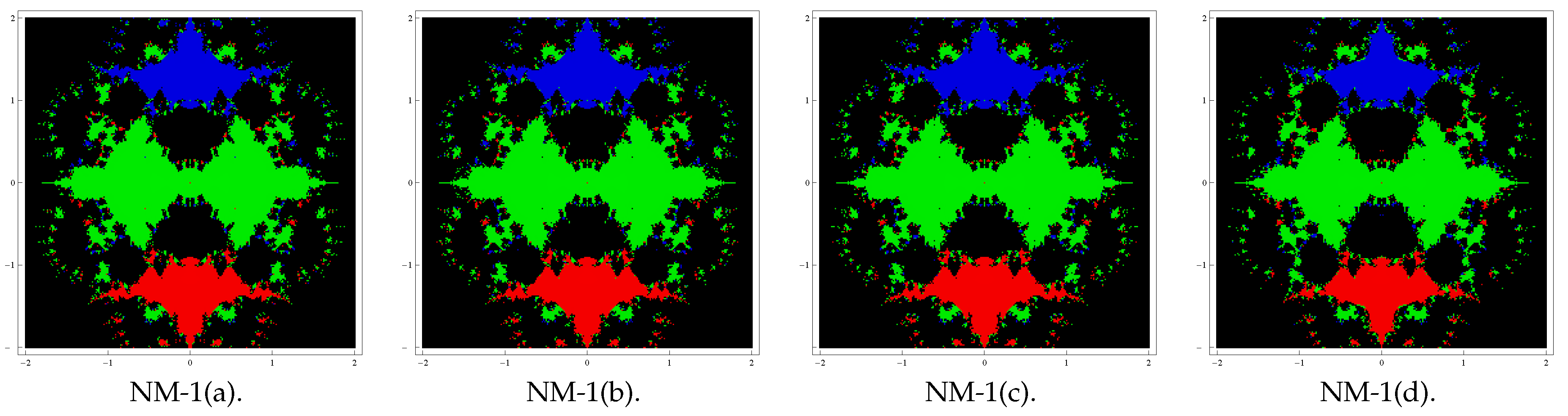
Problem 2.
Let us take the polynomial having zeros with multiplicity three. To see the dynamical view, we consider a rectangle with grid points and allocate the colors red, green, and blue to each point in the basin of attraction of , 0, and i, respectively. Basins for this problem are shown in Figure 5, Figure 6, Figure 7 and Figure 8 corresponding to parameter choices in the proposed methods. Observing the behavior, we see that again, the method NM-2(d) has better convergence behavior due to a lesser number of divergent points. Furthermore, observe that in each case, the basins are becoming larger with the smaller values of β. The basins in the remaining methods other than NM-2(d) are almost the same.
From the graphics, we can easily observe the behavior and applicability of any method. If we choose an initial guess in a region wherein different basins of attraction touch each other, it is difficult to predict which root is going to be attained by the iterative method that starts from . Therefore, the choice of in such a region is not a good one. Both black regions and the regions with different colors are not suitable to assume the initial guess as when we are required to achieve a particular root. The most intricate geometry is between the basins of attraction, and this corresponds to the cases where the method is more demanding with respect to the initial point. We conclude this section with a remark that the convergence behavior of the proposed techniques depends on the value of parameter . The smaller the value of is, the better the convergence of the method.
4. Numerical Examples and Discussion
In this section, we implement the special cases NM-1(a–d) and NM-2(a–d) that we have considered in the previous section of the family (4), to obtain zeros of nonlinear functions. This will not only illustrate the methods’ practically, but also serve to test the validity of theoretical results. The theoretical order of convergence is also confirmed by calculating the computational order of convergence (COC) using the formula (see [27]):
The performance is compared with some well-known higher order multiple-root solvers such as the sixth order methods by Geum et al. [8,9], which are expressed below:
First method by Geum et al. [8]:
where and , and is a holomorphic function in the neighborhood of origin (0, 0). The authors have also studied various forms of the function leading to sixth order convergence of (21). We consider the following four special cases of function in the formula (21) and denote the corresponding methods by GKN-1(j), j = a, b, c, d:
- (a)
- (b)
- (c)
- where , , , and
- (d)
- where , ,, and .
Second method by Geum et al. [9]:
where and . The function is analytic in a neighborhood of 0, and is holomorphic in a neighborhood of . Numerous cases of and have been proposed in [9]. We consider the following four special cases and denote the corresponding methods by GKN-2(j), j = a, b, c, d:
- (a)
- ,
- (b)
- ,
- (c)
- ,
- (d)
- ,
Computations were carried out in the programming package Mathematica with multiple-precision arithmetic. Numerical results shown in Table 1, Table 2, Table 3 and Table 4 include: (i) the number of iterations required to converge to the solution, (ii) the values of the last three consecutive errors , (iii) the computational order of convergence (COC), and (iv) the elapsed CPU time (CPU-time). The necessary iteration number and elapsed CPU time are calculated by considering as the stopping criterion.
The convergence behavior of the family of iterative methods (4) is tested on the following problems:
Example 1.
(Eigenvalue problem). Finding eigenvalues of a large square matrix is one of the difficult tasks in applied mathematics and engineering. Finding even the roots of the characteristic equation of a square matrix of order greater than four is a big challenge. Here, we consider the following 6 × 6 matrix:
The characteristic equation of the above matrix is given as follows:
This function has one multiple zero at of multiplicity three. We choose initial approximation . Numerical results are shown in Table 1.
Example 2.
(Kepler’s equation). Let us consider Kepler’s equation:
A numerical study, for different values of the parameters α and K, has been performed in [28]. As a particular example, let us take and . Consider this particular case four times with same values of the parameters, then the required nonlinear function is:
This function has one multiple zero at of multiplicity four. The required zero is calculated using initial approximation . Numerical results are displayed in Table 2.
Example 3.
(Manning’s equation). Consider the isentropic supersonic flow around a sharp expansion corner. The relationship between the Mach number before the corner (i.e., ) and after the corner (i.e., ) is given by (see [3]):
where and γ is the specific heat ratio of the gas.
As a particular case study, the equation is solved for given that , , and . Then, we have that:
where .
Consider this particular case three times with the same values of the parameters, then the required nonlinear function is:
This function has one multiple zero at of multiplicity three. The required zero is calculated using initial approximation . Numerical results are shown in Table 3.
Example 4.
Next, consider the standard nonlinear test function:
which has a multiple zero at of multiplicity four. Numerical results are shown in Table 4 with initial guess .
Example 5.
Consider the standard function, which is given as (see [8]):
The multiple zero of function is with multiplicity five. We choose the initial approximation for obtaining the zero of the function. Numerical results are exhibited in Table 5.
Example 6.
Consider another standard function, which is given as:
which has a zero of multiplicity three. Let us choose the initial approximation for obtaining the zero of the function. Numerical results are shown in Table 6.
Example 7.
Finally, considering yet another standard function:
The zero of function is with multiplicity four. We choose the initial approximation to find the zero of this function. Numerical results are displayed in Table 7.
It is clear from the numerical results shown in Table 1, Table 2, Table 3, Table 4, Table 5, Table 6 and Table 7 that the accuracy in the successive approximations increases as the iterations proceed. This shows the stable nature of the methods. Moreover, the present methods like that of existing methods show consistent convergence behavior. We display the value zero of in the iteration at which . The values of the computational order of convergence exhibited in the penultimate column in each table verify the theoretical order of convergence. However, this is not true for the existing methods GKN-1(a–d) and GKN-2(a) in Example 2. The entries in the last column in each table show that the new methods use less computing time than the time used by existing methods. This verifies the computationally-efficient nature of the new methods. Similar numerical tests, performed for many problems of different types, have confirmed the aforementioned conclusions to a large extent.
We conclude the analysis with an important problem regarding the choice of initial approximation in the practical application of iterative methods. The required convergence speed of iterative methods can be achieved in practice if the selected initial approximation is sufficiently close to the root. Therefore, when applying the methods for solving nonlinear equations, special care must be given for guessing close initial approximations. Recently, an efficient procedure for obtaining sufficiently close initial approximation has been proposed in [29]. For example, the procedure when applied to the function of Example 1 in the interval [0, 1.5] using the statements:
in programming package Mathematica yields a close initial approximation to the root .
f[x_ ]=x^6-12x^5+56x^4-130x^3+159x^2-98x+24; a=0; b=1.5;
k=1; x0=0.5∗(a+b+Sign[f[a]]∗NIntegrate[Tanh[k∗f[x]],{x,a,b}])
k=1; x0=0.5∗(a+b+Sign[f[a]]∗NIntegrate[Tanh[k∗f[x]],{x,a,b}])
5. Conclusions
In the present work, we have designed a class of seventh order derivative-free iterative techniques for computing multiple zeros of nonlinear functions, with known multiplicity. The analysis of convergence shows the seventh order convergence under standard assumptions for the nonlinear function, the zeros of which we have searched. Some special cases of the class were stated. They were applied to solve some nonlinear equations and also compared with existing techniques. Comparison of the numerical results showed that the presented derivative-free methods are good competitors of the existing sixth order techniques that require derivative evaluations. The paper is concluded with the remark that unlike the methods with derivatives, the methods without derivatives are rare in the literature. Moreover, such algorithms are good options to Newton-like iterations in the situation when derivatives are difficult to compute or expensive to obtain.
Author Contributions
Methodology, J.R.S.; writing, review and editing, J.R.S.; investigation, D.K.; data curation, D.K.; conceptualization, I.K.A.; formal analysis, I.K.A.
Funding
This research received no external funding.
Conflicts of Interest
The authors declare no conflict of interest.
References
- Argyros, I.K. Convergence and Applications of Newton-Type Iterations; Springer: New York, NY, USA, 2008. [Google Scholar]
- Argyros, I.K.; Magreñán, Á.A. Iterative Methods and Their Dynamics with Applications; CRC Press: New York, NY, USA, 2017. [Google Scholar]
- Hoffman, J.D. Numerical Methods for Engineers and Scientists; McGraw-Hill Book Company: New York, NY, USA, 1992. [Google Scholar]
- Schröder, E. Über unendlich viele Algorithmen zur Auflösung der Gleichungen. Math. Ann. 1870, 2, 317–365. [Google Scholar] [CrossRef]
- Hansen, E.; Patrick, M. A family of root finding methods. Numer. Math. 1977, 27, 257–269. [Google Scholar] [CrossRef]
- Behl, R.; Cordero, A.; Motsa, S.S.; Torregrosa, J.R. On developing fourth-order optimal families of methods for multiple roots and their dynamics. Appl. Math. Comput. 2015, 265, 520–532. [Google Scholar] [CrossRef]
- Behl, R.; Cordero, A.; Motsa, S.S.; Torregrosa, J.R.; Kanwar, V. An optimal fourth-order family of methods for multiple roots and its dynamics. Numer. Algorithms 2016, 71, 775–796. [Google Scholar] [CrossRef]
- Geum, Y.H.; Kim, Y.I.; Neta, B. A class of two-point sixth-order multiple-zero finders of modified double-Newton type and their dynamics. Appl. Math. Comput. 2015, 270, 387–400. [Google Scholar] [CrossRef]
- Geum, Y.H.; Kim, Y.I.; Neta, B. A sixth–order family of three–point modified Newton–like multiple–root finders and the dynamics behind their extraneous fixed points. Appl. Math. Comput. 2016, 283, 120–140. [Google Scholar] [CrossRef]
- Li, S.G.; Cheng, L.Z.; Neta, B. Some fourth-order nonlinear solvers with closed formulae for multiple roots. Comput. Math. Appl. 2010, 59, 126–135. [Google Scholar] [CrossRef]
- Li, S.; Liao, X.; Cheng, L. A new fourth-order iterative method for finding multiple roots of nonlinear equations. Appl. Math. Comput. 2009, 215, 1288–1292. [Google Scholar]
- Liu, B.; Zhou, X. A new family of fourth-order methods for multiple roots of nonlinear equations. Nonlinear Anal. Model. Control 2013, 18, 143–152. [Google Scholar]
- Neta, B. Extension of Murakami’s high-order nonlinear solver to multiple roots. Int. J. Comput. Math. 2010, 87, 1023–1031. [Google Scholar] [CrossRef]
- Sharifi, M.; Babajee, D.K.R.; Soleymani, F. Finding the solution of nonlinear equations by a class of optimal methods. Comput. Math. Appl. 2012, 63, 764–774. [Google Scholar] [CrossRef]
- Sharma, J.R.; Sharma, R. Modified Jarratt method for computing multiple roots. Appl. Math. Comput. 2010, 217, 878–881. [Google Scholar] [CrossRef]
- Soleymani, F.; Babajee, D.K.R. Computing multiple zeros using a class of quartically convergent methods. Alex. Eng. J. 2013, 52, 531–541. [Google Scholar] [CrossRef]
- Soleymani, F.; Babajee, D.K.R.; Lotfi, T. On a numerical technique for finding multiple zeros and its dynamics. J. Egypt. Math. Soc. 2013, 21, 346–353. [Google Scholar] [CrossRef]
- Victory, H.D.; Neta, B. A higher order method for multiple zeros of nonlinear functions. Int. J. Comput. Math. 1983, 12, 329–335. [Google Scholar] [CrossRef]
- Zhou, X.; Chen, X.; Song, Y. Constructing higher-order methods for obtaining the multiple roots of nonlinear equations. J. Comput. Math. Appl. 2011, 235, 4199–4206. [Google Scholar] [CrossRef]
- Zhou, X.; Chen, X.; Song, Y. Families of third and fourth order methods for multiple roots of nonlinear equations. Appl. Math. Comput. 2013, 219, 6030–6038. [Google Scholar] [CrossRef]
- Osada, N. An optimal multiple root-finding method of order three. J. Comput. Appl. Math. 1994, 51, 131–133. [Google Scholar] [CrossRef]
- Traub, J.F. Iterative Methods for the Solution of Equations; Chelsea Publishing Company: New York, NY, USA, 1982. [Google Scholar]
- Vrscay, E.R.; Gilbert, W.J. Extraneous fixed points, basin boundaries and chaotic dynamics for Schröder and König rational iteration functions. Numer. Math. 1988, 52, 1–16. [Google Scholar] [CrossRef]
- Varona, J.L. Graphic and numerical comparison between iterative methods. Math. Intell. 2002, 24, 37–46. [Google Scholar] [CrossRef]
- Scott, M.; Neta, B.; Chun, C. Basin attractors for various methods. Appl. Math. Comput. 2011, 218, 2584–2599. [Google Scholar] [CrossRef]
- Lotfi, T.; Sharifi, S.; Salimi, M.; Siegmund, S. A new class of three-point methods with optimal convergence order eight and its dynamics. Numer. Algorithms 2015, 68, 261–288. [Google Scholar] [CrossRef]
- Weerakoon, S.; Fernando, T.G.I. A variant of Newton’s method with accelerated third-order convergence. Appl. Math. Lett. 2000, 13, 87–93. [Google Scholar] [CrossRef]
- Danby, J.M.A.; Burkardt, T.M. The solution of Kepler’s equation. I. Celest. Mech. 1983, 40, 95–107. [Google Scholar] [CrossRef]
- Yun, B.I. A non-iterative method for solving non-linear equations. Appl. Math. Comput. 2008, 198, 691–699. [Google Scholar] [CrossRef]
Figure 1.
Basins of attraction for NM-1 (for ) in polynomial .

Figure 2.
Basins of attraction for NM-1 (for ) in polynomial .

Figure 3.
Basins of attraction for NM-2 (for ) in polynomial .

Figure 4.
Basins of attraction for NM-2 (for ) in polynomial .

Figure 5.
Basins of attraction for NM-1 (for ) in polynomial .

Figure 6.
Basins of attraction for NM-1 (for ) in polynomial .

Figure 7.
Basins of attraction for NM-2 (for ) in polynomial .

Figure 8.
Basins of attraction for NM-2 (for ) in polynomial .


Table 1.
Comparison of the performance of methods for Example 1.
| Methods | n | COC | CPU-Time | |||
|---|---|---|---|---|---|---|
| GKN-1(a) | 4 | 6.0000 | 0.05475 | |||
| GKN-1(b) | 4 | 6.0000 | 0.05670 | |||
| GKN-1(c) | 4 | 6.0000 | 0.05856 | |||
| GKN-1(d) | 4 | 6.0000 | 0.05504 | |||
| GKN-2(a) | 4 | 6.0000 | 0.07025 | |||
| GKN-2(b) | 4 | 6.0000 | 0.05854 | |||
| GKN-2(c) | 4 | 6.0000 | 0.06257 | |||
| GKN-2(d) | 5 | 6.0000 | 0.07425 | |||
| NM-1(a) | 4 | 7.0000 | 0.04675 | |||
| NM-1(b) | 4 | 6.9990 | 0.05073 | |||
| NM-1(c) | 4 | 6.9998 | 0.05355 | |||
| NM-1(d) | 4 | 6.9990 | 0.05077 | |||
| NM-2(a) | 4 | 6.9997 | 0.05435 | |||
| NM-2(b) | 4 | 6.9998 | 0.05454 | |||
| NM-2(c) | 4 | 6.9996 | 0.05750 | |||
| NM-2(d) | 4 | 6.9998 | 0.05175 |
Table 2.
Comparison of the performance of methods for Example 2.
| Methods | n | COC | CPU-Time | |||
|---|---|---|---|---|---|---|
| GKN-1(a) | 5 | 3.0018 | 2.1405 | |||
| GKN-1(b) | 5 | 3.0018 | 2.1445 | |||
| GKN-1(c) | 5 | 3.0018 | 2.1835 | |||
| GKN-1(d) | 5 | 3.0018 | 2.1797 | |||
| GKN-2(a) | 5 | 1.1923 | 1.8047 | |||
| GKN-2(b) | 4 | 6.0000 | 1.4452 | |||
| GKN-2(c) | 4 | 6.0000 | 1.4415 | |||
| GKN-2(d) | 4 | 6.0000 | 1.4492 | |||
| NM-1(a) | 3 | 7.0000 | 0.9845 | |||
| NM-1(b) | 3 | 7.0000 | 0.9650 | |||
| NM-1(c) | 3 | 7.0000 | 0.9570 | |||
| NM-1(d) | 3 | 7.0540 | 0.8590 | |||
| NM-2(a) | 3 | 7.0000 | 0.9842 | |||
| NM-2(b) | 3 | 7.0000 | 0.9607 | |||
| NM-2(c) | 3 | 7.0000 | 0.9767 | |||
| NM-2(d) | 3 | 7.0540 | 0.7460 |
Table 3.
Comparison of the performance of methods for Example 3.
| Methods | n | COC | CPU-Time | |||
|---|---|---|---|---|---|---|
| GKN-1(a) | 4 | 6.0000 | 1.3047 | |||
| GKN-1(b) | 4 | 6.0000 | 1.2852 | |||
| GKN-1(c) | 4 | 6.0000 | 1.3203 | |||
| GKN-1(d) | 4 | 6.0000 | 1.2970 | |||
| GKN-2(a) | 4 | 6.0000 | 1.2382 | |||
| GKN-2(b) | 4 | 6.0000 | 1.2440 | |||
| GKN-2(c) | 4 | 6.0000 | 1.2422 | |||
| GKN-2(d) | 4 | 6.0000 | 1.2577 | |||
| NM-1(a) | 4 | 0 | 7.0000 | 1.0274 | ||
| NM-1(b) | 4 | 0 | 7.0000 | 1.0272 | ||
| NM-1(c) | 4 | 0 | 7.0000 | 1.0231 | ||
| NM-1(d) | 4 | 0 | 7.0000 | 1.0235 | ||
| NM-2(a) | 4 | 0 | 7.0000 | 1.0398 | ||
| NM-2(b) | 4 | 0 | 7.0000 | 1.0742 | ||
| NM-2(c) | 4 | 0 | 7.0000 | 1.0467 | ||
| NM-2(d) | 4 | 0 | 7.0000 | 1.0192 |
Table 4.
Comparison of the performance of methods for Example 4.
| Methods | n | COC | CPU-Time | |||
|---|---|---|---|---|---|---|
| GKN-1(a) | 4 | 6.0000 | 0.1017 | |||
| GKN-1(b) | 4 | 5.9999 | 0.0977 | |||
| GKN-1(c) | 4 | 5.9999 | 0.1055 | |||
| GKN-1(d) | 4 | 5.9999 | 0.1015 | |||
| GKN-2(a) | 4 | 5.9999 | 0.1132 | |||
| GKN-2(b) | 4 | 5.9999 | 0.1052 | |||
| GKN-2(c) | 4 | 5.9999 | 0.1055 | |||
| GKN-2(d) | 4 | 5.9999 | 0.1095 | |||
| NM-1(a) | 4 | 6.9999 | 0.0720 | |||
| NM-1(b) | 4 | 6.9999 | 0.0724 | |||
| NM-1(c) | 4 | 6.9999 | 0.0722 | |||
| NM-1(d) | 4 | 6.9999 | 0.0782 | |||
| NM-2(a) | 4 | 6.9999 | 0.0732 | |||
| NM-2(b) | 4 | 6.9999 | 0.0723 | |||
| NM-2(c) | 4 | 6.9999 | 0.0746 | |||
| NM-2(d) | 4 | 6.9999 | 0.0782 |
Table 5.
Comparison of the performance of methods for Example 5.
| Methods | n | COC | CPU-Time | |||
|---|---|---|---|---|---|---|
| GKN-1(a) | 4 | 6.0000 | 0.5820 | |||
| GKN-1(b) | 4 | 6.0000 | 0.5860 | |||
| GKN-1(c) | 4 | 6.0000 | 0.5937 | |||
| GKN-1(d) | 4 | 6.0000 | 0.5832 | |||
| GKN-2(a) | 4 | 6.0000 | 0.7120 | |||
| GKN-2(b) | 4 | 6.0000 | 0.6992 | |||
| GKN-2(c) | 4 | 6.0000 | 0.6915 | |||
| GKN-2(d) | 4 | 6.0000 | 0.6934 | |||
| NM-1(a) | 4 | 7.0000 | 0.3712 | |||
| NM-1(b) | 4 | 7.0000 | 0.3360 | |||
| NM-1(c) | 4 | 7.0000 | 0.3555 | |||
| NM-1(d) | 4 | 7.0000 | 0.3633 | |||
| NM-2(a) | 4 | 7.0000 | 0.3585 | |||
| NM-2(b) | 4 | 7.0000 | 0.3592 | |||
| NM-2(c) | 4 | 7.0000 | 0.3791 | |||
| NM-2(d) | 4 | 7.0000 | 0.3467 |
Table 6.
Comparison of the performance of methods for Example 6.
| Methods | n | COC | CPU-Time | |||
|---|---|---|---|---|---|---|
| GKN-1(a) | 4 | 6.0000 | 3.8670 | |||
| GKN-1(b) | 4 | 6.0000 | 4.1287 | |||
| GKN-1(c) | 4 | 5.9999 | 3.8866 | |||
| GKN-1(d) | 4 | 6.0000 | 4.5195 | |||
| GKN-2(a) | 5 | 5.4576 | 5.5310 | |||
| GKN-2(b) | 4 | 6.0000 | 3.9647 | |||
| GKN-2(c) | 4 | 5.9995 | 3.7772 | |||
| GKN-2(d) | 8 | 6.0000 | 6.2194 | |||
| NM-1(a) | 4 | 7.0000 | 1.9372 | |||
| NM-1(b) | 4 | 7.0000 | 1.5625 | |||
| NM-1(c) | 4 | 7.0000 | 1.5662 | |||
| NM-1(d) | 4 | 7.0000 | 1.5788 | |||
| NM-2(a) | 4 | 7.0000 | 1.5900 | |||
| NM-2(b) | 4 | 7.0000 | 1.5585 | |||
| NM-2(c) | 4 | 7.0000 | 1.6405 | |||
| NM-2(d) | 4 | 7.0000 | 1.3444 |
Table 7.
Comparison of the performance of methods for Example 7.
| Methods | n | COC | CPU-Time | |||
|---|---|---|---|---|---|---|
| GKN-1(a) | 4 | 6.0000 | 1.7305 | |||
| GKN-1(b) | 4 | 6.0000 | 1.7545 | |||
| GKN-1(c) | 4 | 6.0000 | 1.7150 | |||
| GKN-1(d) | 4 | 6.0000 | 1.7852 | |||
| GKN-2(a) | 4 | 6.0000 | 1.6405 | |||
| GKN-2(b) | 4 | 6.0000 | 1.7813 | |||
| GKN-2(c) | 4 | 6.0000 | 1.7382 | |||
| GKN-2(d) | 4 | 6.0000 | 1.9150 | |||
| NM-1(a) | 4 | 7.0000 | 1.0077 | |||
| NM-1(b) | 4 | 7.0000 | 0.9062 | |||
| NM-1(c) | 4 | 7.0000 | 1.0040 | |||
| NM-1(d) | 4 | 7.0000 | 1.0054 | |||
| NM-2(a) | 4 | 7.0000 | 0.8867 | |||
| NM-2(b) | 4 | 7.0000 | 0.9802 | |||
| NM-2(c) | 4 | 7.0000 | 0.9412 | |||
| NM-2(d) | 4 | 7.0000 | 0.9142 |
© 2019 by the authors. Licensee MDPI, Basel, Switzerland. This article is an open access article distributed under the terms and conditions of the Creative Commons Attribution (CC BY) license (http://creativecommons.org/licenses/by/4.0/).
Share and Cite
MDPI and ACS Style
Sharma, J.R.; Kumar, D.; Argyros, I.K. An Efficient Class of Traub-Steffensen-Like Seventh Order Multiple-Root Solvers with Applications. Symmetry 2019, 11, 518. https://doi.org/10.3390/sym11040518
AMA Style
Sharma JR, Kumar D, Argyros IK. An Efficient Class of Traub-Steffensen-Like Seventh Order Multiple-Root Solvers with Applications. Symmetry. 2019; 11(4):518. https://doi.org/10.3390/sym11040518
Chicago/Turabian StyleSharma, Janak Raj, Deepak Kumar, and Ioannis K. Argyros. 2019. "An Efficient Class of Traub-Steffensen-Like Seventh Order Multiple-Root Solvers with Applications" Symmetry 11, no. 4: 518. https://doi.org/10.3390/sym11040518
Note that from the first issue of 2016, this journal uses article numbers instead of page numbers. See further details here.