Has Land Finance Increased Local Financial Risks in China?

Abstract

Whether land finance has increased local financial risks has always been a hot topic in society and in the academic circle. This article firstly describes the overall characteristics of the development of local finance in China. By establishing a matrix containing 16 indicators for local financial risks, it has analyzed the characteristics and overall development trend of financial risks at the provincial level in China as a whole. Furthermore, it explores the casual effect of land finance on local financial risks by ordinary least squares (OLS) and two-stage least squares (2SLS) models on the basis of panel data covering 178 prefecture-level cities from 2009 to 2017. The results show that from 2017 to 2019, there still existed great risks in local finance in all provinces and cities across the country, and the local financial risks of all provinces and cities showed an upward trend and were mostly related to the high dependence on land finance. By analyzing the data of the last decade, we can find that the government’s dependence on land finance had increased, along with the increasing financial risks which it faced. In particular, they exerted a more prominent impact on the eastern regions and other regions with a low urbanization rate in China.

1. Introduction

Land finance is an important part of local finance in China as well as a financial operation mode for obtaining income from land resources. We found that the systematic analysis about the causes and risks of Land Finance was firstly published by Jiang and Liu [1], members of the Land Research Group of the Development Research Center of the State Council in 2006. Since the 21st Century, with the rapid development of China’s economy, the cities and constantly emerging urban agglomerations in China have brought about dual effects in both space and scale. They played a leading role in promoting China’s economic take-off and creating a large amount of “urban wealth”. The key system for the implementation of urbanization in China is just land finance, which contributed to the primitive accumulation of capital urgently needed in China’s urban development [2]. In particular, since the system of “tendering, auction and offering” was introduced in China in 2002, there has been a trend of rapid expansion in the scale of land finance. In 2019, the land-transferring fees registered USD 1.01 trillion, accounting for 69.88% of the total local fiscal revenue and 7.13% of the GDP of China. The data of land-transferring fees are obtained from iFinD database. In 2019, the income from the transfers of state-owned land use rights registered USD 101.306 billion; the data of local fiscal revenue and national GDP come from the data released by the National Bureau of Statistics. In 2019, the local fiscal revenue was USD 1448.935 billion, and the GDP in 2019 was USD 14,203.508 billion. Under the background of full implementation of the tax distribution system reform, there occurred increasing competition among local governments for capital, as well as the obvious dislocation with respect to administrative power and financial power. On the one hand, this created favorable conditions for the development of the secondary industry and tertiary industry; on the other hand, however, the dependence of local governments on land finance was further intensified, thus causing a negative impact on the rationality of local finance. For local governments, under the influence of market economy, the current land transfer mechanism has led to a substantial increase in land prices. This has intensified the dependence of local governments on land finance at the institutional level. It should be emphasized that land finance is highly complex, involving various factors and closely related to the interests of all parties. In the overall process of industrialization and urbanization, land, as the core element, provided a huge space for revenue, and was operated and distributed among various subjects. The efficiency of economic system can be reflected in the operation of land finance [3].

The expansion of the proportion and scale of land finance is two-sided: on the one hand, it has increased the fiscal revenue of local governments and provided financial support for the development of local undertakings; on the other hand, with the increasing dependence of local governments on land finance, its financial risks are on the rise. Hence, the sustainability of this model has been widely questioned [4]. For local governments, both their own financial risks and bank liquidity risks have been greatly aggravated under the influence of the leverage of land finance, bringing hidden problems to the sustainable development of the local economy [5]. Under the background of macro-control, land-related revenue will continue decreasing, local governments will face more severe debt risks, the possibility of systemic risks in local finance will be greatly increased, and the financial risks and debt risks will reinforce each other [6]. In a word, the negative effects of land finance began to show up, the problem of asset bubble accumulation intensified, and the possibility of local government debt risks increased greatly. All of these posed a hidden danger for the outbreak of systemic financial risks [7].

From the 1990s, the academic circle began to study local financial risks, and comprehensively and systematically analyzed the influencing factors and causes of local financial risks. Research shows that local financial risks were closely related to the local financial structure. Once there arose any problem in the local financial structure, local financial risks would be aggravated to a great extent [8]. Under the tides of market economy, local financial risks had been aggravated to a large extent [9]. There existed hidden significant local financial risks for local governments in China due to huge debts in the form of contingent debts [10]. The unreasonable local fiscal expenditure structure will increase the dependence of local governments on extra-budgetary fiscal revenue and financing platforms, thus increasing local fiscal risks [11]. Scholars have also done much research on the measurement of local financial risks. Taking the public resources and the responsibilities for expenditure of local governments as the point of entry, this article constructs the corresponding mathematical analysis model, and measures the comprehensive indexes of land financial risks by combining with the AHP-entropy method, so as to scientifically and reasonably evaluate local financial risks [12].

The subsequent chapters of this paper are arranged as follows: Section 2 is about the overall measurement of local financial risks in China; Section 3 is about the measurement of the impact of land finance on local financial risks; and Section 4 is about the conclusion and policy recommendations.

2. The Overall Measurement of Local Financial Risks

2.1. General Characteristics of Local Finance in China

Since the reform and opening up was initiated, China’s economy has developed rapidly, and the autonomy of local governments has become more and more obvious. Local finance has played an increasingly important role in the national economic development, with the following potential concerns:

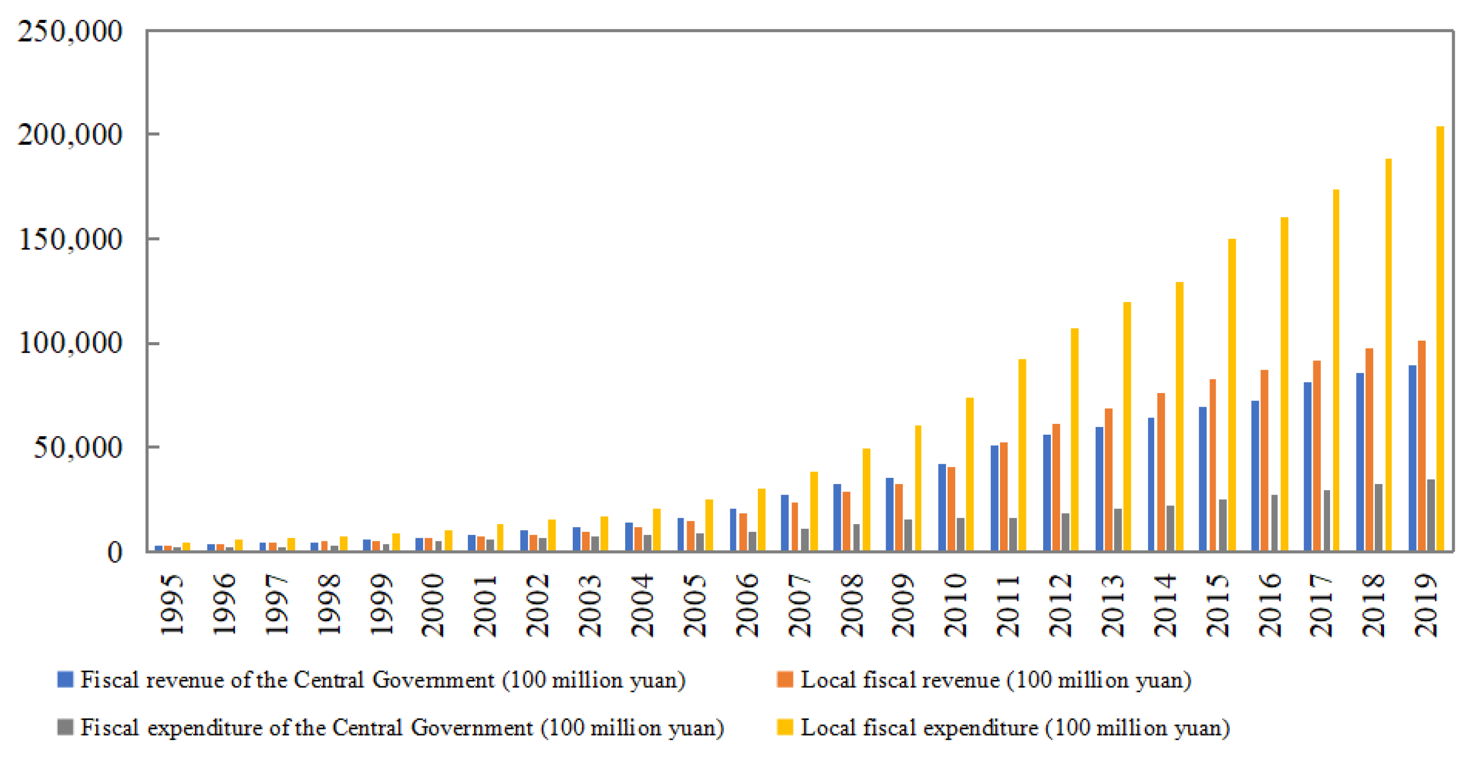
Firstly, the proportion of land revenue to local finance has been continuously increasing. From the development of fiscal revenue and expenditure of both the central and local governments in China over the past 25 years, we can see that the scale of local fiscal expenditure has been expanding greatly with soaring from USD 43 billion in 1995 to USD 1.4478 trillion in 2019, greatly exceeding that of central government. However, the central government expenditure was relatively stable, increasing from USD 28.793 billion in 1995 to USD 0.502 trillion in 2019, only an increase of 17.5 times. In 2019, the local financial expenditure was nearly six times the value of the central government financial expenditure. However, while local fiscal expenditure kept rising, the ratio of local fiscal revenue to central government fiscal revenue was stabilized at around 1:1. This difference between the fiscal revenue and the fiscal expenditure had brought great pressure upon local finance (as shown in Figure 1).

Second, local finance had lowered the national fiscal deficit ratio. From a national perspective, the reduction in the national fiscal deficit ratio could not be separated from the contribution of local fiscal revenue. In particular, since 2001, the national fiscal deficit ratio had dropped all the way from 2.27%; and in 2007, the national revenue and expenditure turned from losses into profits, while the deficit ratio was negative. With the increasing contribution of local finance to the national fiscal balance, the local fiscal deficit showed an upward trend, soaring from 3% in 1995 to over 10% in 2019. In this drastic change, the pressure of sustainable development of local finance increased.

Third, local governments were increasingly dependent on land finance for fiscal revenue. Under the background of full implementation of the tax distribution reform, local governments were faced with the separation of administrative and financial powers, while their financial pressure was on the increase. To a large extent, local governments were urged to take land resources as the main source of fiscal revenue, thus leading to its increasing dependence on land finance [13]. According to the local financial data of 2019, the income from local land transfers in China registered USD 0.9645 trillion, accounting for 66.4% of the local fiscal revenue, the highest over the past five years. Among the 31 provinces and cities, the ratio of land-transferring revenue to local fiscal revenue in 18 provinces and cities exceeded 50%, among which Hubei, Zhejiang, Anhui, JJiangsu and Fujian ranked among the top five, with the ratios of 128.9%, 128.4%, 97.0%, 96.2% and 93.0%, respectively. From the city level, the ratio of land-transferring revenue to local fiscal revenue in Wenzhou, Kunming, Fuzhou, Hangzhou, Taiyuan, Hefei, Wuhan, Guangzhou, Nanjing, Foshan and Zhengzhou exceeded 100%.

2.2. Overall Measurement of Local Financial Risks in China

The identification of local financial risks is complex and diverse, and a single index only cannot comprehensively, timely and accurately, reflect local financial risks and their development trends. In the research of local financial risks, prior research mainly uses “financial risk matrix”. According to the difference of risk exposure degree, local financial risks can be divided into four types: the first type is the direct explicit risk; the second type is the direct hidden risk; the third type is the contingent explicit risk; the fourth type is the contingent hidden risk. In other words, local financial risks cover two of the above four basic attributes; namely, direct and contingent, as well as implicit and explicit. Explicit risk refers to the specific local financial risk which is less difficult to confirm; its risk triggering factors are very obvious, and the risk losses can be accurately evaluated; implicit risk refers to the responsibility risk which local governments need to bear at the moral level, and common hidden risk includes the pressure from interested groups and the expectations of the public, while risk indicators are often difficult to effectively detect and their hidden state is relatively high; direct risk refers to the responsibilities which will arise under any circumstances, so they can be predicted according to some specific factors rather than determination; and contingent risk refers to the liabilities caused by any potential discontinuous events. Compared with other types of risks, the occurrence of contingent events is difficult to predict, and the losses caused thereby are often difficult to predict, too. At the same time, according to the iceberg theory of public debts [14], which is the expansion and supplement of Hana Polackova’s financial risk matrix by Liu, a famous financial expert in China in 2017, the debt on the top of the iceberg is certain, including direct explicit debt and contingent explicit debt, while the debt on the bottom of the iceberg is uncertain, including direct implicit debt and contingent implicit debt. That is to say, compared to the direct and explicit risks, the other three kinds of risks are relatively not transparent. Because of the concealment and incompleteness of their information, it is difficult for local governments to control them when they carry out macro-control, and they are more prone to “hit the rocks” and lead to systemic risks. The purpose of the iceberg theory is to reveal the uncertainty of government debt behavior and the difficulty in measuring public debt in the form of the bottom of the iceberg, so as to warn the government to pay more attention to the risk of public debt. Consequently, it is easy to cause systematic risks. Especially in China, on the basis of investigation and study, it has been concluded that the local financial risks in China are hidden and even deformed in the economic operation and are becoming increasingly complicated [15]. Therefore, it is of great significance to establish a comprehensive and effective early warning system for local financial risks so as to prevent any systemic risks.

2.2.1. Establishment of Local Financial Risk Matrixes

From the previous analysis, we can see that the overall risks of local finance are increasing under the background that China’s economy has entered a new normal. In order to measure the local financial risks in a more complete way, this article, based on the existing researches at home and abroad and combining with the development characteristics of local finance, the debt characteristics of local finance and the relationship between local finance and macro-economy in China, moreover, considering the comprehensiveness and representativeness of the fiscal revenue and expenditure, selected 16 evaluation indicators to form an early warning index system for local fiscal risks, which includes the direct explicit risk index (R${}_1$), contingent direct risk index (R${}_2$), direct implicit risk index (R${}_3$) or implicit risk index (R${}_4$). The selection of evaluation indicators includes not only the internationally-used measurement indicators as specified in the Maastricht Treaty such as debt burden ratio and fiscal deficit ratio, but also the economic growth rate and per capita disposable income growth rate that represent China’s macro-economic characteristics; moreover, it incorporates the evaluation indicators which reflect China’s financial characteristics, such as the annual financial distress coefficient and PPP investment scale of all provinces and cities which are released by the Ministry of Finance. For the setting of the risk thresholds of each evaluation indicator, we first refer to the values by the existing research and the authoritative institutions in China and other countries, and then refer to the characteristics of statistical values to set three risk zones of “mild early warning”, “intermediate early warning” and “serious early warning” for each evaluation indicator. Then, we sort and classify the financial risk indicators of all provinces and cities in China, and present the risk situation of local finance in China in recent years, so as to provide a basis for the empirical analysis of the impact of land finance on local financial risks in the next part.

Table 1. Indicators of the local financial risk matrixes.

Types of Financial Risks	Direct Risk	Contingent Risk
Explicit risk	R${}_1$ X${}_1$: Debt burden ratio = government debt balance/local GDP in the current year X${}_2$: Debt expenditure rate = new government debt/local public finance expenditure in the current year X${}_3$: Debt repayment rate = amount of repayment for principal and interest /total fiscal revenue in the current year X${}_4$: Financial distress coefficient uses the data published by the Ministry of Finance	R${}_2$ X${}_5$: Economic growth rate = local GDP growth X${}_6$: Growth rate of per capita disposable income of urban and rural residents, using the data from the National Bureau of Statistics X${}_7$: Unemployment rate = the number of unemployed people/total labor X${}_8$: Risk factor of financial balance = (the loan balance of financial departments−the deposit balance of financial departments)/fiscal revenue
Implicit risk	R${}_3$ X${}_9$: The elasticity of fiscal expenditure to fiscal revenue = the growth rate of fiscal expenditure/growth rate of fiscal revenue X${}_{10}$: Fiscal deficit ratio = fiscal deficit/local GDP X${}_{11}$: Fixed assets investment speed = fixed assets investment growth rate/local GDP growth X${}_{12}$: PPP investment scale = The total PPP investment/local GDP	R${}_4$ X${}_{13}$: Land financial dependence = Land financial revenue/financial revenue X${}_{14}$: Fiscal concentration = fiscal revenue/local GDP X${}_{15}$: The proportion of tax revenue in fiscal revenue = tax revenue/fiscal revenue X${}_{16}$: Local fiscal revenue and expenditure balance coefficient = (Local fiscal expenditure/national fiscal expenditure)/(Local fiscal revenue/National fiscal revenue)

explains the indicators selected for various kinds of risks in the local financial risk matrixes, while

Table 2. Statistical analysis of early warning indicators of financial risks in all provinces and cities from 2017 to 2019.

Name of Indicators		Mild Early Warning	Intermediate Early Warning	Serious Early Warning	Mean Value	Minimum Value	Maximum Value
R${}_1$	X${}_1$: Debt burden ratio	≤16%	16–25%	>25%	26.1%	7.5%	70.9%
	X${}_2$: Debt expenditure ratio	≤20%	20–40%	>40%	87.0%	13.8%	203.8%
	X${}_3$: Debt repayment ratio	≤15%	15–30%	>30%	16.2%	0.3%	61.8%
	X${}_4$: Financial distress coefficient	≤65.2%	65.2–82.8%	>82.8%	65.2%	20.0%	90.0%
R${}_2$	X${}_5$: Economic growth rate	6–12%	4–6% and 12–14%	<4% and >14%	6.8%	3.0%	10.2%
	X${}_6$: Growth rate of per capita disposable income of urban and rural residents	>7%	5–7%	<5%	8.0%	6.7%	13.3%
	X${}_7$: Unemployment rate	0–4.2%	4.2–7%	>7%	3.1%	1.4%	4.2%
	X${}_8$ Financial balance risk coefficient	>5%	2–5%	<2%	3.2%	−3.2%	16.2%
R${}_3$	X${}_9$: The elasticity of fiscal expenditure to fiscal revenue	<1.4	1.4–1.5	>1.5	1.6	−10.8	10.4
	X${}_{10}$: Fiscal deficit ratio	<3%	3–5%	>5%	−16.7%	−5.9%	114.1%
	X${}_{11}$: Speed of investment in fixed assets	>0.8	0.6–0.8	<0.6	0.70	−11.3	3.9
	X${}_{12}$: PPP investment scale	<10%	10–15%	>15%	17.4%	1.8%	73.0%
R${}_4$	X${}_{13}$: Land financial dependence	0–50%	50–100%	≥100%	58.0%	15.0%	128.9%
	X${}_{14}$: Fiscal concentration	25–30%	15–25%	0–15%	10.7%	5.5%	21.7%
	X${}_{15}$: The proportion of tax revenue in fiscal revenue	86–95%	77–86%	0–77%	74.4%	11.9%	122.7%
	X${}_{16}$: Coefficient of balance of local fiscal revenue and expenditure	0–1	1–1.5	>1.5	1.8	0.4	5.4

(Note: Tibet was not included in the calculation in X${}_2$, X${}_3$, X${}_{13}$, X${}_{14}$, X${}_{15}$, and X${}_{16}$ due to the lack of data. For the specific contents of the division of indexes of the local financial risk matrixes, please see the Appendix A to the paper).

gives a summary list of indicators for the local financial risk matrixes. Owing to space limitations, the specific explanations about 16 indicators are shown in the Appendix A.

The risk evaluation criteria of local financial risk matrixes are sorted according to the number of serious early warning indicators, the number of intermediate early warning indicators and the number of mild early warning indicators (

Table 3. The criteria for evaluating local financial risks.

Title Scenario Analysis	Low-Risk	Medium-Risk	High-Risk
Ordinary statistics method	≤4	4–9	≥9
Risk prudence principle method	≤4	4–7	≥7

). If the numbers of the above three indicators are the same, they will be sorted according to the numbers of direct explicit risks (R${}_1$), contingent explicit risks (R${}_2$), direct implicit risks (R${}_3$) and contingent implicit risks (R${}_4$). To make it convenient for the sorting, this paper sets the value of the serious early warning as 1, the intermediate early warning as 0.1 and the mild early warning as 0. The risk levels are divided in two ways (Table 3): one is the quartile analysis, in which the zone whose value is less than or equal to four is classified as the low-risk zone, the zone whose value is greater than four and less than nine is classified as the medium-risk zone, and the zone whose value is greater than or equal to nine is classified as the high-risk zone. The second is the risk prudence principle method. According to the quartile division method and the risk prudence method, the low-risk index value is retained, and the medium-risk index and high-risk index used as early warning are reduced by two; i.e., the zone with a value of less than or equal to four is classified as the low-risk zone, the zone with a value of greater than four and less than seven is classified as the medium-risk zone, and the zone with a value of greater than or equal to seven is classified as the high-risk zone.

2.2.2. Explanation of Data Collection

In this paper, a series of index data such as land transfer revenue, local GDP, local fiscal expenditure, national fiscal expenditure, national fiscal revenue and fiscal deficit ratio are obtained through iFinD, and relevant index data such as the per capita disposable income and the unemployment rate of urban and rural residents are obtained through the National Bureau of Statistics. Moreover, through the database of iFinD and in combination with those from the National Bureau of Statistics, we obtained such data as the investment speed of fixed assets, the ratio of the growth rate of fixed assets investment to the growth rate of local GDP, and the balance of local debts. Other data are as follows: the PPP investment scale comes from the national PPP comprehensive information platform, with the calculation method of the total PPP investment/local GDP. For new government debts, the data are from Wind Database, with the calculation method of the new local debts + city investment debt of each year. For the balance of government guaranteed debts, the indicators for the years of 2010, 2012 and June 2013 come from the indicators of guaranteed liability debt in the balance of local government debts at iFinD, while the data for other time periods are replaced by those of the existing local debts at iFinD. The annual amount of repayment of debts for both principal and interest come from the Wind Database, with the calculation method of the payment amount of local government debts + city investment debts. For the on-budget revenue of the current year, part of the data include the indicators of the total fiscal revenue in budget revenue at iFinD, and part of the data are obtained by summing up the on-budget revenue of all cities at CSMAR. For the total fiscal revenue, the data come from the total fiscal revenue of all provinces at iFinD, and the missed data of some provinces are supplemented by relevant data found on news reports. For the extra budgetary revenue, the data are obtained from iFinD, with the calculation method of the total fiscal revenue—the on-budget revenue.

Special Note: Due to the lack of some data of Tibet, the indicators of Tibet in X${}_2$, X${}_3$, X${}_{13}$, X${}_{14}$, X${}_{15}$, and X${}_{16}$ in the local financial risk system cannot be calculated, so Tibet has not been included in the ranking of 31 provinces and cities; however, Tibet was included in the overall national data, such as national GDP and national fiscal revenue and expenditure.

2.2.3. The Summary of Indicators

By adopting the matrix model of local financial risks and based on the collection and sorting of data, this paper obtained the results of the local financial risk matrixes of 31 provinces and cities in China in three recent years (2017–2019), which were summarized and analyzed. It is not easy to collect the local financial data before 2016, and there are not unified caliber and time of data release in different places. In 2016, when the 13th Five-year Plan was launched, the global economy was faced with a big downward pressure, while the transformation and upgrading of industries was in the ascendant and, under the background of increasing uncertainties, the Ministry of Finance fully implemented the basic requirement of seeking progress while maintaining stability, comprehensively promoted the development concept of the supply-side reform, and stimulated the total demand by virtue of the domestic market so as to achieve the stability and sustainability of the social and economic development. This paper holds that the relatively complete data from 2017 to 2019 and the results of local financial risk matrixes can reflect the current situation and development trend of local finance in China. It calculates and summarizes the local financial risk evaluation results of all provinces and cities over the past three years as

Table 4. The summary of the assessment results of financial risks of all provinces and cities from 2017 to 2019.

Province/City	2017 (1)	2018 (2)	2019 (3)	2017 (4)	2018 (5)	2019 (6)
Shanghai	★1.3	★1.4	★0.4	★1.3	★1.4	★0.4
Guangdong	★1.3	★1.3	★2.4	★1.3	★1.3	★2.4
Beijing	★1.5	★★4.4	★3.3	★1.5	★★4.4	★3.3
Shanxi	★3.2	★★7.3	★★7.3	★3.2	★★★7.3	★★★7.3
Jiangsu	★3.3	★3.5	★★4.4	★3.3	★3.5	★★4.4
Zhejiang	★3.5	★★5.4	★★6.4	★3.5	★★5.4	★★6.4
Shandong	★3.5	★3.7	★★6.6	★3.5	★3.7	★★6.6
Hebei	★★5.3	★★6.3	★★6.3	★★5.3	★★6.3	★★6.3
Henan	★★5.4	★★5.5	★★5.5	★★5.4	★★5.5	★★5.5
Hubei	★★5.4	★★7.3	★★6.5	★★5.4	★★★7.3	★★6.5
Hainan	★★5.4	★★6.6	★★7.4	★★5.4	★★6.6	★★★7.4
Shaanxi	★★5.4	★★6.5	★★★9.5	★★5.4	★★6.5	★★★9.5
Heilongjiang	★★5.5	★★6.5	★★6.3	★★5.5	★★6.5	★★6.3
Guangxi	★★5.5	★★8.3	★★7.4	★★5.5	★★★8.3	★★★7.4
Anhui	★★5.6	★★4.6	★★5.6	★★5.6	★★4.6	★★5.6
Fujian	★★6.2	★★5.3	★★4.4	★★6.2	★★5.3	★★4.4
Tianjin	★★6.3	★★5.6	★★7.4	★★6.3	★★5.6	★★★7.4
Chongqing	★★6.3	★★7.3	★★6.4	★★6.3	★★★7.3	★★6.4
Liaoning	★★6.4	★★5.6	★★7.4	★★6.4	★★5.6	★★★7.4
Jiangxi	★★6.4	★★7.4	★★7.5	★★6.4	★★★7.4	★★★7.5
Sichuan	★★6.5	★★5.5	★★6.5	★★6.5	★★5.5	★★6.5
Hunan	★★7.3	★★7.5	★★7.5	★★★7.3	★★★7.5	★★★7.5
Yunnan	★★7.3	★★7.2	★★8.3	★★★7.3	★★★7.2	★★★8.3
Xinjiang	★★7.3	★★★9.2	★★★9.3	★★★7.3	★★★9.2	★★★9.3
Jilin	★★7.4	★★7.5	★★★9.2	★★★7.4	★★★7.5	★★★9.2
Qinghai	★★8.1	★★★9.0	★★★9.1	★★★8.1	★★★9.0	★★★9.1
Inner Mongolia	★★8.3	★★8.3	★★6.4	★★★8.3	★★★8.3	★★6.4
Guizhou	★★8.3	★★8.2	★★★9.2	★★★8.3	★★★8.2	★★★9.2
Ningxia	★★★10.0	★★★9.1	★★★9.2	★★★10.0	★★★9.1	★★★9.2
Gansu	★★★11.1	★★★10.2	★★★10.2	★★★11.1	★★★10.2	★★★10.2

(Note: ★ indicates low risk, ★★ medium risk and ★★★ high risk. Columns 2017 (1), 2018 (2) and 2019 (3) are the results calculated according to the general statistical method, while 2017 (4), 2018 (5) and 2019 (6) are the results calculated according to the risk prudence principle method.

.

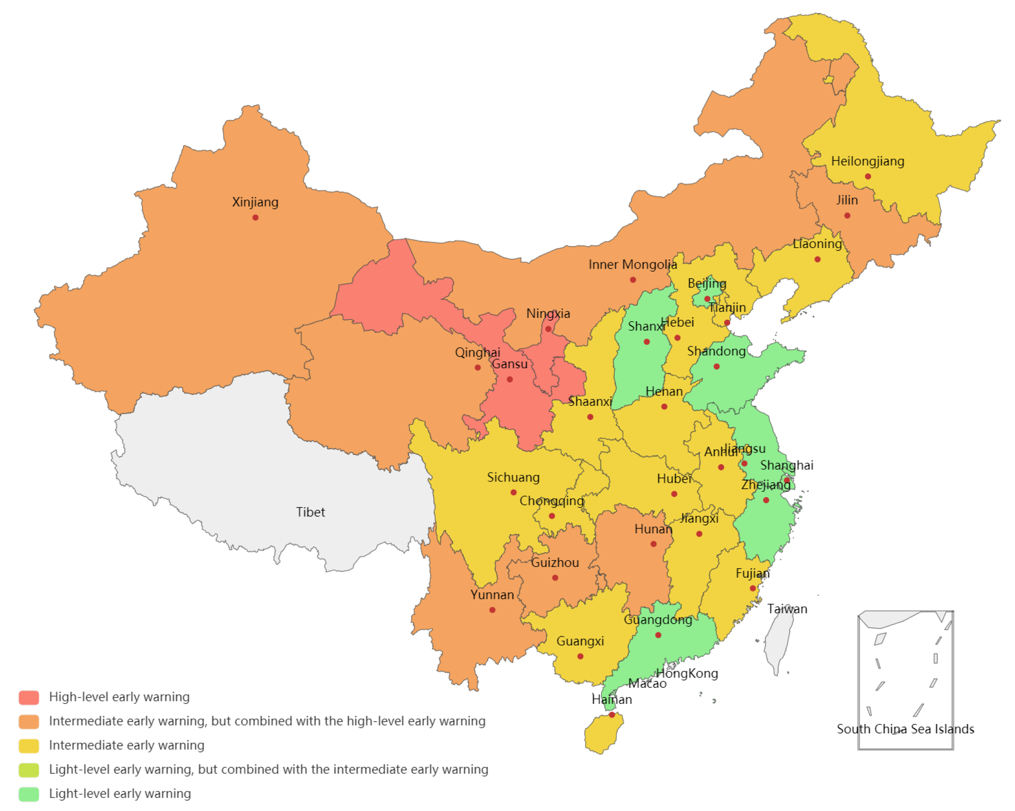
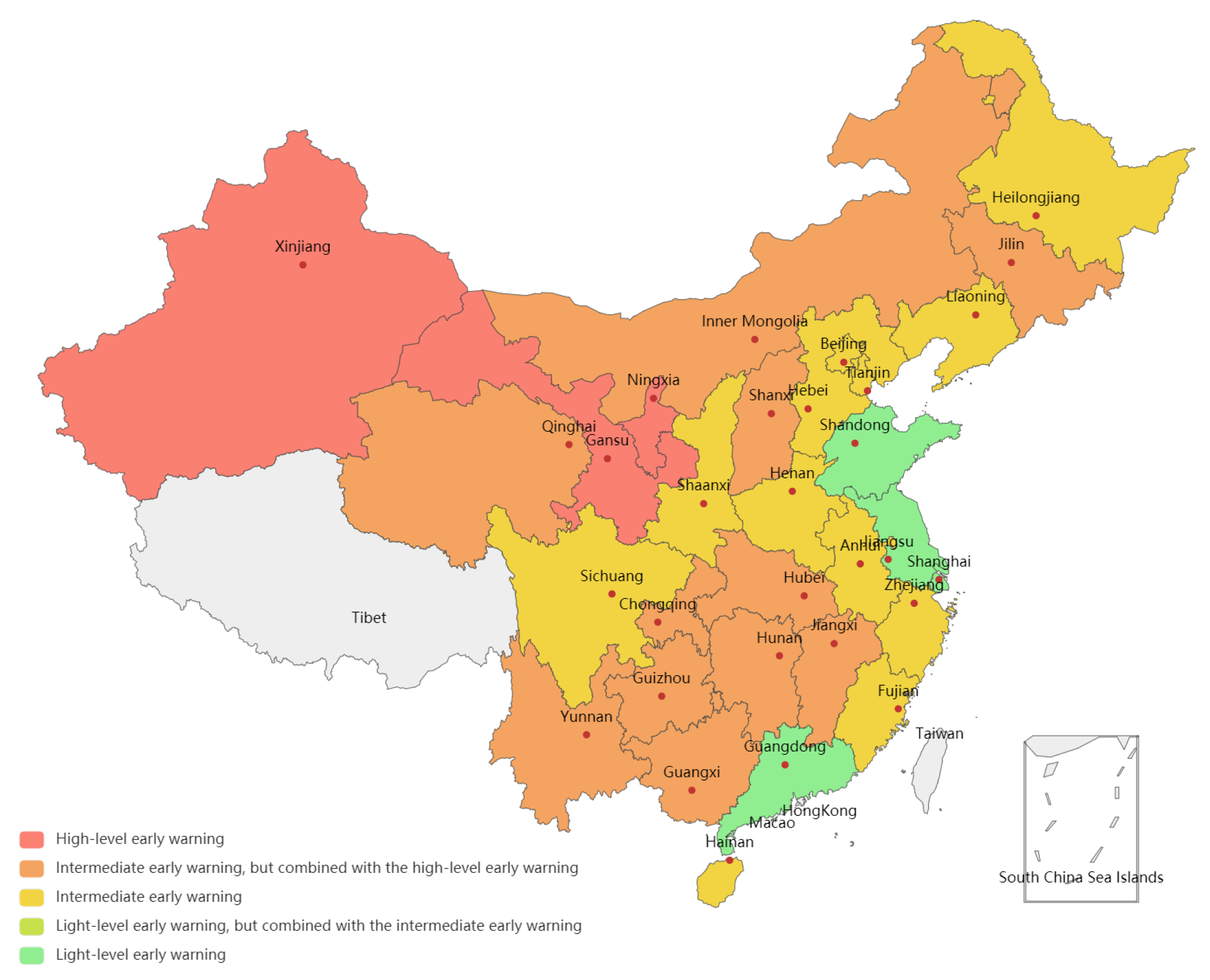
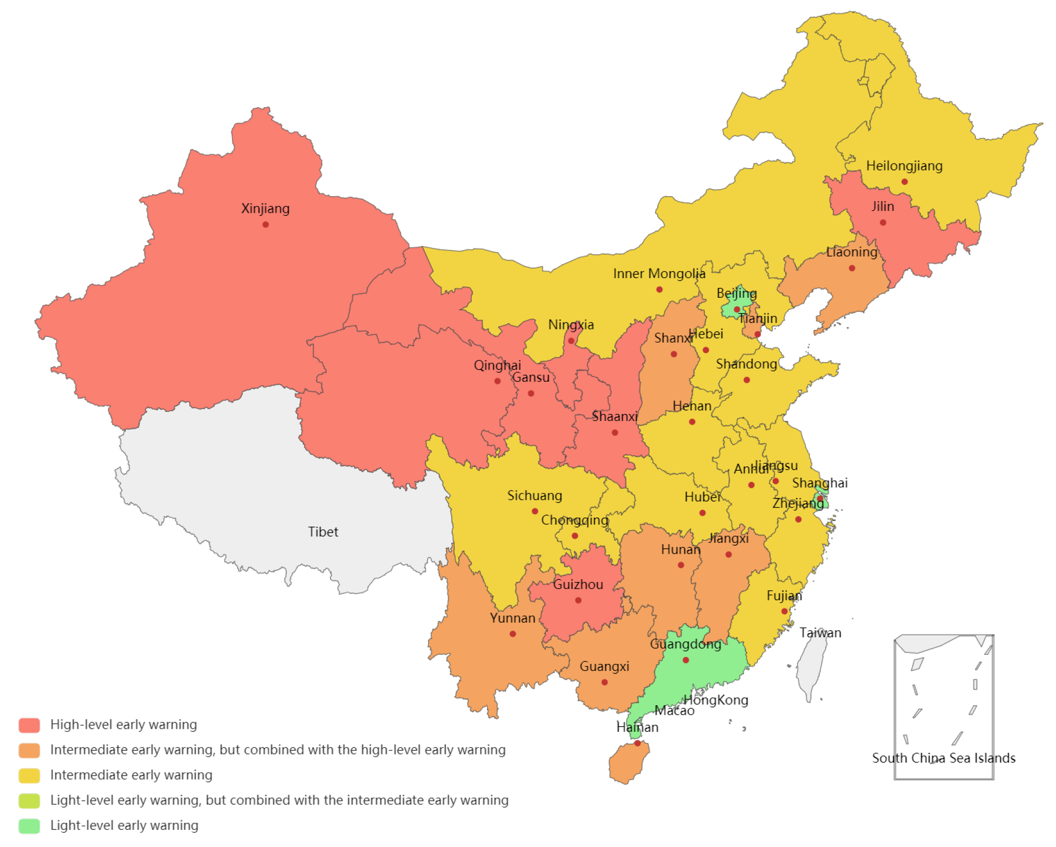
According to the statistical results, from 2017 to 2019, there still existed large financial risks in all provinces and cities in China and, with the passage of time, the number of low-risk areas decreased and the number of high-risk areas increased (see Figure 2, Figure 3 and Figure 4). There were seven provinces or cities whose local finance was within the low-risk zone in 2017, including Shanghai, Guangdong, Beijing, Shanxi, Jiangsu, Zhejiang and Shandong. In 2018, the number of such provinces or cities was reduced by three, with Shanghai, Guangdong, Jiangsu and Zhejiang still existing. In 2019, only three major provinces or city of Shanghai, Beijing and Guangdong stayed on the list. According to the quartile analysis method, only Gansu and Ningxia were within the high-risk zone in terms of local finance in 2017; however, further analysis shows that the number of provinces and cities within the high-risk zone increased to nine: Gansu, Ningxia, Guizhou, Inner Mongolia, Qinghai, Jilin, Xinjiang, Yunnan and Hunan according to the risk prudence principle method. In 2018, Qinghai, Ningxia, Gansu and Xinjiang were classified as the high-risk areas in terms of local finance using the general statistical method, but 10 provinces were added according to the risk prudence principle method, including Yunnan, Shanxi, Hubei, Chongqing, Jiangxi, Jilin, Hunan, Guizhou, Inner Mongolia and Guangxi. In 2019, seven provinces or autonomous regions of Shaanxi, Xinjiang, Jilin, Qinghai, Guizhou, Ningxia and Gansu were classified as the high-risk areas in terms of local finance according to the general statistical method; however, according to the principle of risk prudence, another eight provinces were added, including Shanxi, Hainan, Guangxi, Tianjin, Liaoning, Jiangxi, Hunan and Yunnan; namely, nearly half of the provinces and cities in China were at high risk in terms of local finance.

Based on the summary of the high-risk indicators of high-risk regions in 2019 (

Table 5. Summary of high-risk indicators of the provinces and cities in the high-risk zone in 2019.

Province or City	High-Risk Indicators
Shanxi	Debt expenditure ratio X${}_2$, the elasticity of fiscal expenditure to fiscal revenue X${}_9$, fiscal deficit ratio X${}_{10}$, PPP investment scale X${}_{12}$, fiscal concentration X${}_{14}$, the proportion of tax revenue in fiscal revenue X${}_{15}$, local and national fiscal revenue and expenditure coefficient X${}_{16}$
Tianjin *	Debt burden ratio X${}_1$, debt expenditure ratio X${}_2$, debt-service coverage ratio X${}_3$, financial balance risk coefficient X${}_8$, fiscal deficit ratio X${}_{10}$, PPP investment scale X${}_{12}$, and the proportion of tax revenuein fiscal revenue X${}_{15}$
Liaoning *	Debt burden ratio X${}_1$, debt expenditure ratio X${}_2$, the elasticity of fiscal expenditure to fiscal revenue X${}_9$, fiscal deficit ratio X${}_{10}$, fixed asset investment speed X${}_{11}$, fiscal concentration X${}_{14}$, and the proportion of tax revenue in fiscal revenue X${}_{15}$
Guangxi	Debt burden ratio X${}_1$, debt expenditure ratio X${}_2$, debt-service coverage ratio X${}_3$, financial balance risk coefficient X${}_8$, fiscal deficit ratio X${}_{10}$, fiscal concentration X${}_{14}$, and the proportion of tax revenue in fiscal revenue X${}_{15}$
Hainan *	Debt burden ratio X${}_1$, debt expenditure ratio X${}_2$, financial balance risk coefficient X${}_8$, fiscal deficit ratio X${}_{10}$, fixed asset investment speed X${}_{11}$, PPP investment scale X${}_{12}$, and local and national fiscal revenue and expenditure coefficient X${}_{16}$
Jiangxi	Debt expenditure ratio X${}_2$, financial balance risk coefficient X${}_8$, the elasticity of fiscal expenditure to fiscal revenue X${}_9$, fiscal deficit ratio X${}_{10}$, fiscal concentration X${}_{14}$, the proportion of tax revenue in fiscal revenue X${}_{15}$, and local and national fiscal revenue and expenditure coefficient X${}_{16}$
Hunan	Debt burden ratio X${}_1$, debt expenditure ratio X${}_2$, debt-service coverage ratio X${}_3$, fiscal deficit ratio X${}_{10}$, fiscal concentration ratio X${}_{14}$, proportion of tax revenue in fiscal revenue X${}_{15}$, and local and national fiscal revenue and expenditure coefficient X${}_{16}$
Yunnan	Debt burden ratio X${}_1$, debt expenditure ratio X${}_2$, financial balance risk coefficient X${}_8$, the elasticity of fiscal expenditure to fiscal revenue X${}_9$, fiscal deficit ratio X${}_{10}$, PPP investment scale X${}_{12}$, fiscal concentration X${}_{14}$, and the proportion of tax revenue in fiscal revenue X${}_{15}$
Qinghai	Debt expenditure ratio X${}_2$, financial difficulty coefficient X${}_4$, financial balance risk coefficient X${}_8$, the elasticity of fiscal expenditure to fiscal revenue X${}_9$, fiscal deficit ratio X${}_{10}$, PPP investment scale X${}_{12}$, fiscal concentration X${}_{14}$, the proportion of tax revenue in fiscal revenue X${}_{15}$, and local and national fiscal revenue and expenditure coefficient X${}_{16}$
Jilin	Debt burden ratio X${}_1$, debt expenditure ratio X${}_2$, economic growth rate X${}_5$, fiscal deficit ratio X${}_{10}$, fixed asset investment speed X${}_{11}$, PPP investment scale X${}_{12}$, fiscal concentration X${}_{14}$, the proportion of tax revenue in fiscal revenue X${}_{15}$, and local and national fiscal revenue and expenditure coefficient X${}_{16}$
Guizhou	Debt burden ratio X${}_1$, debt expenditure ratio X${}_2$, financial balance risk coefficient X${}_8$, the elasticity of fiscal expenditure to fiscal revenue X${}_9$, fiscal deficit ratio X${}_{10}$, PPP investment scale X${}_{12}$, fiscal concentration X${}_{14}$, the proportion of tax revenue in fiscal revenue X${}_{15}$, and local and national fiscal revenue and expenditure coefficient X${}_{16}$
Ningxia	Debt expenditure ratio X${}_2$, financial difficulty coefficient X${}_4$, financial balance risk coefficient X${}_8$, fiscal deficit ratio X${}_{10}$, fixed asset investment speed X${}_{11}$, PPP investment scale X${}_{12}$, financial concentration X${}_{14}$, the proportion of tax revenue in fiscal revenue X${}_{15}$, and local and national fiscal revenue and expenditure coefficient X${}_{16}$
Xinjiang	Debt burden ratio X${}_1$, debt expenditure ratio X${}_2$, the elasticity of fiscal expenditure to fiscal revenue X${}_9$, fiscal deficit ratio X${}_{10}$, fixed asset investment speed X${}_{11}$, PPP investment scale X${}_{12}$, fiscal concentration X${}_{14}$, the proportion of tax revenue in fiscal revenue X${}_{15}$, and local and national fiscal revenue and expenditure coefficient X${}_{16}$
Shaanxi *	Debt burden ratio X${}_1$, debt expenditure ratio X${}_2$, debt-service coverage ratio X${}_3$, the elasticity of fiscal expenditure to fiscal revenue X${}_9$, fiscal deficit ratio X${}_{10}$, fixed asset investment speed X${}_{11}$, PPP investment scale X${}_{12}$, fiscal concentration X${}_{14}$, and local and national fiscal revenue and expenditure coefficient X${}_{16}$
Gansu	Debt expenditure ratio X${}_2$, debt-service coverage ratio X${}_3$, financial difficulty coefficient X${}_4$, financial balance risk coefficient X${}_8$, fiscal deficit ratio X${}_{10}$, fixed asset investment speed X${}_{11}$, PPP investment scale X${}_{12}$, financial concentration X${}_{14}$, the proportion of tax revenue in fiscal revenue X${}_{15}$, and local and national fiscal revenue and expenditure coefficient X${}_{16}$

(Note: The provinces and cities marked with “*” are newly added high-risk provinces and cities under the Risk Prudence Principle Method.).

), it can be seen that the debt burden ratio (X${}_1$), debt expenditure ratio (X${}_2$), fiscal deficit ratio (X${}_{10}$), PPP investment scale (X${}_{12}$), fiscal concentration (X${}_{14}$), the proportion of tax revenue in fiscal revenue (X${}_{15}$), and local and national fiscal revenue and expenditure coefficient (X${}_{16}$), were included in the risk factors of a total of ten or more than ten provinces and cities. This shows that there commonly existed risks in the above indicators in the provinces and cities which were within the high-risk zone in terms of financial risks. Among them, the debt expenditure ratio X${}_2$ was even a high-risk factor shared by all high-risk provinces; and the fiscal concentration (X${}_{14}$) and the proportion of tax revenue in fiscal revenue (X${}_{15}$) also occurred in 13 provinces and cities. Based on the above conditions, it can be seen that the main problems in the high-risk regions were concentrated in the following aspects:

First, the heavy debt burden and the high proportion of debt expenditure, which are mainly reflected in two indicators of debt burden ratio (X${}_1$) and debt expenditure ratio (X${}_2$). Among them, all provinces and cities with high-risk local finance have shown that the debt expenditure ratio (X${}_2$) was too high. On the one hand, these regions had already shown a relatively heavy debt burden and the debt pressure there was relatively heavy; on the other hand, the debt expenditure ratio of the above-mentioned regions during the research period was also relatively high, that is, the ratio of new debts of local governments to the local public finance expenditure in the current year was also high; hence, debts were crucial to the local government expenditure. In addition, the fiscal deficit ratio (X${}_{10}$) occurred in the above 15 provinces and cities with high-risk local finance, and all the provinces and cities with the high-risk local finance had an excessively high fiscal deficit ratio at the same time. In the period when China’s economy turned to a high-quality development mode and the period of industrial transformation and upgrade, its economic growth rate began to slow down, resulting in a continuous decrease in the growth rate of local fiscal revenue. At the same time, local governments continued cutting taxes and administrative fees in 2019, thus increasing the financial pressure to a certain extent. At present, the excessive debt pressure has brought huge risks to the local financial and economic development.

Second, hidden debt risks increased. The PPP investment scale (X${}_{12}$) occurred as a high-risk indicator in 11 provinces and cities. PPP projects were an important source of government hidden liabilities, which had accumulated more risks. Some projects lacked long-term consideration and their profit prospects were bleak. Among them, Guizhou, which met the most serious risks, featured the indicator of 71.7%, followed by Yunnan with 48.89%; Xinjiang ranked the third with 43.88%; other provinces scored lower than 40%, and Shanghai the lowest with only 0.06%.

Third, the quality of economic development decreased and the industrial development was unbalanced. Fiscal concentration (X${}_{14}$) and the proportion of tax revenue in fiscal revenue (X${}_{15}$) both appeared 13 times; and these two risk indicators showed up in 12 provinces and cities concurrently. This shows that, in the structure of gross national product, the proportion of local government fiscal revenue was relatively small on the whole, that is, the financial concentration was relatively low, which to a large extent shows that wealth creation value was insufficient. Moreover, the development of the secondary industry and the tertiary industry was not good; in other words, the quality of economic growth was low, with less added value. In the structure of the total fiscal revenue, the proportion of local tax revenue continued decreasing, indicating that the development of the industrial structure guided by the governments was unbalanced. Among them, Hubei Province had the lowest financial concentration, with only 5.52%, and the corresponding dependence on land finance in Hubei Province reached 128.91%. This reflects the characteristics of weak tax collection and high dependence on land finance in Hubei Province. Beijing, Tianjin and Shanghai, three municipalities directly under the administration of the Central Government, showed the best performance in the realization of this indicator, reaching 16.45%, 17.09% and 18.87%, respectively. It completely aligned with the current economic development level. In addition, these two indicators also reflect that local governments had too few sources of fiscal revenue, so it is very necessary for them to expand tax base and enhance taxation ability.

Fourth, the matching degree of local fiscal revenue and expenditure was poor, mainly reflected in the local and national fiscal revenue and expenditure coefficient (X${}_{16}$). The ratio of the two was too large, reflecting the poor matching between local fiscal revenue and expenditure, and the expenditure index was far higher than the income index. At present, most provinces and cities show that their income and expenditure do not match with each other, and the expenditure pressure is too heavy. Among them, Qinghai, Heilongjiang and Hainan are the highest in the ratio, reaching 5.32, 5.22 and 4.80, respectively. In the provinces which featured the lowest ratio, such as Jiangsu, Zhejiang and Guangdong, the ratios were only 0.92, 0.85 and 0.37, respectively. The results show that there is a great imbalance among these regions. Therefore, the Central Government needs to increase the redistribution of transfer payment and strengthen its support for the regions with the higher coefficient values.

Fifth, the hidden dangers of local financial risks were increasing, mainly reflected in the financial balance risk coefficient (X${}_8$). Among them, Qinghai, Ningxia and Tianjin had the highest risk coefficient, while Hebei, Shanghai and Beijing the lowest. The high-risk regions not only rendered heavy debt pressure on local governments, but increased the ratio of household leverage. On the whole, the above regions were faced with greater systemic financial risks, showing that the non-performing loans continued accumulating pressure on the balance sheet and disrupted the normal order of the financial system.

For low-risk regions, there were only three cities of Beijing, Shanghai and Guangzhou which were regarded as low-risk regions in 2019. From 2017 to 2019, both Shanghai and Guangzhou were regarded as a low-risk area, while Beijing became a medium-risk region in 2018 due to the rise of its fiscal deficit ratio. Generally speaking, these three places had performed well in controlling financial risks, and they could still control the level of financial risks well even though the financial risks of most other provinces increased in 2019. By summarizing the non-high risk indicators in 2019 (

Table 6. Summary of non-high risk indicators of the provinces and cities with low risks in 2019.

Province or City	Summary of Non-High Risk Indicators
Shanghai	12 indicators (debt burden ratio X${}_1$, debt-service coverage ratio X${}_3$, financial difficulty coefficient X${}_4$, per capita disposable income of urban and rural residents X${}_6$, unemployment rate X${}_7$, financial balance risk coefficient X${}_8$, the elasticity of fiscal expenditure to fiscal revenue X${}_9$, fiscal deficit ratio X${}_{10}$, fixed asset investment speed X${}_{11}$, PPP investment scale X${}_{12}$, land financial dependence X${}_{13}$, and the proportion of tax revenue in fiscal revenue X${}_{15}$)
Guangdong	10 indicators (debt burden ratio X${}_1$, debt-service coverage ratio X${}_3$, financial difficulty coefficient X${}_4$, economic growth rate X${}_5$, per capita disposable income X${}_6$, unemployment rate X${}_7$, fixed asset investment speed X${}_{11}$, PPP investment scale X${}_{12}$, land financial dependence X${}_{13}$, and the proportion of local fiscal revenue in national fiscal revenue X${}_{16}$)
Beijing	10 indicators (debt burden ratio X${}_1$, financial difficulty coefficient X${}_4$, economic growth rate X${}_5$, per capita disposable income X${}_6$, unemployment rate X${}_7$, financial balance risk coefficient X${}_8$, the elasticity of fiscal expenditure to fiscal revenue X${}_9$, PPP investment scale X${}_{12}$, land financial dependence X${}_{13}$, and the proportion of local fiscal revenue in national fiscal revenue X${}_{16}$)

) and the analysis thereof, we can draw conclusions as follows:

First, compared with medium-risk regions such as Jiangsu and Zhejiang, the low-risk regions had a lower direct explicit financial risk, which was reflected in the debt burden ratio X1 and debt-service coverage ratio X${}_3$. The rapid economic growth and optimized industrial structure had guaranteed the debt repayment in Beijing, Shanghai and Guangzhou. Although Beijing, Shanghai and Guangdong had relatively large debts, they were among the top regions in China in economic performance due to their large economic aggregates. The secondary and tertiary industries there were developed and the per capita disposable income was relatively high. For these regions, the huge economic aggregates and good industrial structure had enabled them to be able to pay for higher debts and resolve debt risks.

Second, compared with the regions with high financial risks, the regions with low financial risks had a lower direct hidden financial risk. This is because Beijing, Shanghai and Guangdong could better manage their fiscal revenue. The investment there was reasonable and the government expenditure structure was relatively optimized. The annual fiscal expenditure and revenue could be arranged more reasonably, and a large enough aggregate could enable these governments to sustain more debts and carry out more PPP projects. Therefore they could determine the scale of debts more reasonably, without using PPP to increase hidden debts, thus reducing the risk of direct hidden debts.

From the local financial risk matrixes in this paper, we can reach the conclusion and predict the trend, which can be basically aligned with the research conclusions by other scholars. According to the survey report released by the Chinese Academy of Fiscal Sciences [14], there were significant regional differences in the domestic local financial capacity: the financial capacity in the eastern region was much higher than that in the western region; moreover, due to the unstable quality of fiscal revenue, the rigid expansion of fiscal revenue and expenditure and the rising financial risks, the local financial risks were on the rise. These two trends can also be seen from the results of the risk matrixes from 2017 to 2019 in this article, which continued spreading, indicating that local financial risks were increasing and could not be ignored. From the results of some provinces, this paper concludes that local financial risks in Guizhou province had developed from the medium-risk level to the high-risk level. This is consistent with the opinions of Yang (2020), that the overall fiscal expenditure in Guizhou Province was faced with greater rigid growth pressure in 2019.

While analyzing the reasons, strategies and future trends of local financial risks, the factors of land finance are the research focus of many scholars. In 2005, the Land Research Group of the Development Research Center of the State Council pointed out that land finance posed great hidden dangers in local finance and urbanization [16]. Land finance affects the change of financial system and the adjustment of industrial structure [17]. Macroeconomic stability and the security of the financial system will be affected by land finance [18]. Land finance and local debts are endogenous in the process of economic growth, which will lead to financial risks and fiscal risks [19]. Therefore, this paper will further study whether land finance has an impact on local financial risks.

3. The Empirical Analysis of the Impact of Land Finance on Local Financial Risks

In this section, we try to empirically investigate the causal effect of land finance on local financial risks. In the process of land transfers, municipal governments serve as a core authority, and the dependences on land finance of different governments vary a lot due to the different development levels and land transfer policies. Thus, it will easily discern the impacts of land finance on local financial risks if the analysis is conducted at prefecture level. Considering the continuity and availability of the data, this paper finally includes a panel data of 178 prefecture-level cities from 2009 to 2017 to make empirical analysis.

3.1. Model Setting and Variable Description

In the empirical measurement of the impact of land finance on local financial risks, we established a basic analysis model and included land finance as the independent variable and local financial risks as the dependent variable to make analysis.

$$\begin{array}{cc}\hfill & {\mathrm{deficit}}_{it}={\alpha }_0+{\alpha }_1\ast {\mathrm{LandDep}}_{it}+{\alpha }_2\ast x_{it}+d_i+d_t+{\epsilon }_{it}\hfill \\ \hfill & i=1,2,3,\dots ,n;t=1,2,3,\dots ,t\hfill \end{array}$$

(1)

Among them, i and t, respectively, represent the region and the year; ${\mathrm{deficit}}_{it}$ is the dependent variable, representing the local financial risk index; ${\mathrm{LandDep}}_{it}$ is a variable reflecting the land financial level of each region, $x_{it}$ represents the other control variables, $d_i$ is a city fixed effect, $d_t$ is a year fixed effect, ${\epsilon }_{it}$ represents an independent and identically distributed random error term, the variance is one, and the mean value is zero.

The financial risk index (${\mathrm{deficit}}_{it}$) of the local government in the model uses the financial deficit ratio as the proxy variable; for local governments’ dependence on land finance, land finance level is chosen as the evaluation index; for the speed of local economic development, the speed of GDP growth is adopted; the level of local economic development is expressed by the GDP per capita; for the local industrial structure, the ratio of the secondary industry to the tertiary industry is used, and the calculation methods for each variable in the model are shown in

Table 7. Variable description and calculation method.

Category	Variables	Explanation	Calculation
Dependent variable	$Deficit$	Financial deficit ratio	(Expenditure–revenue from general budget of local finance)/GDP
Independent variable	$LandDep$	Land financial dependence	Income from land transfers/general budget revenue of local finance
Control variable	$Rsi\_ti$	Ratio of the secondary industry to the tertiary industry	Total output value of the secondary industry/Total output value of the tertiary industry
	$lnpgdp$	Per-capita GDP	Regional GDP per capita
	$ggdp$	GDP growth rate	Regional GDP growth rate
	$lnhp$	Average price of commodity houses	Sales of commodity houses/sold area of commodity houses

:

Data sources of this paper: the total output value of the secondary and tertiary industries, the sold area and sales volume of commodity houses are obtained through the Wind Database, while such data as fiscal budget, fiscal revenue and fiscal expenditure are obtained from the China City Statistical Yearbook (2009–2017). To ensure the accuracy of the calculation results and eliminate the influence due to abnormal values, we winsorize the continuous variables at the 1st and 99th percentiles, with its descriptive statistics shown in

Table 8. Descriptive statistics for variables.

Variables	Observations	Mean	Standard Deviation	Minimum	Maximum
Deficit	1638	0.079	0.059	−0.004	0.284
LandDep	1638	0.449	0.328	0.02	1.571
Rsi_ti	1638	1.33	0.527	0.311	3.38
lnpgdp	1638	10.667	0.559	9.363	11.887
ggdp	1638	10.552	3.581	−2.3	19.4
lnhp	1638	8.496	0.466	7.572	9.969

:

3.2. Empirical Analysis

Based on Formula (1), this paper uses the ordinary least squares (OLS) method for basic regression, and

Table 9. Results of basic regression.

Variables	Deficit	Deficit	Deficit	Deficit	Deficit	Deficit
	(1)	(2)	(3)	(4)	(5)	(6)
LandDep	−0.030 ***	−0.004	0.008 ***	0.008 ***	0.010 ***	0.010 ***
	(−6.34)	(−1.14)	(3.08)	(2.92)	(4.43)	(4.26)
Rsi_ti		−0.012 ***			−0.017 ***	0.007 **
		(−5.51)			(−5.21)	(2.07)
lnpgdp		−0.078 ***			−0.008	−0.071 ***
		(−24.84)			(−1.35)	(−6.36)
ggdp		−0.004 ***			−0.001 ***	−0.001 **
		(−9.35)			(−4.92)	(−2.38)
lnhp		0.001			0.014 ***	0.009 *
		(0.19)			(2.69)	(1.75)
City fixed	No	No	Yes	Yes	Yes	Yes
Year fixed	No	No	No	Yes	No	Yes
Constant	0.092 ***	0.957 ***	0.075 ***	0.068 ***	0.073	0.723 ***
	(36.28)	(32.54)	(66.14)	(36.98)	(1.65)	(6.92)
R${}^2$	0.028	0.491	0.622	0.210	0.198	0.313
F value	40.236	261.734	70.07	25.963	20.106	19.550
Observations	1638	1638	1638	1638	1638	1638

Note: t value is in parentheses, *, ** and *** refer to significance at levels of 10%, 5% and 1%, respectively, and the result indicators in the following tables represent the same.

shows the specific regression results. First of all, without adding any control variables (column 1), the regression results show that the coefficient between land financial dependence and financial risks is significantly negative, which is contrary to our expectation. However, considering that the financial risks of local governments will also be affected by factors such as local economic development level and real estate development, this paper continues to add control variables such as the ratio of the secondary industry to the tertiary industry, the GDP per capita and the average price of commodity houses for further analysis (column 2). The results show that the negative relationship between land financial dependence and government financial deficit ratio is no longer significant.

Secondly, considering that the influence of the land financial dependence at different levels on local financial risks may vary across regions and times, this paper further analyzes the city fixed effect and(or)year fixed effect (column 3–column 6). The results show that the dependence on land finance significantly increases the financial deficit ratio of local governments at the 1% significance level, which indicates to a certain extent that excessive dependence on land finance will increase the financial risk of local governments.

Regarding the influence of other control variables on local financial risks, the results in column 6 show that the ratio of the secondary industry to the tertiary industry significantly increases local financial risks, the level of economic development and economic growth significantly reduces local financial risks, and the level of housing prices significantly pushes up local financial risks. The coefficients of the ratio of the secondary industry to the tertiary industry in column 6 are opposite to those in columns 2 and 5. From the perspective of economic logic and regression results, certain factors that only change over time may have an impact on local fiscal risks but are neglected in column 2 and 5, in which the year are not fixed. Therefore, the results in which year and city are both fixed (column 6) are more convincing.

3.3. Robustness Test

In this paper, the robustness tests are carried out by the following four methods. The regression results from

Table 10. The results from robustness test.

Variables	OLS			IV-2SLS
	lnDeficit	Deficit	lnDeficit	Deficit	lnDeficit	lnDeficit
lnLandDep	0.0152 ***			0.047 ***	0.041 ***	0.041 ***
	(4.120)			(3.55)	(3.50)	(3.49)
L.lnLandDep		0.0132 ***	0.0114 ***
		(2.725)	(2.689)
Contorl variables	Yes	Yes	Yes	Yes	Yes	Yes
City fixed	Yes	Yes	Yes	Yes	Yes	Yes
Year fixed	Yes	Yes	Yes	Yes	Yes	Yes
Constant	0.608 ***	0.679 ***	0.612 ***	0.711 ***	0.639 ***	0.652 ***
	(6.254)	(5.881)	(6.113)	(9.35)	(9.63)	(9.59)
R${}^2$	0.323	0.305	0.317	0.272	0.287	0.286
F	22.92	20.62	22.48	44.09	46.80	45.76
Observations	1638	1456	1456	1456	1456	1424

Note: The dependent variables and the core independent variables are both logarithmized after adding 1 to make the data smoother except in columns 2 and 4. The independent variables in columns 2 and 3 are both lagged by one year. Columns 4–6 are the regression results of IV-2SLS, and column 6 shows the results excluding observations from Beijing, Shanghai, Guangzhou and Shenzhen.

show that the conclusion holds in the robustness tests.

Robustness Test 1: Both the dependent and independent variables are logarithmized to make the data smoother and the results remain robust (column 1).

Robustness Test 2: As the land financial dependence delayed by one period can affect the local government financial risks, but the local debt risk cannot affect the land financial dependence in the previous period, this paper lags both the independent variables and the control variables by one period and adds them to the model, respectively, for recalculation. Although the coefficients in column 2 and 3 are smaller compared to that of column 1, the calculation results prove to be still stable.

Robustness Test 3: The land financial dependence delayed by one period is taken as the instrumental variables of the current land financial dependence, and estimated by the two-stage least square method (2SLS) [20]. The calculation result is still significantly valid and there is no problem of weak instrumental variables (column 4–5). The Cragg–Donald Wald F statistics in columns 4, 5 and 6 are 100.964, 100.964 and 97.853 relatively, indicating there is no reason to doubt the weak instrument variable problem.

Robustness Test 4: Considering that the land policies and borrowing methods of the municipalities directly under the Central Government may be somewhat different from those of other prefecture-level cities, this paper removes the four municipalities directly under the Central Government and carries out the regression again, finding that the calculation results remain stable (column 6).

3.4. Heterogeneity Analysis

The proportions of land finance in local government fiscal revenue vary in the regions with different urbanization rates, which may exert different impacts on their financial risks. To explore the heterogeneity of the impacts of land finance on financial risks for regions with different urbanization rates, we divide the cities to two parts named regions with high urbanization rate versus low urbanization rate using the median urbanization rate of 178 cities in 2013 as the basis of classification. Specifically, the regions whose urbanization rate is greater than the median will be taken as the regions with high urbanization, while the regions whose urbanization rate is lower than the median will be taken as the regions with low urbanization.

The calculation results in

Table 11. Impacts of land financial dependence on local government financial risks in different urbanized regions.

Variables	High Urbanization Rate	Low Urbanization Rate	High Urbanization Rate	Low Urbanization Rate
	OLS	OLS	IV-2SLS	IV-2SLS
L.lnLandDep	0.0091 *	0.0175 ***	0.0254 *	0.0367 **
	(1.827)	(3.131)	(1.752)	(1.968)
Control variables	Yes	Yes	Yes	Yes
City fixed	Yes	Yes	Yes	Yes
Year fixed	Yes	Yes	Yes	Yes
Constant	0.424 ***	1.122 ***	0.434 ***	1.015 ***
	(3.138)	(6.942)	(6.05)	(888)
R${}^2$	0.307	0.381	0.284	0.370
F	12.86	13.71	23.04	30.17
Observations	760	696	760	696

Note: The first two columns are the regression results of OLS model. In addition, the last two columns are the regression results of the IV-2SLS model and the Cragg–Donald Wald F statistics in column 3 and 4 are 42.395 and 47.777 relatively, indicating there is no reason to doubt the weak instrument variable problem.

show that in the regions with a low urbanization rate and a high urbanization rate, local government financial deficit ratio along with the increase in land financial dependence, indicates that there is a significant positive correlation between the two indicators. The results from OLS and IV-2SLS both show that, for cities with lower urbanization rate, the land financial dependence will play a more significant positive role in local government financial risks. It is more likely for the low urbanized regions to depend highly on the land finance to develop due to there being more urbanization space for them. In this case, the local financial risks induced from land finance are more significant for cities with lower urbanization rate. The analysis is based on the results from IV-2SLS model considering that the results from IV-2SLS are more robustness after involving an exogenous variable as instrument variable.

Finally, this paper divides the 178 cities into four regions: eastern, central, western and northeastern. The regression results from

Table 12. Impacts of land finance dependence on local government financial risks for different regions.

Regions	Northeastern Region		Western Region		Central Region		Eastern Region
	OLS	IV-2SLS	OLS	IV-2SLS	OLS	IV-2SLS	OLS	IV-2SLS
L.lnLandDep	0.0690 ***	0.255 *	0.00514	−0.00971	0.00616	0.000329	0.0219 ***	0.0591 ***
	(3.230)	(1.870)	(0.602)	(−0.274)	(1.558)	(0.0237)	(5.531)	(3.769)
Control variables	Yes	Yes	Yes	Yes	Yes	Yes	Yes	Yes
City fixed	Yes	Yes	Yes	Yes	Yes	Yes	Yes	Yes
Year fixed	Yes	Yes	Yes	Yes	Yes	Yes	Yes	Yes
Constant	0.366	2.015	0.703 ***	0.712 ***	0.626 ***	0.629 ***	0.0861	0.0905
	(0.818)	(1.452)	(3.425)	(3.418)	(6.836)	(6.827)	(0.964)	(0.946)
R${}^2$	0.584	0.269	0.125	0.109	0.368	0.364	0.372	0.280
Observations	128	128	200	200	416	416	712	712

Note: The northeastern, western, central and eastern regions in this paper include 16, 25, 52 and 89 cities, respectively. The Cragg–Donald Wald F statistics in column 4, column 6 and column 8 are 9.525, 30.213, 46.879 relatively, indicating there is no reason to doubt the weak instrument variable problem except in column 2, whose Cragg–Donald Wald F statistic is 4.001. However, to maintain the consistency of the models, the instrumental variable in column 2 is not replaced.

reveal that in the northeastern and eastern regions, local governments’ dependence on land finance will have a significant positive effect on financial risks by both OLS and IV-2SLS regression models (columns 1, 2, 7, 8). In addition, the coefficients of the northeastern region are larger than those of the eastern region, indicating that the financial risks derived from land finance are more noticeable for northeastern regions. The phenomenon may be explained by the low urbanization rate in northeastern regions. The average urbanization rate in northeastern regions is 49.72% from 2009 to 2017, which is significantly lower than that of eastern regions with 55.57%.

Meanwhile, for central and western regions, the impacts are nonsignificant. This may be due to the large per capita land area, sufficient land supply and low land prices in the central and western regions, and there is less possibility that local government financial risks arise from land finance. While for the eastern and northeastern regions, land resources are relatively tight and land prices are relatively high. So, it is more likely for these governments obtain funds through land transfers. Hence, local governments’ financial risks will naturally increase followed by the increasing possibility of outbreak of financial risks.

4. Conclusions and Recommendations

From the empirical analysis, there were still great risks in the local finance of all provinces and cities in China from 2017 to 2019. Local financial risks showed an increasing trend in the vertical dimension, which was mostly related to the high dependence on land finance. There were significant differences in the financial risks of different local governments at the horizontal level, so attention should be paid to the rising risk level of local governments in certain regions (such as the western region).

High dependence on land finance will significantly increase the financial risks of local governments, especially in the eastern region where land resources are scarce. In general, attention should be paid to the soaring cost of land expropriation and other major risks implied in land finance. Local governments’ “land financing” model is unsustainable [21]. Through analysis and demonstration, this paper puts forward the following policies and suggestions to prevent local financial risks:

• Design and implement local land finance policies based on local conditions. Local governments should have greater allocation rights in the use of land resources, and land should serve as an important means to regulate local economy [22]. Local governments should formulate land policies which meet the reality of local development.
• Distinguish risk categories and improve the early warning mechanism. The impacts of different types of risks on local financial risks are different. Local governments can actively build a better risk early warning system according to different weights developed based on the impact of different risks.
• Prudent budget management should be conducted to prevent local financial risks. Considering the overall economic downturn and tight fiscal revenue, the financial risk level of each region should be evaluated. The medium and long-term land financial policy should be laid out in advance so as to prompt the governments to take a series of measures to compress the risk areas and eliminate risks.
• Full attention should be given to the high-quality allocation of financial funds to assist the high-quality economic development. Faced with the grim situation that the risks at home and abroad have increased significantly, we should strive to boost the high-quality economic development through high-quality allocation of financial funds; namely, strengthen the security of people’s livelihood and support the stable development of the real economy in a more powerful way, so as to solve local financial risks.

References

- Liu, S.; Jiang, S. Land Finance and Financial Risks-A Case Study from a Developed Area in East China. China Land Sci. 2005, 19, 3–9. [Google Scholar]
- Zhao, Y. Land Finance: History, Logic and Selection. Urban Dev. Stud. 2014, 21, 1–13. [Google Scholar]
- Zhu, Q.; Zhang, M. Land Financial Evaluation Based on the Operational Efficiency of China’s Economic System. Econ. Probl. 2020, 42, 10–18. [Google Scholar]
- Li, Y. Risk Analysis and Reform Suggestions of Land Finance. J. Anhui Agric. Sci. 2013, 41, 9089–9090+9097. [Google Scholar]
- Wu, D. Political Economy Analysis of Land Finance-Based on Marx’s Theoretical Perspective of Land Rent National Debts (National Taxes). Econ. Probl. 2010, 32, 9–12. [Google Scholar]
- Li, Y. Local Government Bonds, Land Finance and Systemic Financial Risks. J. Financ. Econ. 2019, 45, 100–113. [Google Scholar]
- Shen, K.; Zhao, Q. Land Function Alienation and Sustainability of China’s Economic Growth. Ecoomist 2019, 31, 94–103. [Google Scholar]
- Polackova, H. Contingent Government Liabilities: A Hidden Risk for Fiscal Stability; World Bank Publications: Washington, DC, USA, 1998. [Google Scholar]
- Wang, M. Counter-cyclical Adjustment Policies of Finance and Their Risks. Zhejiang Acad. J. 1999, 37, 36–41. [Google Scholar]
- Ma, J. Hidden Fiscal Risks in Local China. Aust. J. Public Adm. 2013, 72, 278–292. [Google Scholar]
- Liao, H.; Fan, R. Tax Distribution System and Local Fiscal Deficit-Model Test Based on Panel Data of the East China. Soc. Sci. Res. 2014, 36, 14–20. [Google Scholar]
- Zou, X.; Mo, G.; Liuyang, Q.; Liu, G.; Chen, H. Research on Risk Assessment and Early Warning of Local Government Land Finance. China Land Sci. 2017, 31, 70–79. [Google Scholar]
- Chen, K.; Arye, L.H.; Gu, Q. Fiscal Re-centralization and Behavioral Change of Local Governments-From the Helping Hand to the Grabbing Hand. China Econ. Q. 2002, 2, 111–130. [Google Scholar]
- Liu, S.; Shi, Y.; Wu, J. Failure of the Institutionalist Public Debt Management Model-Reflection on the Perspective of Public Risks. Manag. World 2017, 33, 5–16. [Google Scholar]
- Liu, S.; Bai, J.; Fu, Z.; Cheng, Y.; Li, C.; Liang, J.; Liang, Q. Be Highly Alert to Risk Deformation and Improve the Ability to Control Risk—General Report on theInvestigation of “Local Financial and Economic Operation in 2017”. Public Financ. Res. 2018, 39, 2–13+30. [Google Scholar]
- Li, J.; Jiang, S.; Han, J.; Liu, S. Land System, Urbanization and Financial Risks-A Case Study from a Developed Area in East China. Reform 2005, 18, 12–17. [Google Scholar]
- Chen, Z.; Chen, L. Changes of Fiscal and Taxation System, “Land Finance” and Economic Growth. Public Financ. Res. 2011, 32, 24–29+134. [Google Scholar]
- Zhang, P. An Empirical Study on the Financial Sustainability of Local Governments in China in the Post Land Finance Era. Reform Econ. Syst. 2013, 31, 131–134. [Google Scholar]
- Liu, N.; Hou, C.; Zhong, Q. Risk Judgment and Response of Local Finance in China. Chin. Public Adm. 2017, 33, 25–29. [Google Scholar]
- Xiang, H.; Wu, J.; Xie, J. Does Local Debts Affect Economic Fluctuation? Chin. Ind. Econ. 2017, 35, 43–61. [Google Scholar]
- Liu, Y.; Chen, J. Land System, Financing Model and Industrialization with Chinese Characteristics. China Ind. Econ. 2020, 38, 5–23. [Google Scholar]
- Xie, Z. Tax Distribution Affects Local Governments’ Land Finance Behaviors. Chin. Chin. Soc. Sci. Today 2020. [Google Scholar] [CrossRef]
Figure 1.
Fiscal revenue and expenditure of both the central and local governments in China from 1995 to 2019.
Figure 2.
Financial risk evaluation results of the provinces and cities in China in 2017.
Figure 3.
Financial risk evaluation results of the provinces and cities in China in 2018.
Figure 4.
Financial risk evaluation results of the provinces and cities in China in 2019.