Energy Crops in Regional Biogas Systems: An Integrative Spatial LCA to Assess the Influence of Crop Mix and Location on Cultivation GHG Emissions


1
Department of Bioenergy, Helmholtz Centre for Environmental Research (UFZ), 04318 Leipzig, Germany
2
Bioenergy Systems Department, Deutsches Biomasseforschungszentrum (DBFZ), 04318 Leipzig, Germany
*
Author to whom correspondence should be addressed.
Sustainability 2020, 12(1), 237; https://doi.org/10.3390/su12010237
Submission received: 22 November 2019
/
Revised: 10 December 2019
/
Accepted: 12 December 2019
/
Published: 27 December 2019
(This article belongs to the Special Issue Life Cycle Management for Sustainable Regional Development)
Abstract
:Anaerobic digestion producing biogas is an important decentralized renewable energy technology used to mitigate climate change. It is dependent on local and regional feedstocks, which determine its sustainability. This has led to discussions on how to alter feedstock for biogas plants without compromising their GHG (Greenhouse gas) saving, one particular issue being the use of Maize silage (MS) as the dominant feedstock. To support this discussion, this paper presents an integrated life cycle assessment of energy crop cultivation for 425 biogas catchments in the region of Central Germany (CG). The simulations for the CG region showed that MS as an effective crop to mitigate GHG emissions per kilowatt hour (GHGculti) was context dependent. In some cases, GHGculti reductions were supported due to higher yields, and in other cases, this led to increased GHGculti. We show that the often-proposed strategy of substituting one crop for another needs to be adapted for strategies which take into account the crop mixtures fed into biogas plants and how they perform altogether, under the specific regional and locational conditions. Only in this way can the trade-offs for lower GHGculti be identified and managed.
1. Introduction
Anaerobic digestion producing biogas is one of the most important decentralized renewable energy technologies, which is heavily dependent on local and regional feedstocks. It is undergoing rapid expansion globally in order to combat climate change and to ensure a secure energy supply [1]. There are a variety of ways in which biogas can be produced, and this varies extensively between countries and even within countries. In Germany, for example, distinct regional differences can be observed for biogas production [2]. While financial incentives under the German Renewable Energy Sources Act have had a strong role in determining what feedstock or combinations of feedstocks are potentially used, German biogas plants are generally planned and built according to available feedstocks [3]. Approximately 92% of substrates used in biogas plants originate from agricultural sources [2], such as livestock manures (solid and liquid) and energy crops, which have a higher energy content [4,5,6].
The most prominent energy crop used is maize silage, contributing approx. 70% to the total mass of energy crops used in biogas plants in Germany. The next prevalent energy crops are grass and cereal (whole crop) silage [2]. Maize silage is the preferred crop due to its technological suitability. Additionally, its high dry matter and energy yields [6] promote it as the most effective crop to mitigate greenhouse gas (GHG) emissions [7,8]. However, the GHG emissions for cultivating energy crops can contribute between 50–70% of the total GHG emissions associated with biogas production [9,10]. This among other reasons has led to the cultivation of energy crops for biogas to undergo review in Germany [11]. Indeed, discussions on how to alter the feedstock mix being supplied to biogas plants, as well as how to reduce the dependency on maize silage in the feedstock mix, without compromising the GHG saving potential, are gaining momentum [4,5,8,12].
The method employed for estimating such GHG emissions is usually life cycle assessment [13,14,15]. There have been several life cycle assessments to date of biogas systems focusing on various aspects such as: Technical efficiency, system boundaries, and credits [16,17,18,19,20,21,22]. However, few have investigated biogas production within a region, and those that did have done so with limited inclusion of regional variability and the effects of feedstock mixtures (i.e., combinations of energy crops) on the associated cultivation emissions [18,21,23]. Only one study was found to assess regional biogas production as a function of feedstock per hectare land used (kgCO2eq/ha) and as a function of the energy generated (kgCO2eq/kWhel). This is important to point out, as it is debated in the LCA community whether bioenergy assessments should be conducted per hectare input of energy crop or per energy output [13]. The distinction being that, per function of energy crop used provides a better idea of efficient land use options and mitigation strategies for reducing cultivation emissions from energy crops (e.g., yields vs. fertilizer). Whereas, the balances provided per function of energetic output allows comparison with other energy systems.
One potential solution to tackle the limitations of these previous studies has been the development of regionally contextualized life cycle concepts [24] and modelling approaches [25] to assess bioenergy production for an entire region. For such regional modelling, the functional unit is not an issue, as the regional cultivation of energy crops and energy generation are assessed in an integrative manner through the use of bioenergy catchments and spatial indicators. A recent study by O’Keeffe et al. [10] has used the RELCA (a REgional Life Cycle inventory Assessment) approach [25] to model the greenhouse gas mitigation potential of 425 biogas plants and their energy crop catchments operating in the region of Central Germany (CG). With their integrative approach, they identified the need to examine in more detail the effects of feedstock mixtures being used within biogas catchments and the locational factors which influence the cultivation emissions of energy crops and hence the GHG mitigation potential of regional biogas systems.
The aim of this paper, therefore, is to examine in more detail the cultivation phase of the regional biogas life cycle outlined in [10] to: (1) Assess the GHG emission profiles of the major crops used in the CG biogas catchments per hectare of land used (CultiEmis) (kgCO2eq/ha), as well as the regional distribution of CultiEmis associated with the cultivation of biomass for biogas production; (2) to investigate the effect of energy crop mixtures, particularly the share of maize silage, on the cultivation emissions of the regional biogas catchments as a function of energetic output GHGculti (kg CO2eq/kWhel), and (3) to investigate the effects of location (e.g., soil, climate, crop yields) on the cultivation emissions of the regional biogas catchments as a function of energetic output (kg CO2eq/kWhel), to help identify potential options for altering the feedstock mix.
2. Materials and Methods
2.1. Regional Description—Central Germany (CG)
The CG region has mainly a temperate climate, with northern areas having on (50 year) average relatively higher mean annual temperatures (9–10 °C) and lower mean annual rainfall (450–600 mm). The more mountainous regions of the south have lower mean annual temperatures (6–7 °C) and higher mean annual rainfall (600–1000 mm) [26]. In 2010 approx. 500,000 hectares were devoted to cereals (Rye, Barley, and Triticale), with approx. 550,000 hectares under grassland, as well as approx. 200,000 hectares devoted to maize silage, of which approx. 27% was found to be used for biogas production [27,28,29].
During the temporal scope of this study, there was an estimated 570 biogas plants in operation in the CG region. This includes plants using municipal organic wastes (e.g., domestic food waste), industrial wastes (e.g., distillery wastes), and agricultural plants (using energy crops and slurry) [2,30]. The main energy crops (EC) being used by the agricultural plants included; maize silage (MS), grass silage (GS), and small amounts of cereal grains (Cer)—Rye, Barley, and Triticale.
2.2. Overview of Life Cycle Approach—RELCA
The RELCA approach of O’Keeffe et al. [25] was applied (see Supplementary Materials S1.1 for overview of modelling steps). The regional foreground was set to the eastern German region of Central Germany (CG), which consists of three federal states, or “Bundesländer” (Figure 1); Saxony, Saxony-Anhalt, and Thüringen. O’Keeffe et al. [10] have already used RELCA to assess the full regional life cycle for 425 agriculturally based biogas plants operating in CG. However, in this paper we focus only on the cultivation of energy crops being used within regional biogas catchments (no system expansion through credits). The scope for individual biogas catchments (n = 425) is from field-to-field gate. However, the conversion step is indirectly taken into account through the assignment of crop catchment areas to biogas plants (see Section 2.6), as well as the use of the digestate from the associated biogas plants (i.e., part of fertilizing regime).
2.3. Functional Unit Combined with Spatial Indicators
The total GHG emission for cultivation (GHGculti) for each biogas plant is the product of all constituent grid cells within the biogas catchment (Bcat) calculated as kilogram equivalents of CO2 per (net) kilowatt hour electricity produced (kgCO2eq/kWhel) and for the analysis presented here, is the overall functional unit. However, we want to investigate the GHG performance of Bcats based on the shares of energy crops. To do this, we use two key spatial indicators in combination with GHGculti to compare across the Bcats and to help understand important underlying geographical factors.
The first is the emission intensity (EI) of the Bcats (kgCO2eq/ha). It differs from the CultiEmis (kgCO2eq/ha) estimated for the individual energy crops (Section 3.1), in that it is the medianed CultiEmis of the crop mixtures associated with a specific Bcat and is unique to the Bcat. If, for example, a Bcat has a high median EI, this means that based on the location, many of the constituent grid cells of the Bcat were associated with a high CultiEmis.
The second indicator is the size of the biogas catchment area or the land area demand (LADBp) per energetic output of the particular bioenergy plant (ha/MWel). It is a form of direct land use footprint (Equation (1)). This spatial indicator is important, as the total GHGculti for each Bcat is the product of all constituent grid cells within the Bcat, i.e., total catchment area (LUTotBp) calculated as equivalents of CO2 per (net) kilowatt hour electricity (NEBP) produced (kgCO2eq/kWhel). Therefore, the more land area being used (greater number of grid cells) then a greater cumulative sum of emissions is more likely, depending on the location.
Both EI and LAD of a Bcat are related to the yields of the associated catchment energy crops and installed capacity of biogas plant, but not always linearly, due to different locational factors such as climate, soils, and crop combinations (see S1.2 in Supplementary). The combination of these two spatial indicators, which are land and location based, will provide us with a better understanding of the mitigation potential of the biogas systems as a function of energetic output (kgCO2eq/kWhel) because their product also equals the total GHGculti found for a particular biogas catchment (Equation (2)).
2.4. RELCA Step 1: Crop Allocation Modelling (CRAM)
The crop allocation modelling or CRAM approach of Wochele et al. [31] was implemented to determine the potential regional distribution of the different crop types; maize silage (MS), grass silage (GS), and cereal grains (Cer), which were used in regional biogas production for 2010/2011 (for more details, see S1.3 in Supplementary).
2.5. RELCA Step 2: Biogas Conversion Systems
In collaboration with the Deutsches Biomasseforschungszentrum (DBFZ), representative model agricultural biogas plants for the CG region were developed [10]. These model biogas plants were based on two characteristics relevant for the German Renewable Energy Sources Act (EEG): (1) Size classes (i.e., installed capacity kW), and (2) dominant feedstock (Fi), i.e., either animal manures or maize silage. Nine model biogas plants or clusters were identified for the CG region, and these were used to generate the LCIs (life cycle inventories) for 425 agricultural biogas plants (see S1.4 in Supplementary). For ease of discussion, the nine clusters described in O’Keeffe et al. [10] will be aggregated further into two classes, biogas catchments belonging to slurry dominant clusters (SLdom), and energy crop dominant (ECdom) clusters (Table 1). The SLdom clusters used relatively little energy crops (<20% EC of mass input), whereas the ECdom clusters used significantly higher energy crops (>60% EC) (see [10] and S1.4 in Supplementary for more detail).
2.6. RELCA Step 3: Biogas Catchment Modelling
Once the feedstock demand for each biogas plant was estimated, catchments were modelled using MATLAB generated scripts and the approach outlined in O’Keeffe et al. [25]. The demand (Fi,p) for each cultivated feedstock type (i.e., MS, Cer, GS, see S1.4 in Supplementary) was used to generate the catchments, which grew in size until the demands of all feedstock types were satisfied for each of the biogas plants (n = 425) modelled, in one simulation run (Equation (3)). However, if a grid cell from an allocated crop was closer to one biogas plant over another, that grid cell was allocated to the closest biogas plant, in order to avoid catchment area overlap [32]. The associated land area for each feedstock (LAFi) was then summed to calculate the total catchment area for each biogas plant (LUTotBP), see S1.5 in Supplementary for overview of land demand modelled.
2.7. RELCA Step 4: Life Cycle Inventory for Biomass Management
Once the catchments had been delineated (Figure 1), the cultivation management and the associated cultivation emissions were calculated per hectare and per kilowatt electricity produced for each constituent grid cell of a Bcat using MATLAB scripts (see [25]). All flows relating to biomass cultivation were included for one harvest only, until just after harvesting for the biogas plant. The operational year for biogas production was assumed to be from the point of harvest in autumn 2010, through to the autumn 2011, as this was the first-time frame for which the most complete data (land use and biogas technologies) was available.
2.7.1. Nitrogen (N) Management and Spreading of Digestate
The recommended nitrogen application and digestate rates were calculated assuming best farming practices and were based on yields and different geographical considerations (e.g., climate, soils, and agricultural suitable index assigned to a grid cell) for energy crops and grasslands (see S1.6 in Supplementary for details).
2.7.2. Other Farm Management—Auxiliary Inputs
The fertilizer application rates for phosphors (P) and potassium (K) were determined based on yields and off take. The inventory data for crop protection products and recommended dosages were also determined for the region (see S1.6 in Supplementary for details).
2.7.3. Field Machinery Operations
2.8. Cultivation Emissions
2.8.1. Soil Emissions (Direct)—Soil N2O
Nitrous oxide emissions (N2O-direct and indirect) from the cultivation of each energy crop was calculated for each constituent grid cell of the Bcats using a Tier 2 approach according to the German national guidelines [34] and using the emission factors (EF) derived by Brocks, et al. [35] (see S1.7 in Supplementary for details).
2.8.2. MachineOpsEmis (Direct and Indirect)
Emissions associated with field machinery operations (MachineOpsEmis) are outlined in [10].
2.8.3. Non-Regional—Indirect Cultivation Emissions (AuxillaryEmis)
All non-regional, upstream emissions were attributed to each constituent grid cell of a Bcat and are outlined in [10].
2.9. Statistical and Spatial Analysis
Emission profiles were generated for each crop (MS, Cer, GS) and for each biogas cluster (see S1.4 in Supplementary for explanation of clusters) using MATLAB 2017b Statistics and Machine Learning Toolbox™ (MATLAB). The emission profiles for the individual energy crops (Figure 2) refers to the distribution of CultiEmis (kgCO2eq/ha) determined for each energy crop grid cell, estimated across all biogas catchments. The emission profiles of Figure 3 and Figure 4 refer to the distribution of emissions determined for each of the Bcats analyzed within a cluster. Significant differences between different regional clusters were tested in R studio [36], using a Kruskal Wallis test (p < 0.05) and the post hoc test, Wilcoxon pairwise comparison, with a Holm correction, as the data was found to be nonparametric.
Using ESRI ArcGIS® [37], a hotspot analysis (Getis Ord Gi) was carried out with a spatially weighted matrix (K nearest neighbor, n = 8), to identify the regional distribution of statistically higher (“hotspot”) or lower (“coldspot”) CultiEmis associated with the regional energy crop cultivation for biogas (kg CO2eq/ha). A further hotspot analysis was done to identify the regional distribution of statistically higher or lower crop yields.
Furthermore, for SLdom and ECdom, those Bcats with the significantly lowest (less than the 10th percentile) and significantly highest GHGculti (kgCO2eq/kWhel) (greater than 90th percentile) were determined. Summary statistics were generated using MATLAB 2017 [38] to profile their underlying geographical parameters. This was done to understand potential locational trade-offs between cultivation emissions, land use, and energy output. All boxplots, bar charts, were produced using MATLAB 2017 [38]. All maps were produced using ESRI ArcGIS® [37].
3. Results
3.1. Energy Crops—CultiEmis
3.1.1. Crop GHG Emission Profiles
The RELCA simulated median CultiEmis for MS was found to be significantly higher (median = 2708 kgCO2eq/ha) than the median CultiEmis found for Cer and GS, of 1662 kgCO2eq/ha and 1573 kg CO2eq/ha, respectively (Figure 2). These results are comparable to the literature, for which higher GHG emissions associated with MS cultivation for biogas has already been shown, in comparison with grass silage [4], sugar beet [8], and cereals [39]. Although the ranges and aspects included in such studies varies widely.
3.1.2. Contribution Analysis
For ease of discussion, we focus on nitrogen related cultivation emissions only, as O’Keeffe et al. [10] found these accounted for 46–59% of the total GHG balance (see S1.8 in Supplementary for additional contribution analysis).
Soil N2O contributes significantly to the GHG balances of different energy crops, and is dependent on the amount of nitrogen fertilizer applied and locational factors such as soil and climate [13,24,40]. For CG, soil N2O contributed between 58–88% of the CultiEmis (kgCO2eq/ha), depending on the crop. For the RELCA simulations, MS had the significantly highest range of soil N2O emissions, from 1.83–8.87 kg N2O_N/ha (median = 3.2 kg N2O_N/ha). Cer had a significantly lower N2O_N emission range, from 0.74–4.65 kg N2O_N ha−1 (median, 1.56 kg N2O_N/ha). GS was found to have the significantly lowest N2O_N emissions, ranging from 0.98–5.27 kg N2O_N/ha, with a median of 1.57 kg N2O_N/ha. The most up to date Tier 2 level approach was used, and these simulated values fall within the ranges found within the literature, and are therefore considered to be plausible (see S1.9 in Supplementary).
In comparison to Soil N2O, (chemical) fertilizer N contributed relatively little to the CultiEmis (4–12%) and was zero for GS and Cer, where the N demand had been met by the digestate applied. For MS, due to its higher N demand, only 26–52% of the N demand could be met with digestate. This meant that MS had the greater chemical N fertilizer demand. Therefore, with both the higher direct N emissions (Soil N2O) and higher indirect emissions (production of chemical N fertiliser) MS was found to have the highest CultiEmis (kgCO2eq/ha).
3.1.3. Spatial Distribution of CultiEmis
In the CG region, there was a tendency for significantly higher CultiEmis in the central and western areas (hotspots) (Figure 3). This is where yields and hence N fertilizer application rates were relatively higher for all crops. In locations to the north, east, and south, a tendency for significantly lower CultiEmis was observed (cold spots). These were areas with significantly lower yields, and thus lower N fertilizer application rates. The spatial trend of high and low CultiEmis corresponded with those found for the N2O emissions (see S1.7 in Supplementary). However, while in the north and in parts of the south had in general significantly lower N2O emissions, pockets of significantly higher N2O emissions were also found (Figure 3). This is due to these areas having the geographical and climate conditions which resulted in higher N2O emission factors (EF) (see S1.7 in Supplementary). The spatial trends for all crops, MS, Cer, and GS had similar trends to that shown in Figure 3.
3.1.4. Hypothesis for GHGculti (kgCO2eq/kWhel) Based on Crops’ CultiEmis (kgCO2eq/ha)
From the contribution and spatial analysis of the different crops’ CultiEmis (kgCO2eq/ha), we would now hypothesize that: (1) Those Bcats with a higher share of MS should have a tendency for higher GHGculti (kgCO2eq/kWhel); and (2) Bcats found in the central west areas of the region should have higher GHGculti (kgCO2eq/kWhel) than those operating in the north, east, and southern parts of the region. We test these two hypotheses in the next sections below.
3.2. Effect of Crop Mixtures on Biogas Catchments GHGculti
In the previous Section, we have investigated the GHG emissions associated with the cultivation of the different energy crops medianed across all Bcats for the CG region. In this Section, we want to investigate the GHG performance of Bcats as a function of net energetic output (i.e., kgCO2eq/kWhel) and how crop shares, particularly MS, within the associated catchments can influence their GHG performance. To do this, we first aggregate the Bcats into Slurry dominant (SLdom) and Energy Crop dominant (ECdom) clusters (see S1.4 in Supplementary for descriptions). We then use the two key spatial indicators, EI (kgCO2eq/ha) and LAD (ha/MWel) to help understand important underlying geographical factors and to compare across the clusters. SLdom clusters had a large share of feedstock contributed from animal manures, whereas, for ECdom clusters a large share came from energy crops (Table 1). Therefore, for the purpose of clear and fair discussion, we will not make direct comparisons between the Bcats associated with ECdom and SLdom clusters.
3.2.1. SLdom Biogas Catchments
For Bcats associated with SLdom clusters, the cultivation of energy crops contributed between 52–56% of the total emissions [10]. The GHGculti ranged from 0.086 to 0.137 kgCO2eq/kWhel. Based on MS shares in the crop mix, we would expect GHGCulti (high to low median) to be as follows: CL8 > CL4 > CL7 > CL2 > CL1. However, we get the following order of: CL4 > CL8 > CL7 > CL1 > CL2, with Bcats associated with CL2 having the significantly lower GHGculti (Figure 4A).
Although the EIs of biogas catchments in CL2 are significantly higher than CL1 (Figure 4C), the effect of significantly lower LADs (Figure 4D) counteracts this, resulting in the overall significantly lower GHGculti for CL2 (Figure 4A). The higher LADs of CL1 relates to the share of Cer in the Bcats feedstock mix. For CL1, Cer contributed approx. 60% of the total land area demand of the Bcats, unlike those of CL2, for which Cer contributed on average only 36%. What this means is that by requiring a greater area to supply the feedstock, the catchments of CL1 had a greater summed volume of GHG emissions per kilowatt hour (Figure 4B), and leading to the increased GHGculti, emissions and it’s poorer than expected performance. For CL4, although with significantly lower EI values, the slightly higher LAD values (not significant) than that of CL8 resulted in the overall median GHGculti of CL4 to be higher (see S1.10 in Supplementary for further discussion).
3.2.2. ECdom Biogas Catchments
For Bcats associated with ECdom clusters, the cultivation of energy crops was found to contribute between 64–67% of the total emissions [10]. Again, based on the share of MS in the feedstock mix of these Bcats, we would expect the GHGculti to rank, from high to low, in the following order: CL6 = CL9 > CL3 > CL5. However, they have the opposite rank of: CL5 > CL3 > CL6 > CL9. Therefore, to pick one clear comparison, why is CL5 performing so poorly and CL9 so well?
The median EI of the Bcats of CL5 (Figure 5C) was the highest (non-significant), but these catchments also had the lowest median LADs (Figure 5D), but were not low enough to counteract the higher EIs (Figure 5C), thus resulting in the poorer than expected performance of CL5. In the case of CL9, the associated biogas catchments had relatively lower EIs (Figure 5C) and although the LADs were slightly higher than for CL5 (Figure 5D), the lower EIs counteracted this and led to the lower GHGculti of CL9 (see S1.10 in Supplementary).
3.2.3. The Effect of Crop Mixtures and the Role of MS on GHGculti Performance
From the analysis of biogas catchments (Bcats) associated with SLdom and ECdom clusters, we see that the overall GHGculti of these Bcats is not entirely dependent on the emission intensity of the dominant energy crop, MS, but is related to the share of the crops in the feedstock mix. This is particularly apparent with the use of crops like cereals, as their relatively low yields result in greater catchment sizes (i.e., bigger LAD values). Additionally, further underlying locational factors play a role in the GHGculti performance, and we analyze this next.
3.3. Location Effects on Biogas Catchments
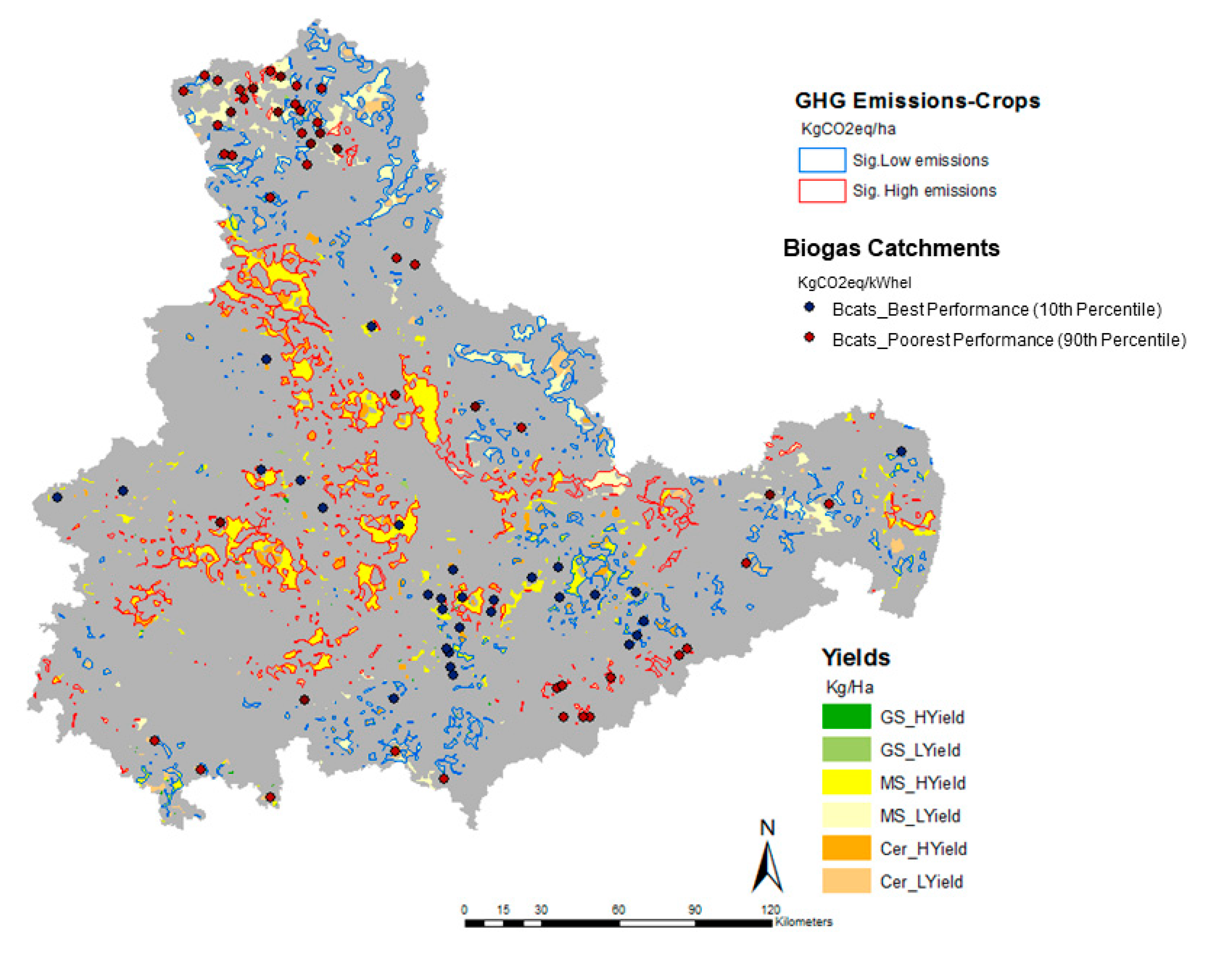
The locational hypothesis based on CultiEmis (kgCO2eq/ha) of crops in Section 3.1.3, is in general the opposite of what we see for GHGculti. From the CultiEmis analysis, we did gain some insights into potential EIs for the regional Bcats, with catchments found in areas denoted blue having low EIs and catchments found in the red areas having higher EIs (Figure 6). However, as seen in Section 3.2, the overall GHGculti of a Bcat not only depends on its EI, but also on the volume of cumulative emissions, i.e., the land areal demand (LAD) of the catchment. Location plays an important role in the balance between these two indicators and hence on the GHGculti.
3.3.1. North, East, and Southern Border Locations (Poorest Performing Bcats)
In the north, east, and southern border locations of the region, RELCA simulations showed Bcats (SLdom and ECdom) to be operating with significantly higher GHGculti (greater than 90th percentile). The Bcats with the significantly highest GHGculti are found in both blue and red demarcated areas with differing locational factors for their significantly higher GHGculti (Figure 6).
All biogas catchments in the blue locations (N, S, E) were found to have overall lower yields (MS 28% lower than the median) (see S1.11 in Supplementary for locational profiles) and lower N fertilizer demand. This combined with lower N2O EFs resulted in Bcats in these locations to have lower EIs (kgCO2eq/ha). However, the lower yields, led to relatively larger LADs (see S1.11 in Supplementary). This resulted in these Bcats to have significantly high GHGCulti, the opposite GHG performance expected when basing it on the feedstock alone, as in Section 3.1.3.
Bcats found in the red locations (north and south) had differing locational factors leading to their significantly higher GHGCulti (Figure 6). In the north (mostly ECdom catchments), the MS yields were found to be lower than the median yields (<17%) and with higher N2O EFs; these Bcats had higher associated EIs. Therefore, the combination of lower yields resulted in larger LAD values (i.e., greater catchment areas, 6% less than the median) and higher EIs, leading to significantly higher GHGculti emissions than the median. Bcats in the southern border locations had the highest N2O EFs, but with relatively low LADs, due to relatively good MS and GS yields (i.e., close to the median). However, for these Bcats, the EIs were so high they could not be buffered by low LADs, and this resulted in the significantly higher GHGculti (see S1.11 in Supplementary).
3.3.2. Central and South-Central Locations (Best Performing Bcats)
RELCA simulations showed Bcats to be operating with significantly lower GHGculti (less than 10th percentile), mostly in the central and south-central areas of the region. The opposite of what was expected. The central area was predominantly demarcated red for higher CultiEmis, the southcentral area identified as blue, significantly lower CultiEmis. For all Bcats with significantly low GHGculti emission, regardless of the location type (i.e., red or blue), they had relatively higher yields for MS and Cer (see S1.11 in Supplementary).
For Bcats in the south-central part of the region (blue), although associated with a relatively higher N fertiliser demand, lower N2O EFsresulted in lower emission intensities (EI) (S1.11 in Supplementary). This, combined with lower LADs, resulted in the most optimum conditions and hence the significantly lower GHGculti (KgCO2eq/kWhel). Bcats in the central areas (red) were found to have much higher yields and hence lower LADs, and could counteract the higher catchment EIs. This resulted in these biogas catchments to have significantly lower GHGculti (see S1.11 in Supplementary).
It must also be noted, that although highly dependent on EC feedstock, ECdom catchments in these central locations had GHGculti emissions similar to some of the worst performing SLdom plants, which had a much lower demand for energy crops. We mention this not to compare between them, but rather to point out the effect location can have on the GHGCulti performance. What this shows, is that from a GHGculti point of view, if the conditions are optimal, a higher volume of energy crops does not necessarily result in an overall higher GHGculti (see S1.11 in Supplementary). However, it must also be noted that a higher volume of energy crops could also result in a higher environmental burden (e.g., reduced soil quality, eutrophication), and this should also be a consideration for examining alternative feedstocks (this analysis is outside the scope of this paper).
4. Discussion
4.1. Location Types and Opportunities for Altering Feedstock Mix in CG
From the spatial analysis of the biogas catchments we identified two extreme location types, as well as locational trade-offs for biogas plants operating within the CG region. These trade-offs are between lowering the land areal demand of a biogas catchment (i.e., lower LAD values due to higher yields) versus lowering its emission intensity (i.e., reducing the nitrogen fertilizer demands, often resulting in lower yields), which all depend on either favorable or unfavorable geographical and climatic conditions (e.g., leading to high or low N2O emissions). Determining location types and their associated trade-offs can help to identify opportunities for altering feedstock mix for biogas production, and thus help to reduce the GHGculti (kgCO2eq/kWhel) for the region. We provide two brief examples of this.
Location type 1—Low EI and high yields: These optimum locations have the best opportunity for diversification of feedstock mix, as these areas are not entirely restricted by balancing the trade-offs of increasing catchment size (i.e., increase in LAD) and the potential for generating higher EIs (e.g., higher nitrogen fertilizer for higher yields). Therefore, crops such as grass silage (GS) with lower yields than MS could be an option for locations like these.
Location type 2—High EI potential and low yields: In areas like these, the mitigation potential of the biogas (field-to-CHP) production can drop by 11–20%, depending on the feedstock mix, e.g., SLdom or ECdom. Bcats associated with ECdom clusters are far more sensitive to these least optimum locations, due their higher dependency on energy crops. Therefore, it could be recommended that for such locations, crops which have a relatively similar or a higher yield than MS (both dry matter and methane), but with a relatively lower N demand should be considered. In this way, aiming to optimize between potentially reducing the EI, while trying to maintain or limit the increase in the LADs of the biogas catchments. The use of cereal grains should be done sparingly in these location types, if used at all, due to the relatively low yields (i.e., increases LAD). Additionally, where possible, another option could be to reduce the dependency on energy crops altogether and substituting instead with locally available residual/by-product feedstocks (e.g., domestic organic waste, molasses).
For the Central German (CG) region simulations, it was identified that the majority of biogas plants and their catchments were found in location types which had, relative for the region, average to high EIs and average to high yields (resulting in a large LAD range). The challenge for altering feedstock mixtures in these areas would be to find the trade-off between lowering the nitrogen fertilizer to reduce the EIs, while not generating too much additional land areal demand (i.e., higher LAD values due to lower yields). In these locations, Maize silage could support a lowering of the GHGculti with its higher yields; however, the dominance of MS would still need to be reduced in catchment locations tending towards higher EIs. The reason being that the high N fertilizer demand of Maize silage could exacerbate the EIs of the biogas catchments so much that the lower LAD value has no effect in reducing the GHGculti. This was observed for some biogas catchments.
For the CG region, several crops have been proposed by the regional agricultural authorities for diversifying and enhancing the feedstock mix of biogas plants and their catchments. These include crops such as whole crop silage (cereal), sugar beet, and sorghum [29,41,42]. These crops were selected in general due their compatibility to the crop rotations of farmers and their comparable methane yields to MS; albeit in some cases it could be between 15%–30% lower than MS [29]. In the case of sugar beet, this was identified as having potentially much higher methane yields and naturally much higher harvest yields (> +20t/ha), and is seen to potentially have a bigger role in the future [11]. However, sugar beet is not without its own agronomic challenges, such as suitability within crop rotations and soil loss [43].
Non-annual crops proposed included grassland and Silphie. The latter could be, once planted, harvested each year for up to 15 years. However, if farmers would dedicate large areas to Silphie, while removing the associated land out of rotation for other cropping products (e.g., livestock systems, market crops), is difficult to answer. With regards to grassland, although the methane yields are slightly lower, in some cases in CG, the yields were comparable to MS, and indeed the emission contributions were 2–3% lower than its energetic contribution. That being said, some studies have suggested that due to the relative higher methane yields and the lower costs of producing MS, GS is not an economically competitive option [4].
However, to test the viability of changing feedstock mixtures being feed into biogas plants would require further, more in-depth investigations (i.e., field studies, more detailed scenario analysis) to determine the feasibility of using these different crops in different proportions within a biogas catchment, while also taking into account the important locational factors which would influence EIs and LADs of the catchments.
We can show for the CG region possible points where trade-offs and optimizations need further research, however, for other regions these conditions will more than likely differ. This is due to the regional and local dependency of feedstocks [24]. Therefore, a similar study would also need to be carried out to identify the ranges, location types, and potential trade-offs (i.e., balancing between LADs and EIs) for other regions. Additionally, future studies should also consider further integral factors, apart from GHG savings, such as developing cropping strategies to support, for example, a greater agro-diversity and maintaining good soil quality. Naturally too, the economic viability of such feedstock configurations would also be an important consideration.
4.2. Application of an Integrated Regional Assessment
While approaches to tackle the complexity of biobased energy systems are challenging [44,45], we have started in this paper to do so at a regional scale and in a spatially integrative manner. It is clear from our analysis that conducting LCA’s to estimate the CultiEmis for individual crops alone (kgCO2eq/ha) does not provide a sufficient indication of the potential GHGculti (kgCO2eq/kWhel) generated by the catchments of the regional biogas plants. Instead what we see is that the cultivation emissions of regional biogas systems are dependent on their catchment configurations (e.g., share of MS and other energy crops) and location, e.g., yields and soil N2O EFs.
We also show that MS as an effective crop to mitigate GHG emissions per kilowatt hour produced was context dependent, based on location. In some cases, MS could support GHG reductions with its higher yields. In other cases, the nitrogen demand for such high yields was combined with unfavorable geographic factors, and this led to increased GHGculti (kgCO2eq/kWhel).
Therefore, we conclude from our integrative approach that the often proposed strategy of simply substituting one crop for another (i.e., based on CultiEmis alone) [4,8] needs to be adapted, and instead strategies should be promoted which take into account the configurations of crops being fed into a biogas plant and how they perform altogether, under the specific regional and locational conditions. Only in this way can the trade-offs for lower GHGculti emissions be identified and managed properly.
While the approach presented here has limitations, i.e., only one time point and not taking into account the potential effects of crop rotations (see also S1.13 in Supplementary). It is the first time that so many biogas plants and their catchments (n = 425) have been modelled for an entire region. This in itself is valuable, as it provides us with a useful regional overview to support a more integrative understanding of these systems. Furthermore, the use of spatial indicators in combination with the functional unit of electricity production also helps to provide a solution to the LCA community’s debate about best functional unit for bioenergy. Additionally, it allows us to see a more complete picture of these biogas systems and to debate more clearly about the trade-offs for such energy production. Thus, the ideas and concepts presented in this paper could be a useful step in carrying out more robust and integrated assessments of biobased systems in a future bioeconomy.
4.3. Influence of Energy Crops and Location on Overall GHG Balances
From the spatial and more detailed analysis in this paper, we can add further insight into the previous set of results presented in [10], the overall GHG balances (i.e., they included cultivation, transport, and conversion). It was found that biogas catchments associated with SLdom clusters in the least optimum location types (type 2) showed a drop in their potential GHG mitigation potential. This might not be a major issue for the overall balances, as with the application of GHG credits, O’Keeffe et al. [10] estimated a mitigation potential for these biogas plants of over a 100%. However, according to the RED II (EU Renewable Energy Directive), default values for plants that use approx. 80% slurry and 20% MS should have a GHG mitigation potential of 120% [46]. In these non-optimum locations, it can drop below this (c. −5%), which in the future, if more stringent regulations are proposed, could become an issue for these locations to consider what and how they should produce feedstock for their biogas plants.
Finally, O’Keeffe et al. [10] proposed that biogas plants and catchments associated with larger ECdom clusters, while lucrative in supplying energy to the grid, should be targeted first to improve the GHG mitigation potential of the overall future electricity supplied by the regional biogas systems. This is mainly as these biogas plants have much higher cultivation emissions. From the more detailed analysis in this paper, it is clear that such biogas catchments are highly sensitive to locations with high EIs and low yields, due to their high dependency on energy crops. Therefore, adapting Bcats in these location types first, in a manner which would not affect their electricity supply to the grid, could be a good way to start improving the mitigation potential of the overall regional biogas system.
Additionally, it must be also noted, that while we focus here on the GHG environmental dimension of sustainability, future studies should consider further integral factors, apart from GHG savings, such as cropping strategies to support, a greater agro-diversity, and maintaining good soil quality.
5. Conclusions
While approaches to tackle the complexity of biobased energy systems are challenging, we have started in this paper to do so at a regional scale and in a spatially integrative manner. It is the first time that so many biogas plants and their catchments (n = 425) have been modelled for an entire region. This in itself is valuable, as it provides us with a useful regional overview to support a more integrative understanding of these systems. We show that for altering the feedstock supply of biogas plants, the often-proposed strategy of simply substituting one crop for another (i.e., based on CultiEmis) needs to be adapted. Instead, strategies should be promoted which take into account the configurations of crops being feed into a biogas plant and how they perform altogether, under the specific regional and locational conditions. Only in this way can the trade-offs for lower GHGculti emissions be identified and managed properly. This is particularly important for the future use of maize silage. Furthermore, the use of integrated approaches, as shown in this paper, allows us to see a more complete regional picture of these biogas systems and to debate more clearly about the trade- offs for such renewable energy production. Thus, the ideas and concepts presented in this paper could be a useful step in carrying out more robust and integrated assessments of biobased systems in a future bioeconomy.
Supplementary Materials
The following are available online at https://www.mdpi.com/2071-1050/12/1/237/s1.
Author Contributions
S.O. developed the method, conducted the calculations and analysis and drafted the paper. S.O. and D.T. reviewed and edited the paper. All authors have read and agreed to the published version of the manuscript.
Funding
This work was made possible by funding from the Helmholtz Association of German Research Centres within the project funding “Biomass and Bioenergy Systems”.
Acknowledgments
The authors would like to thank our colleagues in the Biochemical Conversion Department, Deutsches Biomasseforschungszentrum (DBFZ), Leipzig, Germany for their support and data provision. The authors would also like to thank the German weather service (DWD) for the provision of meteorological data.
Conflicts of Interest
The authors declare no conflict of interest.
References
- World Energy Resources, Bioenergy, World Energy Council. Available online: https://www.worldenergy.org/assets/images/imported/2016/10/World-Energy-Resources-Full-report-2016.10.03.pdf (accessed on 1 February 2017).
- Daniel-Gromke, J.; Rensberg, N.; Denysenko, V.; Stinner, W.; Schmalfuß, T.; Scheftelowitz, M.; Nelles, M.; Liebetrau, J. Current Developments in Production and Utilization of Biogas and Biomethane in Germany. Chem. Ing. Tech. 2018, 90, 17–35. [Google Scholar] [CrossRef]
- Appel, F.; Ostermeyer-Wiethaup, A.; Balmann, A. Effects of the German Renewable Energy Act on structural change in agriculture—The case of biogas. Util. Policy 2016, 41, 172–182. [Google Scholar] [CrossRef]
- Auburger, S.; Petig, E.; Bahrs, E. Assessment of grassland as biogas feedstock in terms of production costs and greenhouse gas emissions in exemplary federal states of Germany. Biomass Bioenergy 2017, 101, 44–52. [Google Scholar] [CrossRef]
- Meyer-Aurich, A.; Lochmann, Y.; Klauss, H.; Prochnow, A. Comparative Advantage of Maize- and Grass-Silage Based Feedstock for Biogas Production with Respect to Greenhouse Gas Mitigation. Sustainability 2016, 8, 617. [Google Scholar] [CrossRef] [Green Version]
- FNR, Fachagentur Nachwachsende Rohstoffe e.V. Biogas, an Introduction. Available online: https://mediathek.fnr.de/media/downloadable/files/samples/b/r/brosch.biogas-2013-en-web-pdf.pdf (accessed on 1 April 2015).
- Fachverband Biogas. What Is Needed for Successful Biogas Development from a German Point of View? Available online: http://european-biogas.eu/wp-content/uploads/2017/02/5-17-02-08_Biogas-in-Germany_FvB-1.pdf (accessed on 1 June 2017).
- Jacobs, A.; Auburger, S.; Bahrs, E.; Brauer-Siebrecht, W.; Christen, O.; Götze, P.; Koch, H.-J.; Rücknagel, J.; Märländer, B. Greenhouse gas emission of biogas production out of silage maize and sugar beet—An assessment along the entire production chain. Appl. Energy 2017, 190, 114–121. [Google Scholar] [CrossRef]
- Bachmaier, H.; Effenberger, M.; Gronauer, A.; Boxberger, J. Changes in greenhouse gas balance and resource demand of biogas plants in southern Germany after a period of three years. Waste Manag. Res. 2012, 31, 368–375. [Google Scholar] [CrossRef] [PubMed]
- O’Keeffe, S.; Franko, U.; Oehmichen, K.; Daniel-Gromke, J.; Thrän, D. Give them Credit the GHG performance of regional biogas systems. GCB Bioenergy 2019, 11, 791–808. [Google Scholar] [CrossRef] [Green Version]
- BMEL. Scientific Advisory Board on Agricultural Policy at the Federal Ministry of Food, Agriculture and Consumer Protection. Promotion of biogas production through the Renewable Energy Sources Act (EEG). Available online: http://www.bmel.de/SharedDocs/Downloads/EN/Ministry/Biogas-EEG.pdf?__blob=publicationFile (accessed on 1 June 2017).
- EU Commission. Commission Staff Working Document—State of Play on the Sustainability of Solid and Gaseous Biomass Used for Electricity, Heating and Cooling in the EU. 2014. Available online: https://ec.europa.eu/energy/sites/ener/files/2014_biomass_state_of_play_.pdf (accessed on 1 July 2015).
- Cherubini, F.; Strømman, A.H. Life cycle assessment of bioenergy systems: State of the art and future challenges. Bioresour. Technol. 2011, 102, 437–451. [Google Scholar] [CrossRef]
- Com. 670 Communication from the Commission of 21 December 2005, Thematic Strategy on the Sustainable Use of Natural Resources. 2005. Available online: https://eur-lex.europa.eu/legal-content/EN/TXT/?uri=LEGISSUM%3Al28167 (accessed on 1 April 2013).
- Directive 2009/28/EC of the European Parliament and of the Council of 23 April 2009 on the Promotion of the Use of Energy from Renewable Sources and Amending and Subsequently Repealing Directives 2001/77/EC and 2003/30/EC. OJL 140/16. Available online: https://eur-lex.europa.eu/legal-content/EN/ALL/?uri=celex%3A32009L0028 (accessed on 1 April 2013).
- Meyer-Aurich, A.; Schattauer, A.; Hellebrand, H.J.; Klauss, H.; Plöchl, M.; Berg, W. Impact of uncertainties on greenhouse gas mitigation potential of biogas production from agricultural resources. Renew. Energy 2012, 37, 277–284. [Google Scholar] [CrossRef]
- Scholz, L.; Meyer-Aurich, A.; Kirschke, D. Greenhouse gas mitigation potential and mitigation costs of biogas production in Brandenburg, Germany. AgBioForum 2011, 14, 133–141. [Google Scholar]
- Bachmaier, J.; Effenberger, M.; Gronauer, A. Greenhouse gas balance and resource demand of biogas plants in agriculture. Eng. Life Sci. 2010, 10, 560–569. [Google Scholar] [CrossRef]
- Lansche, J.; Müller, J. Life cycle assessment of energy generation of biogas fed combined heat and power plants: Environmental impact of different agricultural substrates. Eng. Life Sci. 2012, 12, 313–320. [Google Scholar] [CrossRef]
- Styles, D.; Gibbons, J.; Williams, A.P.; Stichnothe, H.; Chadwick, D.R.; Healey, J.R. Cattle feed or bioenergy? Consequential life cycle assessment of biogas feedstock options on dairy farms. GCB Bioenergy 2014, 7, 1034–1049. [Google Scholar] [CrossRef] [Green Version]
- Lijó, L.; Lorenzo-Toja, Y.; González-García, S.; Bacenetti, J.; Negri, M.; Moreira, M.T. Eco-efficiency assessment of farm-scaled biogas plants. Bioresour. Technol. 2017, 237, 146–155. [Google Scholar] [CrossRef]
- Vázquez-Rowe, I.; Marvuglia, A.; Rege, S.; Benetto, E. Applying consequential LCA to support energy policy: Land use change effects of bioenergy production. Sci. Total Environ. 2014, 472, 78–89. [Google Scholar] [CrossRef]
- Dressler, D.; Loewen, A.; Nelles, M. Life cycle assessment of the supply and use of bioenergy: Impact of regional factors on biogas production. Int. J. Life Cycle Assess. 2012, 17, 1104–1115. [Google Scholar] [CrossRef]
- O’Keeffe, S.; Majer, S.; Bezama, A.; Thrän, D. When considering no man is an island—Assessing bioenergy systems in a regional and LCA context: A review. Int. J. Life Cycle Assess. 2016, 21, 885–902. [Google Scholar] [CrossRef]
- O’Keeffe, S.; Wochele-Marx, S.; Thrän, D. RELCA: A REgional Life Cycle inventory for Assessing bioenergy systems within a region. Energy Sustain. Soc. 2016, 6, 1–19. [Google Scholar] [CrossRef] [Green Version]
- Weather Report for Central German Region; DWD, German Weather Service: Offenbach, Germany, 2010.
- LfULG, Landesamt Für Umwelt Landwirtschaft UND Geologie. Daten UND Fackten, Energiepflanzenanbau in Sachsen. Available online: http://www.lfulg.sachsen.de/download/lfulg/DuF_Energiepflanzenanbau_Endfassung_070815.pdf (accessed on 1 August 2016).
- TLL, Thüringer Landesanstalt Für Landwirtschaft. Standpunkt, Maisanbau Für Die Biogaserzeugung in THüringen. Available online: http://www.tll.de/www/daten/publikationen/standpunkte/st_biom.pdf (accessed on 1 August 2016).
- FNR, Fachagentur Nachwachsende Rohstoffe e.V. Energiepflanzen für Biogasanlagen, Sachsen-Anhalt. Available online: https://mediathek.fnr.de/media/downloadable/files/samples/f/n/fnr_brosch_energiepflanzen_s-a_web.pdf (accessed on 1 August 2016).
- Monitoring zur Wirkung des Erneuerbare Energien-Gesetz (EEG) auf die Entwicklung der Stromerzeugung aus Biomasse; Report Nr. 12; DBFZ, Deutsches Biomasseforschungszentrum: Leipzig, Germany; Available online: http://www.qucosa.de/fileadmin/data/qucosa/documents/13769/DBFZ_Report_12.pdf (accessed on 1 May 2012).
- Wochele, S.; Priess, J.; Thrän, D.; O’Keeffe, S. Crop allocation model “CRAM”—An approach for dealing with biomass supply from arable land as part of a life cycle inventory. In EU BC & E Proceedings 2014; Hoffmann, C., Baxter, D., Maniatis, K., Grassi, A., Helm, P., Eds.; ETA-Florence Renewable Energies: Florence, Italy, 2014; pp. 36–40. [Google Scholar]
- Tobler, W.R. A Computer Movie Simulating Urban Growth in the Detroit Region. Econ. Geogr. 1970, 46, 234–240. [Google Scholar] [CrossRef]
- KTBL. Kuratorium Für Technik UND Bauwesen in Der Landwirtschaft. Leistungs-Kostenrechnung Pflanzenbau. Available online: http://daten.ktbl.de/dslkrpflanze/postHv.html#Auswahl (accessed on 1 May 2016).
- Thünen-Institue. Calculations of Emission from German Agriculture-National Emission Inventory Report (Nir) 2011 for 2009—Methods and Data; Special Issue (Sonderheft) 342; Thünen-Institue: Braunschweig, Germany, 2011. [Google Scholar]
- Brocks, S.; Jungkunst, H.F.; Bareth, G. A regionally disaggregated inventory of nitrous oxide emissions from agricultural soils in Germany-A GIS based empirical approach. ERDKUNDE 2014, 1, 125–144. [Google Scholar] [CrossRef]
- RStudio Team (Ed.) RStudio: Integrated Development for R; RStudio, Inc.: Boston, MA, USA, 2017; Available online: http://www.rstudio.com/ (accessed on 1 January 2017).
- ArcGIS® and ArcMap™. Version 10.7.0, Software for Technical Computation; ESRI: Redlands, CA, USA, 2019. [Google Scholar]
- MATLAB. MATLAB and Statistics Toolbox Release 2017b; The MathWorks, Inc.: Natick, MA, USA, 2017. [Google Scholar]
- Senbayram, M.; Chen, R.; Wienforth, B.; Herrmann, A.; Kage, H.; Mühling, K.H.; Dittert, K. Emission of N2O from Biogas Crop Production Systems in Northern Germany. Bioenergy Res. 2014, 7, 1223–1236. [Google Scholar] [CrossRef]
- Bessou, C.; Lehuger, S.; Gabrielle, B.; Mary, B. Using a crop model to account for the effects of local factors on the LCA of sugar beet ethanol in Picardy region, France. Int. J. Life Cycle Assess. 2013, 18, 24–36. [Google Scholar] [CrossRef]
- FNR, Fachagentur Nachwachsende Rohstoffe e.V. Energiepflanzen Für Biogasanlagen. Sachsen. Available online: https://mediathek.fnr.de/media/downloadable/files/samples/f/n/fnr_brosch.energiepflanzen-sachsen.pdf (accessed on 1 August 2016).
- FNR, Fachagentur Nachwachsende Rohstoffe e.V. Energiepflanzen für Biogasanlagen. Thüringen. Available online: https://mediathek.fnr.de/media/downloadable/files/samples/b/r/brosch.energiepflanzen-thueringen-web_1.pdf (accessed on 1 August 2016).
- Klenk, I.; Landquist, B.; Ruiz de Imana, O. The product carbon footprint of EU beet sugar. Sugar Ind. 2012, 137, 169–177. [Google Scholar] [CrossRef]
- Chaplin-Kramer, R.; Sim, S.; Hamel, P.; Bryant, B.; Noe, R.; Mueller, C.; Rigarlsford, G.; Kulak, M.; Kowal, V.; Sharp, R.; et al. Life cycle assessment needs predictive spatial modelling for biodiversity and ecosystem services. Nat. Commun. 2017, 8, 15065. [Google Scholar] [CrossRef] [PubMed] [Green Version]
- Hiloidhari, M.; Baruah, D.C.; Singh, A.; Kataki, S.; Medhi, K.; Kumari, S.; Ramachandra, T.V.; Jenkins, B.M.; Thakur, I.S. Emerging role of Geographical Information System (GIS), Life Cycle Assessment (LCA) and spatial LCA (GIS-LCA) in sustainable bioenergy planning. Bioresour. Technol. 2017, 242, 218–226. [Google Scholar] [CrossRef]
- Com. 767/f2 European Commission. Proposal for a Directive of the European Parliament and of the Council on the Promotion of the Use of Energy from Renewable Sources. 2016. Available online: https://ec.europa.eu/transparency/regdoc/rep/1/2016/EN/COM-2016-767-F2-EN-MAIN-PART-1.PDF (accessed on 1 August 2017).
Figure 1.
Visual representation of the RELCA (REgional Life Cycle inventory Assessment) modelling scope covered in this paper. All biogas catchments (n = 425) were modelled in a same manner, estimating for each constituent crop grid cell the associated cultivation inputs and emissions. Figure adapted from [10,25].

Figure 2.
The simulated CultiEmis determined for the energy crops being used in biogas facilities in the CG region (median, inter quartiles, and min and max—y axis, kgCO2eq/ha). The statistical analysis was carried out on the constituent complete grid cells of the biogas catchments for each of the crop categories MS (n = 9095), Cer (n = 4223), and GS (n = 1152). MS = Maize silage, Cer = cereals, GS = grass silage. All crops were found to be significant from every other denoted by the different letters (at the 5% level). Extreme outliers were removed.

Figure 3.
The regional distribution of statistically high (red) and statistically low (blue) (A) GHG emissions associated with cultivation energy crops (kgCO2eq/ha), (B) high (HYield) and low yields (LYield) for all crops (MS, Ger, GS) associated with the simulated biogas catchments for the CG region. To support the visual representation, grid cells were aggregated using the ESRI ArcGIS polygon aggregate tool using a 2 km radius.

Figure 4.
Slurry dominant biogas plants found in the CG region the simulated profiles for: (A) Cultivation GHG emissions (kgCO2eq /kWhel), (B) the corresponding emission profiles for the summed areas of the feedstock mixes associated with each cluster (kgCO2eq /kWhel), (C) Median emission intensities (EI) associated with the constituent biogas plants of each cluster (kgCO2eq/ha), (D) LAD (land area demand) for constituent biogas plants associated with each cluster (ha /MWhel) Clusters with the same letters are not significantly different from one another. Clusters denoted with “***” are significantly different from every other cluster (at the 5% level). Extreme outliers were excluded.

Figure 5.
For ECdom biogas clusters found in the CG region the simulated profiles for (A) Cultivation GHG emissions (kgCO2eq/kWhel), (B) the corresponding emission profiles for the summed areas of the feedstock mixes associated with each cluster (kgCO2eq/kWhel) (C) Median emission intensities associated with the constituent biogas plants of each cluster, (D) LAD (land area demand) for constituent biogas plants associated with each cluster (ha/MWhel). For Figure 5B, MS emission profiles are to be read from the axis on the right-hand side (red), with Cer and GS to be read from the axis to the left (blue). Clusters were not found to be significantly different (at the 5% level).

Figure 6.
The distribution of biogas catchments which were found to have significantly high and low (at 5% level) GHGCulti emissions overlaid on the geographical data presented in Figure 3.
Figure 6.
The distribution of biogas catchments which were found to have significantly high and low (at 5% level) GHGCulti emissions overlaid on the geographical data presented in Figure 3.


Table 1.
Major Feedstock 1(Fi) used in biogas plants in Central Germany (CG) region. Comparing percentage contribution of weight and in grey (brackets) percentage contribution to methane volume (proxy for energy). While the actual weights may vary according to the installed capacity, the ratios across the plants within the clusters do not.
| Cluster 2 | AM | AS | MS | Cer | GS | |
|---|---|---|---|---|---|---|
| SLdom | 1 | 3 (5) | 87 (47) | 7 (24) | 2 (20) | 1 (4) |
| 2 | 3 (6) | 83 (42) | 9 (31) | 1 (13) | 3 (8) | |
| 4 | 3 (4) | 80 (34) | 12 (34) | 2 (19) | 3 (9) | |
| 7 | 3 (6) | 81 (39) | 11 (35) | 1 (13) | 3 (8) | |
| 8 | 4 (6) | 77 (32) | 14 (37) | 2 (16) | 3 (8) | |
| ECdom | 3 | 6 (4) | 29 (6) | 62 (82) | 1 (5) | 3 (3) |
| 5 | 12 (8) | 17 (3) | 65 (77) | 2 (9) | 3 (3) | |
| 6 3 | 0 (0) | 22 (4) | 74 (84) | 3 (11) | 1 (1) |
Note: 1. Feedstock (Fi): AM = animal manure, As = Animal slurry, MS = Maize silage, Cer = Cereals: Rye, Barley, Triticale, GS = grass leys (intensive grassland on arable land and pastures (extensive grasslands). 2. SLdom = Slurry dominant clusters, ECdom = energy crop dominant clusters. All values rounded up to the nearest decimal point. 3. CL 6 and CL9 were assumed to be the same (see [10]).
© 2019 by the authors. Licensee MDPI, Basel, Switzerland. This article is an open access article distributed under the terms and conditions of the Creative Commons Attribution (CC BY) license (http://creativecommons.org/licenses/by/4.0/).
Share and Cite
MDPI and ACS Style
O’Keeffe, S.; Thrän, D. Energy Crops in Regional Biogas Systems: An Integrative Spatial LCA to Assess the Influence of Crop Mix and Location on Cultivation GHG Emissions. Sustainability 2020, 12, 237. https://doi.org/10.3390/su12010237
AMA Style
O’Keeffe S, Thrän D. Energy Crops in Regional Biogas Systems: An Integrative Spatial LCA to Assess the Influence of Crop Mix and Location on Cultivation GHG Emissions. Sustainability. 2020; 12(1):237. https://doi.org/10.3390/su12010237
Chicago/Turabian StyleO’Keeffe, Sinéad, and Daniela Thrän. 2020. "Energy Crops in Regional Biogas Systems: An Integrative Spatial LCA to Assess the Influence of Crop Mix and Location on Cultivation GHG Emissions" Sustainability 12, no. 1: 237. https://doi.org/10.3390/su12010237
Note that from the first issue of 2016, this journal uses article numbers instead of page numbers. See further details here.