
Easy Computation of the Various Topologies and Modes of Liquid–Liquid Partition Chromatography by the Theory of Random Walks


Gilson Purification, 22 rue Bourseul, ZI du Poteau, 56890 Saint Ave, France
*
Author to whom correspondence should be addressed.
Separations 2021, 8(4), 41; https://doi.org/10.3390/separations8040041
Submission received: 18 February 2021
/
Revised: 23 March 2021
/
Accepted: 26 March 2021
/
Published: 1 April 2021
(This article belongs to the Special Issue Applications of Liquid–Liquid Chromatography)
Abstract
:The article revisits the discrete recurrence method to model the instruments of liquid–liquid partition chromatography as counter-current chromatography (CCC) and centrifugal partition chromatography (CPC). The purpose is to simplify the computation of the concentration profiles without supplementary approximations, rather by going back to the seminal model of binomial random walks, associated with the stochastic master equation that generates simple discrete recurrence relations. It fits the model of the prototype of liquid–liquid chromatography: the Craig’s apparatus. Three emblematic separation technique group cases are computed in batch injection, batch multiple dual mode (MDM), and continuous injection by the “True Moving Bed” (TMB) in CPC.
1. Introduction
The iterative computation of liquid–liquid preparative chromatography was initiated first by Martin–Synge in 1941 [1], in relationship with the plate theory already used in heterogeneous chromatography from the process of distillation [2]. The second opportunity was derived on purpose in 1944 by Lyman C. Craig, who developed a real iterative instrument, known as Craig’s counter-current distribution machine, by the use of a series of “separatory funnels” [3,4,5].
Often, the equations were translated through time derivatives mixed with discrete space differences or coupled systems of differential equations. However, their solving and the combination of analytical solutions quickly become complicated, when the topology or the dynamic modes increase in complexity. The purpose of this work is to revisit the simplest mathematical model describing the column in equilibrium, using recurrence relations that can be easily computed with open tools and basic software knowledge. It will be applied to the modern instruments of counter-current chromatography (CCC) or centrifugal partition chromatography (CPC), in their various topologies and modes.
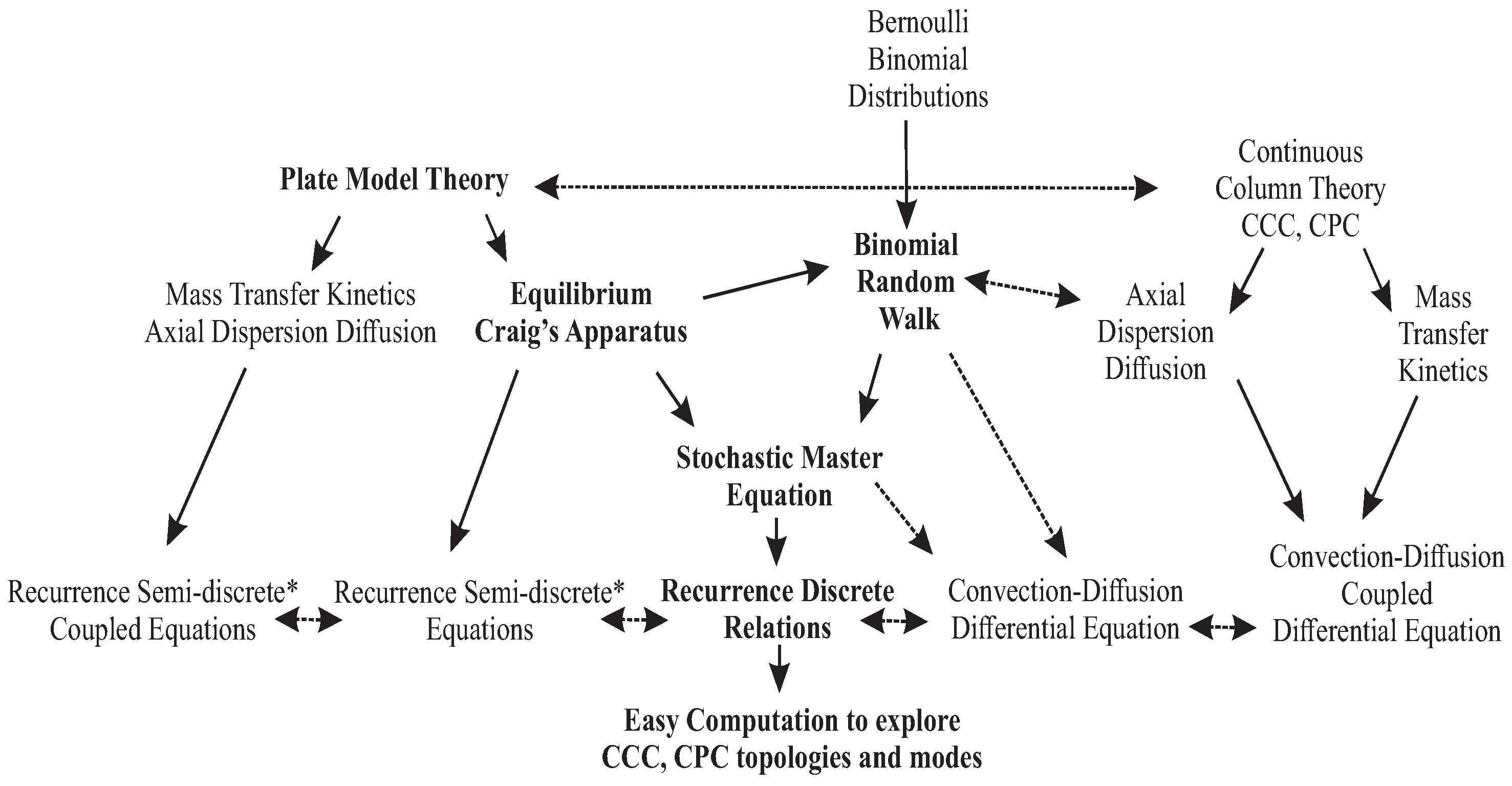
The concept of random walk was introduced as the simplest molecular chromatographic model [6,7], and it will be carefully examined to validate the recurrence principle, finding the coincidence with the stochastic master equation [8,9]. It will be compared to the continuous and discrete-continuous models to foster the coherence of the whole. In the flowchart below (Figure 1), the links are displayed between the plate model theory and the liquid–liquid reference models, already developed by several authors through the years [6,10,11,12,13,14,15].
2. Materials and Methods
2.1. The Modeling of the Craig’s Apparatus, a Precursor in Partition Chromatography
Craig’s apparatus is a former discrete prototype for partition chromatography that helps to approach the principle of more modern instruments with continuous elution, as CCC or CPC—even if, in the latter cases, partition equilibrium is not necessarily achieved when passing to the neighbouring cell.
2.1.1. The System
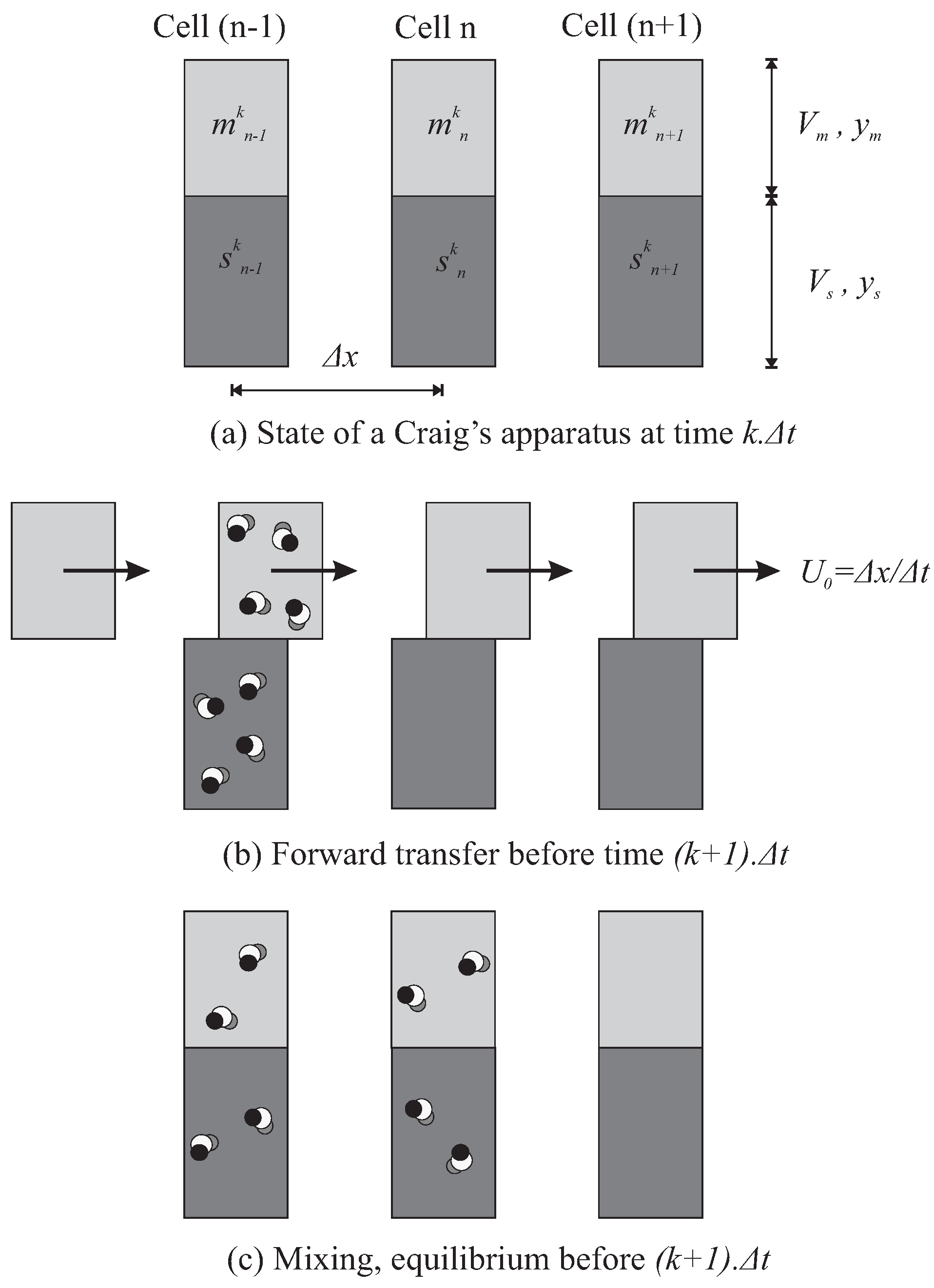
A number of identical cells (or funnels, or tubes) are assembled in series, assigned as a total as number of plates N, at constant space interval . Their individual volume is invariably partitioned between a mobile phase (MP) with volume and an immiscible stationary phase (SP) with volume (Figure 2). The cell n contains a solute at the concentrations and , for MP and SP, respectively, and where k counts constant time intervals . The principle is to inject and elute a complex sample, by mixing all the cells and then shifting every mobile phase volume of a cell to its next neighbour.
2.1.2. The Recurrence Phenomenological Model with Concentration
The model that we are going to develop is phenomenological. It fully encodes the principles implemented in the process, in terms of concentration.
We assume that the partition coefficient of the solute does not depend on concentration and that, at each transfer, the thermodynamic equilibrium is reached satisfying the condition
The Recurrence Relation
The most significant initial condition is when only the first cell is loaded with a solute. The process then consists, at each instant k, in simultaneously transferring the volume of all the cells, i.e., generally from the cell to the next n, which leads to the mass balance
All the cells are then stirred until equilibrium, which amounts to recalculating the concentrations according to (1) and to arriving at the recurrence relation
This computation highlights the combination of volumes, times the number of cells N that defines the total retention volume .
The Recurrence Relation Approximated by a Time Derivative
Van Deemter et al. introduced this recurrence computation early; however, he used the infinitesimal approximation for the time interval , with the aim of an analytical solving [6]. Nevertheless, if this formal solving expresses a didactic point of view and offers a “turn key” solution, they lack flexibility when the technical configuration becomes more complex. They require a non-negligible effort, on a case-by-case basis, without any guarantee of success a priori.
2.1.3. The Binomial Phenomenological Model in a Fraction of Injected Quantity
A phenomenological approach by recurrence was experienced also to represent in each cell the fraction of the injected quantity over time [1]. This approach is based on the consideration of the initial fractions in thermodynamic equilibrium and , in MP and SP, in the first cell. The condition is usually assumed.
The partition coefficient takes the form
This iteration develops a binomial distribution. After k transfers, the fraction in the cell n is
2.2. The Binomial Random Walk Model
Naturally, the Craig’s process obeys the case of a binomial random walk perfectly. The idea was hinted from Gidding and Eyring [23] as a random migration, and later was presented by Felinger [7].
The most simple explanation of a random walk of a solute is based on the statistical model of a coin flip, with bias: the probability p to have “heads” is between 0 and 1. The resulting distribution is binomial when evaluating the chance of having n “heads” on k trials.
When the individual draw generates a one-dimensional displacement, it is a binomial random walk. The walk can be symmetrical: on “tails,” one makes a jump to the left and on “heads” a jump to the right.
Thus, the Craig’s model fulfills the conditions. The walk is the macroscopic shift to the right of the volume . The random character comes from the chance for the solute molecule to be in MP, thus to move to the next right cell. If it is in SP, it stays in the same cell. This is actually an asymmetric random walk.
This chance depends on the Brownian motion in the two phases that can tend to a rather determined behavior when is relevant. Nevertheless, it relates also to the probability to catch the wandering solute molecule in the volume ratio . Therefore, the probabilities p and q to be in MP and SP are statistic combinations. The fraction can be considered as the thermodynamic probability to be in MP and the probability to be transferred (and the complement in SP). The retention factor , which is the ratio of matter when is the ratio of concentration, helps to simplify these probabilities:
2.2.1. The Statistical Moments of the Random Walk
The mean displacement of the solute molecule in the series of cells (column) and its standard deviation can be expressed. The binomial distribution (5) provides the statistical moments and , in the general condition where . Equivalently, the recurrence relation (3) gives the same first and second order moments, knowing that the MP concentration is the statistical distribution along the column. The first moment is the mean displacement n, or the ”barycenter” of the concentration profile
By examining the results of the two methods, we notice that
The second moment is the variance or mean of
The variance of the injection peak at the first instant is added to the diffusive variance [24].
2.2.2. Elution Speed and Diffusion Coefficient
The present study will focus on the concept of speed instead of the concepts of flow rate or residence time. The parameters of the binomial random walk are traditionally constant: the space jump , the time period . In the Craig’s process, there is therefore a notion of intrinsic speed for the MP: . The elution speed v for the solute comes out from (8) and (9)
The variance of the movement is also expressed from an intrinsic notion, that of the diffusion coefficient: . The diffusion coefficient D of the solute is therefore
2.3. Stochastic Master Equation and Differential Convection-Diffusion Equation
Let be the probability of moving n steps right after k trials. In the case of the asymmetric walk mode that concerns us, each test gives the possibility of moving forward one step with the elementary probability p, or of staying motionless with the complementary probability . Since the decision tree is binary, there exists a recursive relation connecting the state of the result to the test with the previous one k [8,9]. The state comes either from having undergone one step further, or of remaining motionless. These previous states having a probability of the same type, we can write
This relationship is called the stochastic master equation. Since concentration is similar to probability, then
or
The recurrence relation expressed in (3), obtained by modeling the instrumental principle, perfectly fits this master equation. It is a fundamental justification for the early phenomenological treatment.
When these discrete deviations become infinitesimal, this master equation tends to the differential convection–diffusion equation for a continuous concentration versus time t and space x [7]
The binomial solution tends inevitably towards the expected derivable solution of the differential equation
2.4. Model of the Continuous Column in a Non-Equilibrium State
2.4.1. Description of the Geometry
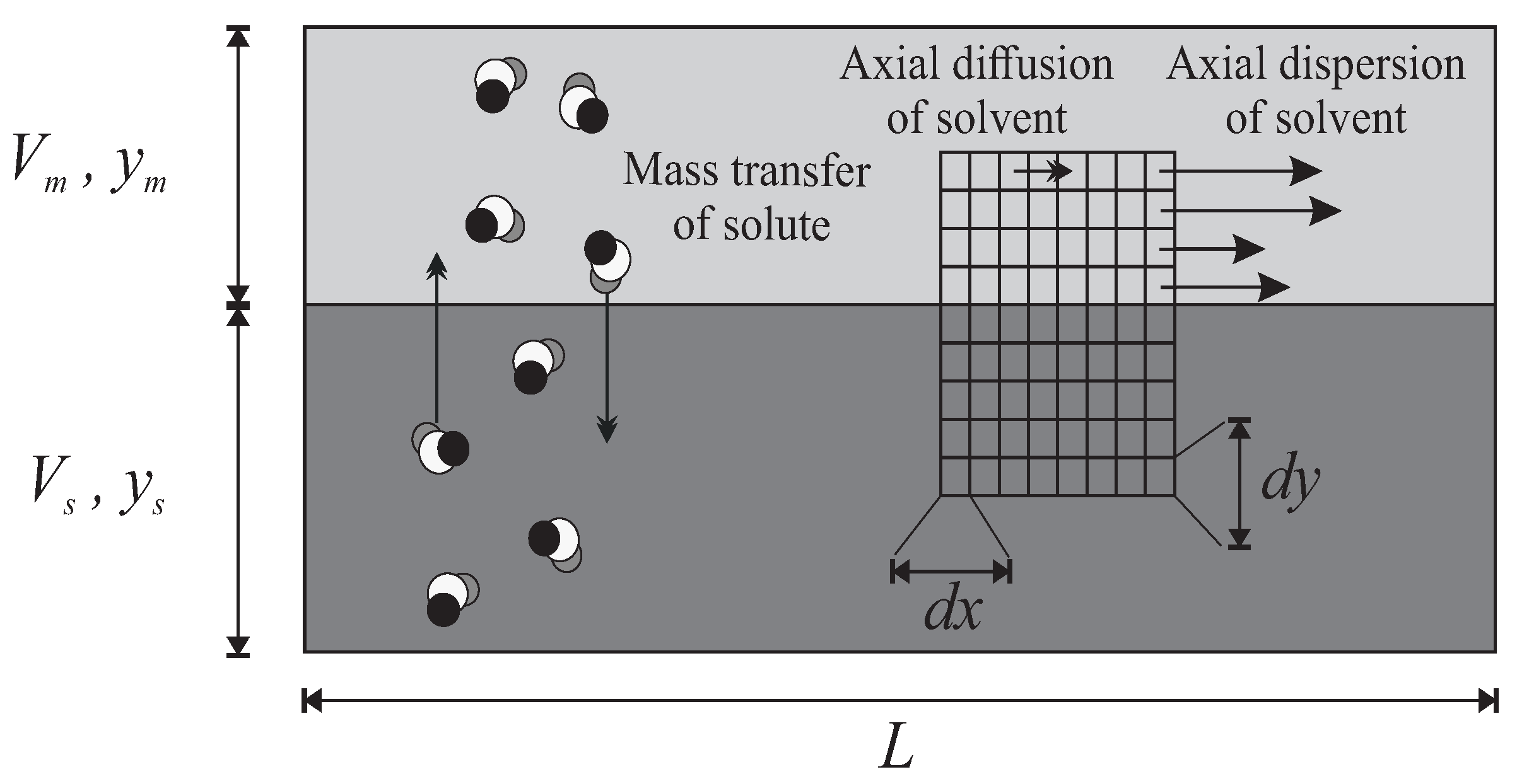
The geometry of the continuous model with axial/longitudinal dispersion is a simplified model of the real instruments (Figure 3): two continuous longitudinal media for the MP and SP, with a common interface. The MP is moving to the right with a velocity field that can undergo mainly longitudinal dispersion or even diffusion. Obviously, the solute molecules are supposed to migrate radially/transversally from one solvent to the other one and to be entrained forward by the fluctuations of MP.
This geometrical frame is not monolithic like in the geometry of the Craig’s principle. The mobile medium, for instance, can be decomposed into infinitesimal elements , according to the axes x and y, longitudinal and radial.
2.4.2. Coupled Differential Equations
The space and time variations of the concentrations, m in MP and s in SP, respectively, are derived from two coupled differential equations [11]
where is the global interfacial speed of transfer for the solute, a the specific interface area, U the speed of MP, and its retention ratio.
These equations are solved by Laplace transforms or of variable S. In terms of the characteristic transfer time , we get
2.4.3. Comparison with the Model of Craig
Limit of Null Transfer Time
In order to retrieve the Craig’s model, we can assume the extreme limit . Then, we switch back to the time domain and find an uncoupled equation for m
The agreement with the elution speed (13) is verified and in the same way the dispersion–diffusion coefficient is the ratio of according to p (14)
The conditions of motion of the mobile solvent with its own convective and diffusive parameters, U and , are adopted by the solute molecule in proportion p to its impregnation.
The question remains: if the dispersion–diffusion plays a role in the continuous model, how can one reconcile the Craig’s model that has an autonomous coefficient D?
Van Deemter et al. [6] gives the argument that we want to put forward here, if the transfer time is null or negligible compared to . The Craig’s macroscopic-microscopic and the purely microscopic continuous processes operate in a similar way, however with a different geometric partition. In the first case, the phenomenon is constrained strictly in a single unit volume, defined by the vertical extent y and horizontal width X of the cells.
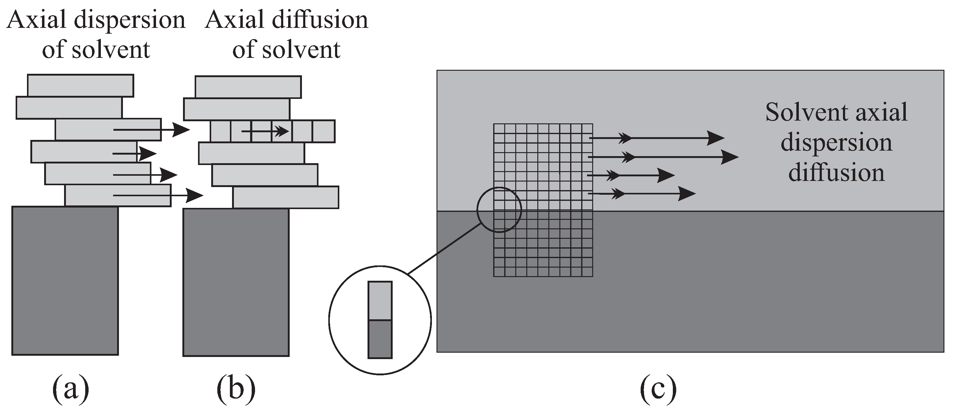
When in the continuous case the height is diced into infinitesimal intervals, or , a certain longitudinal dispersion is allowed in MP, with various horizontal progressions. The longitudinal diffusion is then revealed in the fragmentation along the x-axis, which will provide some variability in the migration (Figure 4). This diffusion comes out explicitly when the clusters of solvent transport solute molecules.
A solute molecule therefore borrows randomly “individual vehicles”, or , instead of the “synchronized bus” or the “sidewalk” . The scheme can be summarized by identifying a purely microscopic random walk of parameters p, , , , with the intrinsic dynamic characters and .
Strictly, if is exceptionally null, Equations (20) and (21) no longer work correctly. Thus, implicitly takes into account the fundamental diffusion which arises from the solute migration in the form , with a term purely dedicated to the mobile solvent “”. The usual absence of the term function of is, however, legitimate because it is very low and indeed negligible.
2.5. Plate Model Out of Equilibrium
The model of the single continuous column does not allow for detailing the particularities along the fluidic path, for a finer modeling. A better approach is to cut the geometry into sections, which will describe, for instance, several periodic patterns of a CPC instrument, with three zones of one cell and the connection duct as a particular dispersive medium [25]. For the modeling of such a “plate” i, a system of paired equations is established, for the concentrations , in MP and SP, similar to (20) and (21), but differential in time and discrete in space as in (3)
This system of equations makes it possible to manage any topologies, but also to give access to symmetrical modes, where the two phases are simultaneously put in motion in opposite directions. This concerns the dual mode of CCC and TMB of CPC [14,20,26].
In these equations, the use of an explicit diffusion term D is not essential. We know that this parameter, as in the discrete case, must emerge. On the other hand, the coefficient can be handled on purpose in the ducts connected to the cells [25].
Van Deemter et al. [6] and Kostanyan et al. [14] both show thoroughgoing and complete model representation, even though sometimes they could be relatively complex analytical solutions. Consequently, the computational process could be arduous and complicated because it would be necessary to acquire manually long expressions or for instance to solve technical problems as calculating heavy factorials.
3. Results
Three configurations of liquid–liquid chromatography will be presented. The recurrence formula will lead to concentration profiles, chromatograms, and space-time maps of concentration. The fitting with a real chromatogram will confirm the interest of the Craig’s model that plays the role of the historical plate model.
3.1. Batch Injection in Simple Elution Mode
3.1.1. Topology and Mode
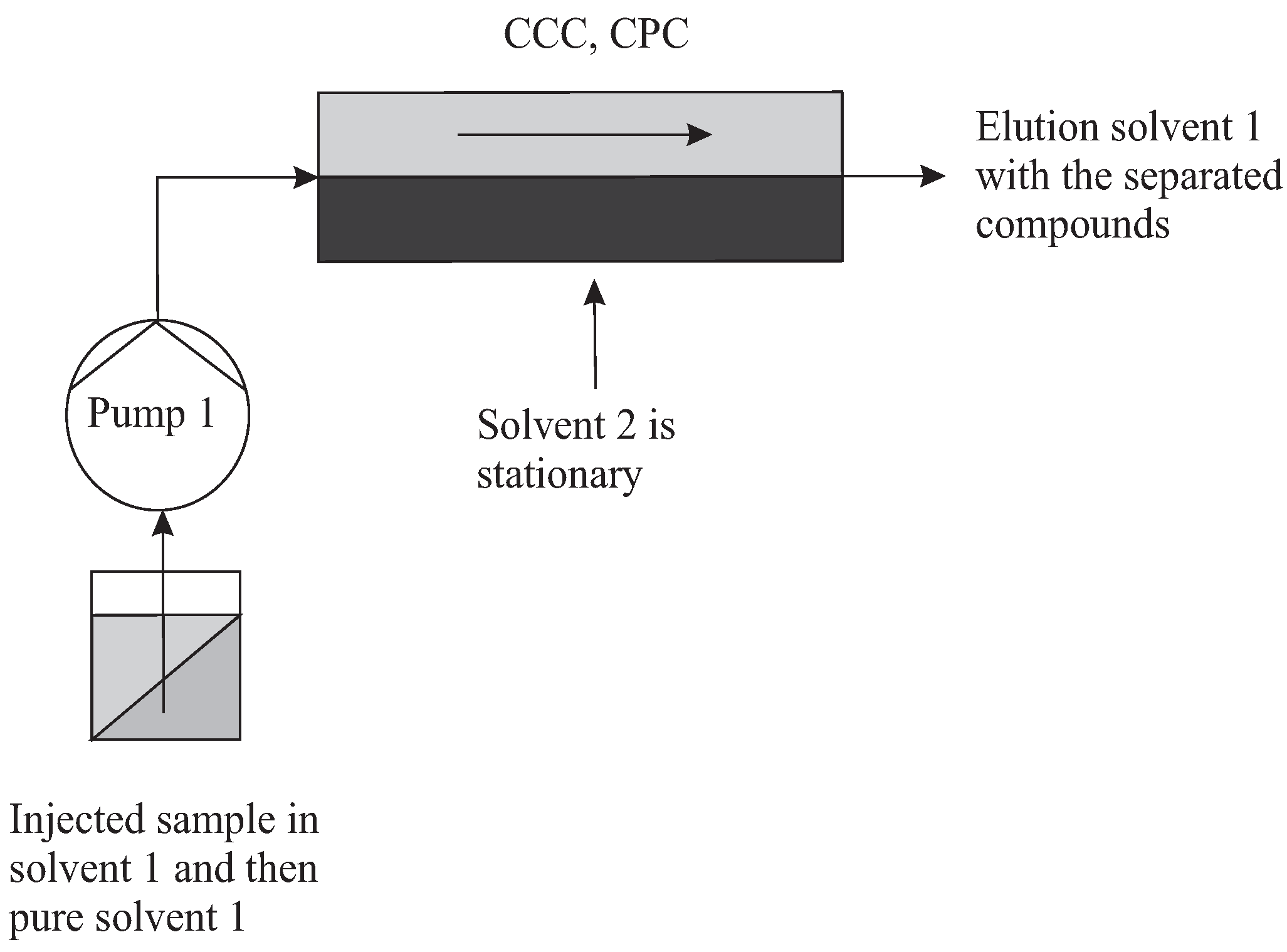
The topology needed for a batch elution is simply a column filled of SP (solvent 2), in equilibrium with MP (solvent 1). At least one pump is necessary for preparation, injection, and then elution (Figure 5). The chromatographic mode consists of injecting a certain amount of sample at the inlet in MP (solvent 1) and in eluting it until its total release.
3.1.2. System of Equations
Coding Injection
The injection determines the initial conditions of concentration in equilibrium in MP until the instant . For , the load can be equally distributed on each instant with a constant concentration:
For , there is no injection: .
Coding Elution
The SP concentrations are uncoupled and obtained by multiplying by .
3.1.3. Special Case
We compute here the case of an injection of two solutes of and , in a column of plates, with a retention ratio , an unit plate volume , an amount . Two injection times, 10 and 100 ticks, are studied.
Concentration Profiles and Chromatogram for Two Solutes
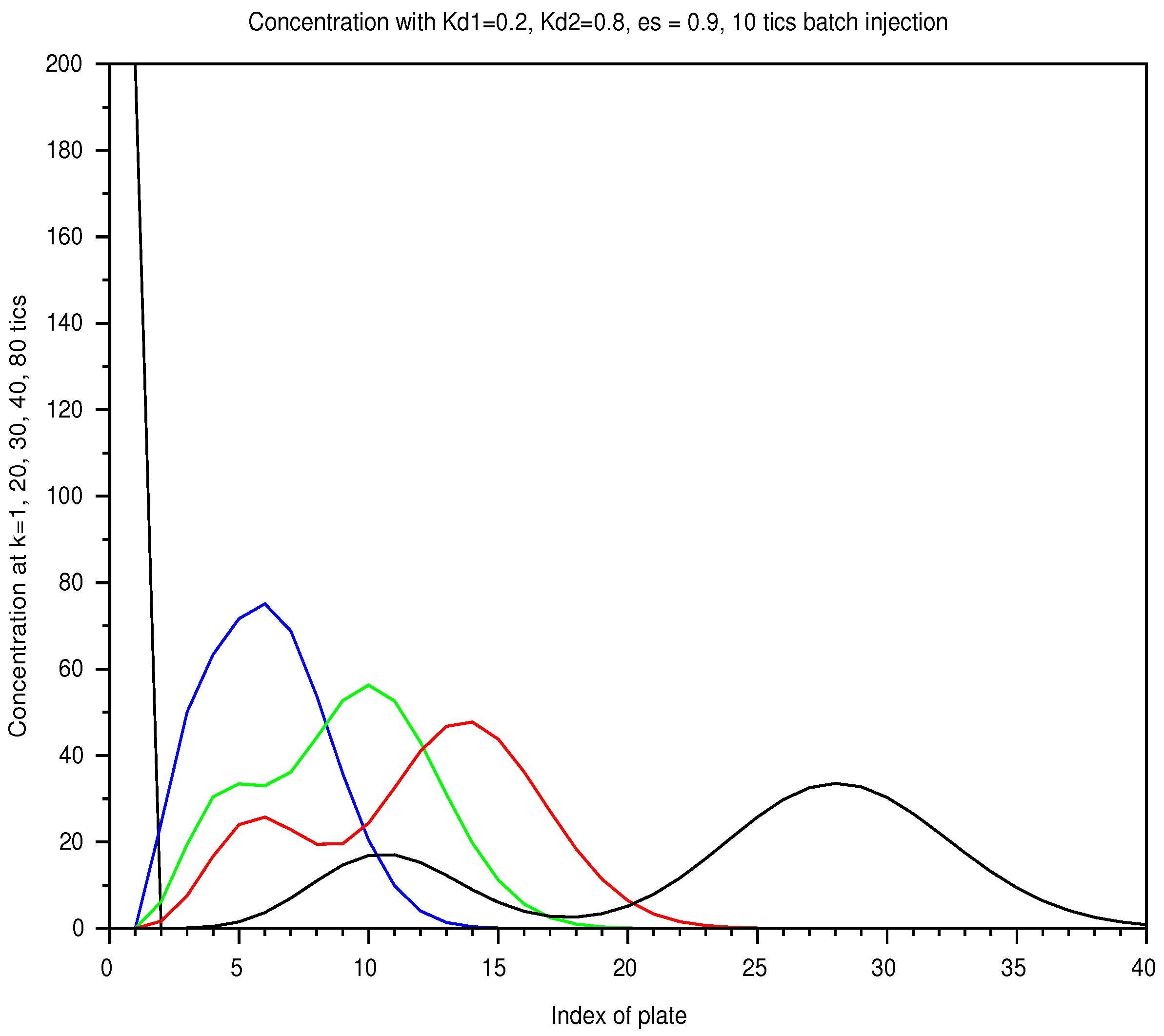
Since the injection into the plate 1, the concentration profile of each solute is supposed to evolve from a triangular shape, then trapezoidal towards a Gaussian limit that can be approximated by (19). At each moment, the barycenter of concentration, formally defined in (9), moves at constant speed v (13). The standard deviation should increase according to the typical law of diffusion: (with ).
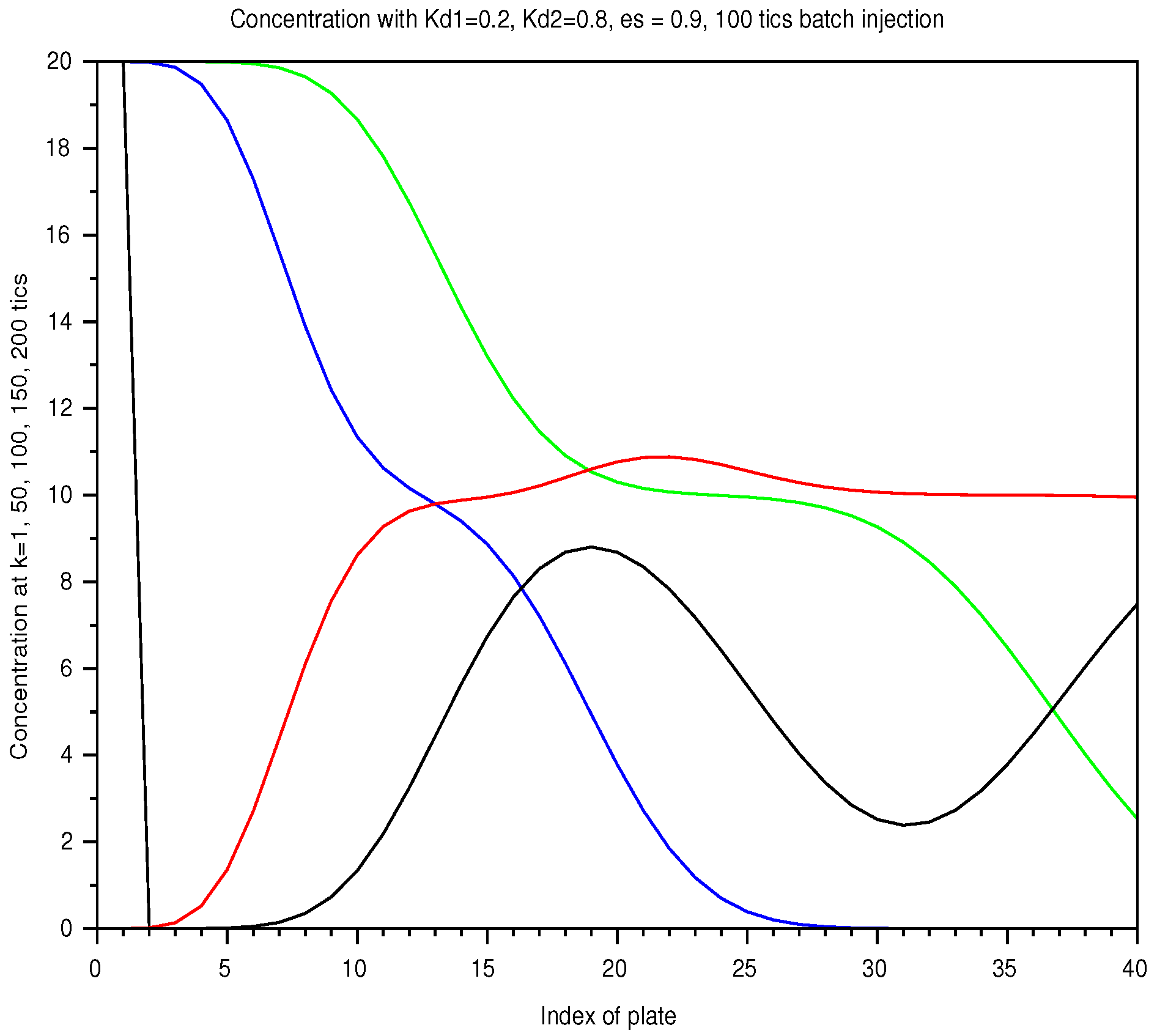
In Figure 6, we display the sum of the profiles of two solutes, injected together over the shortest period, at successive instants. Separation occurs with the speed difference but the profile spread out. In Figure 7, for the longest injection, the total separation is not reached even later, with the same injected amount.
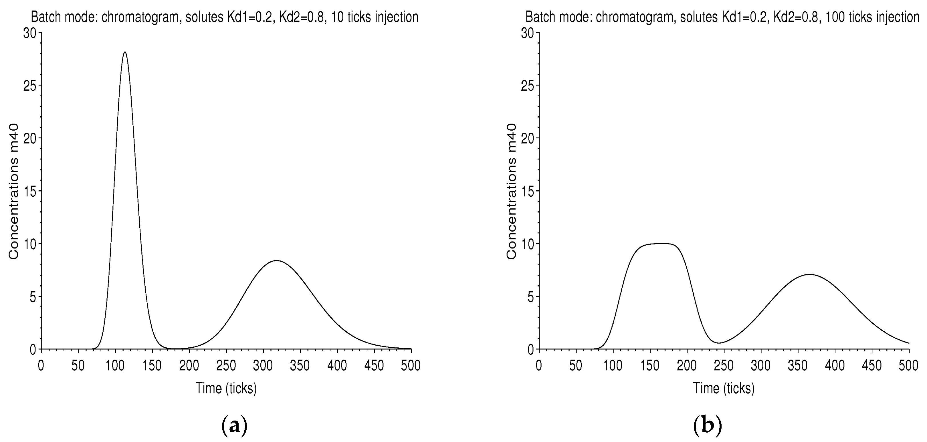
The chromatograms are displayed in Figure 8. In the case of long injection, the first one is rather square, which is the trace of the large rectangular injection smoothed by diffusion.
Space-Time Maps
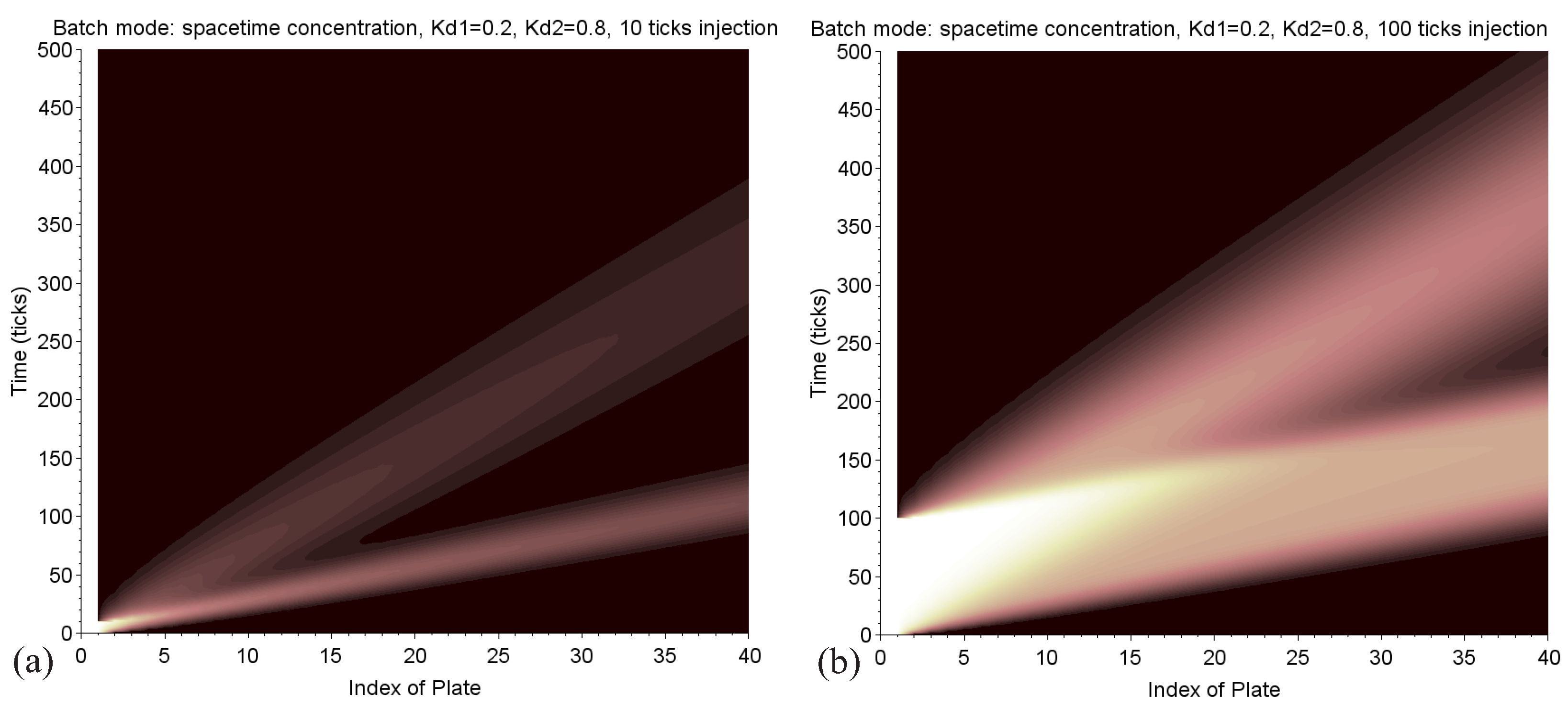
Each trajectory is therefore a straight line in a space-time graph, with a slope all the weaker as this speed is high. The advantage of the model presented here is the capability to generate this synthetic graph, representing in a single image the matrix of concentration (Figure 9). This very visual tool can help to develop a separation strategy. Maps can be easily compared within different conditions depending on the mobile phase ratio , the characteristics of injection, and the number of plates. We can see where and when the peaks separate.
3.1.4. Correspondence with a Real Chromatogram
The plate theory can make a computed chromatogram coincide with that resulting from a continuous process because they have in common the concept of random walk. For the same , the retention time in ticks and the real time, expunged of all accessory volumes, allow a time conversion to be established. The two chromatograms can be superimposed. We can then vary the number of plates N so as to obtain a width equivalent to that of the chromatogram. This number is by definition the effective number of plates for the isolated substance.
The variation of N must be done by keeping constant: the column volume , its length L, the flow F, the rate , the speed of MP, the quantity of material injected, and the duration of injection. In this context, the parameters of the discrete process are constrained:
The coefficient of intrinsic diffusion is inversely proportional to N:
We can see again that, when N is high, is negligible, which can be expected in an ideal continuous column.
Incidentally, an amplitude adjustment to accommodate the molar extinction coefficients and an offset for the baseline of the actual chromatogram will be necessary.
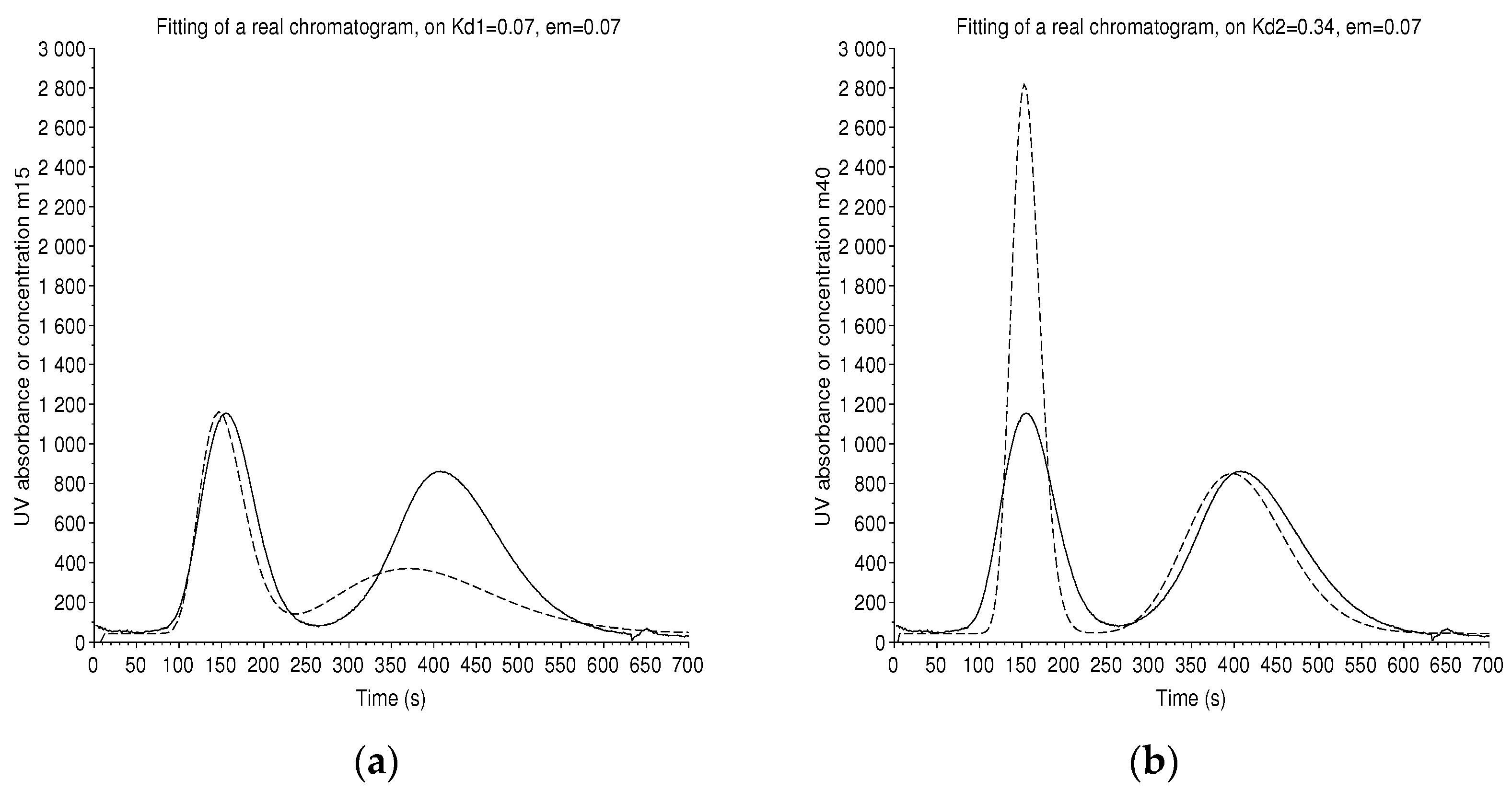
A special case is studied with a 250 mL, 240 cells CPC instrument that elutes two standards at low concentration, hydroquinone of and pyrocathecol of , with the Arizona N solvent system (heptane/ethyl acetate/methanol/water (1/1/1/1)). The conditions are: an effective volume = 210 mL, a flow rate F = 12 mL/min, with a measured retention ratio .
Each compound has its own number of theoretical plates. Thus, two different adjustments are performed (Figure 10). The plate model gives and .
Independently, we have superimposed a formal solution of the coupled Equations (20) and (21) with the criterion of the least square and found and , with the arbitrary hypothesis that . By the rough manual method of the tangents, we should have and .
In the two cases, the number of plates is rather low, so even if the retention time is very well computed, the maximum of the theoretical chromatogram is not perfectly at the same location.
3.2. Batch Injection in Multiple Dual Mode (MDM)
The separating power of a chromatography column is limited by its number of plates. Fortunately, some solutions exist, by valves sequencing, to artificially improve it [27,28,29]. We can slow down the process in the column, by a back and forth movement of “shuttle,” which will allow the separation to naturally increase: this is what the dual mode does. The dual mode highlights the advantage to have a lack of solid support and operates an inversion in elution, using the “stationary” as a “mobile” phase.
The multiple dual mode (MDM) is at least a dual mode repeated several times. The multiple inversions are time consuming but hedge the problem of poor selectivity that is often encountered in a complex mixture to separate and when the retention ratio of MP is not ideal.
3.2.1. Topology and Mode
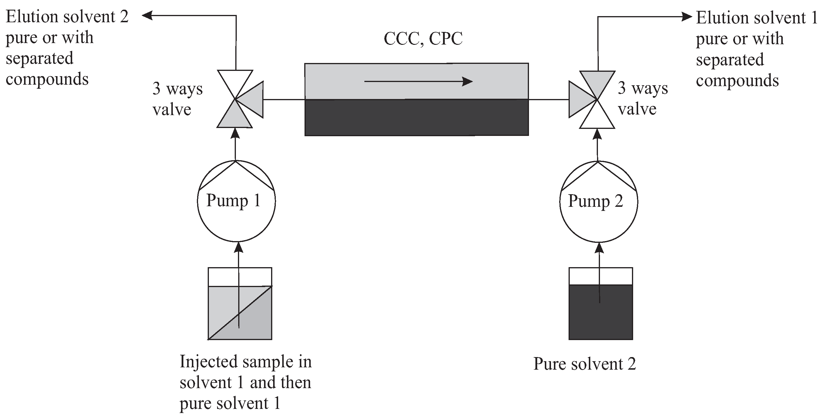
It is therefore necessary to have two three-way valves at the inlet and at the outlet which simultaneously select one or the other solvent as mobile. A second pump 2 is then devoted to the solvent 2 that was stationary (Figure 11). Once injected, in batch mode, the solutes are eluted by alternation. At the end of these cycles, the last one can be extended to complete the elution on the opposite side of that of injection. We’ll compute this case, but several other configurations are possible.
3.2.2. System of Equations
Let be the instants when the solvents switch. We therefore proceed to the following system or recurrence relations. The notation relates to solvent 1 and to solvent 2.
Coding Injection
For :
For , .
Coding the First Forward Elution
For each , we compute by incrementing n from 2 to N, to represent the forward elution:
It is now necessary to take care of obtained by multiplication by to feed the reverse computation, even for .
Coding the First Backward Elution
In the next step, the SP becomes mobile. Thus, for each , we compute by decrementing n from to 1, for a backward elution:
The concentration is prepared also for the next forward phase. The condition is imposed during this backward phase because pure solvent 2 is now pumped in.
Coding J Dual Cycles
This is the first cycle corresponding to the dual mode, with . Multiple dual mode can be developed for J cycles, by running new forward and backward elutions, each time with the respective condition and .
Coding a Final Forward Elution
At the end of these cycles, a final forward step is computed to collect the solutes. Thus, for each , we reuse the first iterations (33), until the final instant . The chromatogram is obtained by .
3.2.3. A Typical Case of Amplified Separation
Because of these alternations, the retention ratio of MP in CPC can hardly be low in search of a more resolutive separation. It will probably find a balance for . This loss of performance is, however, very quickly compensated for by the efficiency of the mode. In addition, in essence, MDM is a solution for those processes that have difficulty with finding a low MP ratio.
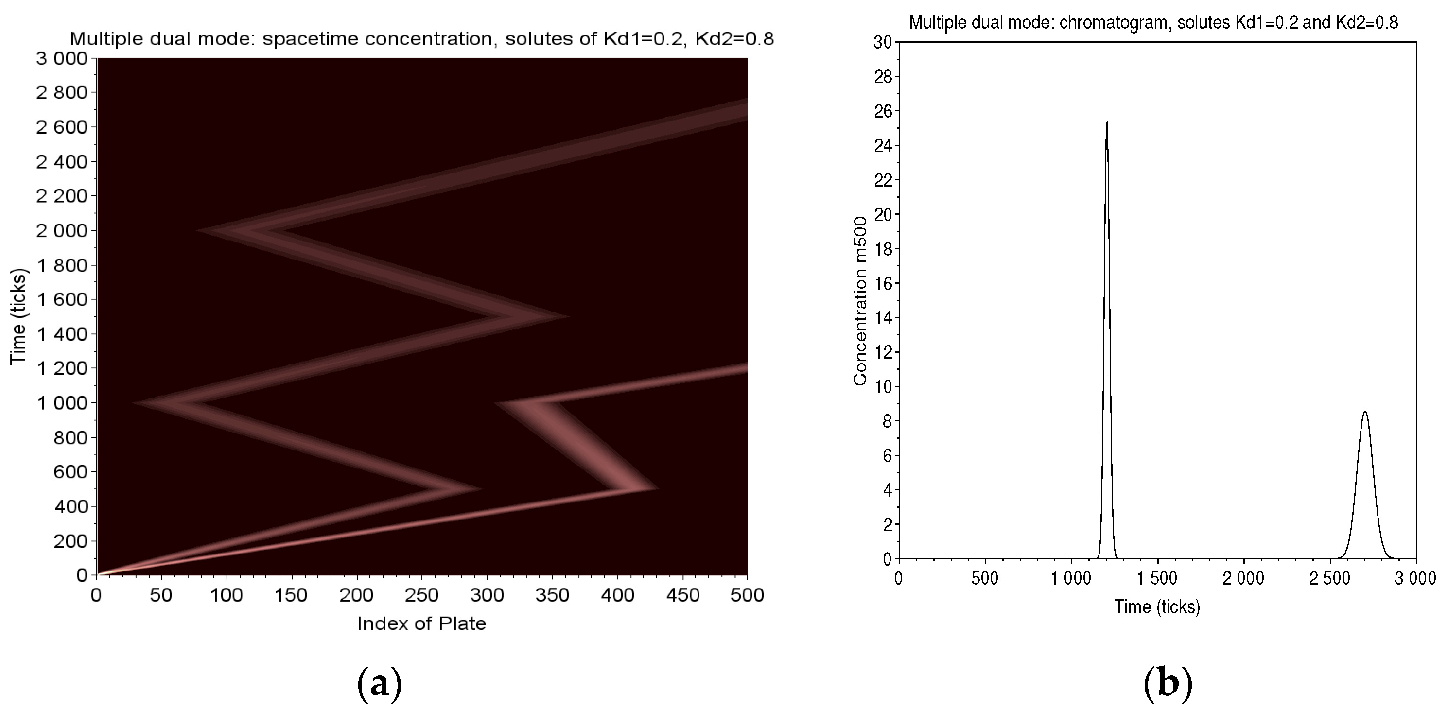
Two solutes of and are eluted in a column of 500 plates. The conditions are , and a 10-tick long injection. They are pushed forward during 500 ticks, then backward 500 ticks. In the next forward progress, the fastest solute is collected at the exit of the column. We go on one cycle more for the slower solute and finally elute it to the exit. The map of (Figure 12) clearly shows the amplifying effect of the separation in multiple dual mode.
By way of comparison, the trajectories of the two solutes are extended, if they were to be conventionally eluted on the same column. In this case, the time difference is 250 ticks. Thanks to the long sojourn of the slow solute and the fast output of the other, this difference becomes 1500 ticks, magnified by 6. The chromatogram (Figure 12) shows a first peak which is very narrow because it elutes quickly and a second very much wider (to be compared with the relative widths of a direct elution of the same solutions (right of Figure 8).
3.3. Continuous Injection in “True Moving Bed” Mode
We just studied two cases of batch injection continuously eluted—one time in simple mode, several times in opposite alternations in MDM. The next emblematic configuration will authorize a continuous central injection, synchronously with the same principle of solvent alternation through the two opposite ends of the column. The concept was patented [21] and identified as “TMB” as a response to the wish of seeing the bed of silica mobile. It was done before in the solid–liquid case, by the Simulated Moving Bed (SMB) devices, thanks to the principle of relativity of speed by reference to injection. Afterwards, a similar concept was applied, using two hydrodynamic liquid–liquid CCC columns [30,31].
3.3.1. Topology and Mode
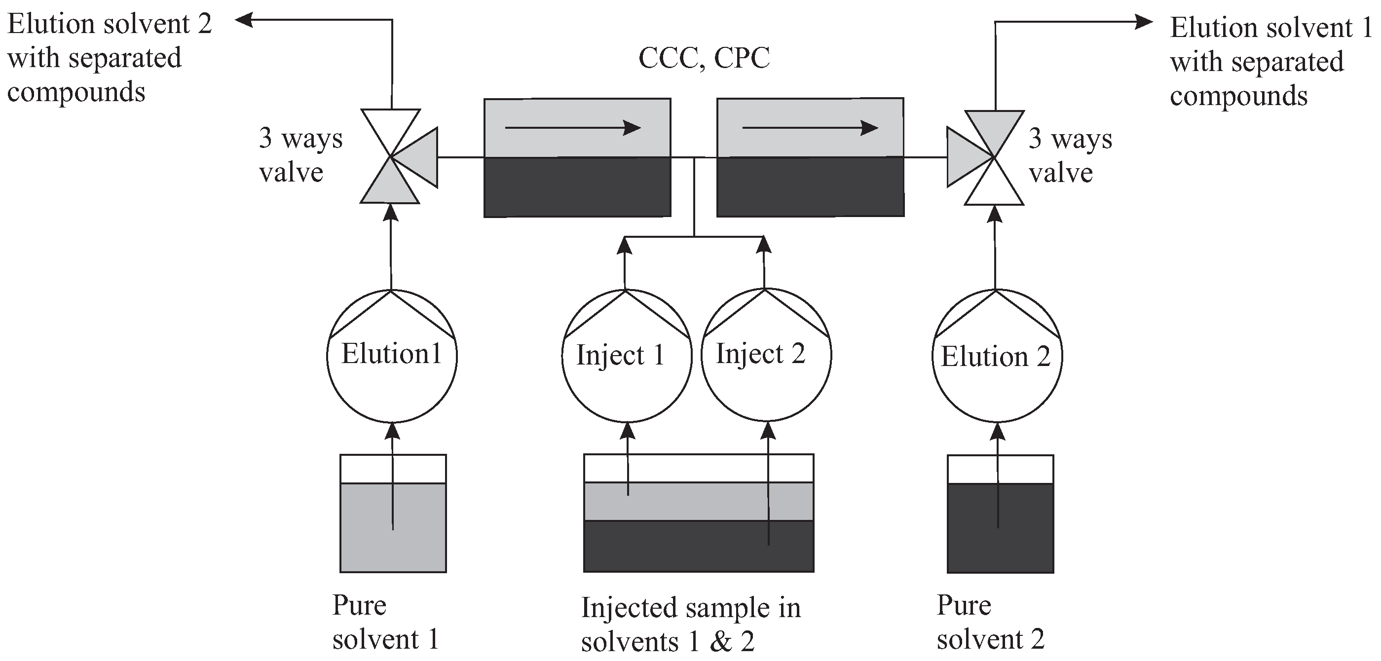
The topology which corresponds to the TMB mode is close to that of MDM, but differs by the injection terminal at the center of the column (Figure 13). We can have practically two identical columns connected in series. An additional pumping system is required for injection. The injection pump 1 introduces the sample at equilibrium in solvent 1, in conjunction with the elution pump 1, towards the right end of the column (and vice versa). By this process, the solutes of will be eluted to the right and those of to the left. In the simplest principle, the injection flow rate is negligible.
3.3.2. System of Equations
We re-use the recurrence equations of MDM, for forward and backward elution (33) and (34). being again the switching times of the solvents, but with and T the dimensionless period of alternation. The number of cycles is indicated by J.
Apart from the batch injection in MDM, the initial conditions at the inlet and outlet of the column are identical: if i is odd, or if i is even.
The specificity of this mode is to provide a different equation for the cell in the middle, of index . Thus, in the incrementation cycle (33), we insert an equation which adds the constant injected concentration in solvent 1 , so
In the decrementation cycle (34), we insert an equation which adds the constant injected concentration in solvent 2 , so
By this way, we neglect the flow of solvent injected at the same time with the solutes. We are restricted here to the essential principle, but the model can be sophisticated.
3.3.3. Special Case
We adopt the values and , , , , and .
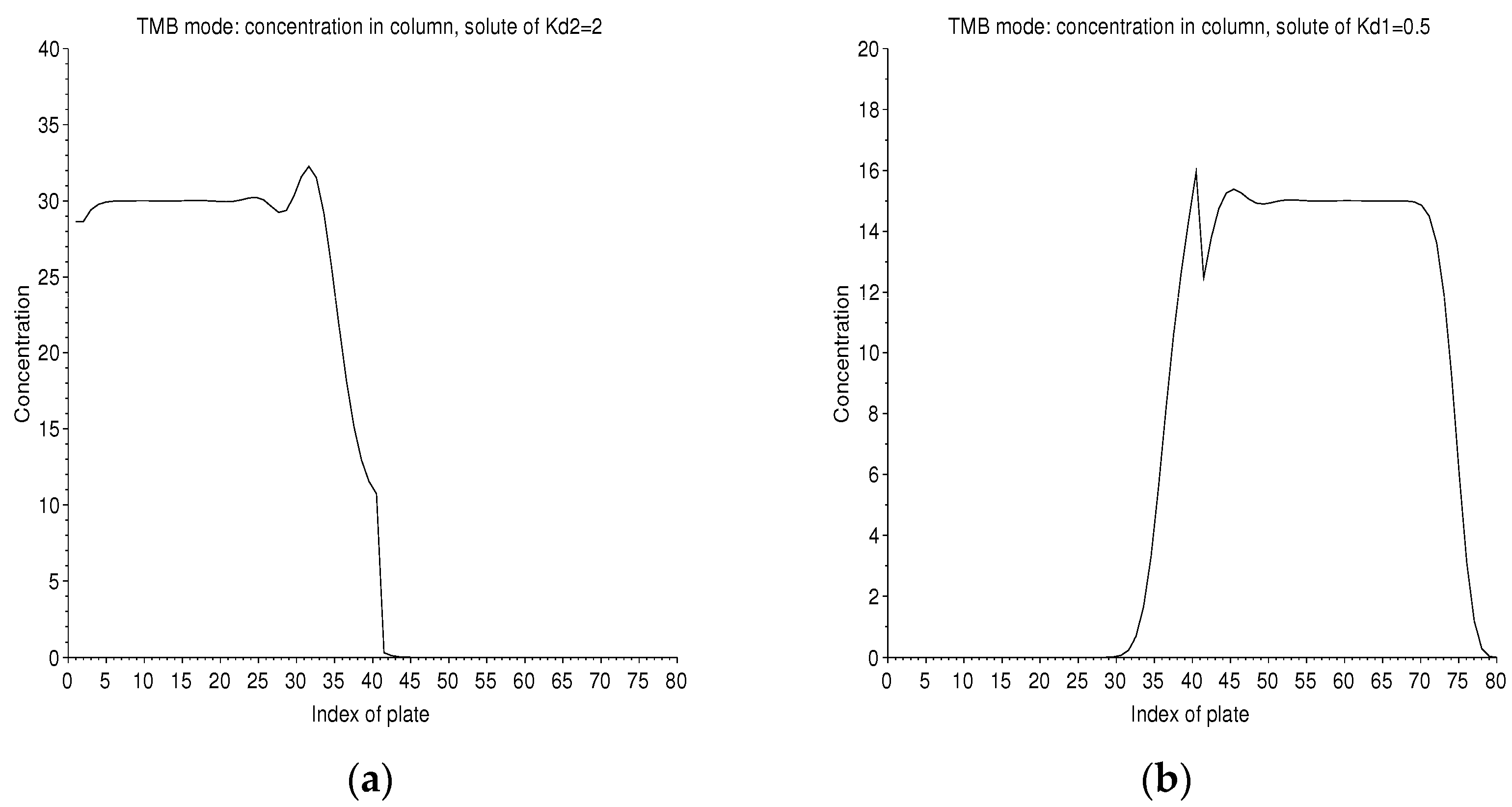
It is possible to follow the time evolution in the column for these two solutes of symmetrical with respect to 1 (Figure 14). Therefore, they will have equal and opposite migration speeds. In the steady state, the concentration profiles in the right column and the left column are flat, except at the point of injection where the feed peak is diffused on either side.
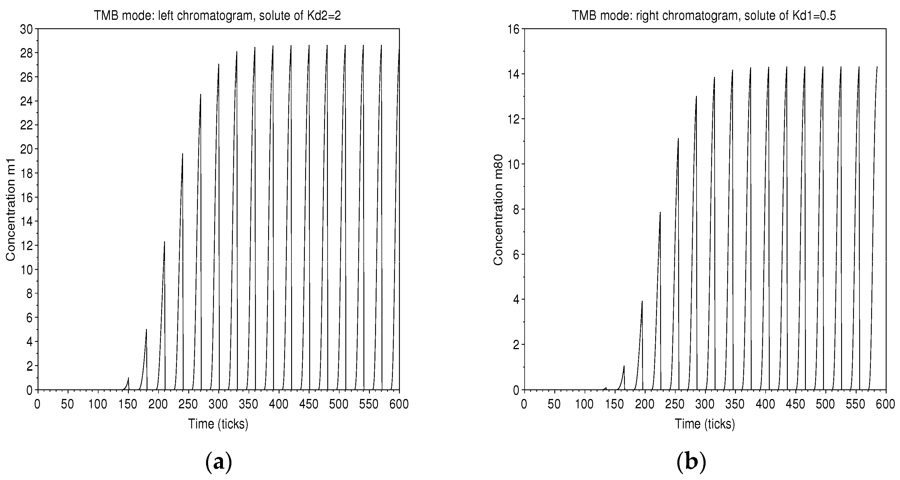
The alternating arrival of pure solvents cancels out the concentration at one end, while at the other the concentration is maximum for the collection of the solute. Accordingly, the chromatograms show output in bunches according to the period of alternation (Figure 15).
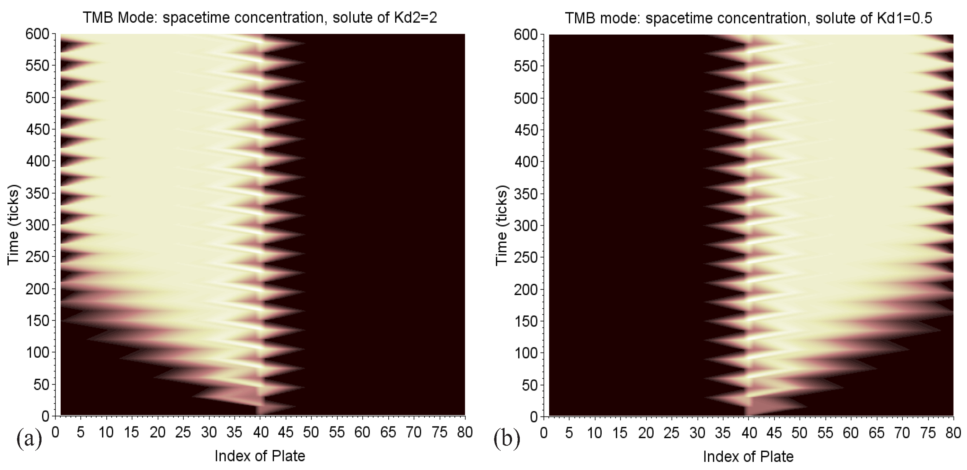
The maps in Figure 16 provide a nice illustration of what is a diffusion process with the shades of color like that of ink stains on wet paper. It also shows that the two columns are well leveraged.
4. Conclusions
Finally, the benefits of the solution by discrete recurrence could be summarized on several advantages. First and foremost, there is no need for sophisticated digital computations and we could have an exact solution of Craig’s model. This approach of liquid–liquid chromatography is then rather a translation of the problem by a feasible assembly with displacements of plates, for any topology or mode. Furthermore, the mathematical technique can lead us a step further by the simultaneous treatment of several solutes, assuming their number of plates, to assess selectivity, purity, and productivity. It makes it possible to compare, for instance, MDM to TMB and find the optimum configuration for production. Otherwise, the involvement of the nonlinear effects due to saturation solubility is rather easy to envision: the partition coefficient is modifiable with concentrations. The combination of solvent flow rates can also be computed in detail at each displacement, like in TMB mode where injection and elution meet or when the stationary phase leaks, decreasing selectivity. At the end, the method proposed in the current work is mainly dedicated to the chemistry lab staff during the process development. Implemented in Python, Matlab, Scilab, OpenBasic, Pascal, amongst others, it does not assume particular sophisticated skills. The purpose is to save time and solvents, keeping the reproducibility and the efficiency of the separation process.
Author Contributions
Conceptualization, F.D.; methodology, F.D.; software, F.D.; investigation, F.D. and T.M.; resources, T.M. and F.D.; writing—original draft preparation, F.D.; writing—review and editing, T.M. and F.D.; All the graphs and figures are made and drawn by the authors, to support the information in the paper, and they are all owned by the authors and can not be used without authorization. All authors have read and agreed to the published version of the manuscript.
Funding
This research received no external funding.
Institutional Review Board Statement
Not applicable.
Informed Consent Statement
Not applicable.
Data Availability Statement
Not applicable.
Conflicts of Interest
The authors declare no conflict of interest.
Abbreviations
The following abbreviations are used in this manuscript:
| a | Specific interfacial area (per unit volume) |
| c | Celerity of solvents in dual or TMB modes or celerity of light |
| Concentration profile for a chromatogram | |
| CCC | Counter-Current Chromatography |
| CPC | Centrifugal Partition Chromatography |
| Displacement of a solute molecule after k instants | |
| D | Diffusion coefficient for the solute in the plate theory |
| Dispersion–diffusion coefficient for the mobile solvent | |
| Diffusion coefficient in mobile phase for the solute | |
| Diffusion coefficient in stationary phase for the solute | |
| Intrinsic diffusion coefficient of random walk, i.e., of mobile phase | |
| Time step for the plate model or Craig’s apparatus | |
| x | Space step for the plate model or Craig’s apparatus |
| Ratio of mobile phase | |
| Ratio of stationary phase | |
| F | Flow rate of mobile phase |
| k | Index of time |
| Retention factor of a solute | |
| Global speed of transfer of a solute | |
| Speed of transfer of a solute in the mobile phase | |
| Speed of transfer of a solute in the stationary phase | |
| Partition coefficient of a solute | |
| L | Notion of length of column |
| m | Concentration of mobile phase without index |
| Concentration of mobile phase in cell n and at instant k | |
| MDM | Multiple dual mode |
| MP | Mobile phase |
| fraction of solute in a cell or plate | |
| n | Current index of cell or plate |
| N | Total number of cells or plates |
| p | Probability for a solute molecule to be in mobile phase due to volume selection and partition |
| Probability for a solute molecule to be in mobile phase due to partition | |
| q | Probability for a solute molecule to be in stationary phase due to volume selection and partition |
| Amount of injected solute | |
| Concentration in mobile phase in the continuous case for a solute | |
| s | Concentration of stationary phase without index |
| Concentration of stationary phase in cell n and at instant k | |
| Standard deviation of the displacement of a solute molecule after k instants | |
| SP | Stationary phase |
| U | Speed of convection |
| Intrinsic speed of random walk, i.e of mobile phase | |
| T | Duration of a TMB cycle |
| TMB | True Moving Bed |
| Volume of one cell or plate | |
| Total volume of a column | |
| Volume of mobile phase of one cell or plate | |
| Volume of stationary phase of one cell or plate | |
| Total retention volume for a solute | |
| x | Horizontal space axis |
| X | Width of a cell or plate |
| y | Vertical space axis |
References
- Martin, A.J.; Synge, R.L. A new form of chromatogram employing two liquid phases: A theory of chromatography. 2. Application to the micro-determination of the higher monoamino-acids in proteins. Biochem. J. 1941, 35, 1358–1368. [Google Scholar] [CrossRef]
- Snyder, L.R.; Kirkland, J.J.; Dolan, J.W. Introduction to Modern Liquid Chromatography, 3rd ed.; John Wiley & Sons, Inc.: Hoboken, NJ, USA, 2010. [Google Scholar]
- Craig, L. Identification of small amounts of organic compounds by distribution studies II. Separation by counter-current distribution. J. Biol. Chem. 1944, 155, 519–534. [Google Scholar] [CrossRef]
- Snyder, L.; Cox, G.; Antle, P. Preparative separation of peptide and protein samples by High-performance liquid chromatography with gradient elution I. The Craig model as a basis for computer simulations. J. Chromatogr. 1988, 444, 303–325. [Google Scholar] [CrossRef]
- Conway, W.; Petroski, R. Modern Countercurrent Chromatography; American Chemical Society: Washington, DC, USA, 1995. [Google Scholar]
- Van Deemter, J.; Zuiderweg, F.; Klinkenberg, A.V. Longitudinal diffusion and resistance to mass transfer as causes of nonideality in chromatography. Chem. Eng. Sci. 1956, 5, 271–289. [Google Scholar] [CrossRef]
- Felinger, A. Data Analysis and Signal Processing in Chromatography; Elsevier: Amsterdam, The Netherlands, 1998. [Google Scholar]
- Nauman, E. Residence time distributions in systems governed by the dispersion equation. Chem. Eng. Sci. 1981, 36, 957–966. [Google Scholar] [CrossRef]
- Vatistas, N. Danckwerts’ degree of segregation for the axial dispersion model. Chem. Eng. Sci. 1991, 46, 307–311. [Google Scholar] [CrossRef]
- Van Buel, M.; Van der Wielen, L.; Luyben, K.C.A. Effluent concentration profiles in centrifugal partition chromatography. AIChE J. 1997, 43, 693–702. [Google Scholar] [CrossRef]
- Marchal, L. Contribution à la Théorie et au Développement de la Chromatographie de Partage Centrifuge: Etude de l’Hydrodynamique des Phases et du Transfert de Matière. Ph.D. Thesis, University of Nantes, Nantes, France, 2001. [Google Scholar]
- Marchal, L.; Legrand, J.; Foucault, A. Mass transport and flow regimes in centrifugal partition chromatography. AIChE J. 2002, 48, 1692–1704. [Google Scholar] [CrossRef]
- Adelmann, S.; Baldhoff, T.; Koepcke, B.; Schembecker, G. Selection of operating parameters on the basis of hydrodynamics in centrifugal partition chromatography for the purification of nybomycin derivatives. J. Chromatogr. A 2013, 1274, 54–64. [Google Scholar] [CrossRef]
- Kostanyan, A.E.; Belova, V.V.; Kholkin, A.I. Modeling counter-current and dual counter-current chromatography using longitudinal mixing cell and eluting counter-current distribution models. J. Chromatogr. A 2007, 1151, 142–147. [Google Scholar] [CrossRef]
- Morley, R.; Minceva, M. Trapping multiple dual mode centrifugal partition chromatography for the separation of intermediately-eluting components: Throughput maximization strategy. J. Chromatogr. A 2017, 1501, 26–38. [Google Scholar] [CrossRef] [PubMed]
- Rubio, N.; Ignatova, S.; Minguillón, C.; Sutherland, I.A. Multiple dual-mode countercurrent chromatography applied to chiral separations using a (S)-naproxen derivative as chiral selector. J. Chromatogr. A 2009, 1216, 8505–8511. [Google Scholar] [CrossRef] [PubMed]
- Mekaoui, N.; Berthod, A. Using the liquid nature of the stationary phase. VI. Theoretical study of multi-dual mode countercurrent chromatography. J. Chromatogr. A 2011, 1218, 6061–6071. [Google Scholar] [CrossRef]
- Mekaoui, N.; Berthod, A. Application du dual-mode multiple aux séparations chirales en chromatographie à contre courant. In Proceedings of the SEP 2011–9ème Congrès Francophone de l’AFSep sur les Sciences Séparatives et les Couplages, Toulouse, France, 23–25 March 2011. [Google Scholar]
- Kostanyan, A.E.; Erastov, A.A.; Shishilov, O.N. Multiple dual mode counter-current chromatography with variable duration of alternating phase elution steps. J. Chromatogr. A 2014, 1347, 87–95. [Google Scholar] [CrossRef]
- Hopmann, E.; Goll, J.; Minceva, M. Sequential centrifugal partition chromatography: A new continuous chromatographic technology. Chem. Eng. Technol. 2012, 35, 72–82. [Google Scholar] [CrossRef]
- Couillard, F.; Foucault, A.; Durand, D. Method and Device for Separating Constituents of a Liquid Charge by Means of Liquid–Liquid Centrifuge Chromatography. US Patent 7,422,685, 9 September 2008. [Google Scholar]
- Rodrigues, A. Simulated Moving Bed Technology Principles, Design and Process Applications; Elsevier: Oxford, UK, 2015. [Google Scholar]
- Giddings, J.C.; Eyring, H. A molecular dynamic theory of chromatography. J. Phys. Chem. 2002, 59, 416–421. [Google Scholar] [CrossRef]
- Kostanyan, A.E. On influence of sample loading conditions on peak shape and separation efficiency in preparative isocratic counter-current chromatography. J. Chromatogr. A 2012, 1254, 71–77. [Google Scholar] [CrossRef] [PubMed]
- Schwienheer, C.; Krause, J.; Schembecker, G.; Merz, J. Modeling centrifugal partition chromatography separation behavior to characterize influencing hydrodynamic effects on separation efficiency. J. Chromatogr. A 2017, 1492, 27–40. [Google Scholar] [CrossRef]
- Ignatova, S.; Hewitson, P.; Mathews, B.; Sutherland, I. Evaluation of dual flow counter-current chromatography and intermittent counter-current extraction. J. Chromatogr. A 2011, 1218, 6102–6106. [Google Scholar] [CrossRef] [PubMed]
- Roullier, C.; Chollet-Krugler, M.; Bernard, A.; Boustie, J. Multiple dual-mode centrifugal partition chromatography as an efficient method for the purification of a mycosporine from a crude methanolic extract of Lichina pygmaea. J. Chromatogr. B 2009, 877, 2067–2073. [Google Scholar] [CrossRef] [PubMed]
- Delannay, E.; Toribio, A.; Boudesocque, L.; Nuzillard, J.M.; Zeches-Hanrot, M.; Dardennes, E.; Le Dour, G.; Sapi, J.; Renault, J.H. Multiple dual-mode centrifugal partition chromatography, a semi-continuous development mode for routine laboratory-scale purifications. J. Chromatogr. A 2006, 1127, 45–51. [Google Scholar] [CrossRef] [PubMed]
- Mandova, T.; Audo, G.; Michel, S.; Grougnet, R. Off-line coupling of new generation centrifugal partition chromatography device with preparative high pressure liquid chromatography-mass spectrometry triggering fraction collection applied to the recovery of secoiridoid glycosides from Centaurium erythraea Rafn. (Gentianaceae). J. Chromatogr. A 2017, 1513, 149–156. [Google Scholar] [PubMed]
- Mekaoui, N.; Chamieh, J.; Dugas, V.; Demesmay, C.; Berthod, A. Purification of Coomassie Brilliant Blue G-250 by multiple dual mode countercurrent chromatography. J. Chromatogr. A 2012, 1232, 134–141. [Google Scholar] [CrossRef]
- Hewitson, P.; Ignatova, S.; Haoyu, Y.; Chen, L.; Sutherland, I. Intermittent counter-current extraction as an alternative approach to purification of Chinese herbal medicine. J. Chromatogr. A 2009, 1216, 4187–4192. [Google Scholar] [CrossRef] [PubMed]
Figure 1.
Flowchart of the different modeling methods for liquid–liquid chromatography (*semi-discrete or discrete-continuous mean with a time derivative and space discrete difference). The central path (in bold) is the vein of the article.
Figure 1.
Flowchart of the different modeling methods for liquid–liquid chromatography (*semi-discrete or discrete-continuous mean with a time derivative and space discrete difference). The central path (in bold) is the vein of the article.

Figure 2.
Mechanism at work in Craig’s machine (a). Between the instant k and , all the MP volumes (light grey) are transferred to the next cell. SP volumes (dark grey) don’t move. Injection is typically performed in the first cell. Few solute molecules are represented and can be followed (b). During the same time interval, all the cells are agitated simultaneously to reach the partition equilibrium (c). The effective speed of MP results from the space interval between the cells and the time required for transfer/mixing/equilibrium that is . Then, pure MP feeds the first cell at each instant.

Figure 3.
The continuous column model with axial dispersion. A continuous volume of MP (light grey) above a volume of SP (dark grey). Solute molecules diffuse radially in both directions. The movement of the mobile solvent is also subjected to an axial dispersion–diffusion phenomenon, around a given average speed. The degrees of freedom of movement can be studied by an infinitesimal fragmentation .

Figure 4.
Extrapolation of axial dispersion (a) and diffusion (b) of MP from a re-inspired “exploded” Graig’s cell. The equivalence of the Craig’s model with the continuous model (c) is found on a two-phase infinitesimal element (in zoom).
Figure 4.
Extrapolation of axial dispersion (a) and diffusion (b) of MP from a re-inspired “exploded” Graig’s cell. The equivalence of the Craig’s model with the continuous model (c) is found on a two-phase infinitesimal element (in zoom).

Figure 5.
Simple topology of batch mode. Solvent 1 is the MP, solvent 2 is the SP.

Figure 6.
Batch mode: spatial concentration in a column of 40 plates, with a retention ratio , an unit plate volume , an amount , from a 10 tick-injection, with two solutes of and . As the elution proceeds, the two solutes spread out according to a diffusion process and are separated. The list of instants is color coded: 1 (black), 20 (blue), 30 (green), 40 (red), 80 ticks (black).

Figure 7.
Batch mode: spatial concentration in a column of 40 plates, with a retention ratio , an unit plate volume , an amount , from a 100 ticks injection, with two solutes of and . As elution proceeds, the two solutes are not totally separated in the column.The list of instants is color coded: 1 (black), 50 (blue), 100 (green), 150 (red), 200 ticks (black).

Figure 8.
Batch mode: on the left graph (a), the chromatogram measured at the outlet of the column of 40 plates is displayed, with a retention ratio , an unit plate volume , an amount . The first peak corresponds to the solute of and the next one to that of , for an injection 10 ticks long. On the right graph (b), the injection is 100 ticks long. The two peaks are larger and are not completely resolved.

Figure 9.
Batch mode: in these two figures, the space-time concentration map is displayed, where each colored point encodes the value . The lowest trace is the path of the solute of and the upper one is related to . The left picture (a) is related to a 10-tick injection, the right one (b) to 100 ticks. In the latter case, the two peaks are larger and are not completely resolved.

Figure 10.
Batch mode: a real chromatogram (solid line) with two solutes, hydroquinone and pyrocatechol in Arizona N solvent system, from a 250 mL, 240 cells CPC instrument, at a flow rate of 12 mL/min. The number of plates is not uniform from peak to peak. A simulated chromatogram (dashed line) is made to coincide on the peak of hydroquinone at (a) and on the peak of pyrocatechol at (b). We find the theoretical number of plates and . For a low number of plates, even if the retention time is well computed, the maximum of the peak is slightly shifted.

Figure 11.
Typical topology of multiple dual mode (MDM). Here, the direction of elution with solvent 1 (light grey) is represented. In the following cycle, pump 2 can put in motion the second immiscible solvent 2 (dark grey). It is assumed here in the special case that an injection is made in solvent 1 (grey) and that the collection of separated solutes is done on the right in solvent 1.

Figure 12.
Multiple Dual Mode: two solutes of and are eluted in a column of 500 plates (, with a 10 ticks long injection). There are two cycles of 500 ticks followed by a final forward elution. The map of displays the strategy adopted in MDM to improve the natural separation between two solutes (a). The long sojourn time obtained for the slowest solute magnifies by a factor of 6 the retention time between two solutes. The corresponding chromatogram (b) shows the distortion of width due to the too short sojourn time for the first peak and the long one for the second.

Figure 13.
The topology which corresponds to the TMB mode is close to that of MDM. Injections in between two columns are performed by dedicated pumps. Elution pump 1 works synchronously with injection pump 1 in the forward direction (and vice versa pump 2).
Figure 13.
The topology which corresponds to the TMB mode is close to that of MDM. Injections in between two columns are performed by dedicated pumps. Elution pump 1 works synchronously with injection pump 1 in the forward direction (and vice versa pump 2).

Figure 14.
TMB mode: concentration profiles in the two columns of 40 plates, in solvent 2 on the left (a) for and in solvent 1 on the right (b) for . This is the start of the twentieth cycle of ebb/flow. Each cycle has a duration of 15 ticks. The separation regime is established. The concentration profile is flat, except at the peak of injection into the 40 cell, which diffuses. We have just injected solvent 2 on the right end of the column, while the solute of is collected. The profile of each solute encroaches a little on the column, which is unfavorable to it.

Figure 15.
TMB mode: chromatograms of the solute of in solvent 2, on the left (a), and of the solute of in solvent 1, on the right (b). The initiation of the process and the established regime are identified. Collections can be made every 15 ticks.
Figure 15.
TMB mode: chromatograms of the solute of in solvent 2, on the left (a), and of the solute of in solvent 1, on the right (b). The initiation of the process and the established regime are identified. Collections can be made every 15 ticks.

Figure 16.
TMB mode: space-time maps of the solute concentration of in solvent 2, on the left (a), and of the solute of in solvent 1, on the right (b). The shades of color highlight the phenomenon of diffusion, like that of ink stains on wet paper. The zigzags in the center represent the alternate diffusion of the continuous injection. The incursion of each solute in the zone, which is unfavorable to it (in dark), is limited. The delivery corresponds to the clear triangles, which point to the plate 1 on the left and 80 on the right.

Publisher’s Note: MDPI stays neutral with regard to jurisdictional claims in published maps and institutional affiliations. |
© 2021 by the authors. Licensee MDPI, Basel, Switzerland. This article is an open access article distributed under the terms and conditions of the Creative Commons Attribution (CC BY) license (https://creativecommons.org/licenses/by/4.0/).
Share and Cite
MDPI and ACS Style
Dijoux, F.R.; Mandova, T. Easy Computation of the Various Topologies and Modes of Liquid–Liquid Partition Chromatography by the Theory of Random Walks. Separations 2021, 8, 41. https://doi.org/10.3390/separations8040041
AMA Style
Dijoux FR, Mandova T. Easy Computation of the Various Topologies and Modes of Liquid–Liquid Partition Chromatography by the Theory of Random Walks. Separations. 2021; 8(4):41. https://doi.org/10.3390/separations8040041
Chicago/Turabian StyleDijoux, Frédéric R., and Tsvetelina Mandova. 2021. "Easy Computation of the Various Topologies and Modes of Liquid–Liquid Partition Chromatography by the Theory of Random Walks" Separations 8, no. 4: 41. https://doi.org/10.3390/separations8040041
Note that from the first issue of 2016, this journal uses article numbers instead of page numbers. See further details here.