Automatic Detection of Individual Trees from VHR Satellite Images Using Scale-Space Methods


1
Faculty of Geo-Information Science and Earth Observation (ITC), University of Twente, 7514 AE Enschede, The Netherlands
2
CGI Nederland, 3068 AX Rotterdam, The Netherlands
3
ICEYE, 02150 Espoo, Finland
*
Author to whom correspondence should be addressed.
Sensors 2020, 20(24), 7194; https://doi.org/10.3390/s20247194
Submission received: 15 October 2020
/
Revised: 9 December 2020
/
Accepted: 10 December 2020
/
Published: 15 December 2020
(This article belongs to the Section Sensing and Imaging)
Abstract
:This research investigates the use of scale-space theory to detect individual trees in orchards from very-high resolution (VHR) satellite images. Trees are characterized by blobs, for example, bell-shaped surfaces. Their modeling requires the identification of local maxima in Gaussian scale space, whereas location of the maxima in the scale direction provides information about the tree size. A two-step procedure relates the detected blobs to tree objects in the field. First, a Gaussian blob model identifies tree crowns in Gaussian scale space. Second, an improved tree crown model modifies this model in the scale direction. The procedures are tested on the following three representative cases: an area with vitellaria trees in Mali, an orchard with walnut trees in Iran, and one case with oil palm trees in Indonesia. The results show that the refined Gaussian blob model improves upon the traditional Gaussian blob model by effectively discriminating between false and correct detections and accurately identifying size and position of trees. A comparison with existing methods shows an improvement of 10–20% in true positive detections. We conclude that the presented two-step modeling procedure of tree crowns using Gaussian scale space is useful to automatically detect individual trees from VHR satellite images for at least three representative cases.
1. Introduction
Remote sensing (RS) imagery and technologies can help scientists to detect and delineate individual trees in precision orchard management. This is important information for efficient decision making regarding crop health and crop water requirement. Trees establish a spatial pattern at both coarse and fine spatial resolutions. These patterns can be characterized by different parameters such as shape, location, species, and crown size [1]. There is a need to precisely estimate tree parameters such as tree size and biomass from an image. In the past, the relatively coarse resolution of images was inadequate to delineate tree crowns individually [2]. Such images provided insufficient spectral and geometrical detail information. In contrast, high resolution images provide the necessary detailed information, for example, allows for identifying geometrical and spectral information of adjacent tree canopy interlocks.
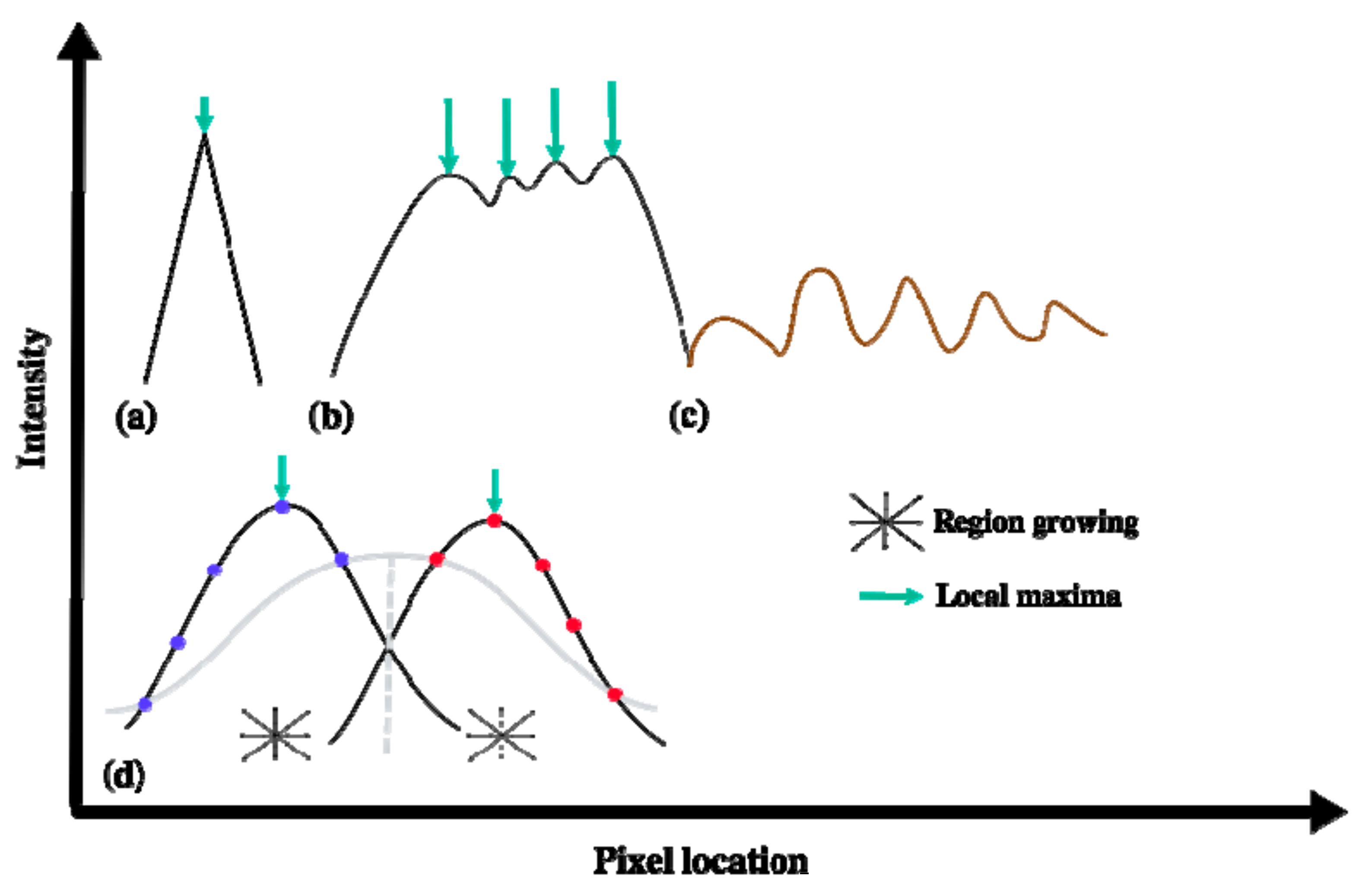
Obtaining detailed and reliable information on each individual tree from RS images requires many spectral and geometrical details. In particular, WorldView-2 imagery (WV-2) contains panchromatic and multispectral images with spatial resolution of 0.5 m (panchromatic band) and 2 m (visible and NIR bands), respectively. This resolution level is still too coarse for delineating interlocking tree crown boundaries, despite several image processing techniques that have been proposed to do so. For instance, region-based image segmentation [3] requires prior knowledge information on tree shape and size; image template matching [4,5] is useful for trees of the same height, size, and species; and watershed segmentation [6,7,8,9,10] suffers from over and under segmentation due to differences in tree heights and variation in the density of tree crowns [11]. In addition, other methods have not solved this problem. Valley following [12] explores local minima of neighboring tree crown boundaries in a way similar to edge detection [13,14,15,16,17]. The local maxima technique [18,19] searches local maxima corresponding to image brightness values at the center of the trees [15]. This technique, however, suffers from two limitations, i.e., it only detects the location of the tree and it suffers from multiple detections in irregular tree crown surfaces (Figure 1b), mainly due to the presence of multiple local maxima occurring at a single tree due to complexity in tree branches and the presence of wood or grass as background noise. To overcome the multiple local maxima problem, one can apply a fitted pre-smoothed Gaussian filter, but in the presence of adjacent tree interlocks this results in inaccurate tree sizes and imprecise locations. Figure 1 illustrates the local maxima of a coniferous tree in a natural forest area and a broad-leaved tree with several local maxima in an orchard area, where the number of local maxima depends upon spatial and spectral resolution of the sensor. The local maxima technique has been used in several studies to detect coniferous trees, but for broad-leaved trees it is inconvenient.
To overcome the multiple maxima problem of the broad-leaved trees, Ardila et al. [2] proposed a pre-smoothing Gaussian filter on a tree crown, followed by fitting a two-dimensional Gaussian function. This method separated multiple trees prior to fitting (Figure 1d) and caused inaccuracies in tree size estimates and tree positions for interlocked trees in the presence of background noise. The parameters of the pre-smoothing filter were adjusted empirically, and depended upon the spatial resolution of images, tree size and the degree of irregularity of tree crowns.
Gaussian scale-space theory [13,20,21,22,23] has been proposed to bridge the gap between complex object patterns, detailed geographical coordinates, and sizes of objects. It is based upon detection of local maxima in the scale-space domain, detecting trees by providing their location and diameter [24]. It has as an assumption that a bell-shaped function similar to the Gaussian function can describe tree intensity in space. Recently, in the context of unmanned aerial vehicle (UAV) images, attention has been given to histogram of oriented gradient (HOG) features and support vector machine (SVM) classifiers [25], whereas a multiscale object-based approach has been used for monitoring the vegetation vigor in heterogeneous citrus and olive orchards [26].
The current paper follows up on Mahour et al. [24], where four limitations were identified. First, false detections occurred for trees that were cut in the past but were still identified as trees. Second, groups of trees were detected as a single tree. Third, tree size measurements were not consistently accurate. Fourth, the use of sampled Gaussian function in computation of scale-space methods failed to detect small trees resulted in false negatives. The present study aims at following up on that research by addressing the four limitations. Precise estimates for the parameters of a spatial tree intensity function are important to discriminate real trees from false detections, in particular if the contrast between trees and their background is low. Moreover, the presence of high frequency irregularities of tree crowns (Figure 1b) leads to problems in spatial modeling of the tree intensity function, and this can be compensated for by applying a smoothing filter. However, the parameters of the filter should depend upon tree size, image resolution, and the size of the irregularities such as width, height, and distance among them. In contrast, scale-space includes such filters implicitly, where small irregularities are only apparent at small scales, and such modeling remains unaffected at coarse scales.
The objective of this research was to further improve automatic detection of individual trees from VHR satellite images. For this purpose, we model tree crown responses in the scale direction and introduce an improved real tree crown model by modifying a Gaussian blob model in Gaussian scale-space. The model is applied to the following three study areas: two orchards that are different in size, tree species, and planting pattern and one area with irregularly positioned trees.
2. Scale-Space Blob Detection
Scale-space theory provides a framework for objects that occur at different scales and positions and that can be observed from a two-dimensional grayscale image . The Gaussian scale-space representation . of is a family of derived smoothed images at different scales and locations [27,28]:
where denotes the convolution operator, and s ≥ 0. The function is either the two-dimensional sampled Gaussian kernel:
or the two-dimensional discrete Gaussian kernel:
In Model (3), , , is the modified Bessel function of the first kind [29] with integer orders. The Gaussian smoothing kernel of Model (2), as the predominant part of the Gaussian scale-space, maintains the structure at a coarser scale similar to the finer scale of the original image. The initial condition of the Gaussian scale-space representation is that at the finest scale, i.e., for .
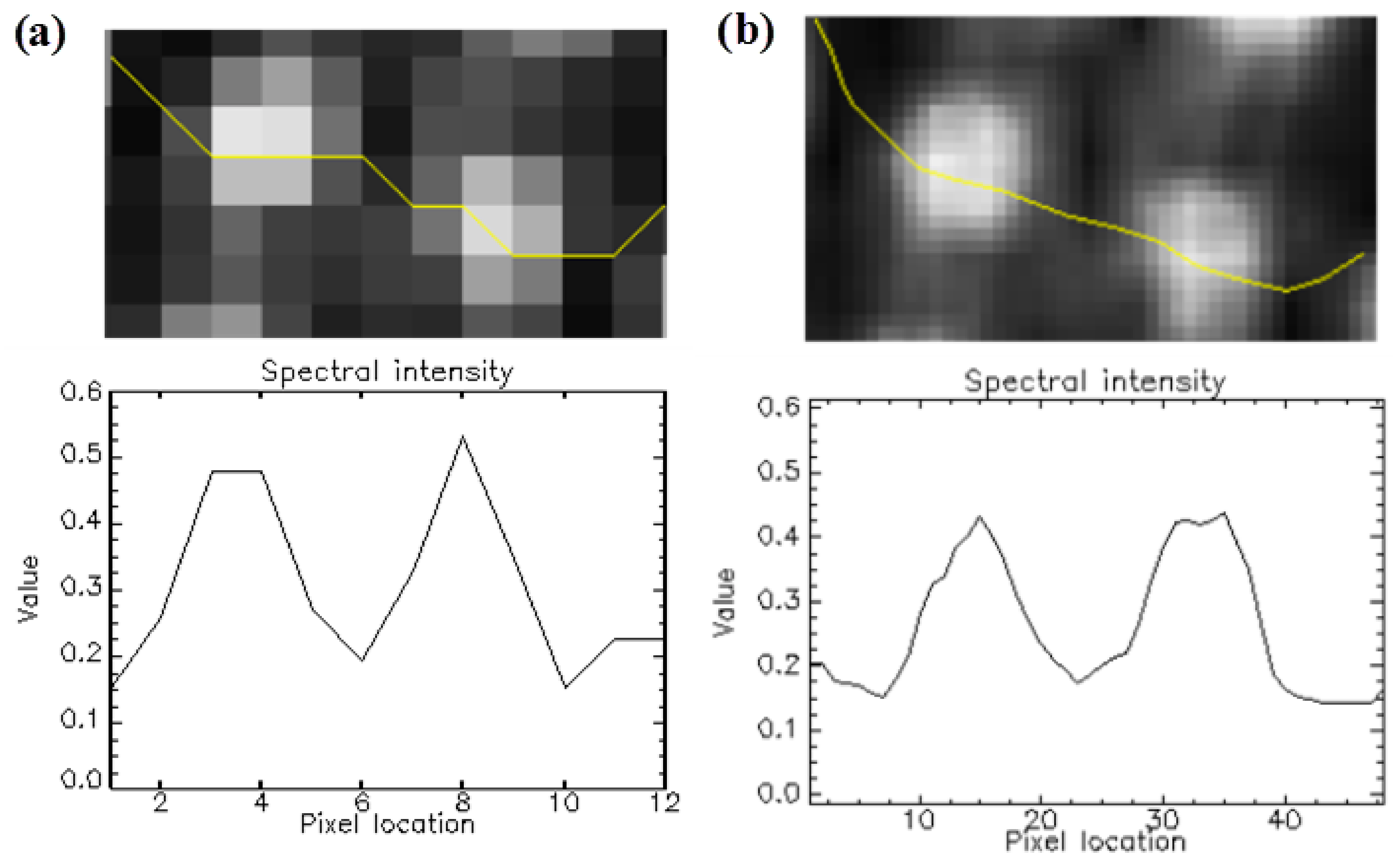
A tree in a remote sensing image can be described by a bell-shaped spectral profile. The position of the brightest peak is subject to the position of the sun and the satellite sensor. A relative transformation, such as normalized difference vegetation index (NDVI), corrects for the uneven sun illumination of the crown [30]. Then, a tree object is a bright region on a dark background in an image with a smoothly varying intensity profile and a maximum at the center of the tree (Figure 2). We call such an object a blob that can be expressed as a function of geographical coordinates and size of the tree .
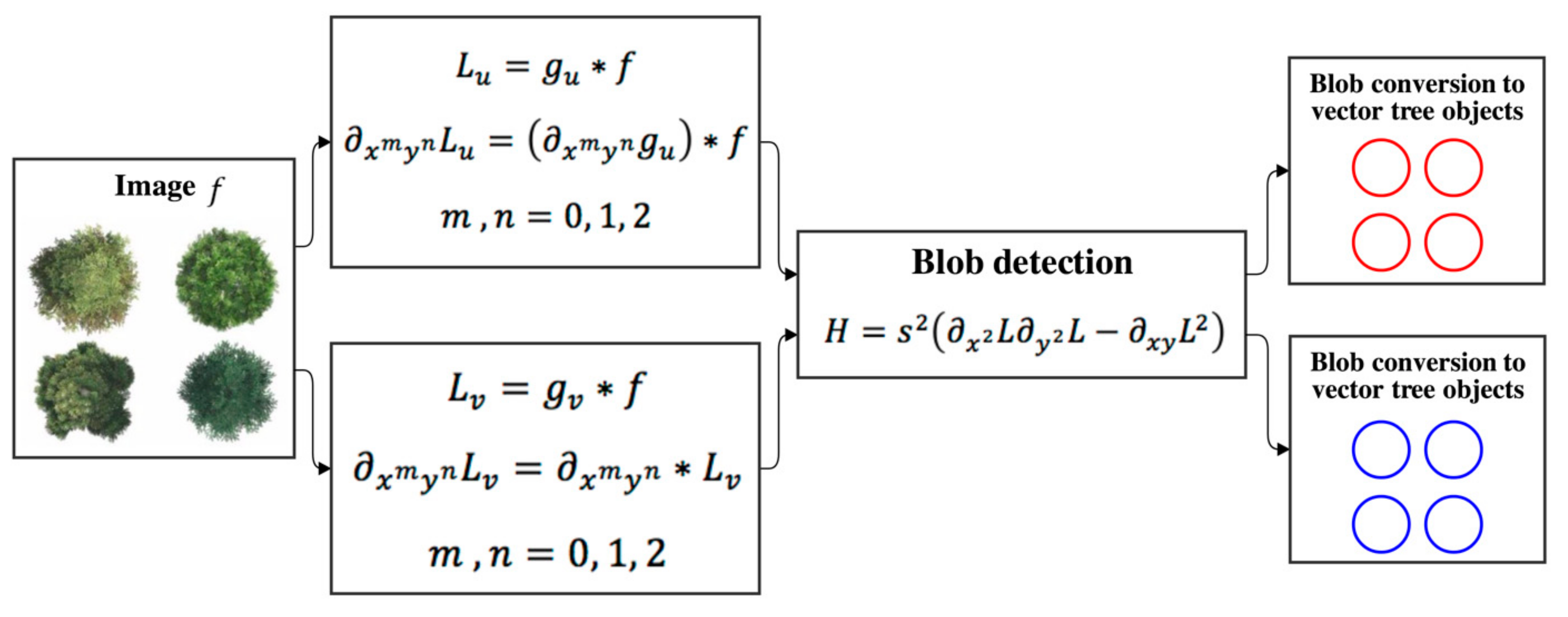
Figure 3 depicts how Gaussian scale-space theory is used for blob detection. Blobs are detected in scale-space using the local maxima of the scale-normalized determinant of the Hessian [31] as:
where . Due to the associativity of convolution, can be expressed as , i.e., the original image convolved by the kernel’s derivative , performing a single raster convolution operation in sampled Gaussian scale space. In contrast, the computation of a derivative in discrete Gaussian scale space requires an additional convolution operation, , where .
We denote a local maximum of H over scale by its position , and size . For a blob, . In the images, and have discrete values, and by interpolation the position of the local maximum is refined.
3. Modeling Tree Crown in the Scale Direction
3.1. Gaussian Blob Models
For the Gaussian blob, the intensity profile is modeled as a Gaussian bell-shaped surface function centered at and , and taking these values equal to 0, we obtain the following:
where describes the contrast between the blob and background, and the parameter is the background assumed to be constant, i.e., independent from and , and specifies the size of the Gaussian blob. A scale-space extension of Model (5) includes the scale parameter ,
substituting Model (6) into Model (4) and setting and , we obtain a response of a Gaussian blob in the scale direction as:
A major reason for considering the scale direction is that instead of the analysis of two-dimensional signal , we analyze a one-dimensional signal and the noise associated with the background and irregularities of the tree crown is limited to small values of . Model (7) is monotonically increasing for and decreasing for . Its maximum occurs at and equals:
A relatively simple model is the Gaussian blob model, where it is obtained from Model (7) as . To account for the sub-pixel shift between the Gaussian blob center and the discrete raster pixel location, we define as an adjustment to as:
The global maxima of model with respect to is attained at and , assuming .
3.2. Models for a Real Tree Crown
We observed in all our experiments that and are relatively crude approximations for real tree crowns especially for s > s0. To account for this, we modified the real tree model as by including a parameter :
This real tree model can again be shifted from the center by , yielding model as:
Upon implementation, the parameter δ is to be estimated, where δ ≠ 1 distinguishes f3(s) and f4(s) from f1(s) and f2(s), respectively. The global maxima of models f3(s) and f4(s) with respect to s are attained at s = s3 and s = s4, respectively. The physical interpretation of δ is that for increasing values of δ > 1 mainly the larger scales (s > s0) are affected. Therefore, introduction of δ leads to flexibility in the dependence modeling, where for larger values of s the dependence reduces.
3.3. Implementation
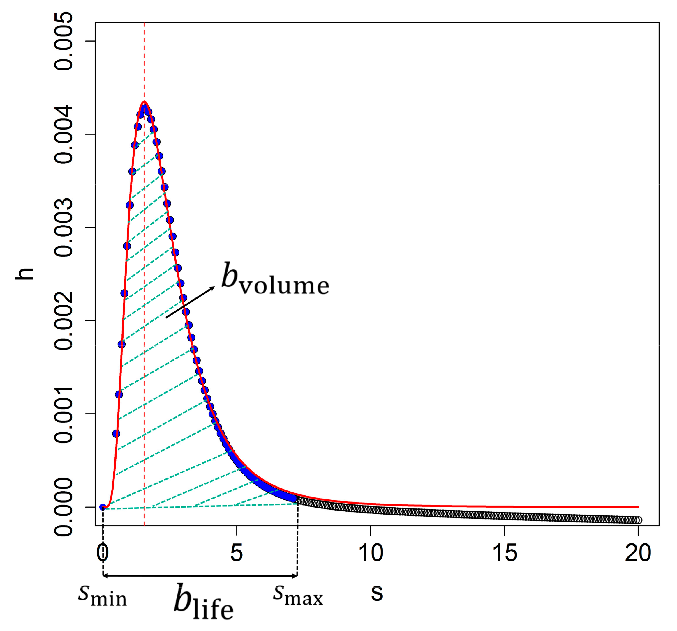
Upon implementation, we first identify the location of the local maximum with respect to space and scale on the discrete grid for and refine it to using polynomial second order interpolation. Next, we identify the range and corresponding to a single blob where is the lifetime. We do this by region growing into the direction s such that h(s) decreases if |s − s0| increases and h(s) exceeds a small positive threshold value (Figure 4). At s > s0, h(s) may include a contribution from the surrounding trees, for example, when several trees are found in a cluster. This contribution may affect fitting the models fk(s). Therefore, we limit the value to smax = 2s0. Fitting all models to the discrete observations {si,hi} in the range was done by numerically minimizing the sum of the squares cost function using L-BFGS-B [32] and the tree size rk from all four models is determined from sk = . The models (8)–(11) for h are proportional to a2, and therefore include dark objects (a < 0). We eliminate those by checking whether the scale-normalized Laplacian of the Gaussian scale space, i.e.,
is at a minimum or at a maximum at s0. This is achieved by checking the sign of the second derivative of the ∆L with respect to s. The volume of a blob, bvolume, is determined in the scale direction as:
being the area between smin and smax below h(s) (Figure 4). The blob volume is small for blobs with a low contrast with the background, whereas it is large for blobs with a high contrast. Relating blob volume to tree detection, we notice that a tree object has a larger scale-space volume, and hence the blob of a low volume can be discarded. In addition, the total relative error (εr) for all models used to discriminate larger blobs consists of several tree objects and it equals:
for k = 1, …, 4.
4. Uncertainty Assessment
Two uncertainty assessments were carried out to validate tree crown boundary detection, focusing on the presence and the spatial extent of individual trees. We follow [24] to accept the number of correctly detected tree objects, when the center of each falls within the spatial extent of the reference data for further analysis. Ref. [33] proposed over- and underestimation error metrics when assessing the area of a detected object with respect to the area of reference object , as:
and
respectively, where i indexes individual objects. Models (15) and (16) both result in values between 0 and 1, and there is a good match between detected and reference tree crown boundaries if these are close to zero. Furthermore, the total detection error is the following:
with . We consider three object accuracy indicators concerning the spatial extent of the tree objects, i.e., true positives (TP) where tree objects exist in the reference polygon layers, false positives (FP) that consider inappropriate detection where the trees are not present at the reference layer, and false negatives (FN) where there is a failure to detect objects in the reference layer [34]. The Euclidean distance (E) evaluates the distance between the centroid of a detected tree object and the centroid of a reference tree crown boundary as a positional accuracy indicator as:
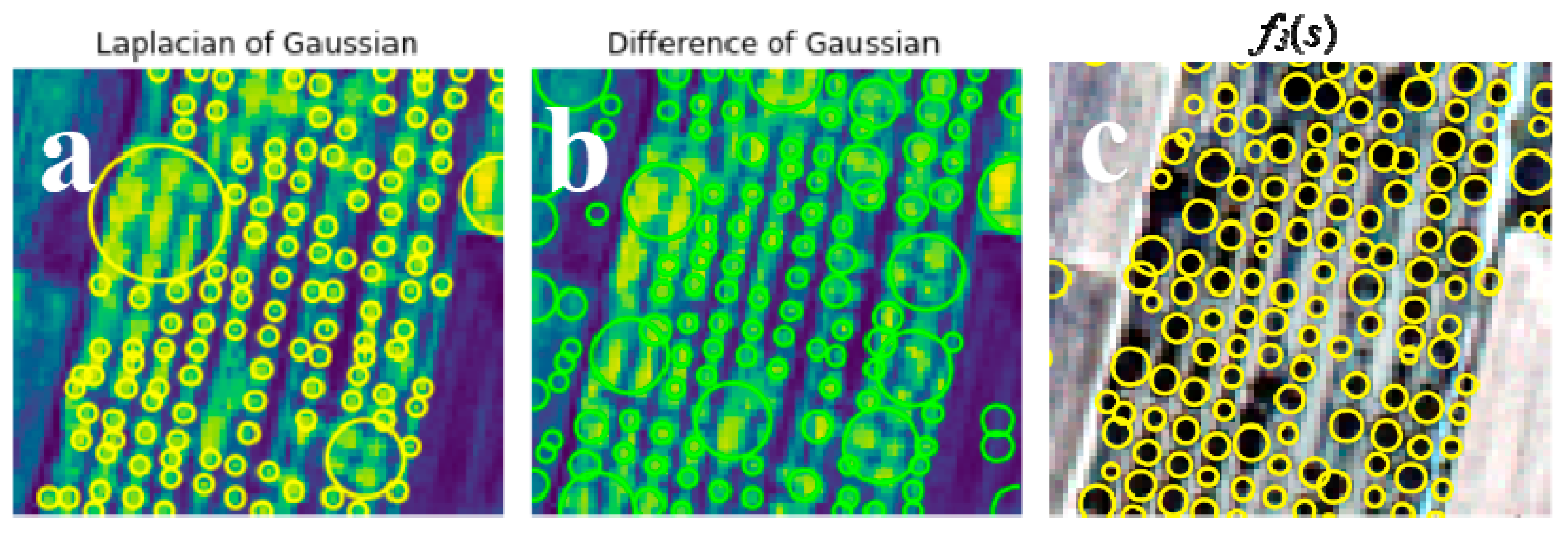
We compared the scale space method with two other techniques for individual tree crown blob detections, i.e., the Laplacian of Gaussian (LoG) technique [21], and the Difference of Gaussian (DoG) technique [35]. LoG obtains the Laplacian of Gaussian images with successively increasing standard deviation, stacking them in a cube where blobs are identified as local maxima. Detection of larger blobs, however, is slower because of the larger kernel sizes during convolution. Additionally, only bright blobs, i.e., objects with higher NDVI values, on a dark background are detected. DoG detects blobs by finding maxima in the matrix of the determinants of the Hessian of an image. Bright blobs, i.e., with higher NDVI values on a dark background as well as dark blobs, i.e., with lower NDVI values are detected. However, DoG suffers from the same disadvantage as LoG for detecting larger blobs.
5. Study Area, Data and Tools
5.1. The Walnut Orchard
The first study area is an orchard cultivated with walnut trees (Figure 5b) located in the Qazvin agricultural area in northwestern Iran with geographical coordinates 36°06ʹ N, 50°18ʹ E. The main reason for selecting this study site was the economic importance of the wood and nuts of the trees. The selected orchard contains trees of different crown shapes and sizes planted in rows. The study period was the middle of the growing season (July), when walnut tree crowns interlock with adjacent tree crowns. A four band (visible and near-infrared) multispectral image of WV-2 was taken on 7 July 2012, at a 2 m spatial resolution. An UltraCam digital image was collected on 17 July 2012 by a high resolution multichannel RGBI sensor, at a 0.5 m spatial resolution. The digital aerial image was delivered as an orthorectified image, corrected for lens distortion and camera tilt, and was co-registered to the panchromatic WV-2 image. The UltraCam image was used as a reference image for uncertainty assessment. For this validation, a polygon reference boundary layer was extracted manually from the UltraCam digital aerial photo using a visual interpretation.
5.2. Oil Palm Trees
The second study area is an orchard with oil palm trees (Figure 5c) planted in the Kutai Timur Regency, Kalimantan Timur province in Indonesia, located at geographical coordinates 00°58ʹ N, 118°03ʹ 0E. The oil palm trees are planted mainly with little differences in crown size and shape following a hexagonal pattern. The oil palm trees are commercially predominant in the food industry because of their fruit nutrition and oil production. A panchromatic image and a four band multispectral GeoEye image with visible and infrared bands were acquired on 25 May 2010, at a 0.5 m and a 2.0 m spatial resolution, respectively. The images were co-registered and projected in Universal Transfer Mercator (UTM) coordinates, with the standard spheroidal reference surface WGS84 and were geometrically corrected. The panchromatic GeoEye image was used as a reference image for validation. For this purpose, a polygon reference boundary layer was extracted manually representing the oil palm trees.
5.3. Vitellaria Trees
The third study area contains vitellaria trees (Figure 5a) located at 12°09ʹ N, 05°12ʹ 0W in Mali, commonly known as shea trees. This type of trees is found throughout Africa and their economic value is their oil rich seeds from which shea butter is extracted. In fact, the trees produce shea nuts for up to 200 years. A four band (visible and near-infrared) multispectral image of WV-2, and a panchromatic image were taken on 9 September 2015, at a 2 m and a 0.5 m spatial resolution, respectively. A polygon reference layer representing the vitellaria trees was manually extracted from the panchromatic WV-2 image.
5.4. Software
6. Results
6.1. Tree Detection in Discrete Gaussian Scale-Space
Figure 6 shows the four applied models on the walnut trees detecting tree objects. From Figure 6, we observe that f3(s) and f4(s) provide a better fit to the data than f1(s) and f1(s). Next, we observe that the difference between f3(s) (r = 0.653) and f4(s) (r = 0.654) is negligible in terms of the parameter s0 that is related to tree size as compared with reference data. Moreover, the local maximum s0 of f1(s) (r = 0.578) and f2(s) (r = 0.579) are different from those of f3(s) and f4(s). For accurate estimation of s0, one needs either a large number of points at scale levels si for local interpolation which is increasing computational time, or an accurate model, here f4(s).
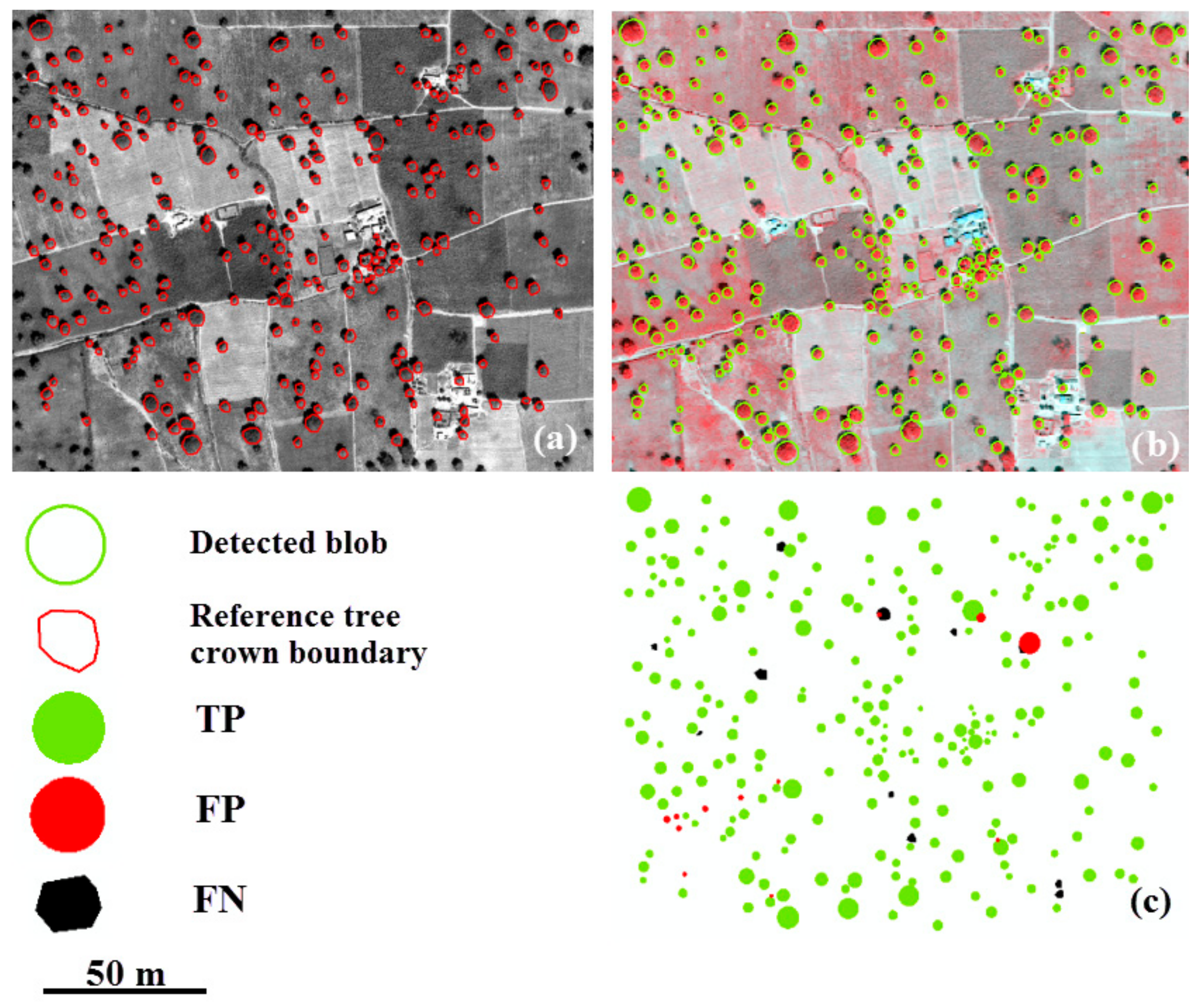
Table 1 gives the results in discrete Gaussian scale space using f3(s). It resulted in the detection of 391 individual trees out of 434 reference objects for the walnut orchard (90%), 252 individual trees out of 306 reference tree objects for oil palm trees (82%), and 238 trees out of 251 reference tree objects (94%) for vitellaria trees. FP error rates of 8.4%, 3.9%, and 5.0%, and FN error rates of 7.1%, 6.8% and 5.1% occur for walnut orchard, oil palm, and vitellaria trees, respectively. FN is lower for vitellaria trees because of the lower contrast between the trees and their background, whereas FP is lower for palm trees because of the low degree of interlocking adjacent tree crowns.
Figure 7, Figure 8 and Figure 9 illustrate the modeling of f3(s) for the different tree types, including a map of TP, FP, and FN. We observe that most trees have a different size parameter, ranging from 3.4 to 16.4 m for walnut, and from 1.5 to 19 m for vitellaria. Oil palm trees have similar range parameters, between 1.5 and 3 m. The high FP value for walnut (8.4%) is due to the regular tree pattern (Figure 7 and Figure 8). FNs for walnut and oil palm trees occur if adjacent tree crowns interlock, whereas, for vitellaria trees, they occur where the position of a detected blob centroid is outside the reference tree crown boundary.
Table 2 presents the positional inaccuracy of the different trees. For oil palm trees it is higher than for vitellaria trees, whereas for walnut trees the value of 0.91 m is slightly lower than that for vitellaria and oil palm trees. The reason is the different sun elevation angles during capturing of the VHR satellite images, resulting in small shadows, making identification of tree crown boundaries more difficult. Moreover, the aggregated and values for oil palm trees (0.42 and 0.33) are higher than those for walnut and vitellaria trees. The total detection error () is lower for both walnut (0.27) and vitellaria (0.33) trees than for oil palms, because of their larger tree size and because they are located in an area with a clear contrast between background and trees.
6.2. Comparison between the Sampled Gaussian Kernel and the Discrete Gaussian Kernel
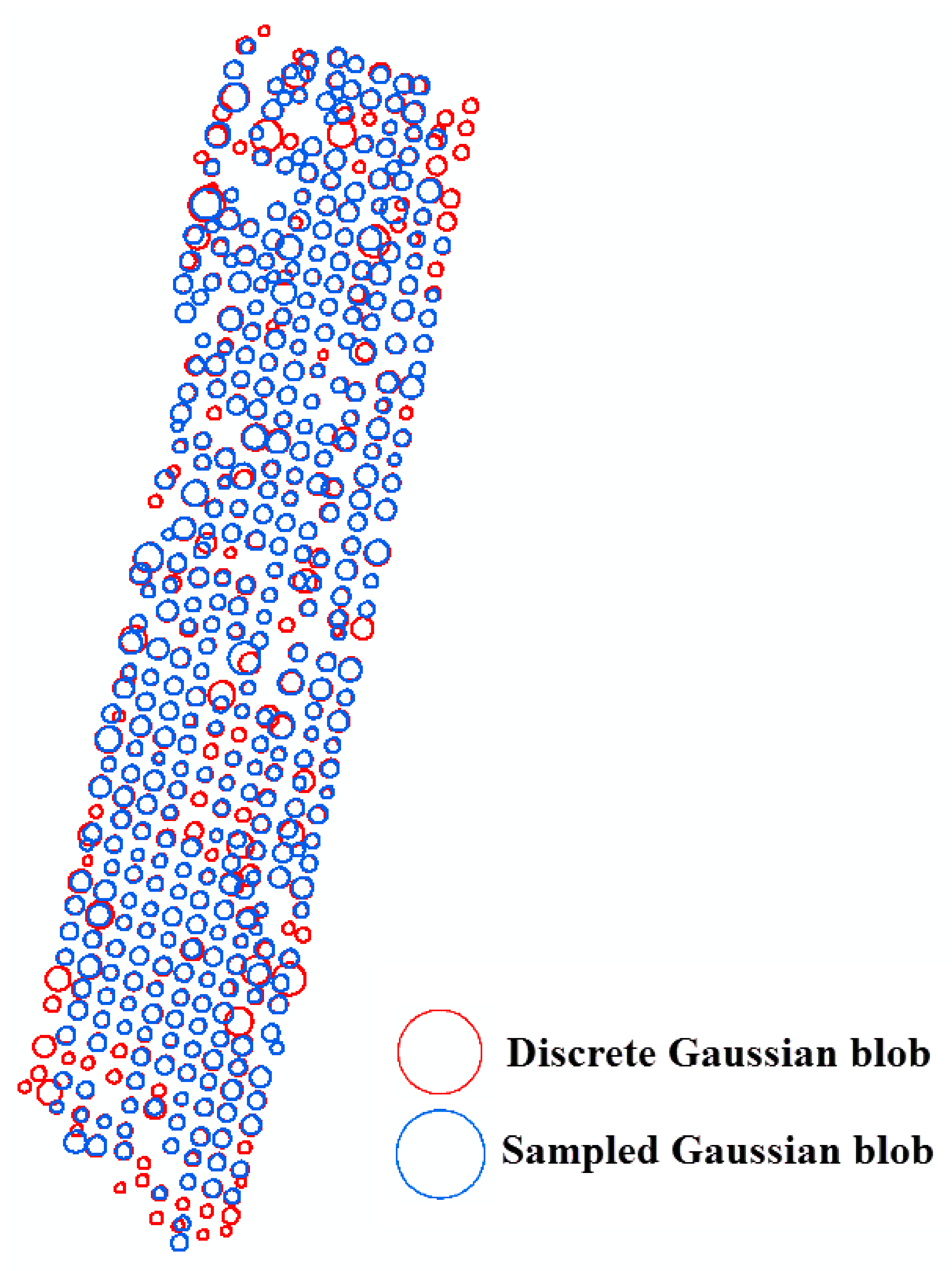
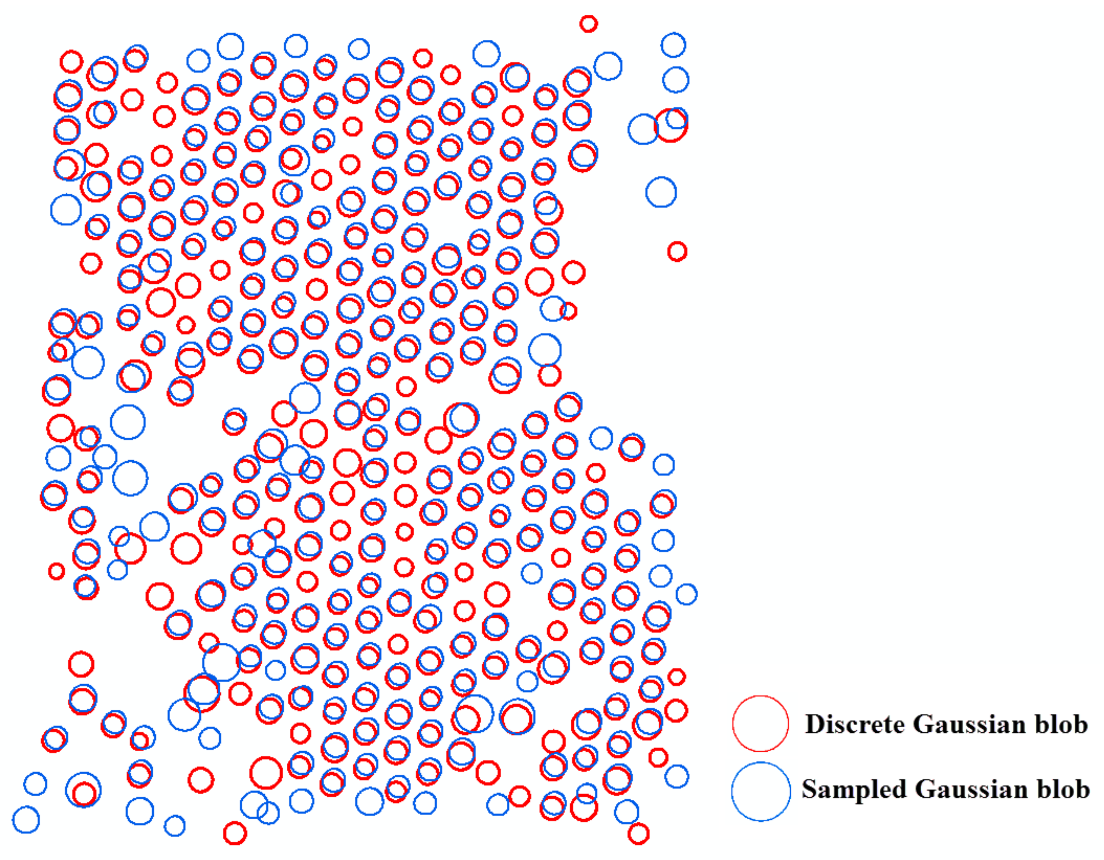
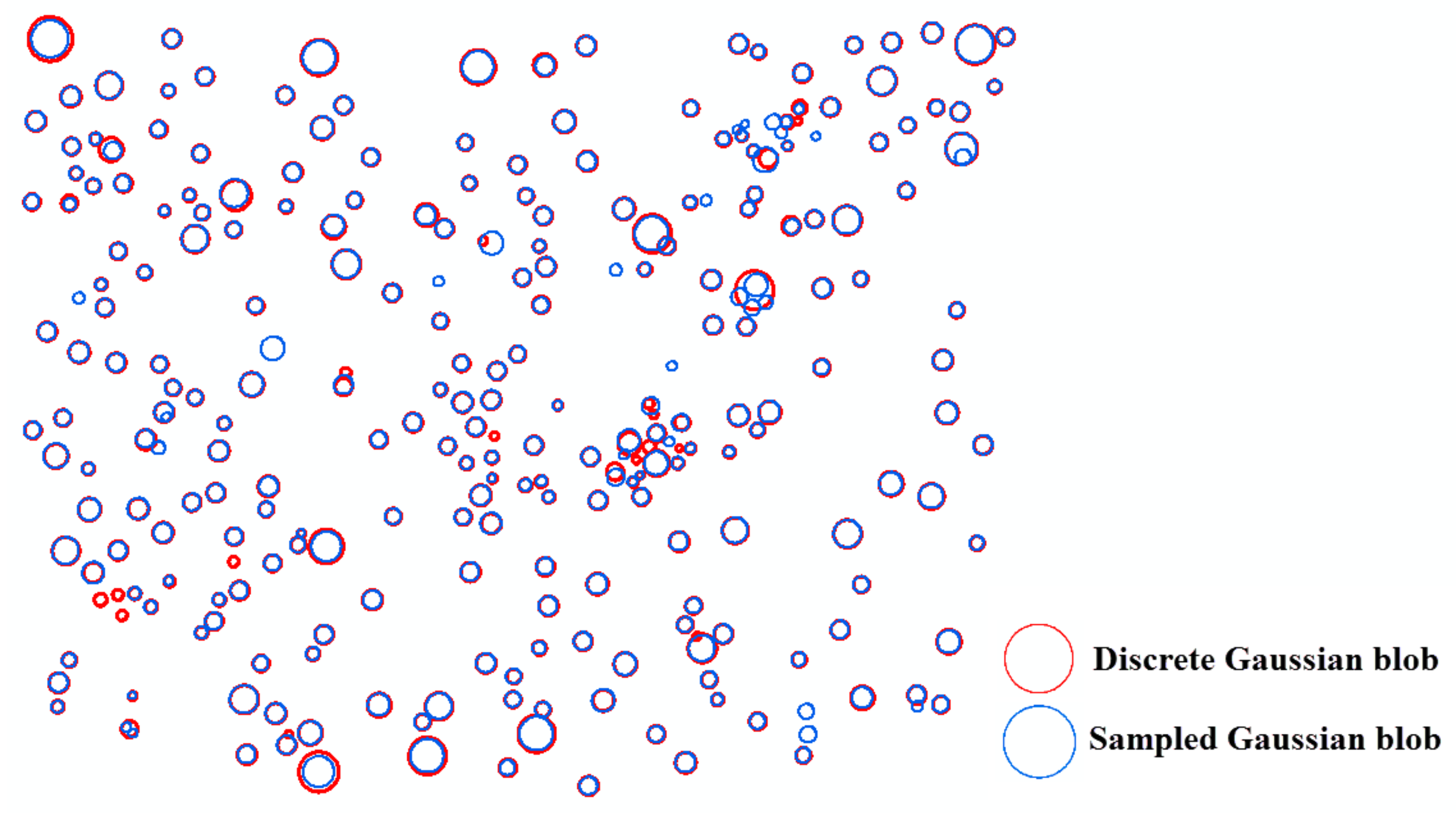
Figure 10, Figure 11 and Figure 12 compare the two-dimensional sampled Gaussian kernel gu and the two-dimensional discrete Gaussian kernel gv for walnut, oil palm, and vitellaria trees, respectively. Figure 10 shows that scale-space modeling with gv is capable of detecting 55 very small trees with a tree diameter lower than the pixel size as compared with the average size of walnut trees on the bottom and top rows of the orchard. The kernel gu performs better for the area where adjacent trees interlock. Figure 11 shows that, for oil palm trees, gv can detect 60 small trees more than gv in the hexagonal pattern, whereas gu performs better for detecting larger trees. For vitellaria trees, Figure 12 shows that gv detects 12 small trees, whereas gu is able to delineate trees with crown sizes that are larger than the pixel size. However, gv better approximates the local maxima at Model (4) when obtaining the derivatives at finer scales for small trees.
6.3. Comparison among Tree Crown Modeling, LoG, and DoG
Comparing the discrete Gaussian scale space using f3(s) for the walnut tree orchard (Figure 13), Table 3 shows that it detects 391 individual trees from 434 reference objects. LoG detects 356 individual trees (82%), whereas DoG detects 311 trees (72%). FP error rates equal to 11.2% and 14.9%, and FN error rates of 11.9% and 14% occur for LoG and DoG, respectively. For the discrede Gaussian scale space using f3(s), both FP and FN are lower, whereas its TP is higher. The reason is that it more precisely detects complex tree crowns where adjacent tree crowns interlock.
6.4. The Parameter δ for Different Tree Types
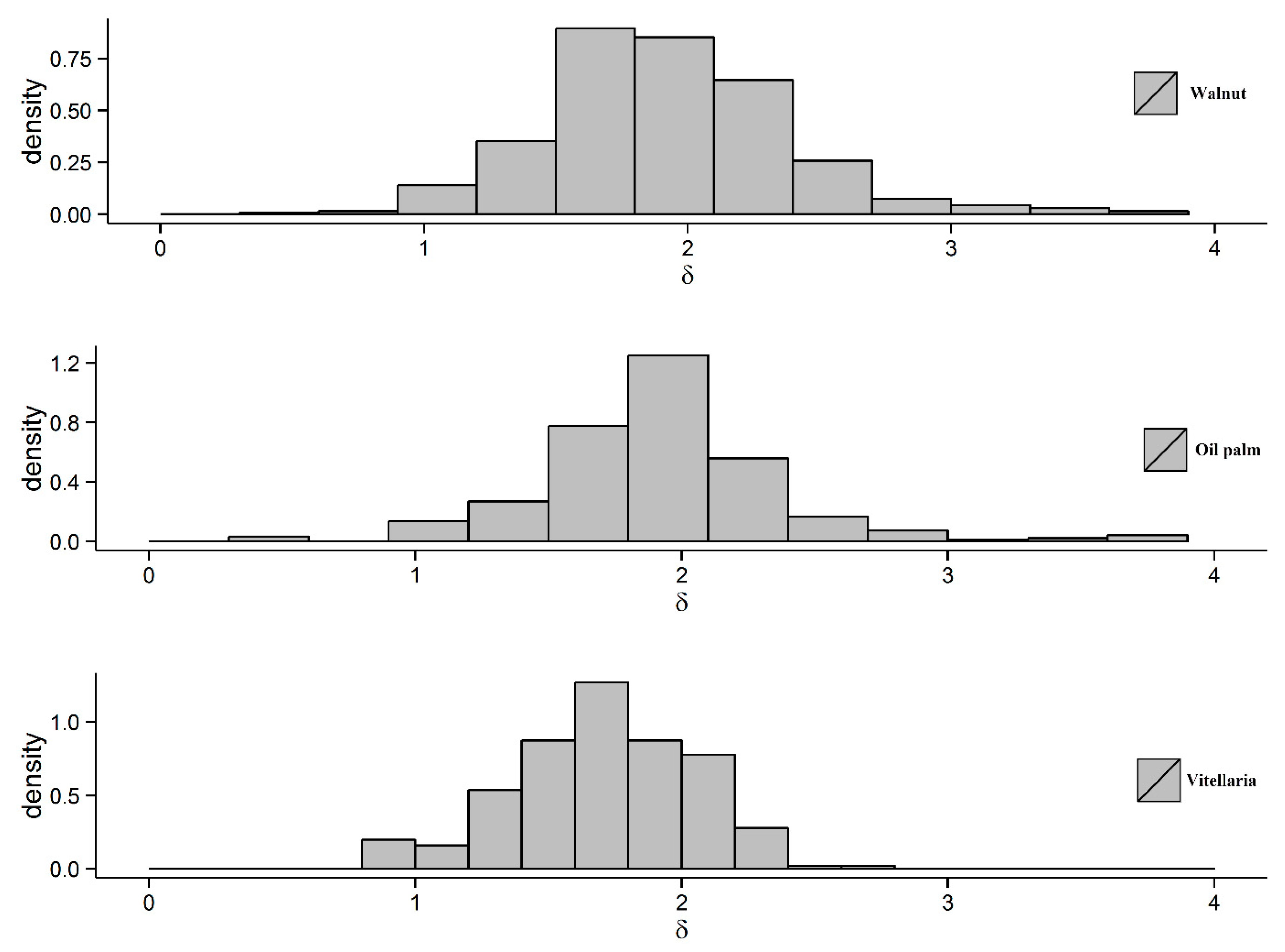
Figure 14 illustrates the density distributions of the parameter δ for different tree types, and for tree crown objects detected using f3(s) in discrete Gaussian scale space. For all the tree types, we observe a single mode for δ that is substantially larger than one. For vitellaria, the average δ is lower than for trees in the two types of orchards, whereas close values for δ are obtained for oil palm trees and for walnut trees. A likely explanation is that this is due to either tree species variation or irregularities in the spatial arrangement of the trees.
The following three hypothesises relate to the parameter δ:
Hypothesise 1(H1).
δ is related to the density of the trees, for example, the areas in an orchard, where trees are dense.
Hypothesise 2(H2).
δ is related to the contrast between a blob and the image background.
Hypothesise 3(H3).
δ is related to the tree size.
As concerns H1, we considered the relation between δ and the density expressed as the number of trees per unit area (DN) and the density defined as expressed as area of the trees per unit area DA. Table 4 shows DN and DA values for the three trees orchards. The vitellaria orchard has lower DN and DA values as compared with the walnut and palm orchards, and also the average value of δ for vitellaria is lower (Figure 14). Moreover, the δ values for the palm and walnut orchards are similar. We observed the highest DN value for the palm orchard, followed by the walnut and vitellaria orchards, whereas the DA value is higher for the walnut orchard that contains larger trees of varying sizes, in contrast to the palm orchard that has trees of similar sizes.
As concerns H2, we observed that both walnut and palm orchards have a lower contrast between trees and background image as compared with vitellaria trees. Moreover, vitellaria trees are planted with a higher irregularity as compared to walnuts and palms.
As concerns H3, we observed above that the parameter δ is insensitive of the left-hand side of h(s) (Figure 6).
7. Discussion
In this study, the intensity profile of a tree in the scale-space domain was characterized in an NDVI image by a bell-shaped surface as Gaussian blobs. The Gaussian blob models f1(s) and f2(s) inadequately described the trees, and their use caused overestimation and inaccurate tree size parameter estimation. The empirical models introduced in this paper, f3(s) and f4(s), provided a better description of the trees and more accurately estimated the tree size parameter s0. Indeed, models f3(s) and f4(s) adequately detected individual trees at the different scale levels (see Figure 6). All four models are asymmetric and in this sense their use extends local maximum interpolation as in [24]. Moreover, model f3(s) reduced the positional uncertainty of walnut trees from 103 cm in [24] to 91 cm in this study.
Models f3(s) and f4(s) provide a better fit to the data of Model (4) in the scale direction than models f1(s) and f2(s) because of the different δ values for individual trees. Differences between models f3(s) and f4(s) were negligible in this study, whereas the parameter Δr in f4(s) was affected by the resolution of the satellite image. For estimating trees under similar conditions as in this study, model f3(s) is to be preferred, as it is sparser and requires less input for estimating the tree crown parameters. In fact, model f4(s) more accurately estimates tree sizes as compared with model f3(s) with differences from 3 cm to 5 cm. This difference can be larger if coarse resolution pixels or smaller trees are considered.
Walnut and vitellaria trees both had a large variation in tree size. Figure 10 and Figure 12 show that in sampled Gaussian scale space we cannot detect trees with a slightly lower diameter than the pixel size of the image. The reason is that the local maxima of the blobs occur at finer scale levels than the image resolution. In contrast, in discrete Gaussian scale space, this problem is overcome, and we are able to also detect small trees at the finer scale level. In sampled Gaussian scale space, however, we are better able to delineate a large tree at coarser scale levels if adjacent trees interlock (Figure 10 and 11).
The scale-space representation Model (1) is the convolution between the discrete original image f and the Gaussian kernel (gu or gv). For both Gaussian kernels, the convolution is associative. By taking the derivative of the sampled Gaussian kernel we can either convolve it with the original image or reconstruct a sampled image f, and then obtain the derivative . As the derivative of the sampled Gaussian if . As a result, the derivatives in scale space cannot be correctly computed for fine scales, corresponding to the smallest trees. Therefore, for small values of s, we used gv in Model (1) to effectively obtain and detect small trees.
Comparing the results of the discrete scale space with the well-known LoG and DoG techniques, we found that both LoG and DoG resulted in higher FP and FN. The reason is that the discrete scale-space technique performs better for individual tree crown detection where a symmetric pattern is observed with patches of trees. Modeling of tree crown in the scale direction of the determinant of Hessian, therefore, resulted in a superior technique as compared with LoG and DoG.
We also compared the results of the presented scale-space methods with methods for tree detection in other studies. Brandberg and Walter [13] applied the multiple-scale algorithm to identify tree crown edge contours from local maxima on an aerial imagery at a 10 cm spatial resolution. For evaluation, they visually interpreted the mean area overlap between delineated and reference tree crown, resulting in an overall detection rate of 54%. In a forest area, Ref. [21] identified tree crown centers on two multispectral, pan-sharpened VHR satellite images, at a 60 cm spatial resolution. Using the estimated local maxima of the Laplacian in Gaussian scale-space on the classified RS imageries, they obtained detection rates of 93% and 86% for the first and the second images, respectively. Ref. [39] performed a plot-based method on the citrus orchard without tree crown interlock using aerial imagery, at a 50 cm spatial resolution. They combined image filtering with a weighted average filter and an unsupervised image classification followed by individualization of a tree using iterative local maximum filtering. They achieved an overall 90% detection rate, and a 40 cm positional error for individual trees. Ref. [40] used scale-space filtering on a papaya and a lemon orchard with isolated individual trees from images obtained by UAV. Applying the Laplacian of the Gaussian function resulted in a 95% detection rate for trees. FP (6%) and FN (5%) errors were due to multiple detections of a single tree, and even detection of a dead tree.
All these studies were done on individual trees and delineation was done for different forest types and various tree species. In addition, different sensors and RS images were used with varying spatial and spectral resolution, making it difficult to compare the methods. Our method is able to automatically detect individual tree crowns at a slightly higher detection rate. In addition, the refined model f3(s) in the scale direction provides an accurate estimation of tree parameters for three economically important tree species.
A final issue we want to address concerns the precise boundary of the tree crown, which is undefined and has an unstable estimation. We note that tree crowns have fragmented boundaries, and that stability of its estimate, and hence of the size of a tree and its position, depend upon the wind speed, canopy density, and noise in the background. To estimate tree size, our method reports the scale parameter, s0, assuming that a circular shape gives the crown radius of an individual tree. Trees, however, may have an ellipsoidal or a truncated cone crown shape, or even have an asymmetric crown in other environments, such as in natural forests, where tree species and management practices, such as pruning, differ from those considered in this study. Therefore, other types of tree shapes should be considered in future modeling of tree crowns in scale space. Furthermore, a tree crown is partially transparent and it has fractal properties with a boundary depending upon spatial resolution of the observations. Hence, the precise boundary of a tree crown cannot be defined in a strict sense. Moreover, this boundary is not static due to wind induced motion of branches and leaves and pruning of tree crowns could affect the shape.
A weakness of our method is that it is unclear whether it is able to address the presence of multiple maxima within a single tree. Multiple maxima can emerge due to several branches within a single tree. Trees may also be interlocking and form patches. This research can be extended by a more precise boundary estimation and extending the analysis towards identification of multiple maxima.
Our study aimed at trees in orchards and isolated trees in small holder agricultural crop fields. Variation in spectral response of a single tree crown may exist, related mainly to the variation in leave density. Such variation has two main components as follows: (1) A low frequency radial dependence and (2) high frequency irregularities of tree crowns. The low frequency component can be observed from VHR satellite images of trees with a crown diameter of a few pixels. Therefore, a future focus could be to develop a mathematical model that describes the low frequency components. There are multiple needs for such a model which include the following: (1) It is able to detect trees and distinguish them from uneven noisy background. (2) It may help to differentiate different tree species. (3) It may help to investigate overall tree stress, related, for example, to health or water shortage. (4) It allows accurate position determination of individual trees. (5) It is more accurate than simple boundary delineation, because the boundary can be affected by wind, and by the different looking angles of sensor. A full development for such models is outside the scope of the current paper and should be addressed in future research.
This research considered two orchards and an area with isolated tree crowns of different shapes, sizes, and species. The scale of management is important in precision agriculture, as modern management of nutrient and water supply focuses on treatment of individual trees. An improved detection of individual trees and delineation of their crowns, as shown in this study, could likely improve irrigation management, which depends upon the type and crown size of a tree, being, in most cases, a function of the tree cover fraction [41].
8. Conclusions
In this research, we improved Gaussian scale-space modeling for detecting and delineating individual trees from VHR images on three tree types at different continents. We did so by discretizing a Gaussian blob model in the scale direction, thus, proposing a discrete Gaussian scale-space model. In doing so, we were able to more accurately determine the tree size and discriminate between real tree objects and false detections. The main finding from this study was that our proposed model provides a better description of real tree crowns than the Gaussian blob model. Our method reduced the number of false negatives, and the discrete Gaussian scale-space model resulted in better detection of small trees. It further showed a substantial improvement as compared with existing techniques. In this way, our work improved upon the automatic detection and delineation of trees with varying tree crown sizes, which was more accurate than existing models.
Author Contributions
Conceptualization, M.M., V.T., and A.S.; methodology, M.M., V.T., and A.S.; formal analysis, M.M., V.T., and A.S.; writing—original draft preparation, M.M..; writing—review and editing, V.T. and A.S.; supervision, V.T. and A.S. All authors have read and agreed to the published version of the manuscript.
Funding
This research received no external funding.
Acknowledgments
The authors are grateful to the contributions of A. Sharifi, formerly at the faculty of Geo-Information Science and Earth Observation of the University of Twente, for his helpful comments and for providing the high resolution UltraCam image. The VHR WV-2 satellite image was provided by the STARS project, funded by the Bill & Melinda Gates Foundation, under grant #1094229.
Conflicts of Interest
The authors declare no conflict of interest.
References
- Ke, Y.; Quackenbush, L.J. A review of methods for automatic individual tree-crown detection and delineation from passive remote sensing. Int. J. Remote Sens. 2011, 32, 4725–4747. [Google Scholar] [CrossRef]
- Ardila, J.P.; Bijker, W.; Tolpekin, V.A.; Stein, A. Quantification of crown changes and change uncertainty of trees in an urban environment. ISPRS J. Photogramm. Remote Sens. 2012, 74, 41–55. [Google Scholar] [CrossRef]
- Erikson, M. Species classification of individually segmented tree crowns in high-resolution aerial images using radiometric and morphologic image measures. Remote Sens. Environ. 2004, 91, 469–477. [Google Scholar] [CrossRef]
- Pollock, R.; James, R. The Automatic Recognition of Individual Trees in Aerial Images of Forests Based on a Synthetic Tree Crown Image Model. Ph.D. Thesis, University of British Columbia, Vancouver, BC, Canada, 1996. [Google Scholar]
- Wolf, B.-M.; Heipke, C. Automatic extraction and delineation of single trees from remote sensing data. Mach. Vis. Appl. 2007, 18, 317–330. [Google Scholar] [CrossRef]
- Schardt, M.; Ziegler, M.; Wimmer, A.; Wack, R.; Data, L.S. Assessment of forest parameters by means of laser scanning. Int. Arch. Photogramm. Remote Sens. Spat. Inf. Sci. 2002, 34, 302–309. [Google Scholar]
- Persson, Å.; Holmgren, J.; Södermann, U. Detecting and measuring individual trees using an airborne laser scanner. Photogramm. Eng. Remote Sens. 2002, 68, 925–932. [Google Scholar]
- Pouliot, D.; King, D. Approaches for optimal automated individual tree crown detection in regenerating coniferous forests. Can. J. Remote Sens. 2005, 31, 255–267. [Google Scholar] [CrossRef]
- Chen, Q.; Baldocchi, D.; Gong, P.; Kelly, M. Isolating Individual Trees in a Savanna Woodland Using Small Footprint Lidar Data. Photogramm. Eng. Remote Sens. 2006, 72, 923–932. [Google Scholar] [CrossRef] [Green Version]
- Huang, H.; Li, X.; Chen, C. Individual Tree Crown Detection and Delineation from Very-High-Resolution UAV Images Based on Bias Field and Marker-Controlled Watershed Segmentation Algorithms. IEEE J. Sel. Top. Appl. Earth Obs. Remote Sens. 2018, 11, 2253–2262. [Google Scholar] [CrossRef]
- Hamraz, H.; Contreras, M.A.; Zhang, J. A robust approach for tree segmentation in deciduous forests using small-footprint airborne LiDAR data. Int. J. Appl. Earth Obs. Geoinf. 2016, 52, 532–541. [Google Scholar] [CrossRef] [Green Version]
- Gougeon, F.A. Automated individual tree crown delineation using a valley-following algorithm and rule-based system. In Proceedings of the International Forum: Automated Interpretation of High Spatial Resolution Digital Imagery for Forestry, Victoria, BC, Canada, 10–12 February 1998; Hill, D.A., Leckie, D.G., Eds.; Natural Resources Canada, Canadian Forest Service, Pacific Forestry Centre: Victoria, BC, Canada, 1999; pp. 11–23. [Google Scholar]
- Brandtberg, T.; Walter, F. Automated delineation of individual tree crowns in high spatial resolution aerial images by multiple-scale analysis. Mach. Vis. Appl. 1998, 11, 64–73. [Google Scholar] [CrossRef]
- Culvenor, D.S. TIDA: An algorithm for the delineation of tree crowns in high spatial resolution remotely sensed imagery. Comput. Geosci. 2002, 28, 33–44. [Google Scholar] [CrossRef]
- Pouliot, D.A.; King, D.J.; Bell, F.W.; Pitt, D.G. Automated tree crown detection and delineation in high-resolution digital camera imagery of coniferous forest regeneration. Remote Sens. Environ. 2002, 82, 322–334. [Google Scholar] [CrossRef]
- Popescu, S.C.; Wynne, R.H.; Nelson, R.F. Measuring individual tree crown diameter with lidar and assessing its influence on estimating forest volume and biomass. Can. J. Remote Sens. 2003, 29, 564–577. [Google Scholar] [CrossRef]
- Koch, B.; Heyder, U.; Weinacker, H. Detection of Individual Tree Crowns in Airborne Lidar Data. Photogramm. Eng. Remote Sens. 2006, 72, 357–363. [Google Scholar] [CrossRef] [Green Version]
- Culvenor, D.S. Development of a Tree Delineation Algorithm for Application to High Spatial Resolution Digital Imagery of Australian Native Forest. Internal Report. 2000. Available online: https://minerva-access.unimelb.edu.au/handle/11343/35186?show=full (accessed on 11 December 2020).
- Wulder, M.A.; Niemann, K.O.; Goodenough, D.G. Local maximum filtering for the extraction of tree locations and basal area from high spatial resolution imagery. Remote Sens. Environ. 2000, 73, 103–114. [Google Scholar] [CrossRef]
- Lindeberg, T. Feature Detection with Automatic Scale Selection. Int. J. Comput. Vis. 1998, 30, 79–116. [Google Scholar] [CrossRef]
- Skurikhin, A.N.; Garrity, S.R.; McDowell, N.G.; Cai, D.M. Automated tree crown detection and size estimation using multi-scale analysis of high-resolution satellite imagery. Remote Sens. Lett. 2013, 4, 465–474. [Google Scholar] [CrossRef]
- Wang, L. A Multi-scale Approach for Delineating Individual Tree Crowns with Very High Resolution Imagery. Photogramm. Eng. Remote Sens. 2010, 76, 371–378. [Google Scholar] [CrossRef]
- Witkin, A.P. Scale-space filtering. Int. Jt. Conf. Artif. Intell. 1983, 2, 1019–1022. [Google Scholar] [CrossRef] [Green Version]
- Mahour, M.; Tolpekin, V.; Stein, A. Tree detection in orchards from VHR satellite images using scale-space theory. In Proceedings of the SPIE 10004, Image and Signal Processing for Remote Sensing XXII, Edinburgh, UK, 26–29 September 2016; Bruzzone, L., Bovolo, F., Eds.; International Society for Optics and Photonics: Bellingham, WA, USA, 2016. [Google Scholar] [CrossRef]
- Wang, Y.; Zhu, X.; Wu, B. Automatic detection of individual oil palm trees from UAV images using HOG features and an SVM classifier. Int. J. Remote Sens. 2019, 40, 7356–7370. [Google Scholar] [CrossRef]
- Modica, G.; Messina, G.; De Luca, G.; Fiozzo, V.; Pratic, S. Monitoring the vegetation vigor in heterogeneous citrus and olive orchards. A multiscale object-based approach to extract trees’ crowns from UAV multispectral imagery. Comput. Electr. Agric. 2020, 175, 105500. [Google Scholar] [CrossRef]
- Lindeberg, T. Generalized Gaussian Scale-Space Axiomatics Comprising Linear Scale-Space, Affine Scale-Space and Spatio-Temporal Scale-Space. J. Math. Imaging Vis. 2010, 40, 36–81. [Google Scholar] [CrossRef]
- Lindeberg, T. Scale-Space. In Wiley Encyclopedia of Computer Science and Engineering; Wah, B.W., Ed.; John Wiley & Sons, Inc.: Hoboken, NJ, USA, 2008. [Google Scholar] [CrossRef] [Green Version]
- Lindeberg, T. Scale-Space for Discrete Signals. IEEE Trans. Pattern Anal. Mach. Intell. 1990, 12, 234–254. [Google Scholar] [CrossRef] [Green Version]
- Ardila, J.P.; Bijker, W.; Tolpekin, V.A.; Stein, A. Context-sensitive extraction of tree crown objects in urban areas using VHR satellite images. Int. J. Appl. Earth Obs. Geoinf. 2012, 15, 57–69. [Google Scholar] [CrossRef] [Green Version]
- Lindeberg, T. Scale Selection Properties of Generalized Scale-Space Interest Point Detectors. J. Math. Imaging Vis. 2012, 46, 177–210. [Google Scholar] [CrossRef] [Green Version]
- Byrd, R.H.; Lu, P.; Nocedal, J.; Zhu, C. A Limited Memory Algorithm for Bound Constrained Optimization. SIAM J. Sci. Comput. 1995, 16, 1190–1208. [Google Scholar] [CrossRef]
- Clinton, N.; Holt, A.; Scarborough, J.; Yan, L.; Gong, P. Accuracy Assessment Measures for Object-based Image Segmentation Goodness. Photogramm. Eng. Remote Sens. 2010, 76, 289–299. [Google Scholar] [CrossRef]
- Schuenemeyer, J.H.; Drew, L.J. Statistics for Earth and Environmental Scientists; John Wiley & Sons, Inc.: Hoboken, NJ, USA, 2010. [Google Scholar]
- Rafiee, G.; Dlay, S.S.; Woo, W.L. Region-of-interest extraction in low depth of field images using ensemble clustering and difference of Gaussian approaches. Pattern Recognit. 2013. [Google Scholar] [CrossRef]
- R Core Team. R: A Language and Environment for Statistical Computing; R Foundation for Statistical Computing: Vienna, Austria, 2017. [Google Scholar]
- Eddelbuettel, D.; François, R. Rcpp: Seamless R and C++ Integration. J. Stat. Softw. 2011, 40, 1–18. [Google Scholar] [CrossRef] [Green Version]
- Wickham, H. Ggplot2: Elegant Graphics for Data Analysis; Springer: New York, NY, USA, 2009. [Google Scholar]
- Recio, J.A.; Hermosilla, T.; Ruiz, L.A.; Palomar, J. Automated extraction of tree and plot-based parameters in citrus orchards from aerial images. Comput. Electron. Agric. 2013, 90, 24–34. [Google Scholar] [CrossRef]
- Jiang, H.; Chen, S.; Li, D.; Wang, C.; Yang, J. Papaya Tree Detection with UAV Images Using a GPU-Accelerated Scale-Space Filtering Method. Remote Sens. 2017, 9, 721. [Google Scholar] [CrossRef] [Green Version]
- Allen, R.; Pereira, L.; Raes, D.; Smith, M. Crop Evapotranspiration-Guidelines for Computing Crop Water Requirements; FAO Irrigation and Drainage Paper 56; FAO: Rome, Italy, 1998; p. D05109. [Google Scholar]
Figure 1.
Intensity profiles. (a) A coniferous tree with a single maximum; (b) A broad-leaved tree with several local maxima; (c) A noisy background; (d) Represents the fitted Gaussian functions after region growing between two interlocked trees, colored blue and red. The grey curve is obtained if the Gaussian function is fitted to all points, whereas the black curves are obtained if region growing is applied on the two separate tree objects.

Figure 2.
The spectral profile of tree crowns. (a) The NDVI image of WV-2 (2.0 m); (b) The NDVI image of WV-2 at 0.5 m spatial resolution.
Figure 2.
The spectral profile of tree crowns. (a) The NDVI image of WV-2 (2.0 m); (b) The NDVI image of WV-2 at 0.5 m spatial resolution.

Figure 3.
Schematic diagram of scale space for blob detection from either the two-dimensional sampled Gaussian kernel, indexed by , or the two-dimensional discrete Gaussian kernel, indexed by . The detected red and blue blob objects are from the sampled and discrete Gaussian kernels, respectively.
Figure 3.
Schematic diagram of scale space for blob detection from either the two-dimensional sampled Gaussian kernel, indexed by , or the two-dimensional discrete Gaussian kernel, indexed by . The detected red and blue blob objects are from the sampled and discrete Gaussian kernels, respectively.

Figure 4.
The blob volume bvolume and the blob lifetime blife. A blob volume is the area below the fitted model f3(s) at scale direction profiles h(s). The vertical dashed line indicates the location of the maximum t0 from model f3(s) (dashed line red color). Closed blue symbols show the range [smin, smax].

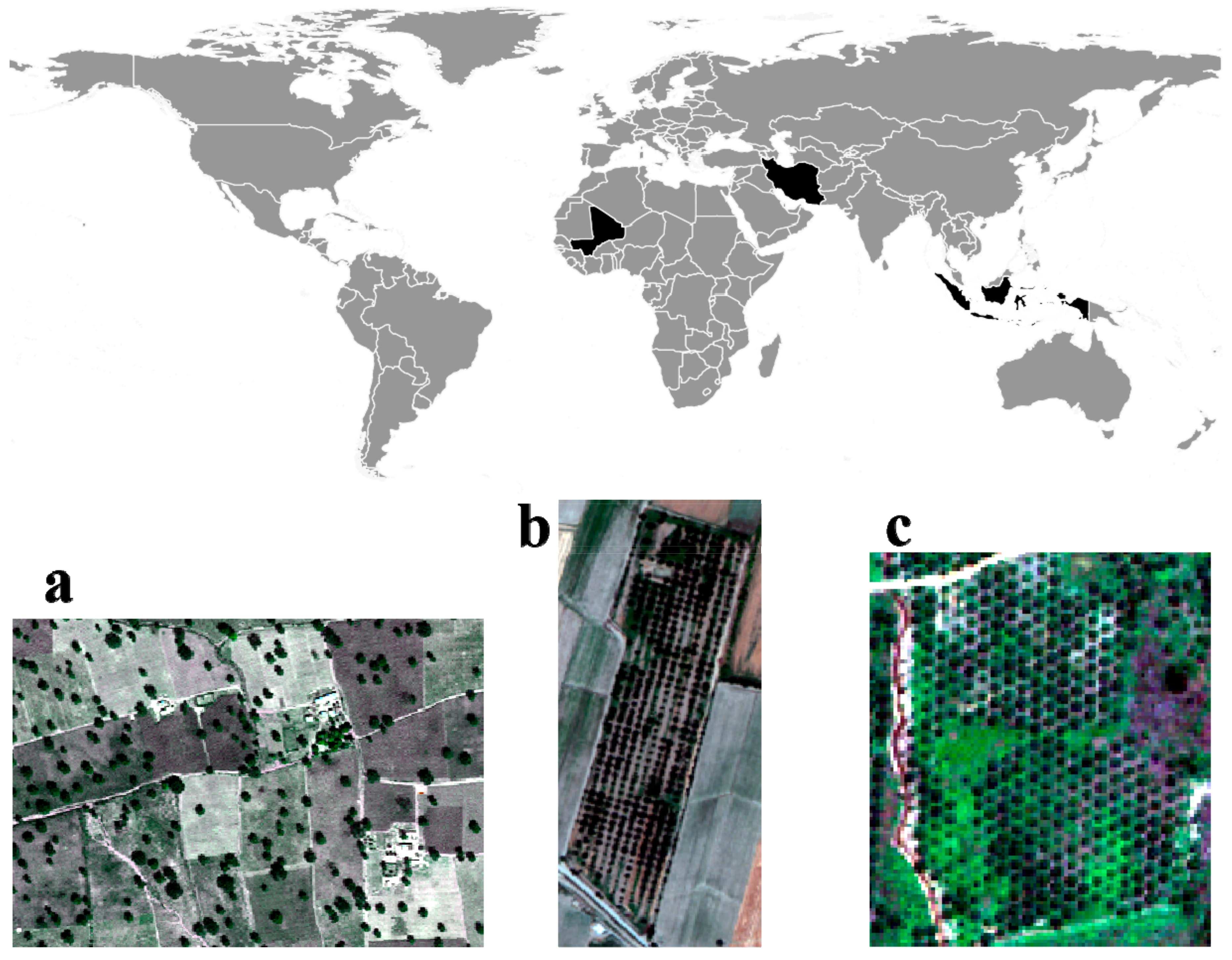
Figure 5.
Three orchards at different locations displayed as true color composite from satellite images. (a) Vitellaria trees in Mali; (b) Walnut trees in Iran; (c) Oil palm trees in Indonesia.
Figure 5.
Three orchards at different locations displayed as true color composite from satellite images. (a) Vitellaria trees in Mali; (b) Walnut trees in Iran; (c) Oil palm trees in Indonesia.

Figure 6.
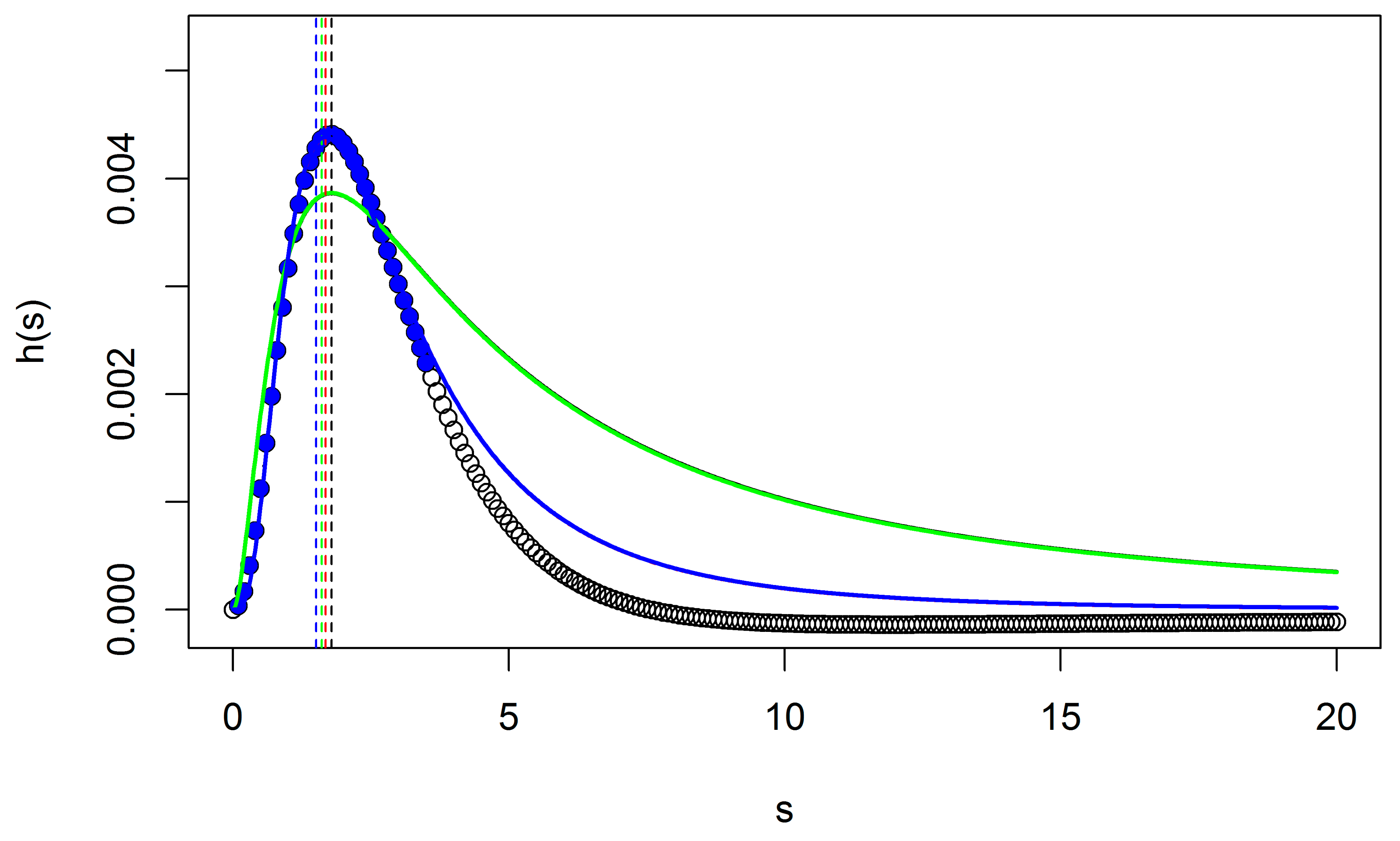
Scale direction profile h(s) for a real tree. The green line represents models f1(s), whereas the blue line represents f3(s). The red and black curve lines used for models f4(s) and f2(s) are invisible because their values are nearly identical to the blue and green curves, respectively. Green, black, blue, and red vertical dashed lines (left of the graph) indicate the location of the sk for the four models, whereas closed blue symbols show the obtained range [smin, smax].
Figure 6.
Scale direction profile h(s) for a real tree. The green line represents models f1(s), whereas the blue line represents f3(s). The red and black curve lines used for models f4(s) and f2(s) are invisible because their values are nearly identical to the blue and green curves, respectively. Green, black, blue, and red vertical dashed lines (left of the graph) indicate the location of the sk for the four models, whereas closed blue symbols show the obtained range [smin, smax].

Figure 7.
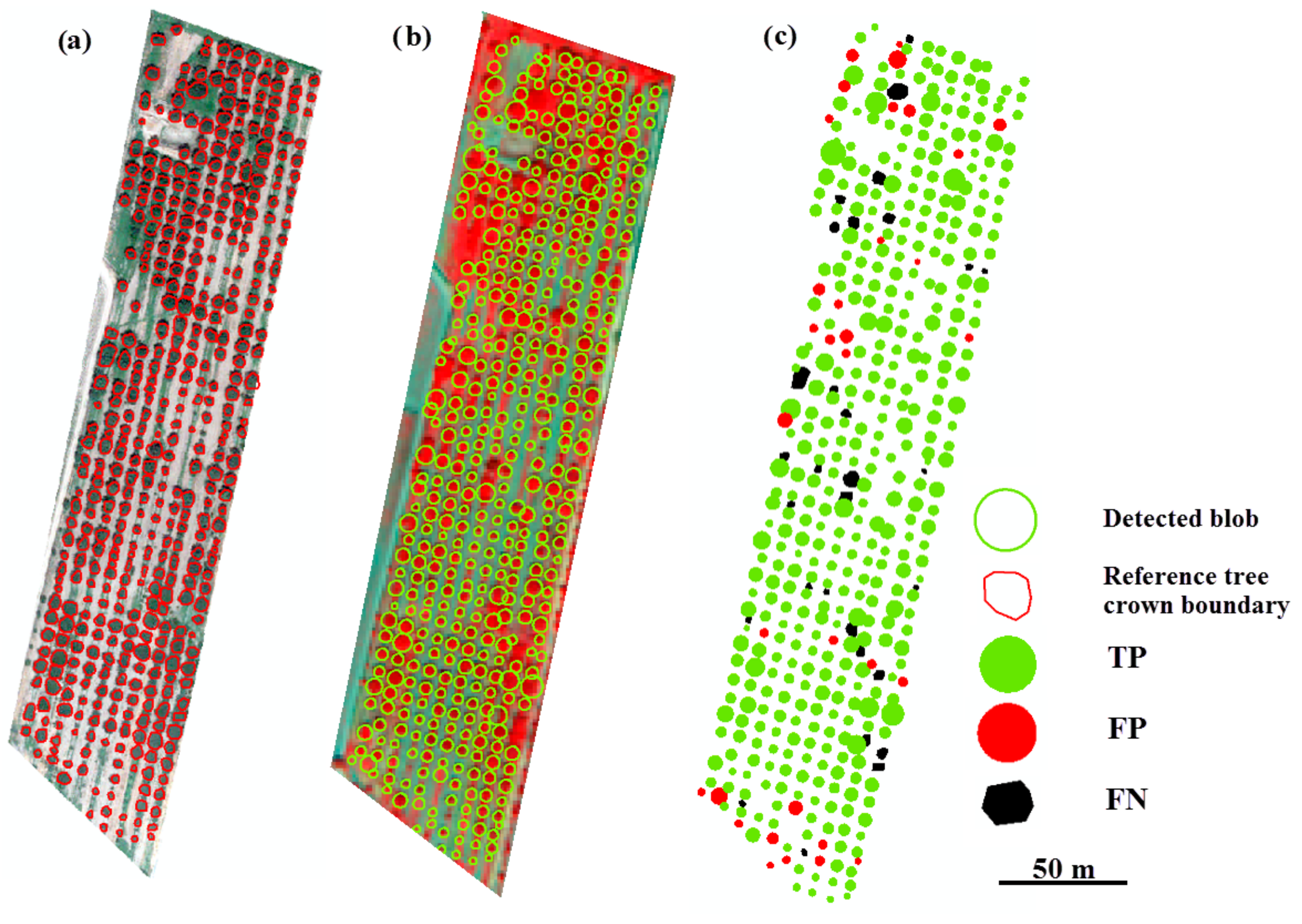
Results of tree detection in discrete Gaussian scale space with modified tree size measurement using model f3(s). (a) Reference data from an UltraCam image; (b) Walnut orchard with detected blobs; (c) The error map.
Figure 7.
Results of tree detection in discrete Gaussian scale space with modified tree size measurement using model f3(s). (a) Reference data from an UltraCam image; (b) Walnut orchard with detected blobs; (c) The error map.

Figure 8.
Results of tree detection in discrete Gaussian scale space with modified tree size measurements using f3(s). (a) Reference data from a panchromatic image; (b) The oil palm orchard with detected blobs; (c) The error map.
Figure 8.
Results of tree detection in discrete Gaussian scale space with modified tree size measurements using f3(s). (a) Reference data from a panchromatic image; (b) The oil palm orchard with detected blobs; (c) The error map.

Figure 9.
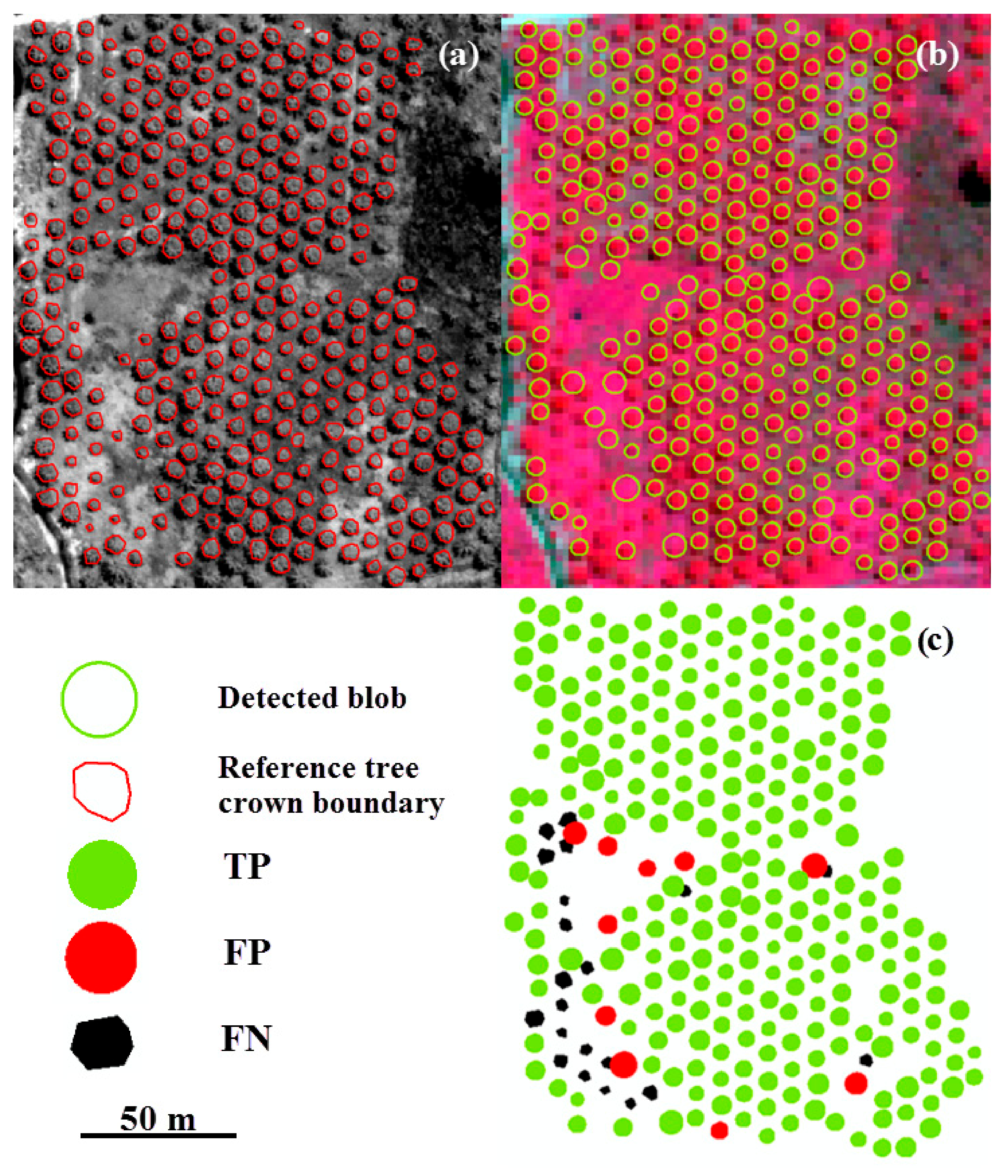
Results of tree detection in discrete Gaussian scale space with modified tree size measurements using f3(s). (a) Reference data from a panchromatic image; (b) Vitellaria trees with detected blobs; (c) The error map.
Figure 9.
Results of tree detection in discrete Gaussian scale space with modified tree size measurements using f3(s). (a) Reference data from a panchromatic image; (b) Vitellaria trees with detected blobs; (c) The error map.

Figure 10.
Differences between sampled and discrete Gaussian scale-space blob detection for the walnut orchard.
Figure 10.
Differences between sampled and discrete Gaussian scale-space blob detection for the walnut orchard.

Figure 11.
Differences between sampled and discrete Gaussian scale-space blob detection for the oil palm orchard.
Figure 11.
Differences between sampled and discrete Gaussian scale-space blob detection for the oil palm orchard.

Figure 12.
Differences between sampled and discrete Gaussian scale-space blob detection for vitellaria trees.
Figure 12.
Differences between sampled and discrete Gaussian scale-space blob detection for vitellaria trees.

Figure 13.
The Laplacian of Gaussian (LoG) technique (a), the Difference of Gaussian (DoG) technique (b), and (c) the discrete Gaussian scale space using f3(s) for the walnut tree orchard.
Figure 13.
The Laplacian of Gaussian (LoG) technique (a), the Difference of Gaussian (DoG) technique (b), and (c) the discrete Gaussian scale space using f3(s) for the walnut tree orchard.

Figure 14.
Distributions of parameter δ for different trees types obtained with model f3(s).


Table 1.
Detected tree objects based in discrete scale space, using model f3(s).
| Tree Types | Reference | TP | FP | FN |
|---|---|---|---|---|
| Walnut | 434 | 391 (90.09%) | 33 (8.43%) | 31 (7.14%) |
| Oil palm | 306 | 252 (82.35%) | 10 (3.96%) | 21 (6.86%) |
| Vitellaria | 251 | 238 (94.82%) | 12 (5.04%) | 13 (5.17%) |
Table 2.
Positional inaccuracy, overestimation, and underestimation metrics based upon the modified tree size measurement at s0 using model f3(s).
Table 2.
Positional inaccuracy, overestimation, and underestimation metrics based upon the modified tree size measurement at s0 using model f3(s).
| Tree Types | Positional [m] | [m] | [m] | [m] |
|---|---|---|---|---|
| Walnut | 0.91 | 0.32 | 0.13 | 0.27 |
| Oil palm | 1.50 | 0.42 | 0.33 | 0.57 |
| Vitellaria | 1.19 | 0.31 | 0.06 | 0.33 |
Table 3.
Detected tree objects based in f3(s) model, Laplacian of Gaussian (LoG), and Difference of Gaussian (DoG) for walnut tree.
Table 3.
Detected tree objects based in f3(s) model, Laplacian of Gaussian (LoG), and Difference of Gaussian (DoG) for walnut tree.
| Models | Reference | TP | FP | FN |
|---|---|---|---|---|
| f3(s) | 434 | 391 (90.09%) | 33 (8.43%) | 31 (7.14%) |
| LoG | 434 | 356 (82.02%) | 49 (11.29%) | 52 (11.98%) |
| DoG | 434 | 311 (71.65%) | 65 (14.97%) | 61 (14.05%) |
Table 4.
Densities expressed as the number of trees per unit area (DN) and as the area of trees per unit area (DA) for walnut, palm, and vitellaria trees.
Table 4.
Densities expressed as the number of trees per unit area (DN) and as the area of trees per unit area (DA) for walnut, palm, and vitellaria trees.
| Tree Type | DN | DA |
|---|---|---|
| Walnut | 0.00819 | 0.252 |
| Vitellaria | 0.00019 | 0.017 |
| Palm | 0.01126 | 0.220 |
Publisher’s Note: MDPI stays neutral with regard to jurisdictional claims in published maps and institutional affiliations. |
© 2020 by the authors. Licensee MDPI, Basel, Switzerland. This article is an open access article distributed under the terms and conditions of the Creative Commons Attribution (CC BY) license (http://creativecommons.org/licenses/by/4.0/).
Share and Cite
MDPI and ACS Style
Mahour, M.; Tolpekin, V.; Stein, A. Automatic Detection of Individual Trees from VHR Satellite Images Using Scale-Space Methods. Sensors 2020, 20, 7194. https://doi.org/10.3390/s20247194
AMA Style
Mahour M, Tolpekin V, Stein A. Automatic Detection of Individual Trees from VHR Satellite Images Using Scale-Space Methods. Sensors. 2020; 20(24):7194. https://doi.org/10.3390/s20247194
Chicago/Turabian StyleMahour, Milad, Valentyn Tolpekin, and Alfred Stein. 2020. "Automatic Detection of Individual Trees from VHR Satellite Images Using Scale-Space Methods" Sensors 20, no. 24: 7194. https://doi.org/10.3390/s20247194
Note that from the first issue of 2016, this journal uses article numbers instead of page numbers. See further details here.