Article

Soil Data Cube and Artificial Intelligence Techniques for Generating National-Scale Topsoil Thematic Maps: A Case Study in Lithuanian Croplands

by
Nikiforos Samarinas
1,*,
Nikolaos L. Tsakiridis
1,
Stylianos Kokkas
1,
Eleni Kalopesa
1 and
George C. Zalidis
1,2
1
Interbalkan Environment Center, 18 Loutron Str., 57200 Lagadas, Greece
2
Laboratory of Remote Sensing, Spectroscopy, and GIS, Department of Agriculture, Aristotle University of Thessaloniki, 54124 Thessaloniki, Greece
*
Author to whom correspondence should be addressed.
Remote Sens. 2023, 15(22), 5304; https://doi.org/10.3390/rs15225304
Submission received: 24 August 2023 / Revised: 31 October 2023 / Accepted: 7 November 2023 / Published: 9 November 2023
(This article belongs to the Special Issue Recent Advances in Remote Sensing of Soil Science)

Abstract

:
There is a growing realization among policymakers that in order to pave the way for the development of evidence-based conservation recommendations for policy, it is essential to improve the capacity for soil-health monitoring by adopting multidimensional and integrated approaches. However, the existing ready-to-use maps are characterized mainly by a coarse spatial resolution (>200 m) and information that is not up to date, making their use insufficient for the EU’s policy requirements, such as the common agricultural policy. This work, by utilizing the Soil Data Cube, which is a self-hosted custom tool, provides yearly estimations of soil thematic maps (e.g., exposed soil, soil organic carbon, clay content) covering all the agricultural area in Lithuania. The pipeline exploits various Earth observation data such as a time series of Sentinel-2 satellite imagery (2018–2022), the LUCAS (Land Use/Cover Area Frame Statistical Survey) topsoil database, the European Integrated Administration and Control System (IACS) and artificial intelligence (AI) architectures to improve the prediction accuracy as well as the spatial resolution (10 m), enabling discrimination at the parcel level. Five different prediction models were tested with the convolutional neural network (CNN) model to achieve the best accuracy for both targeted indicators (SOC and clay) related to the R 2 metric (0.51 for SOC and 0.57 for clay). The model predictions supported by the prediction uncertainties based on the PIR formula (average PIR 0.48 for SOC and 0.61 for clay) provide valuable information on the model’s interpretation and stability. The model application and the final predictions of the soil indicators were carried out based on national bare-soil-reflectance composite layers, generated by employing a pixel-based composite approach to the overlaid annual bare-soil maps and by using a combination of a series of vegetation indices such as NDVI, NBR2, and SCL. The findings of this work provide new insights for the generation of soil thematic maps on a large scale, leading to more efficient and sustainable soil management, supporting policymakers and the agri-food private sector.

Graphical Abstract

1. Introduction

Soil plays a vital role in supporting numerous essential ecological functions, encompassing sustaining crop production, nutrient cycling, carbon (C) storage, climate regulation, water purification, transfer of mass and energy between spheres, and acting as a habitat for diverse flora and fauna [1,2]. Healthy soils are the foundation of over 90% of the food we eat [3] and host 25% of all biodiversity on the planet [4]. Given the various physical (e.g., sealing, compaction, and erosion) and chemical (e.g., contamination, salinization, loss of organic matter) pressures exerted on soils, it is of paramount importance to preserve the soil ecosystem [5]. In the European Union (EU) alone, 70% of the soils are estimated to be in an unhealthy condition, with carbon loss, erosion, land take, and contamination being the major threats [6]. In July 2023, the EU proposed a new soil monitoring law [7]) to protect and restore soils and ensure that they are used sustainably; there is also a focus placed on defining what soil health is and the methodologies used to monitor it [8,9,10,11,12]. Additionally, soil’s capacity to sequester large amounts of C is taken into account, and techniques for monitoring soil carbon change are also widely examined [13].
Scientists, policymakers, and stakeholders alike acknowledge their critical responsibility in ensuring that soils maintain this capacity to sustain human life on the planet, and are developing tools to monitor the soil ecosystem [14]. These tools rely on large-scale Earth observation (EO) monitoring that leverages both the big geospatial data generated by space-borne missions and in situ monitoring [15,16,17], to provide accurate, timely, and objective information to support evidence-based conservation recommendations, which is crucial for creating a more sustainable future [18,19]. To process these large datasets various technological solutions have been proposed [20], with the datacube approach providing access to large spatio-temporal data in an analysis-ready form and offering the advantages of on-premises hosting and processing [21,22]. It has been successfully employed in areas ranging from helping farmers to manage their fields, over financial markets to forecasting food prices to the EU common agriculture policy [23], and in monitoring agricultural productivity [24].
When croplands are considered, bare-soil surface reflectance composites are usually constructed using a combination of thresholding and other heuristic methodologies from multispectral imagery [25,26,27]. The majority of studies usually take advantage of the spectral features of exposed soils over cropland areas, then apply various artificial intelligence (AI) algorithms to estimate the soil properties as derived from a compilation of soil samples. It is now even possible to provide high-spatial-resolution mapping using the European Copernicus Sentinels that provide images every 5 days at a 10 m resolution. To our knowledge, only a few studies have been conducted that have generated soil-related indicators at both a large scale and high spatial resolution [28,29]. However, these studies correspond to a coarse representation of the various soil properties, making their use impossible for good agricultural and environmental conditions (GAECs) [30] monitoring in the framework of cross-compliance, considering the small parcels in Europe. On the other hand, for permanently vegetated areas, the approaches followed consider mostly the usage of multiple environmental covariates (e.g., vegetation indices, climate data, geology, etc.) from which the soil properties are estimated [31,32,33], sometimes also incorporating radar data [34].
The recognized importance of sustainable soil carbon sequestration practices to contribute to climate change mitigation [35] has led to various applications of satellite EO data, demonstrating the benefits of EO-driven soil spatial products (reference). Two of the most widely monitored soil properties via EO are the soil organic carbon (SOC) and the clay content [36,37]. SOC is essential for a variety of soil processes and ecosystem services, plays a crucial part in the global carbon cycle, and is a topic of scientific interest in the context of climate change [38,39]. Estimating the geographical distribution of SOC content is essential for directing land management to improve soil health by reducing carbon emissions and sequestering C [40]. It may be significantly altered over the years due to crop practices. Soil clay content refers to the proportion of fine particles in the soil, and is one of the three soil particles that contribute to the soil’s texture (the other two being sand and silt particles). It is of crucial importance for soil health, influencing a soil’s fertility, water-holding capacity, nutrient availability, and overall soil structure, ultimately affecting plant growth and ecosystem functioning [41]. The clay content of soil typically does not change rapidly or frequently in natural conditions, being primarily determined by factors such as the parent material, weathering processes, and the geological history of the area. However, human activities, such as land management practices, can alter the clay content over longer periods of time; for example, excessive tilling or erosion can lead to a loss of topsoil, which may reduce the clay content.
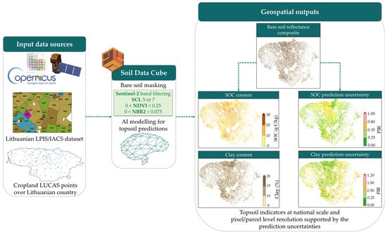
This paper aims to provide a novel pipeline for topsoil monitoring based on open-access EO data, artificial intelligence (AI), and advanced digital infrastructures, inspired by the demand for soil monitoring improvements with regards to its reliability (uncertainties) and spatial and temporal resolution. Differently from previous approaches that mainly focus on small- and medium-scale modeling, generating coarse-resolution products (>30 m), the main novelty of this work is its focus being mainly on the generation of national-scale soil thematic maps with high spatial resolution (10 m) based on an AI modeling approach. Specifically, this work will strive to:
  • Use multi-temporal Sentinel-2 imagery data for the identification of exposed soils over cropland areas, covering all of Lithuania at a 10 m spatial resolution.
  • Implement and evaluate AI algorithms for pixel-level predictions of the topsoil SOC and clay content in croplands at the national scale by using the Land Use and Coverage Area Frame Survey (LUCAS) dataset as ground truth soil data. A novel 3 × 3 padding scheme is used to augment the training dataset and provide more training data to the AI models. Moreover, two new CNN-based models predicting the two topsoil properties are introduced, whose network architecture is automatically optimized and that manage to outperform contemporary ML approaches.
  • Leverage the European Integrated Administration and Control System (IACS) database to transform the pixel-level predictions to more robust parcel-level estimations by proposing a novel thresholding methodology.
The proposed pipeline utilizes the Soil Data Cube (SDC), which is a self-hosted custom tool for the handling and processing of the large volume of satellite imagery data. At the same time, this work presents the main results and discusses the benefits, limitations, and perspectives of the proposed approach, while the overall methodology can be transferred and implemented in different bioclimatic zones and at various scales. Moreover, the parcel-level information could strongly support soil monitoring by national authorities and as part of different components of European policies, such as eco-schemes, in a more cost-efficient way.

2. Materials and Methods

2.1. Study Area

Lithuania is situated in the Baltic region of Europe and encompasses a total area of 65,300 km 2 . It is between the latitudes of 53° and 57°N and, for the most part, between the longitudes of 21° and 27°E (a portion of the Curonian Spit lies west of longitude 21°). It has around 99 km (61.5 miles) of sandy coastline, with just 38 km (24 miles) facing the open Baltic Sea, which is less than the other two Baltic nations. As for the agricultural sector, in 2016 it employed 255,570 people [42] while providing EUR 2.7 billion of 2022’s GDP [43], with the 2020 census reporting 29,145 km 2 as being used as agricultural land [44]. The main produce of Lithuania in 2020 was cereals (13,824 km 2 with 6.5 million tons) and wheat and spelt (8935 km 2 with 4.8 million tons), with fodder grasses and rape also being popular crops [45].

2.2. The Soil Data Cube Digital Infrastructure

2.2.1. Context and Background

The SDC is a custom digital infrastructure tool powered by the Open Data Cube (ODC) [46] aiming to generate analysis-ready data for soil monitoring at large scales by using EO technologies coupled with AI techniques. For further details of the SDC system architecture, the reader is referred to [47], while its web visualization engine is also available (https://portfolio.i-bec.org/eiffel/ accessed on 23 August 2023). Figure 1 presents the high-level view of the SDC flow, separated into three discrete steps:
  • Automate Sentinel-2 data acquisition: Sentinel-2 level 2A data over an area of interest and specific time period are downloaded from Copernicus and ingested into the Data Cube.
  • Pre-processing and data filtering: Bare-soil-reflectance composites are generated through masking the multi-temporal reflectance data using both the LPIS and IACS datasets and a bare-soil masking algorithm.
  • Modeling component: Generation of geospatial products (soil thematic maps) using the AI models trained on the LUCAS dataset.

2.2.2. Sentinel-2 Time Series Imagery Data Ingestion

The ingested data from the Copernicus Open Access Hub span 13 Sentinel-2 tiles to cover the entire country (Figure 2), while the maximum cloud coverage was chosen to be ≤30%. To provide yearly soil spatial explicit indicators for the period of interest (2020, 2021, and 2022) it is necessary to download the data from 2018 to 2022 (i.e., a five-year period). This need arises from the requirements of the bare-soil-reflectance composite product generation, which is produced based on the three year median value coming from the combination of the previous three annual bare-soil maps. Thus, for example, in order to generate the bare-soil-reflectance composite map for 2020, the imagery data from the years 2018, 2019, and 2020 are needed.

2.2.3. The European Integrated Administration and Control System (IACS)

To capitalize on open-access ground data, with a clear operationalization potential across the European territory, the European Integrated Administration and Control System (IACS) dataset is used, as it is the perfect source for discriminating agricultural fields. The Lithuanian IACS data utilized for parcel partitioning were made available by the Lithuanian National Paying Agency. The provided dataset includes farmers’ crop type declarations for the period of interest, along with a unique ID and the parcel’s geospatial information in vector format. It covers the entire Lithuanian territory, spanning more than 1,000,000 parcels per year. According to the 2022 IACS dataset, the four most common land-use classes are winter wheat (41%), winter rape (12%), spring wheat (8%), and spring barley (7%). The average parcel size is ≈3 ha, with the minimum and maximum sizes around 0.01 and 120 ha, respectively.

2.2.4. The LUCAS Topsoil Database

The Land Use and Coverage Area Frame Survey (LUCAS) of the European Soil Data Centre is a field survey program financed by the European Union’s Statistical Office that intends to collect and evaluate the major properties of topsoil in the 27 European Union member states [48]. It is considered as the biggest harmonized open-access dataset of topsoil properties at the global scale [48,49]. Four primary surveys have been conducted since the program’s inception: 2009, 2015, 2018, and 2022 (not yet publicly available). Technically, LUCAS 2009 has data from 23 member states (missing are Bulgaria, Romania, Malta, Cyprus, and Croatia, with the latter joining the union in 2013), the LUCAS 2012 topsoil survey only sampled Bulgaria and Romania with the same methodology as the one in 2009, while LUCAS 2015 and 2018 contain data from all of the then 28 member states (the United Kingdom is no longer part of the union as of the 1st of February 2020). The majority of samples were taken in 2009, and most sample points were revisited to assess changes in topsoil composition. A regular 2 km × 2 km grid covers the European territory, resulting in around 1,000,000 georeferenced sampling locations.
It should be noted that soil texture analysis (and particle size distribution) measurements were not conducted in LUCAS 2018. Moreover, in the LUCAS 2015 survey, the three fractions (sand, silt, and clay) were measured only at new LUCAS sampling points (i.e., points sampled for the first time in the LUCAS survey) because they are considered to be stable in the short to medium term. The particle size distribution was measured using laser diffraction following the ISO (International Organization for Standardization) procedure number 13320:2009 [50], whereas the organic carbon content was measured following the ISO 10694:1995 [51] protocol, i.e., determined after dry combustion with an elemental analyzer.

2.3. Data Processing and Modeling Using the SDC

2.3.1. Generation of the Bare-Soil Reflectance Composites

Recent studies [52,53] have indicated that bare surfaces detected by sophisticated analysis of multi-temporal remote sensing imagery data can be aggregated into soil reflectance composites to enhance the monitoring and mapping of cropland soils and their functions. Hence, frameworks based on EO data become fundamental to separate exposed soils from vegetated areas, as well as from non-photosynthetically active vegetation pixels. This process is an essential aspect of data preparation prior to modeling.
In this pipeline, the bare-soil reflectance composites are generated based on the three-year median value of annual bare-soil products. The decision to use multi-year composites was prompted by the missing pixel values that each annual product may introduce. In croplands, the bare soil occurs annually between March to October [54]. Due to severe weather conditions, and especially for North European countries such as our area of interest, the remainder of the year’s months are typically covered in snow, or crops are not cultivated for the most part. Therefore, the annual bare-soil products considered only the March–October period.
After compiling all the necessary satellite observations for each year, collected using the automated Sentinel-2 data acquisition of the SDC, the following step is to isolate the bare-soil areas. For a pixel to be identified as bare soil it must fulfill all of the three following criteria:
  • The Sentinel-2 scene classification layer (SCL): Twelve different classifications are provided by ESA and the Sen2Cor [55] package that generates the L2A products; in this work, the SCLs of not vegetated (SCL = 5) and unclassified (SCL = 7) were used, as both may correspond to bare-soil pixels and this filters out all unwanted classes (i.e., clouds, shadows, missing or defective data, snow, etc.).
  • Index thresholding: In order to further exclude vegetated and mixed pixels, the Normalized Difference Vegetation Index (NDVI) [56] and the Normalized Burn Ratio 2 (NBR2) [57] were used. Specifically, the NDVI must be strictly positive and less than 0.25 while NBR2 must be smaller than 0.075.
  • Heuristic band filtering (B1, B2, B3, B4): Due to the constant increase in the soil’s reflectance signature in the visible range, each RGB Sentinel-2 band must be larger than the one preceding it. Thus, B4 must be greater than B3 and B3 greater than B2. In addition, because the soil’s reflectance is low around 440 nm, B1 must have a reflectance value below 15%.
Pixels that do not match any of the above criteria are filtered out using a mask. Table 1 presents the overall filtering process for the final bare-soil reflectance composite generation.

2.3.2. Soil Modeling Using Artificial Intelligence Techniques

To estimate the soils’ physico-chemical properties from the soil reflectance composites, we tested five different machine learning models and used the ground truth LUCAS soil data. Each dataset (i.e., SOC and clay) was split randomly into 70% for training and 30% for testing. The hyperparameters of each learning algorithm were optimized using a 5-fold cross-validation grid search in the training set, as indicated below.
  • Random forest (RF) [58]: RF generates numerous decision trees that characterize with rules the relationship between the various features and the appropriate target variable. To optimize the hyperparameters of RF, a grid search was conducted as follows: the number of trees was selected from the {50, 100, 150, 200} set, while the maximum number of features to consider when looking for the best split was selected from the {“max”, “sqrt”, “log2”} set.
  • Support vector regressor (SVR) [59]: SVR is a supervised learning algorithm that utilizes support vector machines to perform regression tasks. It seeks to find the best-fitting hyperplane that maximizes the margin between the predicted targets and the actual targets, allowing for effective modeling of non-linear relationships and handling of outliers in the data. In addition to selecting the RBF kernel, the model was optimized through a grid search for its hyperparameters by examining the following values for ϵ : {0.01, 0.025, 0.05, 0.075, 0.10, 0.15, 0.20}, while the cost C was selected from { 2 2 , 2 1 , , 2 9 } .
  • Partial least square (PLS) [60]: PLS is one of the most commonly applied learning algorithms in spectral datasets where multicollinearity, i.e., correlations between explanatory variables, is probable. PLS has only one hyperparameter, namely, the number of latent variables; to optimize it we searched within {1, 10}.
  • Cubist [61]: Cubist is a machine learning technique that combines decision trees and rule-based models to create accurate predictive models. It employs a rule-based framework to generate interpretable and transparent models while handling complex datasets and capturing non-linear relationships between variables. It further adds corrections to the predictions based on the samples’ nearest neighbors. Its hyperparameters were optimized as follows: the number of committees was selected from {1, 5, 10, 20}, while the number of neighbors from {1, 5, 9}.
  • Convolutional neural network (CNN) [62]: A custom 1-D CNN was developed; to identify the optimal network architecture, the HyperBand optimization algorithm was employed [63], to avoid the exceedingly demanding computational cost of the full-grid-search solution. The following network parameters were searched for: (i) the usage of input standardization from {none, min–max, standard score}; (ii) the number of convolutional layers { 1 , 2 , 3 , 4 } ; (iii) the kernel size { 3 , 4 , , 7 } ; (iv) convolutional units (optimized separately for each layer) { 16 , 18 , , 64 } and use of dropout or max pooling of size 2; (v) the number of fully connected layers { 1 , 2 , , 5 } ; (vi) the number of neurons (optimized separately for each layer) { 16 , 24 , , 256 } and the activation function used, from {tanh, linear, Leaky ReLU}, where in the latter the slope coefficient is also optimized from [ 0.01 , 0.3 ] ; (vii) the batch size { 16 , 32 , 64 } ; and (viii) the learning rate, in [ 0.0001 , 0.01 ] using a log space. The Adam optimizer was used to minimize the loss function (mean squared error), and a maximum number of 100 epochs was used.
Furthermore, all the aforementioned models were trained with the SNV (standard normal variate) [64] and ABS (absorbance) [65] spectral pre-processing treatments for the input Sentinel-2 spectra bands, including the combination thereof (ABS+SNV).

2.3.3. From Pixel- to Parcel-Level Decisions

The aforementioned pipeline generates pixel-based products at a resolution of 10 × 10 m, providing detailed information on the quantification of SOC and clay in Lithuania’s croplands for the composite maps (2020, 2021, and 2022). Zonal statistics are then applied to these predicted topsoil maps, utilizing metrics such as median and valid pixel count, projected onto the IACS dataset to derive final values for each parcel. The two main metrics employed are the median value and the number of valid pixels, with filters applied to exclude parcels with no topsoil property pixels and to retain polygons meeting the area and coverage conditions. Specifically, polygons with at least one valid pixel and a shape area ≤ 1 ha are retained, while for larger areas the coverage is first calculated as follows:
coverage = pixel count · 100 shape area ( m 2 ) · 100
Then, two distinct conditions are imposed in order to retain the relevant components. The SOC map will retain portions that are >1 ha and have a coverage of at least 70%, while the clay map will retain parcels that are greater than 1 ha and have coverage ≥ 30%. The choice of these percentages was made based on our expertise and under the reality that SOC presents greater variability within the parcel compared to clay, and that is why the SOC percentage is more strict. We considered it misleading to give final values to parcels for which the area is >1 ha but the total number of pixels within the polygon is poor (e.g., 5 pixels). For explanation purposes, we created the example of Figure 3, where zonal-statistics-filtered parcels with a pseudocode explanation are provided.

2.3.4. Model Performance Metrics

The models were validated on the independent test set using the following metrics:
  • The coefficient of determination R 2 , which quantifies the degree of any linear correlation between the observations and the model-predicted output; it usually ranges from 0 to 1 (higher is better) and is calculated as follows:
    R 2 ( y , y ^ ) = 1 i = 1 N ( y i y ^ i ) 2 i = 1 N ( y i y ¯ ) 2
    with y ^ i being the prediction for the ith pattern, y i its ground truth value, and y ¯ the mean ground truth value across all N patterns.
  • The root mean squared error (RMSE), which is calculated via
    RMSE ( y , y ^ ) = i = 1 N ( y i y ^ i ) N
  • The ratio of performance to interquartile range (RPIQ), which takes both the prediction error and the variation in the observed values into account, without making assumptions about the distribution of the observed values. It is defined as the interquartile range of the observed values divided by the RMSE of the predictions [66]:
    RPIQ ( y , y ^ ) = Q 3 Q 1 RMSE ( y , y ^ )
    where Q 1 is the lower quartile or the 25th percentile of the data, whereas Q 3 is the upper quartile, which corresponds to the 75th percentile.

2.3.5. Model Uncertainty

In order to calculate and to visualize the model’s uncertainty as a map, we used the prediction interval ratio (PIR) [32]. In essence, multiple (in this case, 100) models, using bootstrap resampling, are developed, i.e., each trained on a randomly sampled subset of the available training data, and the distribution of the models’ predictions on each pixel enables the estimation of the underlying uncertainty. PIR is calculated as follows:
PIR = p 95 p 5 p 50
where p 95 and p 5 are the 95% and 5% percentiles, respectively, and p 50 is the 50th percentile or the median of the predictions. Following the PIR formula, the model’s uncertainty under 0.50 identifies a robust model with reliable predictions. Through this information, the end user can determine the critical points that need further investigation (e.g., physical sampling), and the researchers can further investigate the data that caused high uncertainty, hopefully leading to a more precise and accurate model. In the framework of this work, the PIR of the best model will be provided.

3. Results

3.1. Earth Observation Data Processing via the SDC

A total of 2262 Sentinel-2 images were ingested into the SDC, corresponding to approximately 5 terabytes, which cover Lithuania from 2018 to 2022 (5-year period) from March to October. Figure 4 demonstrates the number of images that were automatically downloaded for each year and per tile. The main reason behind the variance in the file counts per year is the cloud coverage filter of the SDC that assures that overcast scenes (i.e., with cloud coverage >30%) will not be further processed.
With respect to the ground truth data, all available LUCAS topsoil data from Lithuania were initially considered. LUCAS 2009 has 356 points, LUCAS 2015 has 353 points, and LUCAS 2018 has 386 points. All points from the 2018 survey are shown in Figure 5, which represents 51% of the whole Lithuanian dataset as croplands (196 points), 25% as grasslands (98 points), 23% as woodlands (89 points), and 1% as barelands (3 points).
Due to the fact that SOC content changes frequently over time, only the LUCAS 2018 cropland data were considered for this property. On the other hand, soil texture changes at a slow pace; therefore, for the clay content all available LUCAS topsoil data of the croplands were employed. Therefore, two different datasets are considered with a varying number of labeled data for the two soil properties. Table 2 provides summary statistics about both datasets.
To enlarge the training set and for robust modeling, a 3 × 3 pad of neighboring pixels was considered around the original LUCAS points. Each dataset was augmented by nine times based on the assumption that the neighboring pixels share the same indicator value [67]. This step leads to 1746 sample points for SOC and 1341 for clay. Using the SDC, the Sentinel-2 reflectance was extracted for each point from 2018 to 2022 in the months March–October. The 1746 samples of SOC yielded 203,565 different observations throughout the required time period, whereas the 1341 clay content samples yielded 182,299 data. These observations are the total data collected from Sentinel-2, irrespective of whether they represent bare-soil pixels or not.

3.2. Exposed Soils over Lithuania

A pre-processing workflow based on the threshold analysis, explained in Table 1, was applied to the acquired imagery data to first generate the annual bare-soil maps. Each annual map represented the spatial distribution of bare-soil areas for a specific year within the study period. More than 1 billion pixels per product were gathered to cover the entire cropland area of Lithuania. Once the annual maps were produced, the bare-soil reflectance composite map was generated by employing a pixel-based composite approach to the overlaid annual maps. Figure 6 illustrates, as an example, the final bare-soil reflectance composite map at the national scale for 2020, generated considering the median value of the three years 2018, 2019, and 2020.
Based on the composite map we can observe that the central hinterland presents a higher density of bare-soil pixels as Lithuania’s main agricultural area is located there. On the other hand, on the two bordering sides (west–east) of the country, a sparse density of bare soil was found, as the areas mainly consist of forest, grasslands, and wetland areas.
Furthermore, and considering that the final maps have been generated at the national level, it is impossible to visualize in detail the results at such a large scale. For this reason it was deemed necessary to focus on smaller-scale demonstration areas, to make it easier for the reader’s eyes but also for drawing conclusions. Two demonstration areas were chosen: area 1 in the north of the country and area 2 in the south. Figure 7 demonstrates the location of these areas and provides the zoomed bare-soil reflectance composite maps. In both areas, the annual map of 2018 is more crowded compared to the next two years, which is mainly due to the cloudy/snowy conditions that did not allow the detection of more bare-soil pixels. However, here we must highlight the advantage of this three-year median value methodology to provide more detailed information.
Finally, in this step, the bare-soil filtering of the collected Sentinel-2 reflectance data at the LUCAS points revealed that from the total 1746 (1341) points considered for SOC (clay) modeling, only 1493 (1194) were observed as bare soil at least once. These were the points considered subsequently for the modeling activities.

3.3. AI Model and Performance

3.3.1. CNN Hyperparameter Tuning

Figure 8 depicts the final architecture of the CNN model identified from the HyperBand algorithm for the estimation of the SOC. The 10 Sentinel-2 input bands are convolved in two successive stages to yield the deep features learned by the model, which are then flattened and passed through a dense network comprising four layers, with the final one being the prediction value. The final layer uses by default a tanh activation function to constrain the predictions to the interval identified by the training data’s output distribution. Table 3 presents the optimal hyperparameters identified for both soil properties (i.e., SOC and clay). In total, the SOC model uses 56,889 parameters while the clay model has 84,265 parameters; these refer to the sum of the weights and biases across all layers of the network and are the trainable weights (associated with the connections between neurons in different layers) and biases (added to each neuron in a layer, allowing the model to capture offset and shift in the data patterns) that the model learns during training.

3.3.2. Prediction Accuracy

Five different learning algorithms were tested to provide predictions for both of the examined indicators for all of Lithuania. Table 4 presents the results of the best models developed after testing all pre-processing methods while Figure 9 provides the scatterplot of the CNN prediction results for both indicators. The greatest precision for both the SOC and clay modeling was attained by the CNN model, with an R 2 value of 0.51 for SOC and 0.57 for clay. At the same time, for the CNN model, the RMSE presented lower values for both properties compared to the other models, with 8.71 g C/kg and 3.93% for SOC and clay accordingly, while it also had the highest RPIQ values, with 1.36 for SOC and 1.78 for clay.

3.4. Geospatial Outputs at National Scale through AI Architectures

3.4.1. Pixel-Level Predictions

After generating the bare-soil reflectance composite maps and by using the CNN architectures detailed above, the two targeted soil spatial explicit indicators, SOC and clay content, were produced. The first step was the pixel-by-pixel predictions covering the entire county with a 10 m spatial resolution. To this end, 100 bootstraps of the CNN models were developed and 100 different prediction maps were generated for each property. Figure 10 illustrates the median values for the two indicators at the national scale along with their prediction uncertainty map, which is based on the PIR method (Section 2.3.5).
Table 5 presents the statistical analysis for the predicted SOC and clay content per year along with their uncertainties.

3.4.2. Zonal Statistics and Parcel-Level Predictions

For the parcel-level predictions, first, the entire country of Lithuania was filtered with the methodology presented in Section 2.3.3 in order to identify the exact parcels for which a final prediction value for the two soil indicators will be provided. The detailed results are listed in Table 6, where, based on the initial total number of parcels, leveraging the IACS dataset, the final number of cropland parcels that passed the filtering process per year was obtained for both indicators.
As is evident, regarding the SOC masking, most parcels qualified after filtering, with an average of 80% of the original IACS dataset of the total parcels for each year. On the other hand, the threshold of coverage in clay parcels is lower, thus more parcels qualified for the filtering, with an average of 84% of the initial IACS dataset.
Following now the proposed methodology described in Section 2.3.3, Figure 11 and Figure 12 illustrate both the national-scale maps for the two indicators as well as the predictions for the smaller-scale demonstration areas. In this way, it is easily observable that the initial spatial resolution of the maps of 10 m (pixel-based predictions) allows spatial variation to be identified within the parcels.

4. Discussion and Future Perspectives

4.1. Soil Data Cube

Platforms such as Google Earth Engine (GEE) [68], ODC [46], Copernicus Data and Information Access Services (DIAS) (https://www.copernicus.eu/en/access-data/dias) (accessed on 12 August 2023), and the new Copernicus Data Space Ecosystem Services (https://dataspace.copernicus.eu/) (accessed on 20 August 2023) have greatly boosted the use of big data enabling its large-scale applications. However, closed-source cloud-based solutions are expensive to operate and do not provide a guarantee for their continuity, hence are an unstable solution causing uncertainty for users with long-term requirements. On the other hand, the ODC framework enables the scientists to have direct access to data and to infrastructure processing capabilities, providing a strong motivation for their use [20].
Considering the above, the SDC custom tool is self-hosted and does not depend on cloud computing, making it extendable and customizable. An additional advantage is that the SDC is an end-to-end framework that can provide the long-term and baseline data required to determine trends, quantify past and present changes, and inform future decisions. Admittedly, for self-hosting there is a large cost associated with the procurement of processing servers and storage space, but for medium-sized and large organizations the necessary infrastructure is usually already in place. For the above reasons, we selected to develop the national-scale products using the SDC. This spatial–temporal information can be used as an evidence base for the design, implementation, and evaluation of soil-related EU policies, programs, and regulations, as well as for developing market consulting services.

4.2. Ground Truth Data

Monitoring soil properties at large scales is challenging mainly due to the field sampling and the laboratory analysis, which is both timely and costly [69]. However, remote sensing spectroscopy may efficiently map soil properties at large scales but to fully harness its potential, it is crucial to have accurate and reliable ground truth data, mainly for calibration and validation needs. In this work, the absence of ground truth data at the national scale, highlights the significance of the LUCAS dataset as an exemplary resource of in situ data supporting the generation of large-scale soil thematic maps through AI techniques. It should be also highlighted that the available points of the LUCAS training dataset were measured under laboratory conditions (dried and sieved), thus their spectral information is not influenced by moisture or roughness.
Moreover, and bearing in mind that soil is a three-dimensional body, it should be mentioned that, in general, remote sensing techniques including spectroscopy can map only topsoil properties and cannot replace soil mapping using soil survey techniques. In addition, in situ spectroscopy methods using portable and low-cost sensors could further support the remote sensing with ground truth data [70,71].

4.3. Exposed Soils

The quality of the bare-soil reflectance composite map is affected mainly by the number of images with low cloud coverage, and on the correct definition of the threshold values for the vegetation indices that are used to mask the vegetated areas [72].
Considering our case study area, located in northern Europe, there are large periods with high cloud coverage or snow cover. This, combined with the cloud cover filter, reduced the number of available satellite images, thereby reducing the detection of bare-soil pixels. Also, it is worth emphasizing that the satellite’s revisit times play a crucial role in the output and, in general, shorter revisit times undoubtedly could provide more images and information [54,73]. The Sentinel-2 revisit time appeared to be sufficient for Lithuania for the period from March to October. However, it was not possible to detect all of the exposed soil areas during the very cloudy and snowy season (November–February) across the whole country, although this period is considered particularly critical and should be monitored, especially for GAEC’s and eco-schemes’ needs.
Additionally, the use of the zonal statistic filters to transform the information from pixel- to parcel-level causes a significant reduction in the number of final parcels for prediction. A future adjustment in the thresholds (see Table 6), whether stricter or softer, will certainly cause a corresponding change in the total number of parcels to predict.
Moreover, the definition of thresholds for the used spectral vegetation indices (NDVI, NBR2) requires both an expert interpretation of the image and field observations [74]. Heiden et al. (2022) [26] proposed a new approach for bare-soil composite creation based on a new thresholding for the two most common vegetation indices (NDVI, NBR2), while also developing a new index called PV+IR2 that combines information from the visible to near-infrared (VNIR) and short-wave infrared (SWIR) wavelength regions.
It should also be mentioned that the effects of soil conditions, such as soil moisture or roughness, could affect the generation of the bare-soil composite maps and, therefore, the accuracy of the prediction models [75,76], making it more difficult to map soil indicators (e.g., SOC) at large scales [77]. By using the synergy of radar and optical data, e.g., Sentinel-1 data and Sentinel-2 data [78], or by using hyperspectral data [79,80], this influence could be eliminated [81]. The incorporation of climatic data may also assist in the exclusion of time periods that correspond to precipitation events. As this work refers to a large-scale application, the aforementioned effects were not taken into consideration as this would increase the computational processes and storage requirements and due to limited availability of large-scale hyperspectral data; hence, this could not be supported at this stage with the available capacity.

4.4. Results and Comparison of the Artificial Intelligence Models

The accuracy results of Table 4 indicate that the CNN model outperforms the other learning algorithms (i.e., RF, SVR, PLS, and Cubist) in the context of predicting SOC and clay content in croplands. The results clearly demonstrate the superior performance of the CNN model across both prediction tasks, with an 8% relative decrease in the RMSE compared to the second-best model as far as SOC is concerned, and a 24% decrease for clay. This may be attributed to several factors. One key advantage of CNN models is their ability to perform more effective feature extraction from the input data [82]. This capability may have allowed the models to capture intricate patterns and relationships within the Sentinel-2 multispectral data that were critical for accurate predictions. In contrast, traditional models often rely on manual feature engineering or predefined shallow feature spaces, which can limit their capacity to represent the complexity of the data adequately. Moreover, SOC and clay content are influenced by a multitude of factors, many of which interact in a non-linear manner. CNNs are inherently suited to capture these intricate and non-linear dependencies [83], whereas models like RF, SVR, Cubist, and PLSR often struggle to represent and exploit such non-linearity effectively. The CNN models may have also benefited from advanced regularization and optimization techniques, which contributed to their robustness and ability to generalize well on unseen data [84]. These techniques helped to mitigate the risk of overfitting, which can be a challenge in complex prediction tasks. On the other hand, traditional models often require careful and meticulous tuning of hyperparameters to achieve a comparable level of robustness. Some final notes regarding the suitability of the CNN approach, although not clearly demonstrated herein, pertain to their scalability and their capacity to use transfer learning to be applied to new regions. The scalability is important when generating national-scale soil thematic maps, as the amount of data involved may be substantial. For example, SVR has an algorithmic complexity of O ( N 2 · D ) when using the RBF kernel, where N is the number of training samples and D the number of features, which means it does not scale well as the number of patterns increases. In addition, it is relatively easy to re-purpose the CNN model; a pre-trained deep learning model can be fine-tuned on specific tasks, which is particularly useful when starting with a limited amount of labeled data and using, e.g., a previously continental model.
Additionally, we note that the provided CNN network architecture was optimized using the HyperBand algorithm which identified, among other things, the optimal number of convolutional layers and parameters, the number of dense layers and their neurons, and the activation functions used. These led to relatively complex models with about 57k parameters for the SOC model and 84 k for the clay model. In general, the relationship between model complexity and predictive accuracy is not linear, and a higher number of parameters does not inherently guarantee better predictions. The search space used and the methodology employed to perform hyperparameter tuning (and thus to identify the optimal architecture of the CNN models) was selected to balance the number of parameters with the complexity of the problem at hand.

4.5. General Overview and Comparison with Other Works and Products

A thorough study from Safanelli et al. (2020) [85] covered the whole European territory with a 30 m spatial resolution using the GEE platform and image data from Geodynamics Experimental Ocean Satellite 3 (GEOS-3). They achieved R 2 values of 0.44 for clay, but only 0.06 for SOC, by using more than 7142 data points. Sorenson et al. (2021) [86] trained an RF model with legacy data (454 points for SOC and 435 points for clay) and by using the GEE platform and Landsat-5 imagery, with a 30 m spatial resolution, they obtained an R 2 value of 0.55 and 0.44 for the SOC and clay content predictions, respectively, for Saskatchewan soils. More recently, Wang et al. (2023) [53] used Sentinel-2 data downloaded from GEE, and 160 available soil samples for SOC predictions with a 10 m spatial resolution. Their results showed that the XGBoost algorithm achieved the best results ( R 2 = 0.77) in farmlands in a karst trough valley area of southeast China. They also compared their results with three other open SOC products (SoilGrids with 1 km and 250 m resolutions, and the Harmonized World Soil Database) and found substantial differences. In addition, they proposed that global models such as SoilGrids are likely to be unsuitable for areas with a high spatial heterogeneity, and instead, a local model would be more appropriate. Also, Salazar et al. (2023) [78] used Sentinel-1/2 data to create temporal bare-soil mosaics over a 6-year period for an agricultural region in central France (4838 km 2 ) with a 25 m spatial resolution. They estimated SOC concentrations based on a quantile regression forest (QRF) model and tested different environmental covariate datasets, with the best prediction accuracy being R 2 = 0.33.
Considering the AI models’ performance in this work, in both properties, the CNN outperforms the other learning algorithms by a wide margin, i.e., increases the R 2 on average by 23% compared to the second-best model (SVR for SOC and PLS for clay). In general, we can state that the aforementioned prediction accuracy for both indicators is very close to that reported in the recent literature. However, it should be emphasized that the innovation and findings of this work focus mainly on the large-scale application of the methodology, covering 65,300 km 2 , and the generation of high-spatial-resolution maps (10 m), as well as the utilization of open databases only (e.g., Sentinel, IACS, LUCAS). As mentioned above, there was a lack of in situ training data and, in contrast with other studies, which mostly used in situ data to train the models, in this work only LUCAS was used as a training dataset, but the prediction results are very close to those previously reported in the literature. Additionally, there is a general lack of use of the IACS dataset in the literature in contrast to this study, which not only uses this dataset at a national level but also presents an analytical methodology for calculating the final value per parcel, strongly supporting the EU’s policy requirements. In general, from our point of view the low SOC and clay accuracies in the literature, and in this study as well, are expected for large-scale predictions using multispectral optical data, because the soil pressures from various farm management activities have a strong effect on SOC while erosion could affect the clay’s spatial variability. At this point, uncertainty maps can have a great contribution and can provide extra information for the end user concerning the confidence levels of the final predictions. In this context, a useful finding was provided by Dvorakova et al. (2023) [87], who found a decrease in the SOC uncertainty in predictions when the number of scenes per pixel increased by keeping a minimum of more than six observations per pixel.
With respect to the uncertainty results, it is noted that the average PIR was about 0.48 for SOC and 0.61 for clay, with a tendency to be higher for the 2022 products (corresponding to the annual bare-soil products of 2020–2022) than for the 2020 and 2021 products (corresponding to 2018–2020 and 2019–2021, respectively). These values suggest a relatively robust model, particularly for SOC, where the PIR is lower than 0.50. Dvorakova et al. (2023) [87] report a higher PIR of 0.88 for SOC prediction using Sentinel-2 data in Belgium and the Netherlands, while Qu et al. (2024) [88] found a PIR of about 0.50 for predicting sand content in eastern China using digital soil mapping techniques. It should be noted, however, that the scientific community is still not decided on which is the best uncertainty measure in digital soil mapping. In ML predictions, oftentimes either bootstrapping or empirical uncertainty quantification through data partitioning and/or cross-validation is used [89]. Even in studies that use bootstrapping, the 90% interval is not used throughout, with some suggesting that the actual width of these intervals should be lower. Moreover, the formulae used are not the same. For example, Zhou et al. (2022) [90] used a different definition for PIR, using the mean of the bootstraps and the standard error corresponding to the 90% confidence interval. Other studies employ the prediction interval coverage probability (PICP), which assesses whether the probability assigned to the prediction intervals matches the actual frequency of observed test data falling within those intervals [91]; however, a caveat is that it does not possess the ability to identify one-sided bias in quantile predictions [92].
Moreover, it is well known that soil varies in space and has a strong relationship with variations in the landscape, thus topographic data (e.g., DEM) could improve the model prediction accuracy. However, our study area has very low altitudes, characterized as almost flat (especially in the agricultural area). Therefore, the influence of the topography on the final model predictions is considered to be very small or even negligible. Nevertheless, if the proposed methodology is applied to other regions with stronger topographic features, then obviously the inclusion of topographic data is necessary to improve the accuracy of the models. Even more so if the modeling is to be implemented in permanently vegetated areas where environmental covariates have a strong influence on the results. In general, we focused on a modeling approach using pure spectral information to provide a more general model and did not use digital soil mapping techniques including several environmental covariates as model inputs.

4.6. Future Perspectives

Regarding the SDC, its capability to add more satellite sensors in the pipeline (e.g., radar sensors and hyperspectral) as well as to predict more soil quality indicators will be the main focus in the future. Another important step is to calculate a series of soil erosion, soil texture, soil organic carbon, pH, and nutrient indicators for 9.1 billion parcels (https://ec.europa.eu/eurostat/statistics-explained/SEPDF/cache/73319.pdf) (accessed on 28 July 2023), corresponding to the entire (157 million ha) agricultural area of the EU countries, with the possible involvement and use of the Joint-Research-Centre-hosted (JRC) big data analytics platform JEODPP [93]. Considering also that about two-thirds (63.8%) of the EU’s agricultural area consists of parcels less than 5 ha in size, it is a necessity to improve the spatial resolution of the maps by using either multispectral or hyperspectral data.
In addition, other methodologies for bare-soil reflectance composite generation [26] may be examined, in addition to testing different thresholds for the vegetation spectral indices (e.g., NDVI, NBR2). Related to this is also the improvement in the general cloudless/shadow problem, exploring also different approaches, such as combining the Sentinel-2 cloudless algorithm with the Sen2Cor cloud mask (SCL 4/5/6). Already-developed algorithms can be used but the results are still not faultless [77]. Related to this is the fact that a benchmarking classification dataset that can be used with reference (ground truth) data of the occurrences of bare soil in space and time currently does not exist; the research community should focus on the generation of such an open dataset to provide quantifiable evaluations of the different bare-soil detection methodologies.
Another critical concern, recognized worldwide, is the improvement of AI model performance. Generally, and especially for SOC and soil texture estimations, hyperspectral data showed better prediction accuracy than multispectral data [94,95]. Thus, data from the upcoming hyperspectral missions such as ESA’s CHIME or Tanager by Planet will be in consideration.
Finally, the implementation of the proposed overall methodology in different bioclimatic zones and their correlation with farm management practices will be at the forefront of future research.

5. Conclusions

This work aimed to provide a comprehensive approach for the production of high-resolution annual soil thematic maps of croplands at the national scale, presenting also a representative pathway to go from pixel- to parcel-level decisions based on a thresholding methodology. The results of this study showed that the integration of open-access data (Sentinel-2, LUCAS, IACS) and AI algorithms into self-hosted tools (SDC) could generate annual soil spatial explicit indicators (SOC, clay content) with satisfactory accuracy, and implemented a bare-soil modeling approach with a 10 m spatial resolution.
Specifically, the detection of bare-soil areas throughout the country was achieved by analyzing a three year time series of Sentinel-2 data from March to October by combining three different filters (Section 2.3.1) to exclude non-bare-soil pixels. This approach generated a more complete bare-soil map compared to the annual products, detecting over 85% of the total number of parcels as bare.
Furthermore, considering the lack of sufficient in situ training data, the 3 × 3 padding around the LUCAS central point played a crucial role in the models’ performances. In this regard, this work indicated that deep learning models and, specifically, the herein-proposed CNN models that were automatically optimized using the HyperBand algorithm, outperformed the machine learning, achieving fair results ( R 2 of 0.51 for SOC and 0.57 for clay) using the Sentinel-2 multispectral information in order to generate large-scale soil thematic maps supported also by their prediction uncertainties.
The newly proposed method to go from pixel- to parcel-level values is both representative and strict considering the thresholds applied for the examined soil indicators (see Figure 3). Providing predictions at both pixel- and parcel-levels has two key advantages: pixel-level predictions help in recognizing variations within parcels and, in cases where the uncertainty is high or a portion of the pixels contained within a parcel are identified as bare, parcel-level estimations provide more robust estimates.
Nevertheless, the pixel-level products from multispectral data do not currently provide the necessary accuracy to reliably lead to farm management practices within a parcel. Future products developed from hyperspectral data and/or using other covariates may be able to attain the necessary accuracy levels.
Finally, and building upon the pan-European environmental awareness, the findings of this work could strongly support the actual actors involved in soil monitoring and protection (i.e., national paying agencies, agricultural policymakers, farmers, etc.). The overall approach could provide effective soil monitoring which can lead to climate change mitigation by reducing CO 2 emissions, support the new CAP strategic plans such as the new green deal and eco-schemes, as well as provide innovative and cost-effective soil monitoring methodologies for developing monitoring, reporting, and verification (MRV) protocols for carbon estimation on mitigation measures.

Author Contributions

Conceptualization, E.K. and N.L.T.; methodology, N.S. and N.L.T.; validation, E.K. and G.C.Z.; formal analysis, E.K.; investigation, N.S. and N.L.T.; data curation, N.S. and S.K.; writing—original draft preparation, N.S. and S.K.; writing—review and editing, N.L.T. and E.K.; visualization, N.S. and N.L.T.; supervision, G.C.Z.; project administration, G.C.Z. All authors have read and agreed to the published version of the manuscript.

Funding

This work has been developed under the framework of the EIFFEL project (funded by European Union’s Horizon 2020 research and innovation programme under grant agreement No. 101003518).

Data Availability Statement

Data available in publicly accessible repositories. Publicly available datasets were analyzed in this study. The Sentinel-2 data can be found in the Copernicus Open Access Hub, the LUCAS dataset in ESDAC website and the LPIS/IACS dataset in the Lithuanian Geoportal.

Acknowledgments

The authors would like to thank the Lithuanian National Paying Agency for providing the IACS dataset and for their feedback and support regarding the findings of this work as well as for the overall cooperation in the framework of the H2020 EIFFEL project. The LUCAS topsoil dataset used in this work was made available by the European Commission through the European Soil Data Centre, managed by the Joint Research Centre (JRC), (http://esdac.jrc.ec.europa.eu/) (accessed on 4 April 2023).

Conflicts of Interest

The authors declare no conflict of interest.

Abbreviations

The following abbreviations are used in this manuscript:
ABSAbsorbance
AIArtificial intelligence
CAPCommon agricultural policy
CNNConvolutional neural network
DIAS    Data and information access services
EOEarth observation
GAECGood agricultural and environmental conditions
GEEGoogle Earth Engine
LUCASLand Use and Coverage Frame Survey
IACSIntegrated Administration and Control System
ODCOpen Data Cube
NBR2Normalized Burn Ratio2
NDVINormalized Difference Vegetation Index
NIRNear-infrared
PLSPartial least square
QRFQuantile regression forest
RFRandom forest
RPIQRatio of performance to interquartile range
RMSERoot mean square error
SCLScene classification
SDCSoil Data Cube
SNVStandard normal variate
SVRSupport vector regressor
SWIRShortwave infrared

References

  1. Lehmann, J.; Bossio, D.A.; Kögel-Knabner, I.; Rillig, M.C. The concept and future prospects of soil health. Nat. Rev. Earth Environ. 2020, 1, 544–553. [Google Scholar] [CrossRef] [PubMed]
  2. Keesstra, S.D.; Bouma, J.; Wallinga, J.; Tittonell, P.; Smith, P.; Cerdà, A.; Montanarella, L.; Quinton, J.N.; Pachepsky, Y.; van der Putten, W.H.; et al. The significance of soils and soil science towards realization of the United Nations Sustainable Development Goals. Soil Discuss. 2016, 2, 111–128. [Google Scholar] [CrossRef]
  3. Rickson, R.J.; Deeks, L.K.; Graves, A.; Harris, J.A.H.; Kibblewhite, M.G.; Sakrabani, R. Input constraints to food production: The impact of soil degradation. Food Secur. 2015, 7, 351–364. [Google Scholar] [CrossRef]
  4. Decaëns, T.; Jiménez, J.; Gioia, C.; Measey, G.; Lavelle, P. The values of soil animals for conservation biology. Eur. J. Soil Biol. 2006, 42, S23–S38. [Google Scholar] [CrossRef]
  5. Borrelli, P.; Robinson, D.A.; Panagos, P.; Lugato, E.; Yang, J.E.; Alewell, C.; Wuepper, D.; Montanarella, L.; Ballabio, C. Land use and climate change impacts on global soil erosion by water (2015–2070). Proc. Natl. Acad. Sci. USA 2020, 117, 21994–22001. [Google Scholar] [CrossRef] [PubMed]
  6. Panagos, P.; Montanarella, L.; Barbero, M.; Schneegans, A.; Aguglia, L.; Jones, A. Soil priorities in the European Union. Geoderma Reg. 2022, 29, e00510. [Google Scholar] [CrossRef]
  7. European Commission Directorate-General for Environment. Proposal for a Directive on Soil Monitoring and Resilience. Ongoing Ordinary Legislative Procedure. 2023. Available online: https://eur-lex.europa.eu/legal-content/EN/HIS/?uri=COM%3A2023%3A416%3AFIN (accessed on 23 August 2023).
  8. Rinot, O.; Levy, G.J.; Steinberger, Y.; Svoray, T.; Eshel, G. Soil health assessment: A critical review of current methodologies and a proposed new approach. Sci. Total Environ. 2019, 648, 1484–1491. [Google Scholar] [CrossRef]
  9. Nunes, M.R.; Veum, K.S.; Parker, P.A.; Holan, S.H.; Karlen, D.L.; Amsili, J.P.; Es, H.M.; Wills, S.A.; Seybold, C.A.; Moorman, T.B. The soil health assessment protocol and evaluation applied to soil organic carbon. Soil Sci. Soc. Am. J. 2021, 85, 1196–1213. [Google Scholar] [CrossRef]
  10. Harris, J.A.; Evans, D.L.; Mooney, S.J. A new theory for soil health. Eur. J. Soil Sci. 2022, 73, e13292. [Google Scholar] [CrossRef]
  11. Maaz, T.M.; Heck, R.H.; Glazer, C.T.; Loo, M.K.; Zayas, J.R.; Krenz, A.; Beckstrom, T.; Crow, S.E.; Deenik, J.L. Measuring the immeasurable: A structural equation modeling approach to assessing soil health. Sci. Total Environ. 2023, 870, 161900. [Google Scholar] [CrossRef]
  12. Aqdam, K.K.; Rezapour, S.; Asadzadeh, F.; Nouri, A. An integrated approach for estimating soil health: Incorporating digital elevation models and remote sensing of vegetation. Comput. Electron. Agric. 2023, 210, 107922. [Google Scholar] [CrossRef]
  13. Smith, P.; Soussana, J.F.; Angers, D.; Schipper, L.; Chenu, C.; Rasse, D.P.; Batjes, N.H.; Egmond, F.; McNeill, S.; Kuhnert, M.; et al. How to measure, report and verify soil carbon change to realize the potential of soil carbon sequestration for atmospheric greenhouse gas removal. Glob. Chang. Biol. 2019, 26, 219–241. [Google Scholar] [CrossRef] [PubMed]
  14. Arrouays, D.; Mulder, V.L.; de Forges, A.C.R. Soil mapping, digital soil mapping and soil monitoring over large areas and the dimensions of soil security—A review. Soil Secur. 2021, 5, 100018. [Google Scholar] [CrossRef]
  15. Rast, M.; Painter, T.H. Earth Observation Imaging Spectroscopy for Terrestrial Systems: An Overview of Its History, Techniques, and Applications of Its Missions. Surv. Geophys. 2019, 40, 303–331. [Google Scholar] [CrossRef]
  16. Giuliani, G.; Mazzetti, P.; Santoro, M.; Nativi, S.; Bemmelen, J.V.; Colangeli, G.; Lehmann, A. Knowledge generation using satellite earth observations to support sustainable development goals (SDG): A use case on Land degradation. Int. J. Appl. Earth Obs. Geoinf. 2020, 88, 102068. [Google Scholar] [CrossRef]
  17. Ustin, S.L.; Middleton, E.M. Current and near-term advances in Earth observation for ecological applications. Ecol. Process. 2021, 10, 1. [Google Scholar] [CrossRef]
  18. Dhu, T.; Giuliani, G.; Juárez, J.; Kavvada, A.; Killough, B.; Merodio, P.; Minchin, S.; Ramage, S. National Open Data Cubes and Their Contribution to Country-Level Development Policies and Practices. Data 2019, 4, 144. [Google Scholar] [CrossRef]
  19. Lucas, R.; Mueller, N.; Siggins, A.; Owers, C.; Clewley, D.; Bunting, P.; Kooymans, C.; Tissott, B.; Lewis, B.; Lymburner, L.; et al. Land Cover Mapping using Digital Earth Australia. Data 2019, 4, 143. [Google Scholar] [CrossRef]
  20. Gomes, V.; Queiroz, G.; Ferreira, K. An Overview of Platforms for Big Earth Observation Data Management and Analysis. Remote Sens. 2020, 12, 1253. [Google Scholar] [CrossRef]
  21. Lewis, A.; Lymburner, L.; Purss, M.B.J.; Brooke, B.; Evans, B.; Ip, A.; Dekker, A.G.; Irons, J.R.; Minchin, S.; Mueller, N.; et al. Rapid, high-resolution detection of environmental change over continental scales from satellite data—The Earth Observation Data Cube. Int. J. Digit. Earth 2015, 9, 106–111. [Google Scholar] [CrossRef]
  22. Sudmanns, M.; Augustin, H.; Killough, B.; Giuliani, G.; Tiede, D.; Leith, A.; Yuan, F.; Lewis, A. Think global, cube local: An Earth Observation Data Cube’s contribution to the Digital Earth vision. Big Earth Data 2023, 7, 831–859. [Google Scholar] [CrossRef]
  23. Sitokonstantinou, V.; Koukos, A.; Drivas, T.; Kontoes, C.; Karathanassi, V. DataCAP: A Satellite Datacube and Crowdsourced Street-Level Images for the Monitoring of the Common Agricultural Policy. In MultiMedia Modeling; Springer International Publishing: Berlin/Heidelberg, Germany, 2022; pp. 473–478. [Google Scholar] [CrossRef]
  24. Becker-Reshef, I.; Justice, C.; Barker, B.; Humber, M.; Rembold, F.; Bonifacio, R.; Zappacosta, M.; Budde, M.; Magadzire, T.; Shitote, C.; et al. Strengthening agricultural decisions in countries at risk of food insecurity: The GEOGLAM Crop Monitor for Early Warning. Remote Sens. Environ. 2020, 237, 111553. [Google Scholar] [CrossRef]
  25. Dvorakova, K.; Heiden, U.; van Wesemael, B. Sentinel-2 Exposed Soil Composite for Soil Organic Carbon Prediction. Remote Sens. 2021, 13, 1791. [Google Scholar] [CrossRef]
  26. Heiden, U.; d’Angelo, P.; Schwind, P.; Karlshöfer, P.; Müller, R.; Zepp, S.; Wiesmeier, M.; Reinartz, P. Soil Reflectance Composites—Improved Thresholding and Performance Evaluation. Remote Sens. 2022, 14, 4526. [Google Scholar] [CrossRef]
  27. Castaldi, F.; Koparan, M.H.; Wetterlind, J.; Žydelis, R.; Vinci, I.; Özge Savaş, A.; Kıvrak, C.; Tunçay, T.; Volungevičius, J.; Obber, S.; et al. Assessing the capability of Sentinel-2 time-series to estimate soil organic carbon and clay content at local scale in croplands. ISPRS J. Photogramm. Remote Sens. 2023, 199, 40–60. [Google Scholar] [CrossRef]
  28. Hengl, T.; Miller, M.A.E.; Križan, J.; Shepherd, K.D.; Sila, A.; Kilibarda, M.; Antonijević, O.; Glušica, L.; Dobermann, A.; Haefele, S.M.; et al. African soil properties and nutrients mapped at 30 m spatial resolution using two-scale ensemble machine learning. Sci. Rep. 2021, 11, 6130. [Google Scholar] [CrossRef]
  29. Safanelli, J.L.; Demattê, J.A.; Chabrillat, S.; Poppiel, R.R.; Rizzo, R.; Dotto, A.C.; Silvero, N.E.; de S.Mendes, W.; Bonfatti, B.R.; Ruiz, L.F.; et al. Leveraging the application of Earth observation data for mapping cropland soils in Brazil. Geoderma 2021, 396, 115042. [Google Scholar] [CrossRef]
  30. European Commission. Regulation (EU) No 1306/2013 of the European Parliament and of the Council of 17 December 2013 on the Financing, Management and Monitoring of the Common Agricultural Policy and Repealing Council Regulations (EEC) No 352/78, (EC) No 165/94, (EC) No 2799/98, (EC) No 814/2000, (EC) No 1290/2005 and (EC) No 485/2008. Off. J. Eur. Union 2013, L 347/549, 549–607. Available online: https://eur-lex.europa.eu/legal-content/en/TXT/?uri=CELEX%3A32013R1306 (accessed on 23 August 2023).
  31. Ottoy, S.; Vos, B.D.; Sindayihebura, A.; Hermy, M.; Orshoven, J.V. Assessing soil organic carbon stocks under current and potential forest cover using digital soil mapping and spatial generalisation. Ecol. Indic. 2017, 77, 139–150. [Google Scholar] [CrossRef]
  32. Poggio, L.; de Sousa, L.M.; Batjes, N.H.; Heuvelink, G.B.M.; Kempen, B.; Ribeiro, E.; Rossiter, D. SoilGrids 2.0: Producing soil information for the globe with quantified spatial uncertainty. SOIL 2021, 7, 217–240. [Google Scholar] [CrossRef]
  33. Ottoy, S.; Truyers, E.; Block, M.D.; Lettens, S.; Swinnen, W.; Broothaerts, N.; Hendrix, R.; Orshoven, J.V.; Verstraeten, G.; Vos, B.D.; et al. Digital mapping of soil organic carbon hotspots in nature conservation areas in the region of Flanders, Belgium. Geoderma Reg. 2022, 30, e00531. [Google Scholar] [CrossRef]
  34. Zhou, T.; Geng, Y.; Chen, J.; Pan, J.; Haase, D.; Lausch, A. High-resolution digital mapping of soil organic carbon and soil total nitrogen using DEM derivatives, Sentinel-1 and Sentinel-2 data based on machine learning algorithms. Sci. Total Environ. 2020, 729, 138244. [Google Scholar] [CrossRef] [PubMed]
  35. Amelung, W.; Bossio, D.; de Vries, W.; Kögel-Knabner, I.; Lehmann, J.; Amundson, R.; Bol, R.; Collins, C.; Lal, R.; Leifeld, J.; et al. Towards a global-scale soil climate mitigation strategy. Nat. Commun. 2020, 11, 5427. [Google Scholar] [CrossRef] [PubMed]
  36. Angelopoulou, T.; Tziolas, N.; Balafoutis, A.; Zalidis, G.; Bochtis, D. Remote Sensing Techniques for Soil Organic Carbon Estimation: A Review. Remote Sens. 2019, 11, 676. [Google Scholar] [CrossRef]
  37. Tziolas, N.; Tsakiridis, N.; Chabrillat, S.; Demattê, J.A.M.; Ben-Dor, E.; Gholizadeh, A.; Zalidis, G.; van Wesemael, B. Earth Observation Data-Driven Cropland Soil Monitoring: A Review. Remote Sens. 2021, 13, 4439. [Google Scholar] [CrossRef]
  38. Bot, A.; Benites, J. The Importance of Soil Organic Matter: Key to Drought-Resistant Soil and Sustained Food Production; Number 80; Food & Agriculture Organization: Rome, Italy, 2005. [Google Scholar]
  39. Johnston, A.E.; Poulton, P.R.; Coleman, K. Chapter 1 Soil Organic Matter. In Advances in Agronomy; Elsevier: Amsterdam, The Netherlands, 2009; pp. 1–57. [Google Scholar] [CrossRef]
  40. Kopittke, P.M.; Menzies, N.W.; Wang, P.; McKenna, B.A.; Lombi, E. Soil and the intensification of agriculture for global food security. Environ. Int. 2019, 132, 105078. [Google Scholar] [CrossRef] [PubMed]
  41. Singh, M.; Sarkar, B.; Sarkar, S.; Churchman, J.; Bolan, N.; Mandal, S.; Menon, M.; Purakayastha, T.J.; Beerling, D.J. Stabilization of Soil Organic Carbon as Influenced by Clay Mineralogy. In Advances in Agronomy; Elsevier: Amsterdam, The Netherlands, 2018; pp. 33–84. [Google Scholar] [CrossRef]
  42. Eurostat. Labour Force Main Indicators; Eurostat: Luxembourg, 2021. [Google Scholar]
  43. Eurostat. Gross Value Added and Income by A*10 Industry Breakdowns; Eurostat: Luxembourg, 2023. [Google Scholar]
  44. State Data Agency of Lithuania. Results of the Agricultural Census 2020, 2022nd ed.; State Data Agency of Lithuania: Vilnius, Lithuania, 2022. [Google Scholar]
  45. Eurostat. Crop Production in EU Standard Humidity; Eurostat: Luxembourg, 2023; Available online: https://ec.europa.eu/eurostat/cache/metadata/en/apro_cp_esms.htm (accessed on 16 June 2023).
  46. Killough, B. Overview of the Open Data Cube Initiative. In Proceedings of the IGARSS 2018—2018 IEEE International Geoscience and Remote Sensing Symposium, Valencia, Spain, 22–27 July 2018. [Google Scholar] [CrossRef]
  47. Kalopesa, E.; Tsakiridis, N.L.; Boletos, G.; Tziolas, N.; Zalidis, G.C. The Greek Soil Data Cube in support of generating soil-related Analysis Ready Data. In Proceedings of the IGARSS 2023—2023 IEEE International Geoscience and Remote Sensing Symposium, Pasadena, CA, USA, 16–21 July 2023. [Google Scholar]
  48. Orgiazzi, A.; Ballabio, C.; Panagos, P.; Jones, A.; Fernández-Ugalde, O. LUCAS Soil, the largest expandable soil dataset for Europe: A review. Eur. J. Soil Sci. 2017, 69, 140–153. [Google Scholar] [CrossRef]
  49. Panagos, P.; Liedekerke, M.V.; Jones, A.; Montanarella, L. European Soil Data Centre: Response to European policy support and public data requirements. Land Use Policy 2012, 29, 329–338. [Google Scholar] [CrossRef]
  50. ISO 13320:2015; Particle Size Analysis—Laser Diffraction Methods. International Organization for Standardization: Geneva, Switzerland, 2015.
  51. ISO 10694:1995; Soil Quality—Determination of Organic and Total Carbon after Dry Combustion (Elementary Analysis). International Organization for Standardization: Geneva, Switzerland, 1995.
  52. Lamichhane, S.; Adhikari, K.; Kumar, L. Use of Multi-Seasonal Satellite Images to Predict SOC from Cultivated Lands in a Montane Ecosystem. Remote Sens. 2021, 13, 4772. [Google Scholar] [CrossRef]
  53. Wang, X.; Wang, L.; Li, S.; Wang, Z.; Zheng, M.; Song, K. Remote estimates of soil organic carbon using multi-temporal synthetic images and the probability hybrid model. Geoderma 2022, 425, 116066. [Google Scholar] [CrossRef]
  54. Silvero, N.E.; Demattê, J.A.; de Souza Vieira, J.; de Oliveira Mello, F.A.; Amorim, M.T.A.; Poppiel, R.R.; de Sousa Mendes, W.; Bonfatti, B.R. Soil property maps with satellite images at multiple scales and its impact on management and classification. Geoderma 2021, 397, 115089. [Google Scholar] [CrossRef]
  55. Louis, J.; Pflug, B.; Main-Knorn, M.; Debaecker, V.; Mueller-Wilm, U.; Iannone, R.Q.; Cadau, E.G.; Boccia, V.; Gascon, F. Sentinel-2 Global Surface Reflectance Level-2a Product Generated with Sen2Cor. In Proceedings of the IGARSS 2019—2019 IEEE International Geoscience and Remote Sensing Symposium, Yokohama, Japan, 28 July–2 August 2019. [Google Scholar] [CrossRef]
  56. Song, W.; Mu, X.; Ruan, G.; Gao, Z.; Li, L.; Yan, G. Estimating fractional vegetation cover and the vegetation index of bare soil and highly dense vegetation with a physically based method. Int. J. Appl. Earth Obs. Geoinf. 2017, 58, 168–176. [Google Scholar] [CrossRef]
  57. Demattê, J.A.M.; Fongaro, C.T.; Rizzo, R.; Safanelli, J.L. Geospatial Soil Sensing System (GEOS3): A powerful data mining procedure to retrieve soil spectral reflectance from satellite images. Remote Sens. Environ. 2018, 212, 161–175. [Google Scholar] [CrossRef]
  58. Breiman, L. Random Forests. Mach. Learn. 2001, 45, 5–32. [Google Scholar] [CrossRef]
  59. Drucker, H.; Burges, C.J.C.; Kaufman, L.; Smola, A.; Vapnik, V. Support Vector Regression Machines. In Proceedings of the 9th International Conference on Neural Information Processing Systems, Cambridge, MA, USA, 3–5 December 1996; NIPS’96. pp. 155–161. [Google Scholar]
  60. Höskuldsson, A. PLS regression methods. J. Chemom. 1988, 2, 211–228. [Google Scholar] [CrossRef]
  61. Quinlan, J. Combining Instance-Based and Model-Based Learning. In Machine Learning Proceedings 1993; Elsevier: Amsterdam, The Netherlands, 1993; pp. 236–243. [Google Scholar] [CrossRef]
  62. Tziolas, N.; Tsakiridis, N.; Ben-Dor, E.; Theocharis, J.; Zalidis, G. Employing a Multi-Input Deep Convolutional Neural Network to Derive Soil Clay Content from a Synergy of Multi-Temporal Optical and Radar Imagery Data. Remote Sens. 2020, 12, 1389. [Google Scholar] [CrossRef]
  63. Li, L.; Jamieson, K.; DeSalvo, G.; Rostamizadeh, A.; Talwalkar, A. Hyperband: A Novel Bandit-Based Approach to Hyperparameter Optimization. J. Mach. Learn. Res. 2018, 18, 1–52. [Google Scholar]
  64. Barnes, R.J.; Dhanoa, M.S.; Lister, S.J. Standard Normal Variate Transformation and De-Trending of Near-Infrared Diffuse Reflectance Spectra. Appl. Spectrosc. 1989, 43, 772–777. [Google Scholar] [CrossRef]
  65. Wittenberghe, S.V.; Verrelst, J.; Rivera, J.P.; Alonso, L.; Moreno, J.; Samson, R. Gaussian processes retrieval of leaf parameters from a multi-species reflectance, absorbance and fluorescence dataset. J. Photochem. Photobiol. B Biol. 2014, 134, 37–48. [Google Scholar] [CrossRef]
  66. Bellon-Maurel, V.; Fernandez-Ahumada, E.; Palagos, B.; Roger, J.M.; McBratney, A. Critical review of chemometric indicators commonly used for assessing the quality of the prediction of soil attributes by NIR spectroscopy. TrAC Trends Anal. Chem. 2010, 29, 1073–1081. [Google Scholar] [CrossRef]
  67. Biswas, A.; Si, B.C. Scaling of Soil Physical Properties. In Encyclopedia of Agrophysics; Springer: Dordrecht, The Netherlands, 2011; pp. 725–729. [Google Scholar] [CrossRef]
  68. Gorelick, N.; Hancher, M.; Dixon, M.; Ilyushchenko, S.; Thau, D.; Moore, R. Google Earth Engine: Planetary-scale geospatial analysis for everyone. Remote Sens. Environ. 2017, 202, 18–27. [Google Scholar] [CrossRef]
  69. Conant, R.T.; Ogle, S.M.; Paul, E.A.; Paustian, K. Measuring and monitoring soil organic carbon stocks in agricultural lands for climate mitigation. Front. Ecol. Environ. 2010, 9, 169–173. [Google Scholar] [CrossRef]
  70. Karyotis, K.; Tsakiridis, N.L.; Tziolas, N.; Samarinas, N.; Kalopesa, E.; Chatzimisios, P.; Zalidis, G. On-Site Soil Monitoring Using Photonics-Based Sensors and Historical Soil Spectral Libraries. Remote Sens. 2023, 15, 1624. [Google Scholar] [CrossRef]
  71. Karyotis, K.; Angelopoulou, T.; Tziolas, N.; Palaiologou, E.; Samarinas, N.; Zalidis, G. Evaluation of a Micro-Electro Mechanical Systems Spectral Sensor for Soil Properties Estimation. Land 2021, 10, 63. [Google Scholar] [CrossRef]
  72. Campos, L.R.; Demattê, J.A.; Bellinaso, H.; Poppiel, R.R.; Greschuk, L.T.; Rizzo, R.; Rosin, N.A.; Rosas, J.T.F. Detection of bare soils in sugarcane areas by temporal satellite images: A monitoring technique for soil security. Soil Secur. 2022, 7, 100057. [Google Scholar] [CrossRef]
  73. Mzid, N.; Pignatti, S.; Huang, W.; Casa, R. An Analysis of Bare Soil Occurrence in Arable Croplands for Remote Sensing Topsoil Applications. Remote Sens. 2021, 13, 474. [Google Scholar] [CrossRef]
  74. Demattê, J.A.M.; Safanelli, J.L.; Poppiel, R.R.; Rizzo, R.; Silvero, N.E.Q.; de Sousa Mendes, W.; Bonfatti, B.R.; Dotto, A.C.; Salazar, D.F.U.; de Oliveira Mello, F.A.; et al. Bare Earth’s Surface Spectra as a Proxy for Soil Resource Monitoring. Sci. Rep. 2020, 10, 4461. [Google Scholar] [CrossRef]
  75. Gholizadeh, A.; Žižala, D.; Saberioon, M.; Borůvka, L. Soil organic carbon and texture retrieving and mapping using proximal, airborne and Sentinel-2 spectral imaging. Remote Sens. Environ. 2018, 218, 89–103. [Google Scholar] [CrossRef]
  76. Castaldi, F.; Hueni, A.; Chabrillat, S.; Ward, K.; Buttafuoco, G.; Bomans, B.; Vreys, K.; Brell, M.; van Wesemael, B. Evaluating the capability of the Sentinel 2 data for soil organic carbon prediction in croplands. ISPRS J. Photogramm. Remote Sens. 2019, 147, 267–282. [Google Scholar] [CrossRef]
  77. Žížala, D.; Minařík, R.; Zádorová, T. Soil Organic Carbon Mapping Using Multispectral Remote Sensing Data: Prediction Ability of Data with Different Spatial and Spectral Resolutions. Remote Sens. 2019, 11, 2947. [Google Scholar] [CrossRef]
  78. Urbina-Salazar, D.; Vaudour, E.; Richer-de Forges, A.C.; Chen, S.; Martelet, G.; Baghdadi, N.; Arrouays, D. Sentinel-2 and Sentinel-1 Bare Soil Temporal Mosaics of 6-Year Periods for Soil Organic Carbon Content Mapping in Central France. Remote Sens. 2023, 15, 2410. [Google Scholar] [CrossRef]
  79. van Wesemael, B.; Chabrillat, S.; Wilken, F. High-Spectral Resolution Remote Sensing of Soil Organic Carbon Dynamics. Remote Sens. 2021, 13, 1293. [Google Scholar] [CrossRef]
  80. Guanter, L.; Kaufmann, H.; Förster, S.; Brosinsky, A.; Wulf, H.; Bochow, M.; Boesche, N.; Brell, M.; Buddenbaum, H.; Chabrillat, S.; et al. EnMAP Science Plan; EnMAP Technical Report; GFZ Data Services: Potsdam, Germany, 2016. [Google Scholar] [CrossRef]
  81. Broeg, T.; Blaschek, M.; Seitz, S.; Taghizadeh-Mehrjardi, R.; Zepp, S.; Scholten, T. Transferability of Covariates to Predict Soil Organic Carbon in Cropland Soils. Remote Sens. 2023, 15, 876. [Google Scholar] [CrossRef]
  82. Wani, M.A.; Bhat, F.A.; Afzal, S.; Khan, A.I. Basics of Supervised Deep Learning. In Studies in Big Data; Springer: Singapore, 2019; pp. 13–29. [Google Scholar] [CrossRef]
  83. Ghosh, A.; Sufian, A.; Sultana, F.; Chakrabarti, A.; De, D. Fundamental Concepts of Convolutional Neural Network. In Intelligent Systems Reference Library; Springer International Publishing: Berlin/Heidelberg, Germany, 2019; pp. 519–567. [Google Scholar] [CrossRef]
  84. Garbin, C.; Zhu, X.; Marques, O. Dropout vs. batch normalization: An empirical study of their impact to deep learning. Multimed. Tools Appl. 2020, 79, 12777–12815. [Google Scholar] [CrossRef]
  85. Safanelli, J.L.; Chabrillat, S.; Ben-Dor, E.; Demattê, J.A.M. Multispectral Models from Bare Soil Composites for Mapping Topsoil Properties over Europe. Remote Sens. 2020, 12, 1369. [Google Scholar] [CrossRef]
  86. Sorenson, P.; Shirtliffe, S.; Bedard-Haughn, A. Predictive soil mapping using historic bare soil composite imagery and legacy soil survey data. Geoderma 2021, 401, 115316. [Google Scholar] [CrossRef]
  87. Dvorakova, K.; Heiden, U.; Pepers, K.; Staats, G.; van Os, G.; van Wesemael, B. Improving soil organic carbon predictions from a Sentinel–2 soil composite by assessing surface conditions and uncertainties. Geoderma 2023, 429, 116128. [Google Scholar] [CrossRef]
  88. Qu, L.; Lu, H.; Tian, Z.; Schoorl, J.; Huang, B.; Liang, Y.; Qiu, D.; Liang, Y. Spatial prediction of soil sand content at various sampling density based on geostatistical and machine learning algorithms in plain areas. Catena 2024, 234, 107572. [Google Scholar] [CrossRef]
  89. Chen, S.; Arrouays, D.; Mulder, V.L.; Poggio, L.; Minasny, B.; Roudier, P.; Libohova, Z.; Lagacherie, P.; Shi, Z.; Hannam, J.; et al. Digital mapping of GlobalSoilMap soil properties at a broad scale: A review. Geoderma 2022, 409, 115567. [Google Scholar] [CrossRef]
  90. Zhou, Y.; Chartin, C.; Oost, K.V.; van Wesemael, B. High-resolution soil organic carbon mapping at the field scale in Southern Belgium (Wallonia). Geoderma 2022, 422, 115929. [Google Scholar] [CrossRef]
  91. Kasraei, B.; Heung, B.; Saurette, D.D.; Schmidt, M.G.; Bulmer, C.E.; Bethel, W. Quantile regression as a generic approach for estimating uncertainty of digital soil maps produced from machine-learning. Environ. Model. Softw. 2021, 144, 105139. [Google Scholar] [CrossRef]
  92. Schmidinger, J.; Heuvelink, G.B. Validation of uncertainty predictions in digital soil mapping. Geoderma 2023, 437, 116585. [Google Scholar] [CrossRef]
  93. Soille, P.; Burger, A.; Marchi, D.D.; Kempeneers, P.; Rodriguez, D.; Syrris, V.; Vasilev, V. A versatile data-intensive computing platform for information retrieval from big geospatial data. Future Gener. Comput. Syst. 2018, 81, 30–40. [Google Scholar] [CrossRef]
  94. Mzid, N.; Castaldi, F.; Tolomio, M.; Pascucci, S.; Casa, R.; Pignatti, S. Evaluation of Agricultural Bare Soil Properties Retrieval from Landsat 8, Sentinel-2 and PRISMA Satellite Data. Remote Sens. 2022, 14, 714. [Google Scholar] [CrossRef]
  95. Castaldi, F.; Palombo, A.; Santini, F.; Pascucci, S.; Pignatti, S.; Casa, R. Evaluation of the potential of the current and forthcoming multispectral and hyperspectral imagers to estimate soil texture and organic carbon. Remote Sens. Environ. 2016, 179, 54–65. [Google Scholar] [CrossRef]
Figure 1. The Soil Data Cube pipeline flow diagram.
Remotesensing 15 05304 g001
Figure 2. The 13 Sentinel-2 tiles used in the present study covering Lithuania.
Remotesensing 15 05304 g002
Figure 3. An example of the proposed zonal statistics filtering process.
Remotesensing 15 05304 g003
Figure 4. Total number of Sentinel-2 images downloaded per tile and per year for the period March–October considered in the present study.
Remotesensing 15 05304 g004
Figure 5. The 386 LUCAS 2018 sample points in Lithuania.
Remotesensing 15 05304 g005
Figure 6. Bare-soil reflectance composite at national scale for 2020 with 10 m spatial resolution (period from March to October).
Remotesensing 15 05304 g006
Figure 7. Bare-soil reflectance composite at two different demonstration areas for 2020 with 10 m spatial resolution (period from March to October).
Remotesensing 15 05304 g007
Figure 8. Final CNN architecture for the SOC model as identified via hyperparameter optimization.
Remotesensing 15 05304 g008
Figure 9. Scatterplot of the CNN prediction results for (a) SOC (g/kg) and (b) clay (%). The dashed line is the 1:1 line, while the straight line is the least squares regression line.
Remotesensing 15 05304 g009
Figure 10. National-scale maps for SOC and clay content for the year 2020 along with their corresponding prediction uncertainty maps.
Remotesensing 15 05304 g010
Figure 11. National-scale map for SOC with a focus on the two demonstration areas showing the pixel-based (10 m) predictions, their uncertainty, and the parcel-level predictions.
Remotesensing 15 05304 g011
Figure 12. National-scale map for clay with a focus on the two demonstration areas showing the pixel-based (10 m) predictions, their uncertainty, and the parcel-level predictions.
Remotesensing 15 05304 g012
Table 1. Filtering details for bare-soil reflectance composite generation.
Processing ParameterValue
Sentinel-2 satellite imagery dataReflectance
Target years2020, 2021, and 2022
Time range (year)2018–2020, 2019–2021, and 2020–2022
PeriodMarch to October
Max cloud cover≤30%
NDVI>0 and <0.25
NBR2>0 and <0.075
SCL5 or 7
Sentinel-2 band filteringB4 > B3, B3 > B2, and B1 > 1500
Table 2. SOC and clay statistics from the two formed datasets; for SOC these are the mineral croplands of LUCAS 2018, while for clay they include all the available croplands from all the LUCAS topsoil databases.
PropertyNMeanStdMin Q 1 Q 2 Q 3 MaxVarSkewnessKurtosis
SOC (g/kg)19419.9313.664.113.316.922.1124.2186.474.3125.06
Clay (%)14914.956.3141114183739.760.780.96
Table 3. Optimal hyperparameters of the CNN models as identified by the HyperBand algorithm.
HyperparameterOptimal Values
SOC ModelClay Model
Input standardizationNoneNone
1-D convolution layers23
Kernel size43
Convolution units52, 5248 with dropout, 24 with dropout, 16
Dense layers33
Neurons32, 224, 96176, 176, 112
ActivationsLeaky ReLU (0.21), Leaky ReLU (0.30), tanhLeaky ReLU (0.12), tanh, Leaky ReLU (0.20)
Batch size1616
Learning rate0.00070.0005
Table 4. Model performance in the independent test set for the best pre-processing method per learning algorithm.
ModelPre-ProcessingMetric
RMSE 1 R 2 RPIQ
SOC modeling
RFSNV9.530.411.24
SVRABS+SNV9.460.421.25
PLSSNV9.900.361.19
CubistABS9.810.371.20
CNNSNV8.710.511.36
Clay modeling
RFNone5.340.421.68
SVRNone6.270.201.43
PLSNone5.180.451.73
CubistNone6.040.261.48
CNNNone3.930.571.78
1 Units: SOC (g C/kg), clay (%).
Table 5. Descriptive statistics of predicted SOC and clay content using the CNN model (with min = minimum, max = maximum, and std = standard deviation).
PropertyYearPrediction ValueUncertainty (PIR)
Min 1Max 1Mean 1Std 1MinMaxMeanStd
2020421416.679.090.088.680.460.35
SOC2021426616.708.500.057.600.420.28
2022428022.568.980.0028.350.640.61
20204.229.810.312.900.151.930.580.19
Clay20214.030.09.883.060.122.310.600.18
20224.028.09.442.090.172.870.680.21
1 Units: SOC (g C/kg), clay (%).
Table 6. Step-by-step breakdown of the number of parcels retained using the proposed filtering process to generate parcel-level predictions for each year.
IACS InformationYear
202020212022
Total parcels1,177,7241,121,4231,102,031
Cultivated cropland parcels (without grasslands)712,477725,408714,984
Thresholding
Parcels with pixel count > 0616,781621,528650,504
Parcels with area ≤ 1 ha267,795258,676280,818
Parcels with area > 1 ha and pixel coverage ≥ 70% (SOC thresh.)298,594299,570317,642
Parcels with area > 1 ha and pixel coverage ≥ 30% (clay thresh.)320,729331,755338,078
Total number of parcels for predictions
SOC566,389558,246598,460
Clay588,524590,431618,896
Disclaimer/Publisher’s Note: The statements, opinions and data contained in all publications are solely those of the individual author(s) and contributor(s) and not of MDPI and/or the editor(s). MDPI and/or the editor(s) disclaim responsibility for any injury to people or property resulting from any ideas, methods, instructions or products referred to in the content.

