Article

A Spatiotemporal Fusion Model of Land Surface Temperature Based on Pixel Long Time-Series Regression: Expanding Inputs for Efficient Generation of Robust Fused Results

1
Aerospace Information Research Institute, Chinese Academy of Sciences, Beijing 100094, China
2
University of Chinese Academy of Sciences, Beijing 100049, China
3
Key Laboratory of Earth Observation of Hainan Province, Hainan Aerospace Information Research Institute, Sanya 572029, China
*
Author to whom correspondence should be addressed.
Remote Sens. 2023, 15(21), 5211; https://doi.org/10.3390/rs15215211
Submission received: 31 August 2023 / Revised: 27 October 2023 / Accepted: 29 October 2023 / Published: 2 November 2023
(This article belongs to the Section Urban Remote Sensing)

Abstract

:
Spatiotemporal fusion technology effectively improves the spatial and temporal resolution of remote sensing data by fusing data from different sources. Based on the strong time-series correlation of pixels at different scales (average Pearson correlation coefficients > 0.95), a new long time-series spatiotemporal fusion model (LOTSFM) is proposed for land surface temperature data. The model is distinguished by the following attributes: it employs an extended input framework to sidestep selection biases and enhance result stability while also integrating Julian Day for estimating sensor difference term variations at each pixel location. From 2013 to 2022, 79 pairs of Landsat8/9 and MODIS images were collected as extended inputs. Multiple rounds of cross-validation were conducted in Beijing, Shanghai, and Guangzhou with an all-round performance assessment (APA), and the average root-mean-square error (RMSE) was 1.60 °C, 2.16 °C and 1.71 °C, respectively, which proved the regional versatility of LOTSFM. The validity of the sensor difference estimation based on Julian days was verified, and the RMSE accuracy significantly improved (p < 0.05). The accuracy and time consumption of five different fusion models were compared, which proved that LOTSFM has stable accuracy performance and a fast fusion process. Therefore, LOTSFM can provide higher spatiotemporal resolution (30 m) land surface temperature research data for the evolution of urban thermal environments and has great application potential in monitoring anthropogenic heat pollution and extreme thermal phenomena.

Graphical Abstract

1. Introduction

The urban thermal environment is one of the most significant phenomena of human activity on Earth [1], affecting various aspects, including water and air quality, microclimate, energy consumption, and human health [2,3,4]. Land surface temperature (LST), as long-term, wide-area data easily accessible by satellites, is the most common quantitative indicator used in climate and environmental studies [5,6,7,8]. Spatial resolutions greater than 50 m [9], represented by the Landsat series of satellites, are considered suitable for detailed studies of the urban thermal environment because they reflect the thermal structure of internal urban objects, such as streets and factories [10,11,12,13]. The actual availability of LST data from Landsat satellites is limited in the time series because of the 16-day revisit cycle, cloud cover, and sensor failures [14,15,16]. Whereas moderate resolution imaging spectroradiometer (MODIS) data, for example, can meet the temporal resolution requirements of LST data for many thermal studies [17,18], although it is difficult to adapt the spatial resolution to the needs of increasingly fine-scale urban studies.
Spatiotemporal fusion received widespread attention for producing higher-resolution data, which existing single-sensors cannot provide. The spatial and temporal adaptive reflectance fusion model (STARFM) [19] was one of the first spatiotemporal fusion methods to become popular and spawned other weight function-based spatiotemporal fusion methods [20,21,22], such as the enhanced STARFM (ESTARFM) [23]. The division of spatiotemporal fusion methods based on differences in principles [24,25] include unmixing-based [26,27], weight function-based [19], Bayesian-based [28,29], learning-based [30,31,32], and hybrid methods [33,34]. Among them, hybrid methods synthesize the above different types of methods to achieve complementary advantages, and flexible spatiotemporal data fusion (FSDAF) [35] is representative and derives many improved models [36,37,38].
The spatiotemporal fusion models were initially applied for generating reflectance products. Based on the need for the fusion of LST data, classical reflectivity spatiotemporal fusion models such as STARFM, ESTARFM, and FSDAF were attempted subsequently [39,40]. Additionally, in response to the spatiotemporal distribution characteristics of LST data, several spatiotemporal fusion methods specifically for LST were designed and proposed, including spatiotemporal image fusion models based on bilateral filtering [41], spatiotemporal adaptive data fusion algorithms for temperature mapping (SADFAT) [42], spatiotemporally integrated temperature fusion models (STITFM) [43], and some other methods [44,45,46].
To minimize changes in land cover, the image closest to the predicted date was selected as the reference image [47,48,49]. However, LST is also characterized by significant seasonal and weather variability [40], and even temporally close LST images can exhibit large numerical differences [50,51]. In this case, the effect of different single-image pair (minimum) inputs on the fusion results can be significant [52]. Some spatiotemporal fusion models enhance the fusion performance by adding a reference image to the minimum input [23,53]. Furthermore, the extended input provides a new perspective for reducing the uncertainty of single-image pairs.
In contrast to minimum input, extended input involves feeding as much data as possible while ensuring data quality. Based on the synthesis of available data, an artificial selection process was avoided. As illustrated in Figure 1, the implementation framework for extended input can be categorized into the following: (a) Weighting the fusion results obtained from different image pairs. (b) Combination of multiple image pairs to derive an image pair that is closer to the prediction time for fusion. (c) Fusion based on the mapping relationships derived from multiple image pairs. Among these, the (a) framework is the earliest to emerge [19]. However, as the number of image pairs increases, the time consumption grows linearly. Therefore, even though methods like STARFM and spatial-temporal data fusion approach (STDFA) [26] incorporate such extended input designs, in practical usage, single image pairs are often preferred to mitigate the time overhead. Compared to the (a) framework, the (b) combines inputs to avoid repetitive fusion processes. Spatiotemporal models such as virtual image pair-based spatiotemporal fusion (VIPSTF) [54] and robust optimization-based fusion (ROBOT) [55] have adopted this strategy. The (c) framework enhances model performance by delving into the mapping relationships among multiple image pairs and is one of the important trends in the development of extended input fusion [56]. However, the mapping relationships among multiple image pairs have not been exhaustively explored yet.
In comparison to traditional spatiotemporal fusion using single-reference image pairs, we endeavored to enhance robustness and fusion accuracy by expanding the model’s input. Specifically, our approach was based on mapping relationships between coarse and fine pixels over a long time series (2013–2022) and thus referred to as the long time-series spatiotemporal fusion model (LOTSFM). We proved the reasonableness of LOTSFM in principle, and three cities were experimentally verified. The results showed that fusion based on pixel-long time-series regression was feasible and exhibited high fusion accuracy and speed. In addition, relative to previous studies that treated the sensor difference term as a constant, we considered its variation in the spatiotemporal fusion of LST and introduced the variable Julian day for modeling, which optimized fusion accuracy.
The key content arrangement for Section 2 is as follows: In Section 2.3, the materialized extended input (c) framework is shown. Section 2.4 and Section 2.5 show that the linear and non-linear mapping parts of the fusion were modeled separately. Table 1 provides a summary of the abbreviations and definitions used in this study.

2. Materials and Methods

2.1. Fusion Data Types

A variety of temperature inversion algorithms can be used to generate LST data [57,58,59]. One straightforward way is to use processed LST products. LST product data from MODIS and Landsat after multiple experiments and iterative evaluations are highly accurate and reliable, providing standardized LST results compared with different inversion algorithms [60,61,62] and are therefore used in many LST fusion studies [42,43,63]. In this study, LST products, including Landsat8/9 Level-2, MOD11A1, and MYD11A1, were also used as inputs to the model after band math processing.
Landsat 8/9 OLI_TIRS Collection 2 Level-2 product data covering the study area were obtained from the United States Geological Survey (USGS, http://glovis.usgs.gov/, accessed on 6 February 2023). Their LST products are recommended by the National Aeronautics and Space Administration (NASA) to avoid atmospheric parameter calculations. For the Level-2 product, Equation (1) calculation is performed to obtain the LST in degrees Celsius (°C), which is the default temperature unit in this study, and band 10 is the relevant LST band.
L S T L = 0.00341802     b a n d 10 + 149 273.15
This Level-2 product of Landsat 8/9 corresponds to LST data at a spatial resolution of 30 m. MODIS data were sampled to this spatial resolution after nearest-neighbor interpolation.
Daily MOD11A1 and MYD11A1 data covering the study area were obtained from NASA (http://ladsweb.nascom.nasa.gov/, accessed on 8 February 2023). MODIS images corresponding to Landsat dates were collected, projected, cropped, and resampled. Band 1, LST_Day_1km, was calculated by Equation (2) to obtain the LST.
L S T M = 0.02     b a n d 1 273.15
The acquired MODIS LST data were combined with Landsat LST data to form image-pair data for each date.

2.2. Regions and Date Range

The cities of Beijing, Shanghai, and Guangzhou are more evenly distributed across different latitudes in China, with the warm temperate semi-humid continental monsoon, northern subtropical maritime monsoon, and southern subtropical maritime monsoon climates, all of which are central cities in China and are important regions for the study of urban thermal environments [64,65].
LOTSFM is expected to be used to generate spatiotemporal data for LST that can be used for urban thermal environment studies; therefore, these important cities were selected for fusion as representatives. The locations of the three experimental regions, Beijing, Shanghai, and Guangzhou, are shown in Figure 2. Among them, the Guangzhou City region was selected, including a portion of the adjacent Foshan City, to avoid the images being affected by MODIS strips. The three square regions are of the same size, 36 km on one side, approximately 1300 km2, and include 1.44 million Landsat 8/9 fine pixels.
In this study, all the available image pairs for each experimental region from 2013 to 2022 were collected (with as many as possible) to satisfy the extended input and validation of the experiments using the following process. (1) Cloud-free Landsat images of the study areas were screened based on cloud cover and quality bands. (2) MODIS images corresponding to cloud-free Landsat images were collected to form pairs. (3) Image pairs with large areas of missing pixels were filtered out.
Among the three experimental regions, Beijing used completely missing pixel-free samples for fusion because of the abundance of such samples. The percentage of missing pixels in the Shanghai and Guangzhou MODIS samples was maintained below 10% as far as possible to ensure the quality of filled and fused data. The final data filtered for input into the LOTSFM model are summarized in Table 2, with 29, 29, and 21 groups in Beijing, Shanghai, and Guangzhou, respectively, for a total of 79 image pairs of data.
In Table 2, L, MOD and MYD are Landsat 8/9, MOD11A1, and MYD11A1, respectively. MOD-L/MYD-L are image pairs. Landsat 9 is generally regarded as a replicated version of Landsat 8, with essentially the same sensor conditions and observation times, so the two data are considered homologous in this study and are mixed to increase the length of the time series. Although MOD11A1 and MYD11A1 are both MODIS LST data, they are respectively generated by the Terra and Aqua satellites. We specifically utilized their daytime land surface temperature products for our study. However, compared to Landsat 8 and 9, there are differences in the timing of daytime overpasses for MOD and MYD. Therefore, we did not mix their data in our research but instead used them separately. A reference table of approximate satellite crossing times for each data in this study can be seen in the Supplementary Materials.

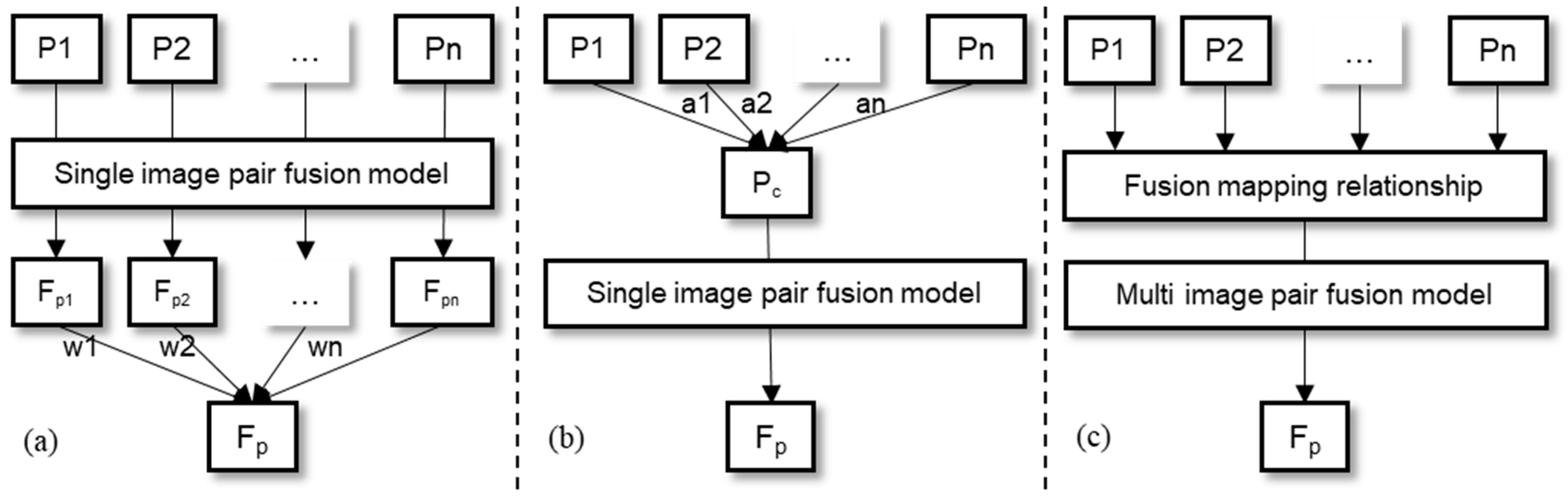
2.3. Fusion Model Structure

LOTSFM is structured with reference to Fit-FC, a spatiotemporal fusion model that explicitly decomposes the structure into regression model fitting (RM), spatial filtering (SF), and residual compensation (RC) [66]. Many spatiotemporal fusion models can identify components similar to those of Fit-FC [67,68,69]. Additionally, the structure of the LOTSFM was adjusted to address the problem of long-time-series fusion for LST. Sensor difference term estimation (SDE) replaces the RC to reduce errors due to significant spatial and temporal variations in the difference term. An additional missing pixel-filling (MPF) component was added to ensure that as many time series as possible were considered for fusion, as shown in Figure 3.
The fusion process of LOTSFM is divided into two stages: training and prediction. The training stage was performed only once to obtain a time-series generic mapping relationship between the coarse and fine image pairs. The prediction stage generated fine images on each prediction date based on the mapping relationship. This is similar to the neural network working process; however, LOTSFM is based on the traditional principle that the training stage constructs mapping relations mainly through regression, which is expected to be faster. LOTSFM is based on time-series generic parameters obtained in the training stage, which are used in the fusion prediction for each date without the need for repeated calculations, thereby improving the efficiency of fusion.

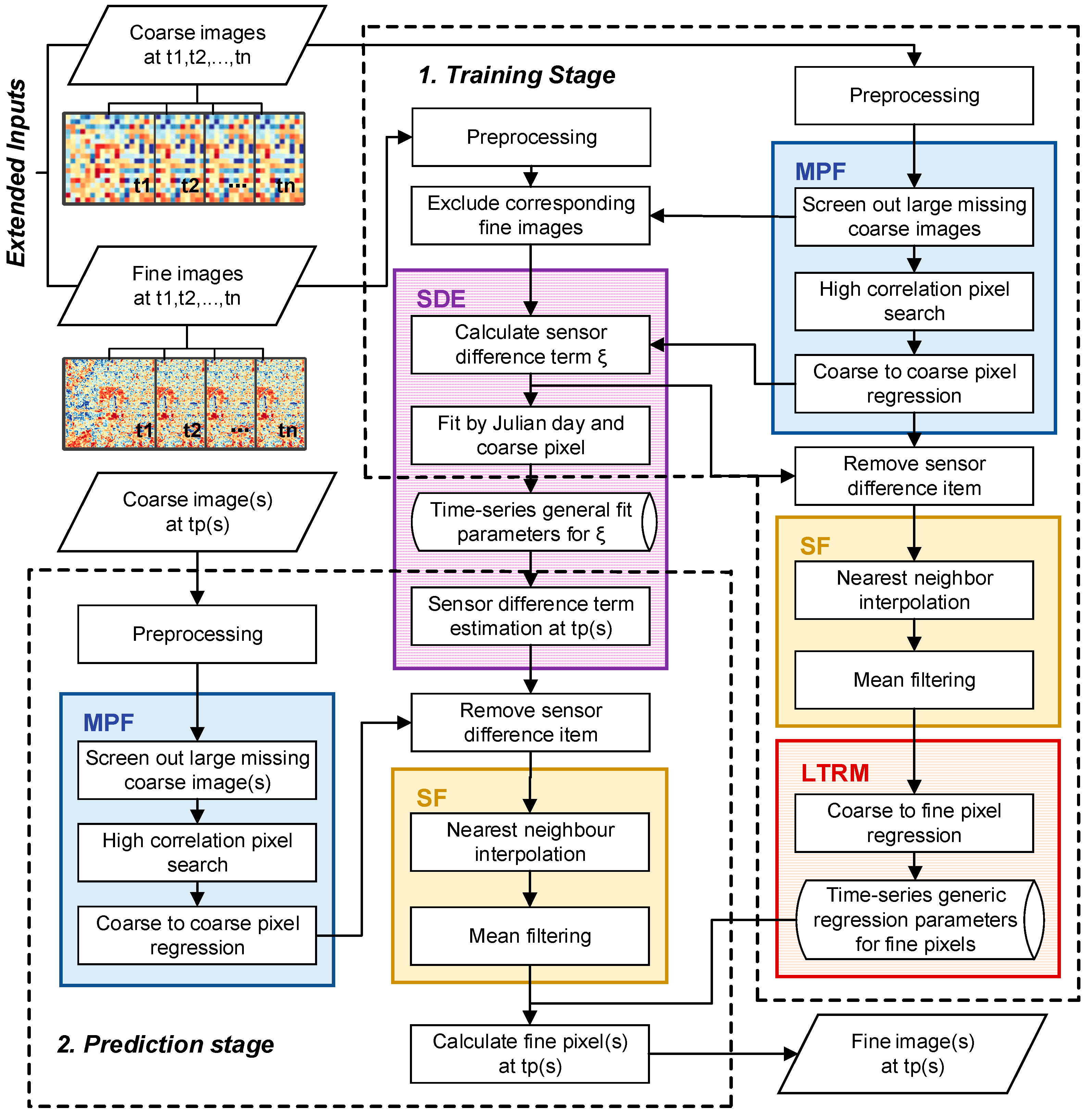
2.4. Long Time-Series Regression Model

For the LST model, it is assumed that there is a high correlation between neighboring fine pixels in the time series. This was based on two considerations. (1) For fine pixels that are sufficiently adjacent, their values should correlate according to the first law of geography [70]. (2) Although abrupt changes such as land cover may occur over time and distance, the LST can still be strongly correlated in the time series due to the heat transfer between adjacent objects and similar conditions of solar thermal radiation. Based on this assumption, it is reasonable to establish the equation between any fine pixels in the neighborhood using coarse pixels as the neighborhood range, which can be described as
F x i k , t = a x i k , x i j F x i j , t + b x i k , x i j + r x i k , x i j , t
where, F ( x i k , t ) and F x i j , t are the LST values of any two fine pixels in the coarse pixel x i at date   t , respectively. a x i k , x i j and b x i k , x i j are coefficients that do not vary with t, r x i k , x i j , t , which is the residual.
According to the pixel-temperature mixing principle [71], the value of the coarse pixel x i , C ( x i , t ) , is equal to the average of the fine pixel values F x i k , t in it plus the ξ term, which can be expressed as:
C x i , t = 1 m k = 1 m F x i k , t + ξ x i , t
where ξ is the bias caused by the observation of different sensors and is referred to as the sensor difference term. Considering that ξ of LST may be significantly different across times and coarse pixel locations, it is set to ξ ( x i , t ) . m is the number of fine pixels within a coarse pixel. From Equations (1) and (2), the pixel relationship between the different scales can be expressed as
C x i , t = F x i j , t · 1 m k = 1 m a x i k , x i j + 1 m k = 1 m b x i k , x i j + 1 m k = 1 m r x i k , x i j , t + ξ x i , t .
Similar to Equation (3), the relationship between the pixels at different scales exhibits linearity. The difference is that the sensor difference term ξ in Equation (5) causes the correlation between pixels at different scales to weaken compared to those of the fine pixels at the same scale. We expect to exclude the effect of the difference term ξ to retain a stronger correlation. Therefore, we set:
C F ( x i , t ) = C ( x i , t ) ξ ( x i , t )
where, C F x i , t is the coarse pixel value for the ideal case in which no observed difference exists between the sensors.
Based on Equations (5) and (6), the relationship between the ideal coarse pixel x i and the contained fine pixel x i j at any date t can be expressed as
F x i j , t = α F x i j C F x i , t + β F x i j + r C F x i j , t
where, α x i j and   β x i j can be estimated using the ordinary least squares method (OLS) [72,73,74]. The residual r x i k , x i j , t between fine pixels, is assumed to be an unpredictable fraction caused by abrupt spatial and temporal variations in land cover that cannot be reduced by a more macroscopic-scale least-squares fit between coarse and fine pixels. Thus, transforming Equation (5),   r C F x i j , t for the predicted residuals is expressed as:
r C F x i j , t = k = 1 m a x i k , x i j 1 · k = 1 m r x i k , x i j , t
Because a x i k , x i j floats around 1, r C F x i j , t is approximated as the regional average of r x i k , x i j , t . Thus, the ideal coarse pixel value C F constructed would have a high correlation with F close to that between the fine pixels and, on average, make the correlation more stable. Therefore, a well-regressed relationship between C F and F is expected.
In contrast to previous temporally dependent spatiotemporal fusion principles [24], LOTSFM generalizes this dependence principle for different locations and long time series according to Equation (5). Specifically, previous temporal dependence principles generally exist between the reference and predicted dates at the same location, and fusion parameters are derived from linear sections of the temporal profile, such as Fit-FC and ESTARFM. The LOTSFM generalizes the linear form applicable to multiple dates (long time series) at different locations. In Section 3.1, the principle is validated based on the fact that pixels at different scales exhibit strong correlations over a long time series.

2.5. Sensor Difference Term Estimation

The sensor difference term is generally regarded as a constant in surface reflectance spatiotemporal fusion models, including classical models such as STARFM and FSDAF. However, the effect of the sensor difference term on the LST fusion problem was significant across time and location, possibly because of data differences. For example, the significant variation of ξ with time and location for the Beijing region is shown in Figure 4. Therefore, the sensor difference term is defined as Equation (9), which varies with the time and location of coarse pixel acquisition, was considered in this study.
C x i , t and J ( t ) are two variables available for estimating the difference term of the sensor. According to earlier studies [42,75], the introduction of temporal variables has the potential to improve spatiotemporal fusion. J ( t )   is the transformation of the date represented by t into a Julian day, with the year discarded to facilitate its introduction into the estimation of the sensor difference term. It can also be regarded as the day of the year (DOY). For example, if t represents 1 August 2017, the corresponding Julian date is 213. We provide the following fit model that can be used for the sensor difference term estimation:
ξ ^ x i , t = α ξ x i C x i , t + β ξ x i + γ ξ x i s i n 2 π 365.25 J t + θ ξ x i
where, α ξ , β ξ , γ ξ and θ ξ are fitting parameters that vary for the location x i of the coarse pixel C x i , t .
The form of the Equation (9) fit is explained as follows: (1) The larger the coarse pixel value C , the more likely it is that a larger ξ appears, showing a certain linear correlation. (2) Jules Day J ( t )   as a date variable: The sinusoidal function is more often used to express periodicity [76]. Furthermore, since the period of the Julian day is fixed, the frequency of the sinusoidal function is known to be 2 π / 365.25 . In Figure 4, estimated values ξ ^ tend to be within the interquartile range (Q3–Q1), demonstrating alignment with the observed variations.

2.6. Missing Pixel Filling

The missing pixel problem limits the use of spatiotemporal fusion models and reduces the spatiotemporal continuity of fused data. Based on the assumptions considered in Section 2.4 for pixel correlation, there should also be a time-series correlation between neighboring coarse pixels. Therefore, a solution to the problem of a limited number of missing pixels occurring in coarse-resolution images on the predicted date can be provided in view of pixel correlation. It is assumed that the level of correlation between coarse pixels is sufficient to fulfill the need for a suitable window range. The correlation between the coarse pixels is described in Section 3.1. The equation for filling any coarse pixels within the search window can be established as follows:
C ^ M P F x u , t p = α x u C x v , t p + β x u ,
x v = arg max x x u   c o r r c o e f ( c ( x ) , c ( x u ) ) .
In Equation (10), C ^ M P F x u , t p is the regression estimate of the missing pixels C x u , t p , and the coefficients α x u and β x u can be solved by OLS. Equation (11) indicates that C x v , t , which is used to establish the regression relationship with C x u , t , is the coarse pixel with the highest time-series correlation.

2.7. Spatial Filtering

The primary cause of blocky artifacts in spatiotemporal fusion is the inconsistency in spatial resolution [67,77]. The raster boundaries of coarse-resolution images are not real land cover boundaries, although they are fused into spatial textures at fine resolution, which causes artifacts [78,79]. Spatial filtering by calculating the spectral differences to find similar pixels is a classic solution to artifact problems [19]. However, the efficiency of the pixel-level search approach is relatively low [24,80], and pure pixels and classification principles may not be suitable for continuous LST data [63].
Inspired by the All-around Performance Assessment (APA) framework [81], a fused image is considered to contain spectral and spatial information. The coarse-resolution image on the predicted date provides overall spectral information, whereas the fine-resolution image on the reference date provides detailed spatial information that is not provided by the coarse image. Therefore, we consider spatial filtering of coarse images to weaken the coarse spatial resolution spatial information as much as possible so that more fine-resolution image spatial information is inherited to suppress the appearance of artifacts. Specifically, the coarse resolution image is sampled to fine resolution based on nearest neighbor interpolation. The blocky texture caused by the coarse raster is removed based on mean filtering and then fed to the fuser as a normal coarse image.

3. Experiments and Results

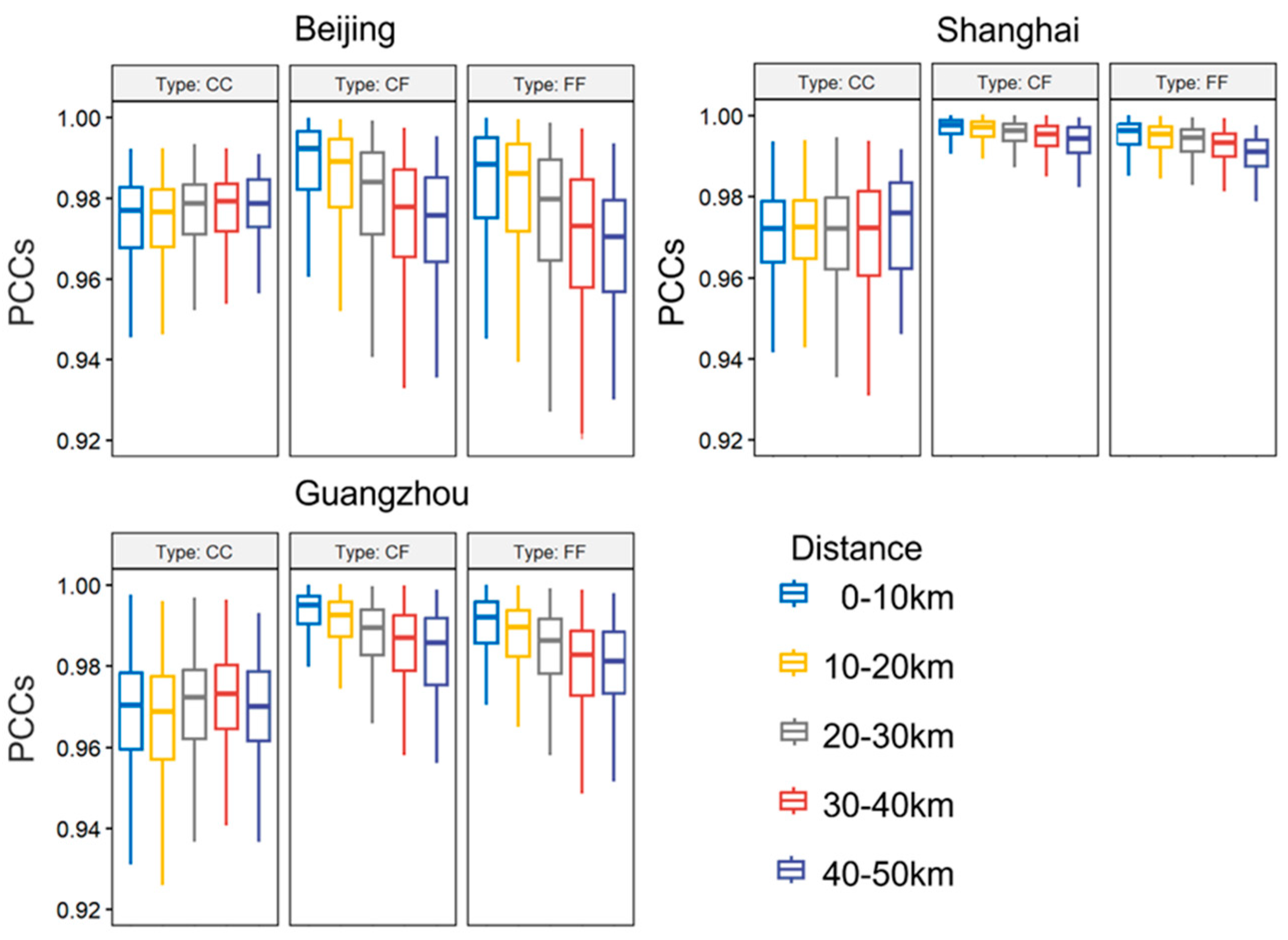
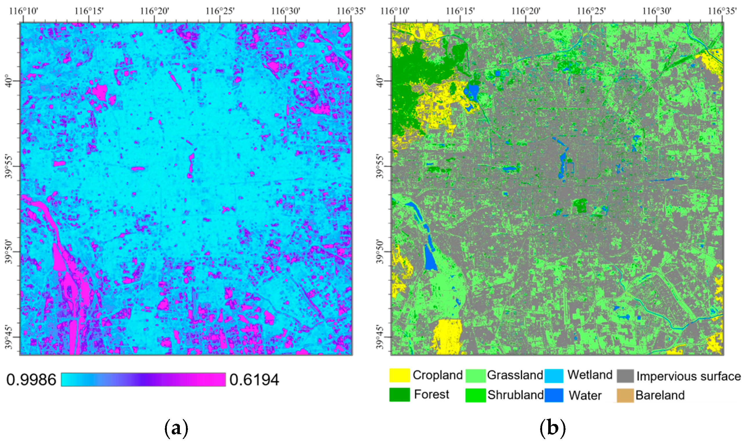
3.1. Time-Series Correlation Levels between Pixels

Correlation statistics for the study regions can corroborate the principal assumption [82] and help anticipate the fusion performance of the LOTSFM. Correlations among coarse pixels, ideal coarse pixels, and fine pixels were assumed to construct LOTSFM. Therefore, we verified the variations in these three types of correlations using the Euclidean distance from the center of the pixel. In each region, 20,000 samples were taken for each type of correlation, and the distances were discretized to form Figure 5.
The average correlation for all types in the regions was greater than 0.95, which is in line with the principal assumption of high correlations between adjacent pixels. The correlations between coarse pixels (CC) were largely stable with distance over the experimental region range; therefore, the search window for missing pixel filling was set to be region global. The correlation between the ideal coarse pixels and fine pixels (CF) and between fine pixels (FF) decreases with distance similarly, which conforms to the expectation of ideal coarse pixels in principle, i.e., to retain the stronger correlation by excluding the difference term ξ .

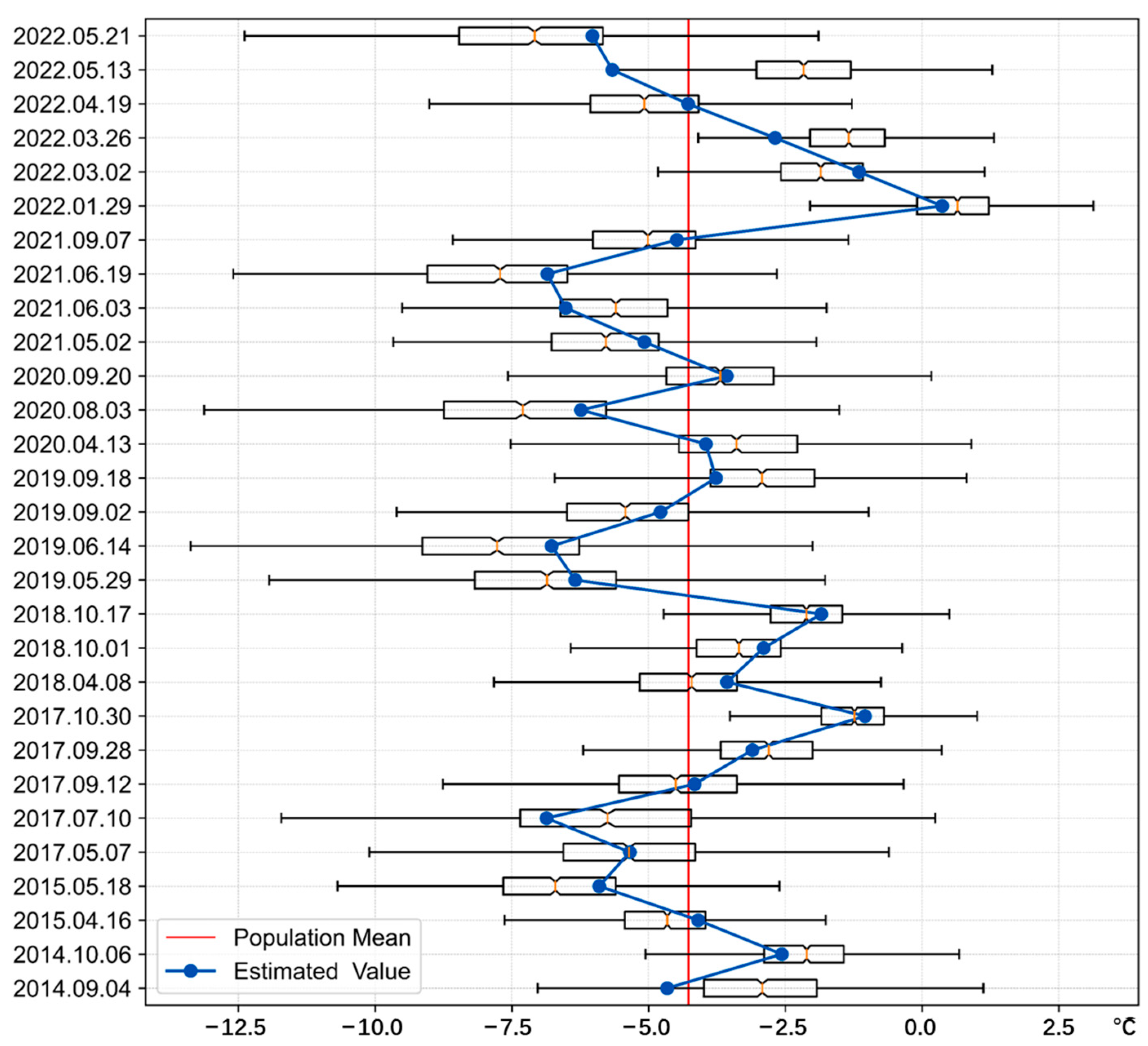
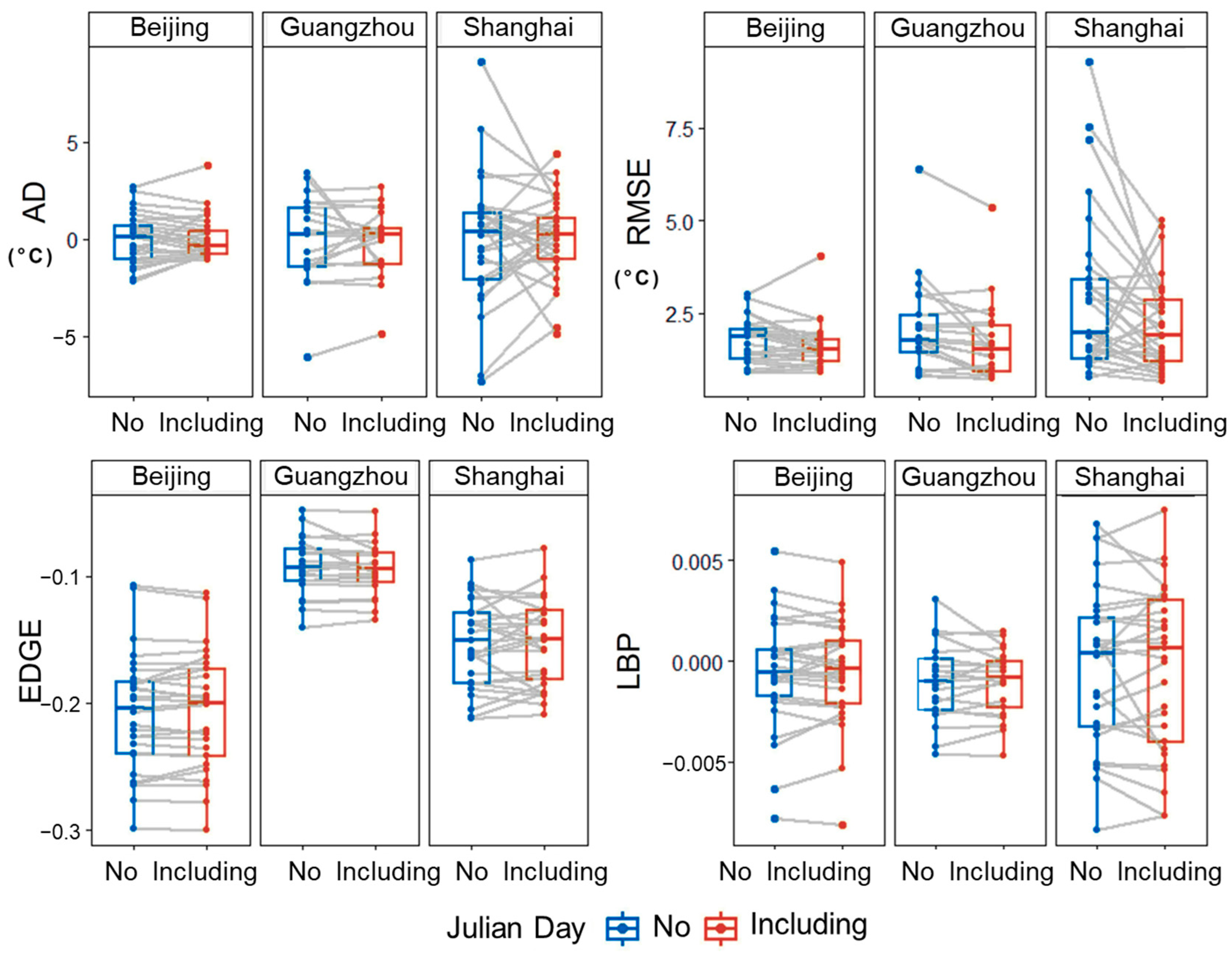
3.2. Regional Replicability Assessment of LOTSFM

The LOTSFM fusion accuracy experiments were conducted in Beijing, Shanghai, and Guangzhou, China. Due to the small dataset size of the fusion, leave-one-out cross-validation (LOOCV) was considered appropriate, enabling as many rounds of validation as possible. LOOCV avoids randomness in the division of training and validation samples so that the accuracy estimates for a given dataset are constant and objective [83]. LOOCV was performed by removing one image pair at a time for validation and feeding the remaining data into the training set.
Accuracy is assessed with reference to the all-round performance assessment (APA) [81], which provides a comprehensive and standard model assessment framework adopted by new spatiotemporal fusion models, such as variation-based spatiotemporal data fusion (VSDF) [69] and the comprehensive flexible spatiotemporal data fusion (CFSDAF) [63]. Specifically, the APA proposes using metrics including the average difference (AD), root-mean-square error (RMSE), Robert’s edge (EDGE), and local binary patterns (LBP) as evaluation criteria for assessing the performance of spatiotemporal fusion algorithms.
Based on the data in Table 2, Beijing, Shanghai, and Guangzhou conducted 29, 29, and 21 rounds of validation, respectively. The results of each round are shown in Tables S1–S3 in the Supplementary Materials, and the statistics are summarized in Table 3.
In the three-region experiment, the lowest absolute average AD value is 0.006 °C in Beijing, and the highest is about 0.13 °C in Guangzhou. The small average AD results for the three regions suggest that LOTSFM provides an approximately unbiased estimate for overall long time-series samples. The minimum RMSE is in Beijing, 1.60 °C, and the maximum is in Shanghai, 2.17 °C.

3.3. SDE Component Validity Assessment of LOTSFM

To verify the validity of the introduction of the Julian day for the estimation of the sensor difference term, we also conducted LOOCV for each region of LOTSFM without the Julian day input. The results of each round are shown in Tables S4–S6, and the statistics are summarized in Table S7 in the Supplementary Materials.
To provide a more visual representation of the optimization in each round, Figure 6 shows the results based on paired box plots. The AD of each region showed a decrease in variance; the values were more concentrated at approximately 0. The RMSE exhibited a significant decrease in the average value (p < 0.05). The introduction of Julian days does not include additional spatial information; therefore, the EDGE and LBP indicators, which are related to spatial detail, did not show significant changes.
The three-city fusion images obtained from the cross-validation experiments are shown in Figure 7. Despite the significant difference in resolution between MODIS (1 km) and Landsat (30 m), the LOTSFM algorithm can produce fused images with spatial details similar to those of Landsat using MODIS data from the predicted data. Although Figure 7 displays only thumbnail images, the thermal environment textures within the city, such as rivers, are visible in the Landsat and LOTSFM fusion images. In contrast, MODIS provides coarse information on the distribution of urban temperatures. This highlights the critical need to obtain high-resolution temperature data through spatiotemporal fusion for investigating urban thermal environments.

3.4. Fusion Accuracy Comparison with Other Models

To assess the LOTSFM fusion capability, STARFM, ESTARFM, FSDAF, and GAN-STFM were selected for comparison experiments, all of which are classical and easily accessible from open sources. STARFM, the earliest and most widely used spatiotemporal fusion model, is often used as a standard model for comparison [41,44,84]. ESTARFM is an enhanced version of STARFM, which has been used in many LST fusion studies [40,85]. FSDAF, as a hybrid fusion model, combines the strengths of weight function-based and unmixing-based methods and has achieved relatively good results in some fusion comparison experiments [86,87]. GAN-STFM [56] is a deep-learning fusion method that uses a classical generative adversarial network (GAN). GAN-STFM has a fusion process similar to that of LOTSFM, which involves training and prediction and is therefore used for comparison experiments.
A comparative experiment based on the Beijing region was conducted using four randomly selected image pairs for independent validation. The dates selected were 7 May 2017, 8 April 2018, 2 September 2019, and 29 January 2022. Based on the principle of the nearest date input and the respective model input requirements, STARFM and FSDAF use the nearest one-date image pair, whereas ESTARFM uses the nearest two-date image pairs as the fusion input. The GAN-STFM model allows as many image pairs as possible to be used for training; therefore, LOTSFM uses the rest of the 25 dates image pair as input.
The experimental accuracy results are visualized using the APA diagrams in Figure 8, and the results of the accuracy parameters are listed in Table 4. In the APA diagram, the closer to the center of the semicircle, the better the RMSE accuracy, and the closer to the central axis, the better the spatial detail, using different colors to indicate the AD. The APA delineated green areas of good and grey areas of fairness based on the input to visually evaluate the fusion performance. The fair area indicates that the fused image is better than the input image in one of the spectral or spatial accuracy aspects, and a good area is better in both aspects. In Figure 8, ESTARFM and LOTSFM are categorized as good in (b) and (c). The contemporaneous optimal accuracy values are listed in Table 4, with 10 optimal values for LOTSFM, 6 for ESTARFM, and 1 for FSDAF. ESTARFM and LOTSFM were outstanding in the experiments; however, LOTSFM was more robust. In (d), the ESTARFM error is large, and LOTSFM is still able to maintain stable accuracy.

3.5. Fusion Time Comparison with Other Models

The fusion time consumption records for each model are listed in Table 5. The three models, STARFM, ESTARFM, and FSDAF, undergo a complete fusion process each time, and the process parameters are not time-series generic. For comparison purposes, the total time consumption was noted as the prediction process consumption. Contrastingly, the GAN-STFM and LOTSFM are divided into two stages: training and prediction. The GAN-STFM time-series generic parameters are mainly neuron weights, and the LOTSFM are regression parameters.
The experimental workstation was configured with an Intel(R) Xeon(R) Silver 4110 CPU, NVIDIA Quadro P4000 GPU, and Linux system environment. STARFM, ESTARFM, FSDAF, and LOTSFM use the CPU for fusion calculations. Additionally, based on the features of LOTSFM, in which each pixel can be processed independently, multiple processes can be used to improve the fusion efficiency in the training stage. Depending on CPU performance, we used 12 processes for the experiments. The GAN-STFM model was trained for 500 iterations on a GPU, as described in a previous study [56]. According to the results in Table 5, STARFM is the least time-consuming model, 141 s, if the fusion is only performed for a certain date. LOTSFM requires a training process and is second only to STARFM in terms of time consumption, which is 248 s. When conducting multi-date experiments, LOTSFM and GAN-STFM only performed the prediction process based on the first training parameters, consuming less than 1 s.

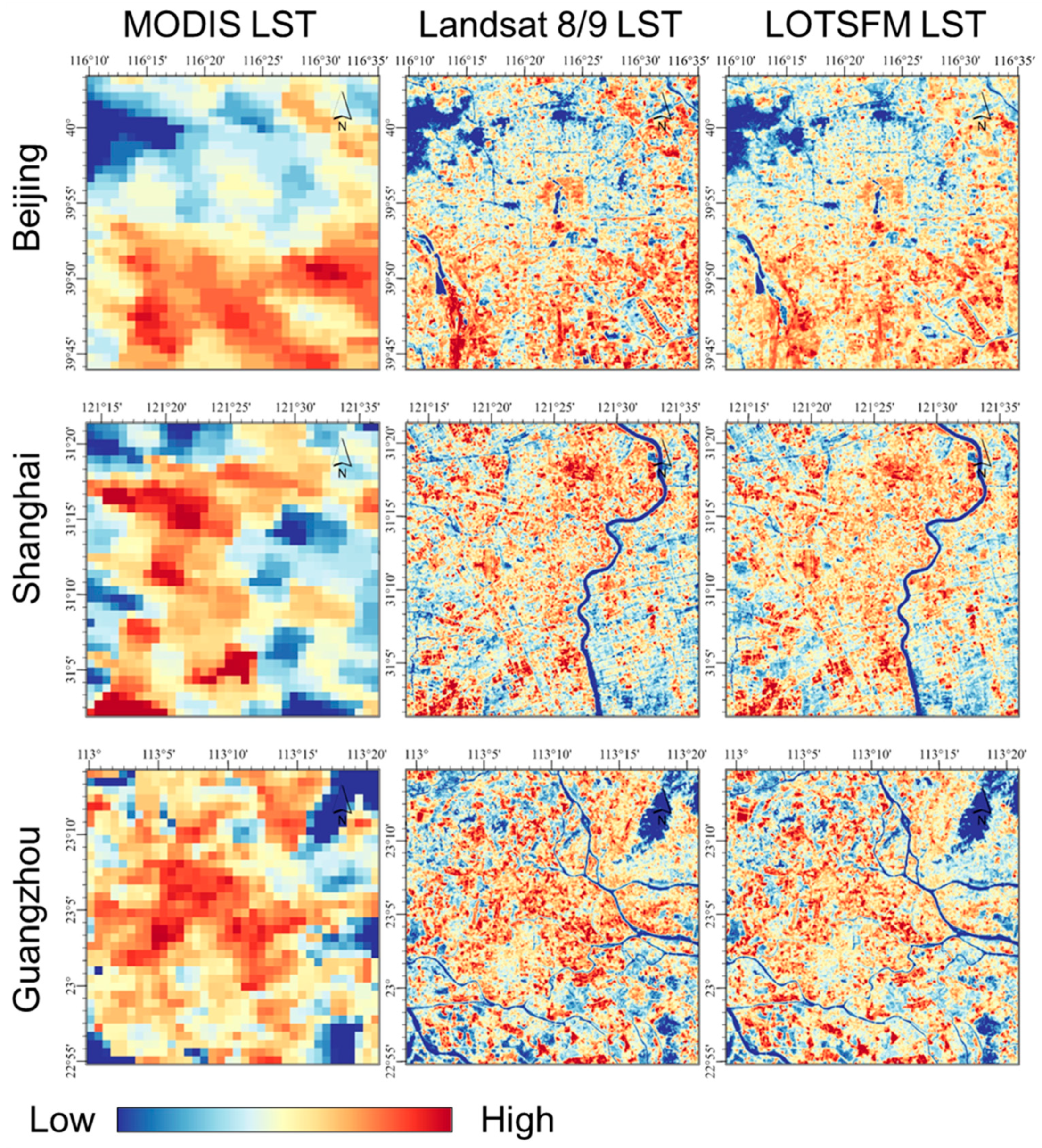
3.6. Spatial Details Comparison with Other Models

A representative LST fusion experimental zone in Beijing was selected to compare the spatial details of each model, as shown in Figure 9. Summer Palace was a royal garden of the Qing Dynasty. The lake area in the Summer Palace is divided into three small lakes by an embankment: Kunming Hu 1, Kunming Hu 2, and Tuancheng Hu. Each of the three water surfaces comprised an island in the center of the lake, which appeared as an approximately circular normal-temperature region. The complex landscape and distinct temperature distribution in this area were used as contrasts for spatial details.
In Figure 9, image noise was observed in the FSDAF image, which is consistent with that in earlier studies that used FSDAF for LST fusion [63]. The GAN-STFM images exhibited excessive smoothness, which may be due to LST data differences, despite the use of multiscale structural similarity (MS-SSIM) to ensure visual performance. LOTSFM is intuitively the closest to Landsat, particularly in terms of the distribution of water LST in the Kunming Hu 2.
The spatial distribution of hot and cold urban areas is of concern for guiding the mitigation of thermal risks [88,89]. Therefore, representative areas with cooling effects, such as water bodies and green spaces, are selected in Figure 10 to reflect the detailed performance of each model in hot and cold areas.
Figure 10 Area 1 provides a detailed spatial representation of the lake area near the Summer Palace. Among the models, the LOTSFM low-temperature area demonstrates a better fit to the lake boundary. Moreover, the Tuancheng Hu Lake in the upper left stands out due to its relatively smaller area, resulting in a weaker cooling effect. As a result, the surface temperature of this lake does not exhibit the same deep blue hue as the other lake areas. Figure 10 Area 2 depicts a slanted square-shaped water body with a small land patch at its center. However, the models other than LOTSFM do not display the surface temperature of the central land area. Figure 10 Area 3 showcases the Forbidden City, where LOTSFM performs clearly in representing the cold area within the square-shaped moat. Figure 10 Area 4 represents the Temple of Heaven, which is predominantly covered in greenery, with two bare circular building areas clearly depicted in the LST of LOTSFM.

3.7. Error Distribution of Different Input Models

Because images with close dates have minimal land cover changes, they are generally used as reference image pairs for input; this principle was used for the experiments in Section 3.5. However, large differences in the values of the images with the closest dates among those that can be collected may also exist. The green and grey areas in the APA diagram reflect the reference image pair information. The large difference between the grey and green areas in Figure 8d is due to the excessive difference between the values of the reference pair and the predicted image, even though the reference and predicted dates were closest to each other in the sample dataset.
The extended input is intended to allow the model to synthesize the input data by feeding sufficient pairs of images to avoid artificial selection. Furthermore, more data input increases the upper limit of what can be achieved through fusion. Both STARFM and FSDAF achieved similar results when using a single image-pair input, as shown in Figure 11. ESTARFM, GAN-STFM, and LOTSFM expand the inputs. However, the expansion of ESTARFM is limited. Although it achieves good results in Figure 11 on 2019.09.02, the result on 2022.01.29 is unsatisfactory, indicating that its robustness still needs improvement. GAN-STFM showed ideal absolute difference distribution results for the two fusions on 2019.09.02 and 2022.01.29 in Figure 11, while LOTSFM performed relatively ideal on all dates.
Having a sufficient sample input is advantageous for learning-based methods; however, the fused reference image pairs that can currently be prepared for deep learning methods are still small datasets. The black-box approach used for small datasets can lead to high uncertainty in the fusion results. For instance, in Figure 11, the GAN-STFM shows concentrated image prediction errors in the middle of the region on 2017.05.07, while the other models have fused image errors that are low in the middle and high around the region. Furthermore, a small block artifact is visible in the upper left corner of the GAN-STFM result for 2022.01.29, while the other date images show no significant artifacts.

4. Discussion

4.1. Usage and Data Flexibility

In the experiments, the 36 km by 36 km area used was able to cover the main regions of the megacity. LOTSFM performs fusion in coarse pixels such that the fusion of larger or tiny areas is also easily achieved while allowing parallel computing to be easily applied to increase the speed of fusion. Based on the training and prediction processes, this allows potentially repetitive parameter calculation processes to be combined, with each subsequent fusion requiring only short prediction processes. This reduces the average computational time for multi-date fusion, enabling batch spatiotemporal fusion. The high spatial and temporal continuous LST remote sensing data generated have the potential to study urban thermal environment dynamics. For example, in industrial areas, it can be used to judge the intensity of work and monitor industrial thermal anomalies and pollution that may occur on any date. MODIS data do not accurately capture factory buildings, and Landsat data may suffer from a lack of key data. Based on the fused data available in the batch, the fine monitoring of industrial heat at a daily frequency can be achieved.
Additionally, the LOTSFM can accommodate the LST from different sensor sources. This is because (1) in Section 2.1, the coarse-resolution data used MOD11A1 and MYD11A1 from two different satellites, Terra and Aqua, respectively. Therefore, it is reasonable to believe that LOTSFM supports the fusion of other satellite LST data, such as FY-3C, ASTER, and Sentinel3. (2) In Section 3.1, even for the longest distance tested (40–50 km), a high correlation between ideal coarse pixels and fine pixels was observed (average PCCs > 0.95). Although MODIS and Landsat have coarse and fine resolutions of 1 km and 30 m, respectively, fusion with higher resolution ratios is still possible with the support of high correlation.

4.2. Fusion Performance Predictability

Based on the correlation results between the coarse and fine pixels during training, LOTSFM can predict the fused performance at different locations to reduce uncertainties. Figure 12a shows the spatial distribution of ideal correlations between the coarse and fine pixels during the training process, with high correlations in the middle of the region and low correlations around it. This is consistent with the absolute difference distribution of LOTSFM in Figure 11, particularly the results for 7 May 2017. Furthermore, based on the assumption of LOTSFM, heat transfer helps maintain stable temperature correlations between ground objects by promoting a temperature balance towards homogeneous conditions. However, the temperature of objects with high specific heat capacity is less affected by heat transfer, inhibiting its enhancement effect on the temperature correlation. Figure 12b shows a 10 m resolution land cover image of Beijing in 2017 derived from the FROM-GLC10 dataset [90]. Based on the heat transfer hypothesis of the LOTSFM, it is possible to explain the reason why the impermeable water areas with a low specific heat capacity in Figure 12b are more likely to have a high correlation and low absolute difference than the water areas.
Based on the 29 image pairs prepared for this study in Beijing, Figure 13 provides a time-series analysis of the potential influences of land cover. Figure 13a shows the time-series variations of LST for each land cover class. Distinct temperature differences exist among different land cover classes. The temperature ranks from high to low as follows: impervious surface, grassland, cropland, forest, and water bodies. While the average absolute difference (AAD) for different land cover types in Figure 13b is not highly stable along the time series, a more distinct observation can be performed by examining the box plot in Figure 13c, revealing that water bodies exhibit significantly higher AAD values and greater dispersion compared to impervious surfaces. This observation is consistent with the spatial patterns shown in Figure 12, indicating that LOTSFM has different absolute differences in fusion for different land cover classes. Based on this characteristic, it can be anticipated that LOTSFM is well-suited for monitoring thermal dynamics in urban areas characterized by the aggregation of impervious surfaces.
Furthermore, in Figure 13a, the lowest LST is observed on 2022.01.29, and the fusion AAD still exhibits favorable performance. This indicates that even under extreme temperature conditions, LOTSFM is capable of achieving stable predictions based on expanded inputs. However, in Figure 13b, a relatively large AAD is observed on 2022.05.13, which cannot be explained by land cover or correlations. Sensor differences may be the dominant factor contributing to this observation.
It should be recognized that spatial and temporal distribution of absolute differences did not completely correspond to the correlation distribution or land cover, and it was necessary to focus on the deviations caused by sensor differences. Earlier studies considered sensor differences, including bandwidth and solar geometry factors, to be constant [19,35]. In reflectance fusion, such considerations may already be justified because reflectance is relatively constant throughout the day. However, LST varies significantly throughout the day, and sensor observations may not be taken simultaneously, even on the same day. Treating the sensor difference term as a constant can lead to large deviations, which the LOTSFM considers. This is a potential reason for the performance drop in classical reflectance models when temperature–data fusion is conducted.

4.3. Limitations

LOTSFM is built upon the correlation of pixel time series. Insufficient input samples or poor correlation conditions can limit the performance of LOTSFM. In this case, the minimum input model may be the better choice. Therefore, the integration of minimum input models to form hybrid complementarities is prospected. Additionally, some minimum input models sensible to changes in ground cover are ideal for integration to address the difficulties in capturing land-cover changes.
Missing pixel filling in LOTSFM only serves to make the image meet the input integrity requirements. It is not discussed and validated in as much detail as a dedicated cloud missing reconstruction algorithm. Moreover, as with most temporal reconstruction algorithms, cloud filling in LOTSFM can only provide assumed LST values based on cloud-free conditions. Recent studies, such as the research conducted by Gong et al. [91], have proposed a reconstruction method using a nonlocality-reinforced network (NRN), examined various combinations of multimodal datasets, and evaluated them, which provides a useful reference for enhancing the missing pixel filling component of LOTSFM. Moreover, microwave data (e.g., FY-3D MWRI) is expected as input for LOTSFM to reconstruct missing pixel values closer to the real cloud conditions in the future.
The expansion of inputs in LOTSFM remains limited. We believe that a more comprehensive form of input expansion should encompass not only an increase in time series but also the incorporation of data from multiple sources. Currently, most spatiotemporal fusion models predominantly focus on space-based satellite data. Aerial data holds significant potential for integration into spatiotemporal fusion methods, especially given the rapid development of aerial unmanned drone technology. The fusion of aerial and satellite data can lead to the generation of higher-resolution and more accurate data, which has already been used for monitoring soil, crops, and forests [92,93,94]. However, while the integration of aerial data into surface temperature fusion is not yet widespread, it does not detract from recognizing it as one of the promising research directions.

5. Conclusions

High spatiotemporal resolution LST data are crucial for urban thermal environment studies; however, they are not always readily available or generated. Spatiotemporal fusion presents a potential solution; however, practical production applications face several challenges, including difficulties in sample selection, handling cloud cover, and fusion speed. Based on the above issues, a spatiotemporal fusion model, LOTSFM, based on long time-series data was proposed. The main contents and model features are summarized as follows:
  • LOTSFM is a model with extended inputs, requiring only the necessary number of input samples to avoid sample selection and improve the robustness of the results.
  • LOTSFM consists of two stages, training and prediction, and employs multi-process parallel computing to rapidly generate spatiotemporal fusion data in batches.
  • LOTSFM utilized Julian days to estimate the sensor difference term, which was experimentally shown to significantly improve numerical accuracy.
Based on Landsat 8/9 and MODIS LST data, 79 image pairs were collected from three cities. The cross-validation results show that the average RMSE values are 1.60 °C, 2.17 °C, and 1.72 °C for Beijing, Shanghai, and Guangzhou, respectively. This capability enables effective monitoring of dynamic changes in urban heat island intensity, industrial heat emissions, and residential heat exposure. Particularly in the current global climate instability context, LOTSFM holds great potential in offering valuable guidance for proactively addressing and mitigating the detrimental impacts associated with extreme heat.
Nevertheless, it is important to acknowledge that further enhancements are required for LOTSFM. For instance, the fusion accuracy in areas with low correlation may be relatively diminished. To address this limitation, future research could explore the integration of alternative spatiotemporal fusion models to establish a complementary relationship, thereby enhancing the fusion accuracy in such areas. Conclusively, more than just the fusion of data, the complementary fusion of models will potentially be an important trend in the development of spatiotemporal fusion.

Supplementary Materials

The following supporting information can be downloaded at: https://www.mdpi.com/article/10.3390/rs15215211/s1, Table S1/S2/S3: Beijing/Shanghai/Guangzhou regional LOTSFM leave-one-out cross-validation results; Table S4/S5/S6: Beijing/Shanghai/ Guangzhou regional LOTSFM leave-one-out cross-validation results without Julian day input; Table S7: Summary statistics of LOOCV results for each region of LOTSFM without Julian day input; Table S8. Figure 7 Setting of color bar values for each image type in each region.

Author Contributions

Conceptualization, S.C.; methodology, S.C. and Q.M.; software, S.C. and J.Q.; validation, S.C., L.Z. and X.H.; formal analysis, S.C.; investigation, S.C.; resources, Q.M.; data curation, L.Z.; writing—original draft preparation, S.C.; writing—review and editing, L.Z., J.Q., J.G. and Q.M.; visualization, S.C.; supervision, L.Z.; project administration, L.Z., X.H. and Q.M.; funding acquisition, Q.M. All authors have read and agreed to the published version of the manuscript.

Funding

This research was funded by the National Natural Science Foundation of China (42201384), FY-3 Lot 03 Meteorological Satellite Engineering Ground Application System Ecological Monitoring and Assessment Application Project (Phase I): ZQC-R22227, and Youth Innovation Promotion Association CAS (2023139).

Data Availability Statement

Landsat 8/9 OLI_TIRS Collection 2 Level-2 product data covering the study area can be obtained from the United States Geological Survey (USGS, http://glovis.usgs.gov/ (accessed on 6 February 2023)). Daily MOD11A1 and MYD11A1 data covering the study area can be obtained from NASA (http://ladsweb.nascom.nasa.gov/ (accessed on 8 February 2023)).

Conflicts of Interest

The authors declare that they have no known competing financial interests or personal relationships that could have appeared to influence the work reported in this paper.

References

  1. Peng, S.; Piao, S.; Ciais, P.; Friedlingstein, P.; Ottle, C.; Bréon, F.M.; Nan, H.; Zhou, L.; Myneni, R.B. Surface urban heat island across 419 global big cities. Environ. Sci. Technol. 2012, 46, 696–703. [Google Scholar] [CrossRef]
  2. Santamouris, M. On the energy impact of urban heat island and global warming on buildings. Energy Build. 2014, 82, 100–113. [Google Scholar] [CrossRef]
  3. Singh, N.; Singh, S.; Mall, R. Urban Ecology and Human Health: Implications of Urban Heat Island, Air Pollution and Climate Change Nexus. In Urban Ecology; Elsevier: Amsterdam, The Netherlands, 2020; pp. 317–334. [Google Scholar] [CrossRef]
  4. Zhou, D.; Zhao, S.; Zhang, L.; Sun, G.; Liu, Y. The footprint of urban heat island effect in China. Sci. Rep. 2015, 5, 11160. [Google Scholar] [CrossRef]
  5. Meng, Q.; Zhang, L.; Sun, Z.; Meng, F.; Wang, L.; Sun, Y. Characterizing spatial and temporal trends of surface urban heat island effect in an urban main built-up area: A 12-year case study in Beijing, China. Remote Sens. Environ. 2018, 204, 826–837. [Google Scholar] [CrossRef]
  6. Ghaderpour, E.; Mazzanti, P.; Mugnozza, G.S.; Bozzano, F. Coherency and phase delay analyses between land cover and climate across Italy via the least-squares wavelet software. Int. J. Appl. Earth Obs. Geoinf. 2023, 118, 103241. [Google Scholar] [CrossRef]
  7. Liu, J.; Hagan, D.F.; Liu, Y. Global Land Surface Temperature Change (2003–2017) and Its Relationship with Climate Drivers: AIRS, MODIS, and ERA5-Land Based Analysis. Remote Sens. 2021, 13, 44. [Google Scholar] [CrossRef]
  8. Guan, Y.; Quan, J.; Ma, T.; Cao, S.; Xu, C.; Guo, J. Identifying Major Diurnal Patterns and Drivers of Surface Urban Heat Island Intensities across Local Climate Zones. Remote Sens. 2023, 15, 5061. [Google Scholar] [CrossRef]
  9. Sobrino, J.; Oltra-Carrió, R.; Sòria, G.; Bianchi, R.; Paganini, M. Impact of spatial resolution and satellite overpass time on evaluation of the surface urban heat island effects. Remote Sens. Environ. 2012, 117, 50–56. [Google Scholar] [CrossRef]
  10. Gao, J.; Meng, Q.; Zhang, L.; Hu, D. How does the ambient environment respond to the industrial heat island effects? An innovative and comprehensive methodological paradigm for quantifying the varied cooling effects of different landscapes. GIsci. Remote Sens. 2022, 59, 1643–1659. [Google Scholar] [CrossRef]
  11. Shen, H.; Huang, L.; Zhang, L.; Wu, P.; Zeng, C. Long-term and fine-scale satellite monitoring of the urban heat island effect by the fusion of multi-temporal and multi-sensor remote sensed data: A 26-year case study of the city of Wuhan in China. Remote Sens. Environ. 2016, 172, 109–125. [Google Scholar] [CrossRef]
  12. Meng, Q.; Hu, D.; Zhang, Y.; Chen, X.; Zhang, L.; Wang, Z. Do industrial parks generate intra-heat island effects in cities? New evidence, quantitative methods, and contributing factors from a spatiotemporal analysis of top steel plants in China. Environ. Pollut. 2022, 292, 118383. [Google Scholar] [CrossRef]
  13. Meng, Q.; Liu, W.; Zhang, L.; Allam, M.; Bi, Y.; Hu, X.; Gao, J.; Hu, D.; Jancsó, T. Relationships between Land Surface Temperatures and Neighboring Environment in Highly Urbanized Areas: Seasonal and Scale Effects Analyses of Beijing, China. Remote Sens. 2022, 14, 4340. [Google Scholar] [CrossRef]
  14. Kovalskyy, V.; Roy, D.P. The global availability of Landsat 5 TM and Landsat 7 ETM+ land surface observations and implications for global 30 m Landsat data product generation. Remote Sens. Environ. 2013, 130, 280–293. [Google Scholar] [CrossRef]
  15. Li, J.; Chen, B. Global revisit interval analysis of Landsat-8-9 and Sentinel-2a-2b data for terrestrial monitoring. Sensors 2020, 20, 6631. [Google Scholar] [CrossRef] [PubMed]
  16. Zhu, Z.; Woodcock, C.E.; Holden, C.; Yang, Z. Generating synthetic Landsat images based on all available Landsat data: Predicting Landsat surface reflectance at any given time. Remote Sens. Environ. 2015, 162, 67–83. [Google Scholar] [CrossRef]
  17. Lai, J.; Zhan, W.; Huang, F.; Voogt, J.; Bechtel, B.; Allen, M.; Peng, S.; Hong, F.; Liu, Y.; Du, P. Identification of typical diurnal patterns for clear-sky climatology of surface urban heat islands. Remote Sens. Environ. 2018, 217, 203–220. [Google Scholar] [CrossRef]
  18. Li, J.; Li, Z.-L.; Wu, H.; You, N. Trend, seasonality, and abrupt change detection method for land surface temperature time-series analysis: Evaluation and improvement. Remote Sens. Environ. 2022, 280, 113222. [Google Scholar] [CrossRef]
  19. Gao, F.; Masek, J.; Schwaller, M.; Hall, F. On the blending of the Landsat and MODIS surface reflectance: Predicting daily Landsat surface reflectance. IEEE Trans. Geosci. Remote Sens. 2006, 44, 2207–2218. [Google Scholar] [CrossRef]
  20. Hilker, T.; Wulder, M.A.; Coops, N.C.; Linke, J.; McDermid, G.; Masek, J.G.; Gao, F.; White, J.C. A new data fusion model for high spatial- and temporal-resolution mapping of forest disturbance based on Landsat and MODIS. Remote Sens. Environ. 2009, 113, 1613–1627. [Google Scholar] [CrossRef]
  21. Rao, C.V.; Malleswara Rao, J.; Senthil Kumar, A.; Dadhwal, V.K. Fast spatiotemporal data fusion: Merging LISS III with AWiFS sensor data. Int. J. Remote Sens. 2014, 35, 8323–8344. [Google Scholar] [CrossRef]
  22. Wang, Q.; Blackburn, G.A.; Onojeghuo, A.O.; Dash, J.; Zhou, L.; Zhang, Y.; Atkinson, P.M. Fusion of Landsat 8 OLI and Sentinel-2 MSI Data. IEEE Trans. Geosci. Remote Sens. 2017, 55, 3885–3899. [Google Scholar] [CrossRef]
  23. Zhu, X.; Chen, J.; Gao, F.; Chen, X.; Masek, J.G. An enhanced spatial and temporal adaptive reflectance fusion model for complex heterogeneous regions. Remote Sens. Environ. 2010, 114, 2610–2623. [Google Scholar] [CrossRef]
  24. Zhu, X.; Cai, F.; Tian, J.; Williams, T. Spatiotemporal Fusion of Multisource Remote Sensing Data: Literature Survey, Taxonomy, Principles, Applications, and Future Directions. Remote Sens. 2018, 10, 527. [Google Scholar] [CrossRef]
  25. Wu, P.; Yin, Z.; Zeng, C.; Duan, S.-B.; Gottsche, F.-M.; Ma, X.; Li, X.; Yang, H.; Shen, H. Spatially Continuous and High-Resolution Land Surface Temperature Product Generation: A review of reconstruction and spatiotemporal fusion techniques. IEEE Geosci. Remote Sens. Mag. 2021, 9, 112–137. [Google Scholar] [CrossRef]
  26. Wu, M.; Niu, Z.; Wang, C.; Wu, C.; Wang, L. Use of MODIS and Landsat time series data to generate high-resolution temporal synthetic Landsat data using a spatial and temporal reflectance fusion model. J. Appl. Remote Sens. 2012, 6, 063507. [Google Scholar] [CrossRef]
  27. Zhukov, B.; Oertel, D.; Lanzl, F.; Reinhackel, G. Unmixing-based multisensor multiresolution image fusion. IEEE Trans. Geosci. Remote Sens. 1999, 37, 1212–1226. [Google Scholar] [CrossRef]
  28. Li, A.; Bo, Y.; Zhu, Y.; Guo, P.; Bi, J.; He, Y. Blending multi-resolution satellite sea surface temperature (SST) products using Bayesian maximum entropy method. Remote Sens. Environ. 2013, 135, 52–63. [Google Scholar] [CrossRef]
  29. Xue, J.; Leung, Y.; Fung, T. A Bayesian Data Fusion Approach to Spatio-Temporal Fusion of Remotely Sensed Images. Remote Sens. 2017, 9, 1310. [Google Scholar] [CrossRef]
  30. Cai, J.; Huang, B.; Fung, T. Progressive spatiotemporal image fusion with deep neural networks. Int. J. Appl. Earth Obs. Geoinf. 2022, 108, 102745. [Google Scholar] [CrossRef]
  31. Huang, B.; Song, H. Spatiotemporal Reflectance Fusion via Sparse Representation. IEEE Trans. Geosci. Remote Sens. 2012, 50, 3707–3716. [Google Scholar] [CrossRef]
  32. Zhu, Z.; Tao, Y.; Luo, X. HCNNet: A Hybrid Convolutional Neural Network for Spatiotemporal Image Fusion. IEEE Trans. Geosci. Remote Sens. 2022, 60, 1–16. [Google Scholar] [CrossRef]
  33. Gevaert, C.M.; García-Haro, F.J. A comparison of STARFM and an unmixing-based algorithm for Landsat and MODIS data fusion. Remote Sens. Environ. 2015, 156, 34–44. [Google Scholar] [CrossRef]
  34. Li, X.; Ling, F.; Foody, G.M.; Ge, Y.; Zhang, Y.; Du, Y. Generating a series of fine spatial and temporal resolution land cover maps by fusing coarse spatial resolution remotely sensed images and fine spatial resolution land cover maps. Remote Sens. Environ. 2017, 196, 293–311. [Google Scholar] [CrossRef]
  35. Zhu, X.; Helmer, E.H.; Gao, F.; Liu, D.; Chen, J.; Lefsky, M.A. A flexible spatiotemporal method for fusing satellite images with different resolutions. Remote Sens. Environ. 2016, 172, 165–177. [Google Scholar] [CrossRef]
  36. Guo, D.; Shi, W.; Hao, M.; Zhu, X. FSDAF 2.0: Improving the performance of retrieving land cover changes and preserving spatial details. Remote Sens. Environ. 2020, 248, 111973. [Google Scholar] [CrossRef]
  37. Li, X.; Foody, G.M.; Boyd, D.S.; Ge, Y.; Zhang, Y.; Du, Y.; Ling, F. SFSDAF: An enhanced FSDAF that incorporates sub-pixel class fraction change information for spatio-temporal image fusion. Remote Sens. Environ. 2020, 237, 111537. [Google Scholar] [CrossRef]
  38. Liu, M.; Yang, W.; Zhu, X.; Chen, J.; Chen, X.; Yang, L.; Helmer, E.H. An Improved Flexible Spatiotemporal DAta Fusion (IFSDAF) method for producing high spatiotemporal resolution normalized difference vegetation index time series. Remote Sens. Environ. 2019, 227, 74–89. [Google Scholar] [CrossRef]
  39. Chen, S.; Zhang, J. A high spatiotemporal resolution land surface temperature research over Qinghai-Tibet Plateau for 2000–2020. Phys. Chem. Earth 2022, 128, 103206. [Google Scholar] [CrossRef]
  40. Long, D.; Yan, L.; Bai, L.; Zhang, C.; Li, X.; Lei, H.; Yang, H.; Tian, F.; Zeng, C.; Meng, X.; et al. Generation of MODIS-like land surface temperatures under all-weather conditions based on a data fusion approach. Remote Sens. Environ. 2020, 246, 111863. [Google Scholar] [CrossRef]
  41. Huang, B.; Wang, J.; Song, H.; Fu, D.; Wong, K. Generating High Spatiotemporal Resolution Land Surface Temperature for Urban Heat Island Monitoring. IEEE Geosci. Remote Sens. Lett. 2013, 10, 1011–1015. [Google Scholar] [CrossRef]
  42. Weng, Q.; Fu, P.; Gao, F. Generating daily land surface temperature at Landsat resolution by fusing Landsat and MODIS data. Remote Sens. Environ. 2014, 145, 55–67. [Google Scholar] [CrossRef]
  43. Wu, P.; Shen, H.; Zhang, L.; Göttsche, F.-M. Integrated fusion of multi-scale polar-orbiting and geostationary satellite observations for the mapping of high spatial and temporal resolution land surface temperature. Remote Sens. Environ. 2015, 156, 169–181. [Google Scholar] [CrossRef]
  44. Quan, J.; Zhan, W.; Ma, T.; Du, Y.; Guo, Z.; Qin, B. An integrated model for generating hourly Landsat-like land surface temperatures over heterogeneous landscapes. Remote Sens. Environ. 2018, 206, 403–423. [Google Scholar] [CrossRef]
  45. Xia, H.; Chen, Y.; Li, Y.; Quan, J. Combining kernel-driven and fusion-based methods to generate daily high-spatial-resolution land surface temperatures. Remote Sens. Environ. 2019, 224, 259–274. [Google Scholar] [CrossRef]
  46. Yin, Z.; Wu, P.; Foody, G.M.; Wu, Y.; Liu, Z.; Du, Y.; Ling, F. Spatiotemporal fusion of land surface temperature based on a convolutional neural network. IEEE Trans. Geosci. Remote Sens. 2020, 59, 1808–1822. [Google Scholar] [CrossRef]
  47. Chen, B.; Huang, B.; Xu, B. Comparison of Spatiotemporal Fusion Models: A Review. Remote Sens. 2015, 7, 1798–1835. [Google Scholar] [CrossRef]
  48. Hilker, T.; Wulder, M.A.; Coops, N.C.; Seitz, N.; White, J.C.; Gao, F.; Masek, J.G.; Stenhouse, G. Generation of dense time series synthetic Landsat data through data blending with MODIS using a spatial and temporal adaptive reflectance fusion model. Remote Sens. Environ. 2009, 113, 1988–1999. [Google Scholar] [CrossRef]
  49. Wang, P.; Gao, F.; Masek, J.G. Operational Data Fusion Framework for Building Frequent Landsat-Like Imagery. IEEE Trans. Geosci. Remote Sens. 2014, 52, 7353–7365. [Google Scholar] [CrossRef]
  50. Quan, J.; Zhan, W.; Chen, Y.; Wang, M.; Wang, J. Time series decomposition of remotely sensed land surface temperature and investigation of trends and seasonal variations in surface urban heat islands. J. Geophys. Res. 2016, 121, 2638–2657. [Google Scholar] [CrossRef]
  51. Sheri, A.S.; Liyin, L.L.; Steven, M.C.; Gudina, L.F.; Jun, W.; Jenerette, G.D. Variation in the urban vegetation, surface temperature, air temperature nexus. Sci. Total Environ. 2017, 579, 495–505. [Google Scholar] [CrossRef]
  52. Chen, Y.; Cao, R.; Chen, J.; Zhu, X.; Zhou, J.; Wang, G.; Shen, M.; Chen, X.; Yang, W. A New Cross-Fusion Method to Automatically Determine the Optimal Input Image Pairs for NDVI Spatiotemporal Data Fusion. IEEE Trans. Geosci. Remote Sens. 2020, 58, 5179–5194. [Google Scholar] [CrossRef]
  53. Chen, Y.; Ge, Y. Spatiotemporal image fusion using multiscale attention-aware two-stream convolutional neural networks. Sci. Remote Sens. 2022, 6, 100062. [Google Scholar] [CrossRef]
  54. Wang, Q.; Tang, Y.; Tong, X.; Atkinson, P.M. Virtual image pair-based spatio-temporal fusion. Remote Sens. Environ. 2020, 249, 112009. [Google Scholar] [CrossRef]
  55. Chen, S.; Wang, J.; Gong, P. ROBOT: A spatiotemporal fusion model toward seamless data cube for global remote sensing applications. Remote Sens. Environ. 2023, 294, 113616. [Google Scholar] [CrossRef]
  56. Tan, Z.; Gao, M.; Li, X.; Jiang, L. A Flexible Reference-Insensitive Spatiotemporal Fusion Model for Remote Sensing Images Using Conditional Generative Adversarial Network. IEEE Trans. Geosci. Remote Sens. 2022, 60, 1–13. [Google Scholar] [CrossRef]
  57. Jiménez-Muñoz, J.C.; Sobrino, J.A. A generalized single-channel method for retrieving land surface temperature from remote sensing data. J. Geophys. Res. 2003, 108, 4688. [Google Scholar] [CrossRef]
  58. Qin, Z.; Karnieli, A.; Berliner, P. A mono-window algorithm for retrieving land surface temperature from Landsat TM data and its application to the Israel-Egypt border region. Int. J. Remote Sens. 2001, 22, 3719–3746. [Google Scholar] [CrossRef]
  59. Yu, X.; Guo, X.; Wu, Z. Land Surface Temperature Retrieval from Landsat 8 TIRS—Comparison between Radiative Transfer Equation-Based Method, Split Window Algorithm and Single Channel Method. Remote Sens. 2014, 6, 9829–9852. [Google Scholar] [CrossRef]
  60. Cook, M.; Schott, J.R.; Mandel, J.; Raqueno, N. Development of an Operational Calibration Methodology for the Landsat Thermal Data Archive and Initial Testing of the Atmospheric Compensation Component of a Land Surface Temperature (LST) Product from the Archive. Remote Sens. 2014, 6, 11244–11266. [Google Scholar] [CrossRef]
  61. Wan, Z. New refinements and validation of the MODIS land-surface temperature/emissivity products. Remote Sens. Environ. 2008, 112, 59–74. [Google Scholar] [CrossRef]
  62. Wan, Z.; Zhang, Y.; Zhang, Q.; Li, Z.-L. Quality assessment and validation of the MODIS global land surface temperature. Int. J. Remote Sens. 2004, 25, 261–274. [Google Scholar] [CrossRef]
  63. Shi, C.; Wang, N.; Zhang, Q.; Liu, Z.; Zhu, X. A Comprehensive Flexible Spatiotemporal DAta Fusion Method (CFSDAF) for Generating High Spatiotemporal Resolution Land Surface Temperature in Urban Area. IEEE J. Sel. Top. Appl. Earth Obs. Remote Sens. 2022, 15, 9885–9899. [Google Scholar] [CrossRef]
  64. Xiong, Y.; Huang, S.; Chen, F.; Ye, H.; Wang, C.; Zhu, C. The Impacts of Rapid Urbanization on the Thermal Environment: A Remote Sensing Study of Guangzhou, South China. Remote Sens. 2012, 4, 2033–2056. [Google Scholar] [CrossRef]
  65. Ye, X.J.; Zhou, Z.P.; Lian, Z.W.; Liu, H.M.; Li, C.Z.; Liu, Y.M. Field study of a thermal environment and adaptive model in Shanghai. Indoor Air 2006, 16, 320–326. [Google Scholar] [CrossRef]
  66. Wang, Q.; Atkinson, P.M. Spatio-temporal fusion for daily Sentinel-2 images. Remote Sens. Environ. 2018, 204, 31–42. [Google Scholar] [CrossRef]
  67. Li, Y.; Ren, Y.; Gao, W.; Jia, J.; Tao, S.; Liu, X. An enhanced spatiotemporal fusion method—Implications for DNN based time-series LAI estimation by using Sentinel-2 and MODIS. Field Crops Res. 2022, 279, 108452. [Google Scholar] [CrossRef]
  68. Qiu, Y.; Zhou, J.; Chen, J.; Chen, X. Spatiotemporal fusion method to simultaneously generate full-length normalized difference vegetation index time series (SSFIT). Int. J. Appl. Earth Obs. Geoinf. 2021, 100, 102333. [Google Scholar] [CrossRef]
  69. Xu, C.; Du, X.; Yan, Z.; Zhu, J.; Xu, S.; Fan, X. VSDF: A variation-based spatiotemporal data fusion method. Remote Sens. Environ. 2022, 283, 113309. [Google Scholar] [CrossRef]
  70. Tobler, W.R. A computer movie simulating urban growth in the Detroit region. Econ. Geogr. 1970, 46, 234–240. [Google Scholar] [CrossRef]
  71. Deng, C.; Wu, C. Examining the impacts of urban biophysical compositions on surface urban heat island: A spectral unmixing and thermal mixing approach. Remote Sens. Environ. 2013, 131, 262–274. [Google Scholar] [CrossRef]
  72. Peng, J.; Jia, J.L.; Liu, Y.X.; Li, H.L.; Wu, J.S. Seasonal contrast of the dominant factors for spatial distribution of land surface temperature in urban areas. Remote Sens. Environ. 2018, 215, 255–267. [Google Scholar] [CrossRef]
  73. Mirezi, B.; Kaçıranlar, S.; Özbay, N. A minimum matrix valued risk estimator combining restricted and ordinary least squares estimators. Commun. Stat.-Theor. Methods 2023, 52, 1580–1590. [Google Scholar] [CrossRef]
  74. Dadashpoor, H.; Azizi, P.; Moghadasi, M. Land use change, urbanization, and change in landscape pattern in a metropolitan area. Sci. Total Environ. 2019, 655, 707–719. [Google Scholar] [CrossRef] [PubMed]
  75. Shen, H.; Wu, P.; Liu, Y.; Ai, T.; Wang, Y.; Liu, X. A spatial and temporal reflectance fusion model considering sensor observation differences. Int. J. Remote Sens. 2013, 34, 4367–4383. [Google Scholar] [CrossRef]
  76. Bechtel, B. Robustness of Annual Cycle Parameters to Characterize the Urban Thermal Landscapes. IEEE Geosci. Remote Sens. Lett. 2012, 9, 876–880. [Google Scholar] [CrossRef]
  77. Jia, D.; Cheng, C.; Song, C.; Shen, S.; Ning, L.; Zhang, T. A Hybrid Deep Learning-Based Spatiotemporal Fusion Method for Combining Satellite Images with Different Resolutions. Remote Sens. 2021, 13, 645. [Google Scholar] [CrossRef]
  78. Jia, D.; Song, C.; Cheng, C.; Shen, S.; Ning, L.; Hui, C. A Novel Deep Learning-Based Spatiotemporal Fusion Method for Combining Satellite Images with Different Resolutions Using a Two-Stream Convolutional Neural Network. Remote Sens. 2020, 12, 698. [Google Scholar] [CrossRef]
  79. Wang, Q.; Peng, K.; Tang, Y.; Tong, X.; Atkinson, P.M. Blocks-removed spatial unmixing for downscaling MODIS images. Remote Sens. Environ. 2021, 256, 112325. [Google Scholar] [CrossRef]
  80. Guo, D.; Shi, W.; Zhang, H.; Hao, M. A Flexible Object-Level Processing Strategy to Enhance the Weight Function-Based Spatiotemporal Fusion Method. IEEE Trans. Geosci. Remote Sens. 2022, 60, 1–11. [Google Scholar] [CrossRef]
  81. Zhu, X.; Zhan, W.; Zhou, J.; Chen, X.; Liang, Z.; Xu, S.; Chen, J. A novel framework to assess all-round performances of spatiotemporal fusion models. Remote Sens. Environ. 2022, 274, 113002. [Google Scholar] [CrossRef]
  82. Meng, Q.; Wang, C.; Gu, X.; Sun, Y.; Zhang, Y.; Vatseva, R.; Jancso, T. Hot dark spot index method based on multi-angular remote sensing for leaf area index retrieval. Environ. Earth Sci. 2016, 75, 732. [Google Scholar] [CrossRef]
  83. Wong, T.-T. Performance evaluation of classification algorithms by k-fold and leave-one-out cross validation. Pattern. Recognit. 2015, 48, 2839–2846. [Google Scholar] [CrossRef]
  84. Shi, W.; Guo, D.; Zhang, H. A reliable and adaptive spatiotemporal data fusion method for blending multi-spatiotemporal-resolution satellite images. Remote Sens. Environ. 2022, 268, 112770. [Google Scholar] [CrossRef]
  85. Zhang, X.; Zhou, J.; Liang, S.; Wang, D. A practical reanalysis data and thermal infrared remote sensing data merging (RTM) method for reconstruction of a 1-km all-weather land surface temperature. Remote Sens. Environ. 2021, 260, 112437. [Google Scholar] [CrossRef]
  86. Liu, M.; Ke, Y.; Yin, Q.; Chen, X.; Im, J. Comparison of five spatio-temporal satellite image fusion models over landscapes with various spatial heterogeneity and temporal variation. Remote Sens. 2019, 11, 2612. [Google Scholar] [CrossRef]
  87. Zhou, J.; Chen, J.; Chen, X.; Zhu, X.; Qiu, Y.; Song, H.; Rao, Y.; Zhang, C.; Cao, X.; Cui, X. Sensitivity of six typical spatiotemporal fusion methods to different influential factors: A comparative study for a normalized difference vegetation index time series reconstruction. Remote Sens. Environ. 2021, 252, 112130. [Google Scholar] [CrossRef]
  88. Keramitsoglou, I.; Sismanidis, P.; Analitis, A.; Butler, T.; Founda, D.; Giannakopoulos, C.; Giannatou, E.; Karali, A.; Katsouyanni, K.; Kendrovski, V.; et al. Urban thermal risk reduction: Developing and implementing spatially explicit services for resilient cities. Sustain. Cities Soc. 2017, 34, 56–68. [Google Scholar] [CrossRef]
  89. Deng, X.; Cao, Q.; Wang, L.; Wang, W.; Wang, S.; Wang, L. Understanding the Impact of Urban Expansion and Lake Shrinkage on Summer Climate and Human Thermal Comfort in a Land-Water Mosaic Area. J. Geophys. Res. Atmos. 2022, 127, e2021JD036131. [Google Scholar] [CrossRef]
  90. Gong, P.; Liu, H.; Zhang, M.; Li, C.; Wang, J.; Huang, H.; Clinton, N.; Ji, L.; Li, W.; Bai, Y.; et al. Stable classification with limited sample: Transferring a 30-m resolution sample set collected in 2015 to mapping 10-m resolution global land cover in 2017. Sci. Bull. 2019, 64, 370–373. [Google Scholar] [CrossRef]
  91. Gong, Y.; Li, H.; Shen, H.; Meng, C.; Wu, P. Cloud-covered MODIS LST reconstruction by combining assimilation data and remote sensing data through a nonlocality-reinforced network. Int. J. Appl. Earth Obs. Geoinf. 2023, 117, 103195. [Google Scholar] [CrossRef]
  92. Beltrán-Marcos, D.; Suárez-Seoane, S.; Fernández-Guisuraga, J.M.; Fernández-García, V.; Marcos, E.; Calvo, L. Relevance of UAV and sentinel-2 data fusion for estimating topsoil organic carbon after forest fire. Geoderma 2023, 430, 116290. [Google Scholar] [CrossRef]
  93. Li, Y.; Yan, W.; An, S.; Gao, W.; Jia, J.; Tao, S.; Wang, W. A Spatio-Temporal Fusion Framework of UAV and Satellite Imagery for Winter Wheat Growth Monitoring. Drones 2023, 7, 23. [Google Scholar] [CrossRef]
  94. Arabi Aliabad, F.; Ghafarian Malmiri, H.; Sarsangi, A.; Sekertekin, A.; Ghaderpour, E. Identifying and Monitoring Gardens in Urban Areas Using Aerial and Satellite Imagery. Remote Sens. 2023, 15, 4053. [Google Scholar] [CrossRef]
Figure 1. Three extended frameworks for spatiotemporal fusion: (a) weighting the results; (b) combining the inputs; and (c) generating mapping relations. P1 to Pn represents the 1st through n-th sets of image pairs utilized for extended inputs. Fp is the final high-resolution image of the predicted time. The parameters w1 to wn denote the calculation weights for fusing results from distinct image pairs, while a1 to an represent the combination coefficients for various image pair ensembles.
Remotesensing 15 05211 g001
Figure 2. Spatial map of the three experimental regions in Beijing, Shanghai, and Guangzhou created using data from Google Earth and OpenStreetMap (OSM).
Remotesensing 15 05211 g002
Figure 3. Schematic showing the LOSTFM structure and workflow. LOTSFM is structurally divided into four main components: Long Time-series Regression Model Fitting (LTRM), Sensor Difference term Estimation (SDE), Spatial Filtering (SF), and Missing Pixel Filling (MPF).
Remotesensing 15 05211 g003
Figure 4. Plot depicting the variation of ξ with date and location. The vertical coordinate is the image pair date, and the horizontal coordinate is the ξ value in °C. The red line is the population mean of ξ values at different dates, −4.27 °C.
Remotesensing 15 05211 g004
Figure 5. Plots showing the variation of Pearson correlation coefficients between pixels with distance. PCCs are Pearson correlation coefficients. CC implies between coarse and coarse pixels, CF implies between ideal coarse and fine pixels, and FF implies between fine and fine pixels.
Remotesensing 15 05211 g005
Figure 6. Plots depicting the changes in APA metrics for each round of validation before and after the introduction of Julian Day. Connected lines show the accuracy results before and after the changes in the same round.
Remotesensing 15 05211 g006
Figure 7. Images of land surface temperature (LST) from MODIS, Landsat, and LOTSFM in LOOCV. The images correspond to three different dates and locations: Beijing on 7 May 2017, Shanghai on 29 April 2021, and Guangzhou on 15 October 2014. The precise temperature values represented by color bar ranges for each region are shown in Table S8 of Supplementary Materials.
Remotesensing 15 05211 g007
Figure 8. APA diagram shows the five spatiotemporal fusion model accuracies for the Beijing region on (a) 2017.5.7, (b) 2018.4.8, (c) 2019.9.2, and (d) 2022.1.29.
Remotesensing 15 05211 g008
Figure 9. Spatial detail of the models in the spatiotemporal fusion image of the lake area in the Summer Palace.
Remotesensing 15 05211 g009
Figure 10. Spatial detail of each model in representative hot and cold areas of Beijing.
Remotesensing 15 05211 g010
Figure 11. Absolute difference image between Landsat and fused LST. To better reflect the regional distribution between small differences in blue and large differences in red, absolute values are considered for ordinary difference images, with color bars ranging from 0 to 5 °C.
Remotesensing 15 05211 g011
Figure 12. Images (a) showing the spatial distribution of the Pearson correlation coefficients of ideal coarse and fine pixels in the Beijing fusion using the same color band for comparison with the absolute difference images, and the (b) distribution of land cover in the Beijing region.
Remotesensing 15 05211 g012
Figure 13. Time-series variations of land surface temperature (LST) and average absolute difference (AAD) for different land surface cover classes over the period 2013–2022 are shown. Each land cover class is assigned a specific color representation.
Remotesensing 15 05211 g013
Table 1. Abbreviations and definitions.
AcronymDefinition
ADAverage difference
AADAverage absolute difference
APAAll-round performance assessment
GANGenerative adversarial network
GAN-STFMGAN-based spatiotemporal fusion model
LBPLocal binary patterns
LOOCVLeave-one-out cross-validation
LSTLand surface temperature
LOTSFMLong time-series spatiotemporal fusion model
LTRMLong time-series regression model
MODISModerate resolution imaging spectroradiometer
MPFMissing pixel filling
OLSOrdinary least squares
PCCsPearson correlation coefficients
RCResidual compensation
RMSERoot-mean-square error
SDESensor difference term estimation
SFSpatial filtering
STARFMSpatial and temporal adaptive reflectance fusion model
Coarse imageImage with relatively low spatial resolution;
Coarse pixelPixel in the coarse image;
Fine imageImage with relatively high spatial resolution;
Fine pixelPixel in the fine image;
Image pairCoarse and fine image of the same location on the same date;
C x i , t Value   of   coarse   pixel   x i   at   t
F x i j , t Value   of   fine   pixel   x i j   at   t
C F x i , t Value   of   ideal   coarse   pixel   x i   at   t , defined as Equation (6)
ξ ( x i , t ) Value   of   sensor   difference   at   the   position   of   coarse   pixel   x i   at   t
a , b Time-series pixel regression parameters
α ξ ,   β ξ ,   γ ξ ,   θ ξ Time-series fitting parameters for sensor difference terms
r , r C F Fit residuals
Table 2. Summary of experimental data dates by regions.
Beijing Shanghai Guangzhou
Image IDDateImage IDDateImage IDDate
MOD1-L12014.09.04MOD1-L12013.05.25MYD1-L12013.11.29
MOD2-L22014.10.06MOD2-L22013.07.12MYD2-L22013.12.31
MOD3-L32015.04.16MOD3-L32013.08.13MYD3-L32014.01.16
MOD4-L42015.05.18MOD4-L42013.11.17MYD4-L42014.10.15
MOD5-L52017.05.07MOD5-L52013.12.03MYD5-L52014.11.16
MOD6-L62017.07.10MOD6-L62014.11.04MYD6-L62015.01.03
MOD7-L72017.09.12MOD7-L72015.03.12MYD7-L72015.01.19
MOD8-L82017.09.28MOD8-L82015.08.03MYD8-L82015.10.18
MOD9-L92017.10.30MOD9-L92016.01.26MYD9-L92016.02.07
MOD10-L102018.04.08MOD10-L102017.02.13MYD10-L102016.12.07
MOD11-L112018.10.01MOD11-L112017.04.02MYD11-L112017.10.23
MOD12-L122018.10.17MOD12-L122017.08.24MYD12-L122019.09.27
MOD13-L132019.05.29MOD13-L132018.03.04MYD13-L132019.10.29
MOD14-L142019.06.14MOD14-L142018.05.23MYD14-L142019.11.14
MOD15-L152019.09.02MOD15-L152018.12.17MYD15-L152020.02.18
MOD16-L162019.09.18MOD16-L162019.01.18MYD16-L162021.01.19
MOD17-L172020.04.13MOD17-L172019.07.29MYD17-L172021.02.04
MOD18-L182020.08.03MOD18-L182019.12.04MYD18-L182021.02.20
MOD19-L192020.09.20MOD19-L192020.01.21MYD19-L192021.12.05
MOD20-L202021.05.02MOD20-L202020.02.22MYD20-L202022.09.03
MOD21-L212021.06.03MOD21-L212020.05.12MYD21-L212022.10.21
MOD22-L222021.06.19MOD22-L222020.08.16
MOD23-L232021.09.07MOD23-L232021.04.29
MOD24-L242022.01.29MOD24-L242022.01.02
MOD25-L252022.03.02MOD25-L252022.02.27
MOD26-L262022.03.26MOD26-L262022.03.15
MOD27-L272022.04.19MOD27-L272022.03.23
MOD28-L282022.05.13MOD28-L282022.04.08
MOD29-L292022.05.21MOD29-L292022.09.07
Table 3. Summary statistics of LOOCV results for each region of LOTSFM (AD and RMSE unit: °C).
CityStatisticADRMSEEDGELBP
BeijingAverage value0.0060381.603804−0.206396−0.000472
Standard deviation1.0906000.5996860.0447640.002536
ShanghaiAverage value0.0526432.169908−0.151468−0.000344
Standard deviation2.1047111.2075050.0331070.004028
GuangzhouAverage value−0.1293061.715259−0.093829−0.001072
Standard deviation1.6877301.0583680.0200600.001607
Table 4. Accuracy assessment of five spatiotemporal fusion models based on APA. The optimal values are indicated by asterisks (*) in each column.
Image Date2017/5/72018/4/8
MetricADRMSEEDGELBPADRMSEEDGELBP
STARFM−0.15302.8298−0.29350.0018−2.97073.3658−0.3530−0.0166
ESTARFM−0.14282.5451−0.2182 *−0.0022−1.78552.5301−0.2278−0.0113
FSDAF0.32462.8239−0.2580−0.0084−2.83143.3243−0.4500−0.0376
GAN-STFM1.01413.0614−0.4539−0.0040−1.75102.2203−0.43310.0060
LOTSFM−0.0547 *1.7850 *−0.2580−0.0017 *−0.7164 *1.5016 *−0.2211 *−0.0050 *
Image Date2019/9/22022/1/29
MetricADRMSEEDGELBPADRMSEEDGELBP
STARFM−2.58832.8231−0.2486−0.00391.91782.1979−0.35860.0069
ESTARFM−0.1020 *0.9795 *−0.0856 *−0.0014 *3.05263.6576−0.1013 *0.0005
FSDAF−2.30372.5587−0.1911−0.00742.08152.3886−0.28950.0004 *
GAN-STFM−0.73391.3711−0.27660.00510.52941.3492−0.5593−0.0020
LOTSFM−0.65411.1527−0.11620.0014 *0.2087 *1.3394 *−0.29710.0040
Table 5. Time consumption statistics for each model in the independent validation experiments. “-” indicates that the process is not undergone.
Image Date2017.05.072018.04.082019.09.022022.01.29
Fusion StageTrainPredictTrainPredictTrainPredictTrainPredict
STARFM-141 s-142 s-142 s-146 s
ESTARFM-1336 s-1455 s-1421 s-1958 s
FSDAF-873 s-885 s-918 s-915 s
GAN-STFM50,220 s0.70 s-0.71 s-0.70 s-0.70 s
LOTSFM247 s0.05 s-0.05 s-0.05 s-0.05 s
Disclaimer/Publisher’s Note: The statements, opinions and data contained in all publications are solely those of the individual author(s) and contributor(s) and not of MDPI and/or the editor(s). MDPI and/or the editor(s) disclaim responsibility for any injury to people or property resulting from any ideas, methods, instructions or products referred to in the content.

