
Fast, Efficient, and Viable Compressed Sensing, Low-Rank, and Robust Principle Component Analysis Algorithms for Radar Signal Processing


Fraunhofer FHR, Fraunhofer Institute for High Frequency Physics and Radar Techniques FHR, 53343 Wachtberg, Germany
Remote Sens. 2023, 15(8), 2216; https://doi.org/10.3390/rs15082216
Submission received: 14 March 2023
/
Revised: 13 April 2023
/
Accepted: 18 April 2023
/
Published: 21 April 2023
Abstract
:Modern radar signal processing techniques make strong use of compressed sensing, affine rank minimization, and robust principle component analysis. The corresponding reconstruction algorithms should fulfill the following desired properties: complex valued, viable in the sense of not requiring parameters that are unknown in practice, fast convergence, low computational complexity, and high reconstruction performance. Although a plethora of reconstruction algorithms are available in the literature, these generally do not meet all of the aforementioned desired properties together. In this paper, a set of algorithms fulfilling these conditions is presented. The desired requirements are met by a combination of turbo-message-passing algorithms and smoothed -refinements. Their performance is evaluated by use of extensive numerical simulations and compared with popular conventional algorithms.
1. Introduction
The compressive sensing (CS), affine rank minimization (ARM), and compressed robust principal component analysis (CRPCA) methods are enjoying great popularity in terms of their application in modern radar signal processing. At present, they are being applied in almost every possible field of application ranging from basic radar signal processing [1,2,3,4] to more sophisticated applications such as multiple-input multiple-output (MIMO) radar [5,6], ground moving target indication (GMTI) [7,8,9,10,11], synthetic aperture radar (SAR) [12,13,14], inverse synthetic aperture radar (ISAR) [15,16,17,18], interference and clutter mitigation [19,20,21,22], or SAR-GMTI [23,24,25], imaging [26], and passive radar [27], to name a few—this list is far from being exhaustive. Many more examples of CS applied to radar signal processing can be found e.g., in [28]. Alongside the specific properties of the application at hand, the success of these methods depends also on the algorithms for solving the emerging linear inverse problems. Many CS, ARM, and CRPCA algorithms found in the literature do not consider the practical requirements of radar signal processing. They either suffer from restrictions to real numbers, a slow convergence rate, or low reconstruction performance. Furthermore, many fast converging algorithms assume knowledge of generally unknown parameters, such as the precise number of sparse entries or the exact rank of a low-rank matrix. An overview of available algorithms is given in [29,30]. In this paper, a complete set of algorithms to solve general CS, ARM, and CRPCA problems is introduced that have the aforementioned properties. Due to the structural similarity of CS and ARM problems, a unified framework to solve them as well as the combined CRPCA problem can be formulated. The desirable properties are achieved by combining, augmenting, and extending turbo-message-passing algorithms and smoothed -refinements. The turbo-message-passing framework provides a fast converging approach to obtain an initial - or convex solution. The smoothed -approach further improves upon the convex solution by enforcing a stricter sparsity or rank measure and as such improves the reconstruction performance. The presented algorithms are termed
- Turbo shrinkage-thresholding (TST)
- Complex successive concave sparsity approximation (CSCSA)
- Turbo singular value thresholding (TSVT)
- Complex smoothed rank approximation (CSRA)
- Turbo compressed robust principal component analysis (TCRPCA)
where TST and CSCSA apply to CS problems, TSVT and CSRA to ARM problems, and TCRPCA allows for solving combined CS and ARM problems. These algorithms are designed such that no parameters that are unknown in practice are required, and for unavoidable parameters, equations for their determination are given. The only parameter assumed to be known is noise power , which is a reasonable assumption in the field of radar applications. Furthermore, these algorithms offer a very high convergence rate alongside low computational complexity due to the use of closed solutions of subsequent optimization problems.
In this paper, the presented algorithms are evaluated in terms of extensive numerical simulations. These focus on comparing the algorithms, as generally as possible, to popular algorithms from the literature. For this purpose, phase transition plots, convergence and computation speed, and reconstruction performance in terms of signal to noise ratio (SNR) are suitable. The application of the presented algorithms to radar applications with real measurement data is a subject for future publications.
1.1. Background
Since CS, ARM, and CRPCA frameworks are very similar in structure, it is convenient to present them in a combined way. Their corresponding objectives are to recover solutions from limited noisy observations of the respective forms [31,32,33]
where is an unknown sparse vector with entries, is a corresponding sparse matrix with entries, is an unknown matrix whose , () and () are known affine transformations, is a measurement vector, and is additive noise with complex normal i. i. d. coefficients of zero mean and variance . To find a solution to these under-determined linear systems, the closest sparse and low-rank solutions consistent with the measurements are sought via
where
and
are the data fidelity terms with denoting the -norm, and is some constant error energy. It is well known that, in general, (1)–(3) are NP-hard to solve [33]. This has given rise to the plethora of algorithms that seek approximate formulations of (1) to (3) in order to find solutions in a computationally tractable manner.
1.2. State of the Art
The most popular relaxations to the respective problems (1) to (3) can be categorized into the families of convex relaxation and greedy algorithms [34]. Further approaches comprise hard thresholding (HT), smoothed-, and approximated message passing (AMP) algorithms.
All of the aforementioned approaches require the restricted isometry property (RIP) and restricted rank isometry property (RRIP) conditions
To be fulfilled for all and by the sensing operators A and for some constants and [33,35]. Basically, (6) and (7) ensure that the sensing operators A and keep different sparse vectors with at most K entries and different matrices of rank distinguishable. Furthermore, for CRPCA, the sparse and low-rank matrices and must be distinguishable to allow for (3) to have a unique solution. This means that the sparse matrix must not be low ranking and, likewise, the low-rank matrix must not be of sparse nature. This condition is known as the rank-sparsity incoherence condition, which is fulfilled if the maximum number of nonzero entries per row and column in and the incoherence of L with respect to the standard basis are sufficiently small [36]. The first condition not only limits the total number of sparse entries in but also demands that its support is not clustered. The second condition demands that the singular vectors of are not sparse, i.e., are reasonably spread out. This entails the consequence that the maximum entry in magnitude of the dyadic for a given upper -incoherence is bounded as [32]
where is the singular value decomposition (SVD) of . This means must not contain spiky entries. In the following, the individual approaches and their advantages and disadvantages are briefly discussed.
1.2.1. Greedy Algorithms
The idea of greedy algorithms is to apply some heuristic approach that locally optimizes the objective functions (1) to (3) in an iterative procedure. Famous examples of CS greedy algorithms are orthogonal matching pursuit (OMP) [37], stagewise OMP (StOMP) [38], regularized OMP (ROMP) [39], its improved version compressive sampling matching pursuit (CoSaMP) [40], and subspace pursuit (SP) [41], though this list is far from exhaustive. The famous OMP algorithm and its improved version StOMP have a very simple structure that, however, goes along with the disadvantage that some incorrect sample index, once added to the support (which may happen in general), cannot be removed any more [42]. The CoSaMP and SP algorithms circumvent this problem by adding a backward step to prune wrongly selected support. This, however, requires knowledge of the sparsity level and rank . Famous ARM and CRPCA greedy algorithms are atomic decomposition for minimum rank approximation (ADMiRA) and SpaRCS, respectively, where ADMiRA was inspired by CoSaMP and SpaRCS combines CoSaMP and ADMiRA [43,44]. Depending on the problem size, greedy algorithms are fast and of low computational complexity. However, they are known to be sensitive to noise [45,46]. Another issue arises in the context of closely spaced radar targets, for which greedy algorithms tend to merge such targets into a single one.
1.2.2. Hard Thresholding Algorithms
The objective functions of HT algorithms are [47,48,49]
where and are some chosen constants. Famous examples are, e.g., normalized iterative hard thresholding (NIHT) for CS tasks [47], singular value projection (SVP) for ARM problems [48], and an extended combination of the aforementioned algorithm termed nonconvex free lunch (NFL) for CRPCA problems [49]. These algorithms have a very simple structure. They consist of a gradient update step followed by a HT operation as
Within (12),
denotes the sparsity HT operator with being the entry and the biggest entry in magnitude in vector . As such, sets all but the K largest elements in magnitude of to zero. Likewise, in (13),
denotes the low-rank HT operator, where is the SVD of with and denoting the column vector of and , and is a vector holding the singular values of in decreasing order. As such, sets all but the R largest singular values of to zero. The step sizes in the update steps need to be updated per iteration, which is crucial for reconstruction success [47]. This approach shows a high convergence rate and offers guaranteed reconstruction performance provided and . In the case of wrongly chosen parameters K and R, however, the reconstruction performance deteriorates significantly, as will be illustrated further below. The convergence rate was found to be higher than for the abovementioned greedy algorithms, although its reconstruction performance is slightly worse [50].
1.2.3. Convex Relaxations Algorithms
Another famous family comprises convex relaxations via the basis pursuit denoise (BPDN) and stable principal component pursuit (SPCP) approach [51,52]. The objective Functions (1) to (3) are relaxed to
where denotes the nuclear norm. Famous examples that solve the regularized unconstrained formulations of (16) to (18)
are fast iterative shrinkage-thresholding algorithm (FISTA) and spectral projected gradient for (SPGL1) for CS [51,53], singular value thresholding (SVT) for ARM [31], and the variational approaches from [52] termed as SPCP. The respective underlying algorithm to FISTA, iterative shrinkage-thresholding algorithm (ISTA), and SVT show a similar structure as the HT algorithms, where a solution is obtained via the iterative procedures
Within (22), denotes the sparsity soft thresholding (ST) operator, which in this work is defined for complex numbers as
where and
is the complex sign function [54]. Likewise, in (23),
denotes the low-rank ST operator. Similar to the HT operators, the ST operators also possess an unknown parameter, namely the shrinkage parameter a. This shrinkage parameter, however, can be heuristically determined from the noise power , as will be shown further below. The convex relaxation approach thus does not suffer from requiring parameters that are hard to determine but, however, are known for their slow convergence and low reconstruction performance. A famous acceleration approach offers FISTA, which boosts the convergence of ISTA, , up to without increasing the computational complexity notably [53].
1.2.4. Approximated Message-Passing Algorithms
In recent years, another form of acceleration technique has gained huge interest, namely AMP, from which the so-called turbo algorithms emerged [55,56,57,58,59]. This technique further improves the convergence rate of ST and HT approaches for suitable sensing operators and . The turbo algorithms presented in this work are inspired by these. To the best of the author’s knowledge, [55,56,57,58,59] presented their algorithms for generic and in particular HT operators but do not elaborate on ST operators, which are of major interest in this work. Utilizing the turbo approach in combination with a ST operator, a convex relaxed solution for CS and ARM problems can be found. Closed form solutions for required parameters of the turbo approach are presented in this work.
1.2.5. Smoothed -Algorithms
The - and nuclear norms are the tightest convex approximations of the -norm and rank function, respectively [45,60]. However, it was found that the reconstruction error of solutions derived from convex relaxed approaches can be further reduced by applying smoothed - and smoothed rank approximation frameworks [45,46,61,62,63,64]. Their purpose is to enforce a stricter sparsity or rank measure compared to the - and nuclear norm. Doing so yields a refinement algorithm which allows for an improved reconstruction performance. Among the smoothed -approaches, successive concave sparsity approximation (SCSA) appeals through its simplicity and efficiency due to the availability of closed form solutions of subsequent optimization steps. This algorithm was extended to the complex case named CSCSA [54] and serves, in the algorithm collection presented in this work, as the final refinement approach of CS applications. In the work presented here, a similar approach is applied to the smoothed rank approximation (SRA) algorithm from [64] to extend it into the complex case and to improve its efficiency due to the use of closed form solutions of subsequent minimization steps. The result called CSRA serves as the final refinement algorithm of ARM.
1.3. Contribution
In this paper, a set of algorithms applicable to radar signal processing tasks is presented. This is achieved by combining turbo-message-passing principles and smoothed -refinements. Available approaches from the literature are extended to the complex case and closed form solutions for required parameters and subsequent minimization problems are derived. The resulting algorithms have a high convergence rate and low computational complexity, offer high reconstruction performance, and are easy to implement and free of unknown parameters. The performance in terms of reconstruction error, convergence rate, computation time, etc., is compared with classical standard algorithms.
1.4. Outline of the Paper
In Section 2, the -norm minimization algorithm TST and its smoothed -refinement algorithm CSCSA are presented. Section 3 provides the nuclear norm minimization algorithm TSVT and the corresponding refinement algorithm CSRA. In Section 4, the CRPCA algorithm as a combination of the aforementioned algorithm is presented. Within all aforementioned sections, numerical simulations are presented to evaluate the proposed algorithms and to compare them with popular alternative algorithms. Finally, concluding remarks are drawn in Section 5.
2. Compressed Sensing
In the following section, the TST and CSCSA algorithms are introduced. The TST algorithm obtains an initial sparse - or convex solution, which is further refined by the CSCSA algorithm. Their combination yields all the desired properties of fast convergence, high reconstruction performance, no knowledge of generally unknown parameters etc.
2.1. Turbo Shrinkage Thresholding
The TST algorithm is inspired by the turbo algorithms presented in [55,56,57,59], which describe general reconstruction algorithms for CS and ARM problems applying the message-passing principle. This principle allows for a drastic improvement in the convergence speed of right-orthogonally invariant linear (ROIL) sensing operators to which random and discrete Fourier transform (DFT) sensing operators belong (consider a linear operator with matrix form A, the SVD of A is . If is a Haar-distributed random matrix independent of , then is a right-orthogonally invariant linear (ROIL) operator [57]). The two main contributions presented in this paper are (1) the provision of required formulas for the complex case and (2) a closed form solution of the required divergence of the ST denoiser, hence the name TST algorithm.
The TST algorithm attempts to find a solution to (1) by solving the convex relaxed regularized optimization problem (19). This is achieved using the turbo-framework iterative procedure [57]
where is some step size, i is the iteration index, and is the soft thresholding operator given by (24). The required parameters are chosen according to the turbo principle such that
and further that for a given , is minimized under (27) and (28) [57]. In the above, (27) ensures that the input and output error of the gradient update step are uncorrelated. Equally, (28) ensures a decorrelation of the input and output error of the denoising or ST step. This strategy allows for an improved convergence rate compared with classical gradient approaches. In order to fulfill (27) and (28), the true solution is required to determine exact values for . Since is unknown, asymptotic formulations for for were derived in [57] for the real valued case. In the general complex case, these parameters can be adapted to
where is the weak divergence operator. For small scene sizes n, it was found from simulations that the step size required for convergence has to be reduced to , which corresponds to the stable step size of the FISTA algorithm. This phenomena was not discussed in [55,56,57,59]; however, since the parameter Equations (29) to (31) are asymptotic approximations, their validity requires the scene size to be sufficiently large. Nevertheless, TST still shows superior convergence speed even in the reduced step size case. The required weak divergence is derived in Appendix A in closed form as
where denotes the indicator function. The next question of course is how to choose the regularization parameter and thus which shrinkage should be applied. The usage of a ST operator causes the optimal solution generated by the turbo framework (26) to possess an offset of a for every sparse entry compared with the true solution . Too much shrinkage results therefore in a large bias, while too little results in a slow convergence rate. As such, an optimal constant does not exist; rather, would need to be adjusted in every iteration. Unfortunately, to the best of the author’s knowledge, a closed form solution to determine such an optimal is not known to exist. A reasonable choice for a constant parameter is a scaled version of the formula of [65]
which was found from simulations to perform well as illustrated further below. The parameter in (33) is some constant, is the cumulative density function (CDF) of , and is some parameter. With this choice, a least absolute shrinkage and selection operator (LASSO) estimator achieve a so-called near-oracle performance with a probability of at least [53]. For further details, e.g., proof of convergence, interested readers may refer to the proofs given in [55,56,57,59], which also hold for the TST version presented here.
Putting all the above steps together, the final TST algorithm is listed in Algorithm 1. It is aborted either after a maximum number of iterations I, or if the relative improvement from iteration to iteration
drops below a certain threshold . The particular values to determine in Algorithm 1 are taken from [63] and proven to work well in every case.
| Algorithm 1 The TST algorithm. |
| Input: A, y, λ, I Initialization:
|
In the following, simulation results are shown to illustrate the performance of TST. For all the following simulations presented, the SNR is defined as
and the recovery quality is measured as squared reconstruction error (SRE)
The reconstruction performance is evaluated by use of phase transition plots [66]. For a given type of sensing operator A (random or DFT), a number of sparse vectors are to be reconstructed for different measurement ratios and sparsity ratios . The resulting SRE is averaged over Monte Carlo runs as with denoting the SRE of the reconstruction. In general, the higher the measurement rate is, the easier it is to find a solution to (1). Likewise, the higher the sparsity ratio is, the more difficult the reconstruction problem becomes. Hence, the phase transition plot is rendered into a collection of reconstruction problems of varying difficulty. Various reconstruction algorithms now compete on how many problems of varying difficulty they can successfully reconstruct. Usually, a sharp transition of reconstructable from non-reconstructable problems arise for a given algorithm, hence the name phase transition diagram. For a single reconstruction problem, the sparse vector is set up by first determining and m from the given measurement and sparsity ratios. Then, support indices are drawn from an i. i. d. distribution. The entries at the determined indices are drawn from an i. i. d. complex Gaussian distribution. Next, the sensing operators A of size are set up, where for random sensing operators or for DFT operators A is set up from m randomly selected rows of an DFT matrix. Finally, the elements of the noise vector n are drawn from an i. i. d. standard complex Gaussian distribution and scaled to the given SNR according to (35). For the simulation results shown in the following , , and is used. It should be noted that random sensing matrices are of limited interest in radar engineering and serve here merely as a comparison benchmark, since many algorithms in the literature are stated for random sensing matrices alone. The DFT sensing operator servers as a representative for radar applications, since it often occurs there. Naturally, many more exist, a thorough evaluation of the TST algorithm for the CS applications mentioned in Section 1 is, however, beyond the scope of this text.
As comparison benchmarks, the aforementioned simulations are also conducted for SPGL1, FISTA, and NIHT. The SPGL1 algorithm is set up to solve the BPDN problem and as such is equipped with the true noise power . Its implementation is taken from its official Github repository (https://github.com/mpf/spgl1, accessed on 20 December 2022, version v1.9). The maximum number of iterations is set to iterations, and for all remaining parameters, the default setting is used. The FISTA algorithm is implemented according to [53] and its regularization parameter is set to (33). The NIHT algorithm is likewise implemented according to [47] and equipped once with the true number of sparse entries and once with twice the number of sparse entries . Both algorithms are aborted after a maximum number of iterations or if the relative improvement , as defined in (34), is below a threshold similar to the TST algorithm.
The phase transition diagrams of the TST algorithm for random and DFT sensing operators are shown in Figure 1a,b. Its overall reconstruction performance is higher than for SPGL1 shown in Figure 1c,d. Only for a very low sparsity ratio does SPGL1 achieve better performance. The reconstruction performance of FISTA is shown in Figure 1e,f. Its performance is inferior to that of the aforementioned algorithms. Figure 1g,h show the reconstruction performance of NIHT, where the parameter K was set to the true number of sparse entries . The result in the case of a wrongly chosen parameter is shown in Figure 2. As can be seen, the reconstruction success depends heavily on K. Compared with FISTA and NIHT, TST exhibits better performance overall. A comparison of the convergence speed is shown in Figure 3, which shows the intermediate SREs. The convergence speed of NIHT in the case of outperforms that of the TST algorithm; however, it drops significantly in the case of . A comparison of the computation time is shown in Figure 4 for a region where all algorithms perform equally well, except for FISTA. The simulations are conducted using Matlab® R2022b on an Ubuntu 20.04 LTS OS equipped with an Intel® Xeon(R) CPU E5-2687W v3 @ 3.10 GHz × 10. The fastest algorithm is TST, followed by FISTA and NIHT, provided is used. The reason why NIHT is not the fastest algorithm, despite its superior convergence rate, is its costly line search procedure. The slowest algorithm is SPGL1; however, it should be noted that no effort in optimizing its performance was made. Finally, the SRE for various SNRs is shown in Figure 5 for all tested algorithms. As can be seen, the best SRE offers NIHT in the case of . For , FISTA outperforms TST, but for higher SNR, however, TST achieves better performance. SPGL1 closely follows the available SNR level. In summary, TST is very easy to implement (in contrast to SPGL1), shows a state-of-the-art convergence rate, has low computational complexity as there are closed form solutions available for all required parameters, and finally does not generally require any unknown parameters such as NIHT. Hence, it is well suited for practical applications.
The reconstruction performance of -relaxed minimization approaches can be further improved by the use of smoothed -techniques. A suitable and convenient version thereof is presented in the following section.
2.2. Complex Successive Concave Sparsity Approximation
The reconstruction error of -relaxed minimization approaches can be further reduced by smoothed -frameworks. The key idea is to approximate the -quasi-norm in the original objective Function (1) by a smooth function. The CSCSA algorithm does so, which is the author’s extension of the SCSA algorithm from [63], capable of handling complex numbers. The CSCSA algorithm was published in [54] and is summarized in the following in brevity. Simulation results illustrating the performance of CSCSA in combination with the TST, SPGL1, and FISTA algorithms are presented in the following. Due to the structural similarity between CS and ARM problems, the idea of CSCSA can also be applied on ARM problems as presented in Section 3.2.
The idea of CSCSA is to substitute the -quasi-norm of by a more tractable approximation. In general, the -quasi-norm is defined as the number of nonzero elements in s. Let
be the Kronecker delta function, then the -quasi-norm of s can be defined as
where denotes the magnitude of . To make (38) smooth, it may be approximated by
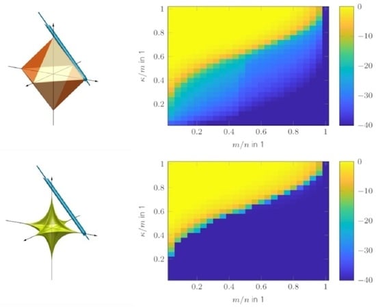
where determines how accurately the Kronecker function is approximated. An illustration of this approximation and other common approximations to the -quasi-norm are shown in Figure 6. As shown in [63], the series converges pointwise to as
An approximation to the -quasi-norm is therefore
where denotes a vector, which holds the magnitudes of the elements of s. The optimization Problem (1) may now be relaxed to
where the residual term was defined in (4) and is some constant noise energy. The constrained optimization Problem (41) can, for a fixed , be converted to an unconstrained optimization problem by use of regularization as
At this point, it should be noted that the Program (42) is not convex anymore but, rather, a sum of a concave and a convex function. As such, (42) does not possess a unique minimum, and it is possible to get stuck in local minimum. To circumvent this problem, the graduated non-convexity (GNC) approach is used. The idea of GNC is to start the Program (42) with a solution that is somewhat close to the true solution obtained from a convex algorithm, e.g., FISTA or TST. Then, (42) is minimized for a large enough such that the solution is closer to yet does not get stuck in a wrong local minimum. Subsequently, is reduced by a constant factor to further approximate the -quasi-norm, and (42) is minimized using the solution from the previous iteration. The procedure is conducted until a stop criterion is met.
For a fixed , the optimization Problem (42) can be solved by use of the iterative thresholding (IT) approach, similar to ISTA (22), by iteratively conducting
where is some step size and
is again an elementwise thresholding operator. Furthermore,
and denotes the upper branch of the multi-valued Lambert W function [54]. It should be noted that is a closed form solution of a subsequent minimization problem emerging from the IT approach. This closed form is possible only through the special choice of the -quasi-norm approximation (39), which leads to the possibility of applying the Lambert W function. For different choices, the subsequent minimization problem would require an additional minimization loop increasing the computational complexity. The regularization parameter is set to , where (33) is used for . Furthermore, the initial value is set to , where denotes the convex relaxed initial solution. More details regarding the CSCSA algorithm and the special selections of and are given in [54]. Finally, to further improve the convergence speed of the applied IT approach, a FISTA-like technique can be used as in [53], which does not increase the computational complexity but boosts the convergence rate from up to . Putting all the above steps together, the final CSCSA algorithm is listed in Algorithm 2. It consists of two loops, an inner and an outer one. In the outer loop is decreased gradually according to the GNC technique. The inner loop solves (42) by using a FISTA-like technique. The loops are aborted after a maximum number of iterations J and P or if the solution change, measured by the relative distance between consecutive solutions, drops below certain thresholds and . The threshold selections given in Algorithm 2 are taken from [63] and shown to work well in the following simulations.
| Algorithm 2 The CSCSA algorithm. |
| Input: A, y, λ, I, J Initialization:
|
Simulation results of a CSCSA update onto FISTA, SPGL1, and TST for random and DFT sensing operators are shown in Figure 7. For , (33) was used and the decreasing factor for was set to . As can be seen, CSCSA significantly improves upon the convex results shown in Figure 1. A comparison of the reconstruction performances is shown in Figure 8, in which the curves indicate the success rate with respect to the Monte Carlo runs. Success is defined as . In addition, the and success rate confidence intervals are indicated as shaded areas. The CSCSA refinement algorithm basically obtains similar reconstruction performance for every initialization algorithm as shown in Figure 8.
3. Affine Rank Minimization
In the following section, the TSVT and CSRA algorithms are introduced. Due to the structural similarity of CS and ARM algorithms, the TSVT and CSRA algorithms are also similar in structure to their CS counterparts from the former section. The TSVT algorithm obtains an initial low-rank convex solution, which is further refined by the CSRA algorithm. Their combination, likewise, yields all the desired properties of fast convergence and high reconstruction performance with no knowledge of generally unknown parameters, e.g., the true rank of etc.
3.1. Turbo Singular Value Thresholding
The TSVT algorithm is inspired by turbo affine rank minimization (TARM) presented in [57], which is solved for ARM problems applying the turbo principle. This principle allows for a drastic improvement in convergence speed for ROIL sensing operators to which random and DFT sensing operators belong. Within TARM, a HT operator is applied. Therefore, TARM was reworked here to use a ST operator. After finalizing TSVT, it came to the author’s attention, that a similar approach was formerly published in [56] called singular value thresholding-turbo-compressive sensing (SVT-Turbo-CS), conducting the same reconstruction as TSVT. The contributions of this work beyond SVT-Turbo-CS are twofold: (1) expansion into the complex case and (2) providing an equation to select the regularization parameter .
The TSVT algorithm attempts to find a solution to (2) by solving the convex relaxed regularized optimization Problem (20). This is achieved using the iterative procedure
where is some step size, i is the iteration index, and is the ST operator given by (25). The required parameters are chosen according to the turbo principle such that [57]
and that, furthermore, for a given , is minimized under (46) and (47). In the above equations, denotes the Frobenius product. Equation (46) ensures that the input and output error of the gradient update step are uncorrelated. Equally, (47) ensures a decorrelation of the input and output error of the denoising step. This strategy allows for an improved convergence rate compared to classical gradient approaches. In order to fulfill (46) and (47), the true solution is required to determine exact values for . Since is unknown, approximate formulations for were derived in [57] for the real valued case. In the general case these parameters are
For small scene sizes , it was found from simulations that the step size required for convergence has to be reduced to , which corresponds to the stable step size of the SVT algorithm. This phenomena was not discussed in [57,59], however, since the parameter Equations (48) to (50) are asymptotic approximations, and their validity requires the scene size to be sufficiently large. Nevertheless, TSVT still shows superior convergence speed even in the case of reduced step size. For the required divergence operator in (49), which is to be interpreted in the weak sense, i.e., it can fail to exist on negligible sets, a closed form solution exists [67] as
for or
for , when is simple, i.e., has no repeated singular values, and 0 otherwise. In (51) and (52), denotes the indicator function and
For more details on the derivation of , the reader is referred to [57]. The next question of course is how to choose the regularization parameter and thus which shrinkage should be applied. The usage of a ST operator causes the singular values of the optimal solution generated by the turbo framework (45) to possess an offset of a for every singular value compared with the true solution . Too much shrinkage results in a large bias, while too little results in a slow convergence rate. As such, an optimal constant does not exists, rather would need to be adjusted in every iteration. Unfortunately, to the best of the author’s knowledge, a closed form solution to determine such a is known to exist only for the signal model with the entries of being i. i. d. normally distributed [67]. However, this does not apply here, since the gradient update step as input to is not of such form. We therefore follow another approach and set the regularization parameter in a similar manner to (33) as
where is some constant, is the CDF of , and is some parameter. The additional factor of adjusts the threshold from (33) for singular values. For proofs of convergence, unique solutions, etc., of TARM and thus TSVT, the interested reader may have a look into [57].
Putting all the above steps together, the final TSVT algorithm is listed in Algorithm 3. It is aborted if an upper limit of iterations I is reached or if the relative change of the intermediate solutions
is below a predefined threshold . The threshold selection given in Algorithm 3 was evaluated numerically and proven to work well in every case.
In the following, simulation results are shown to illustrate the performance of TSVT. For all the following ARM algorithms presented, the SNR is defined as
and the recovery success is measured as SRE
The reconstruction performance is evaluated by use of phase transition plots, where for a given type of sensing operator (random or DFT) a number of low-rank matrices are to be reconstructed for different measurement ratios and degree of freedom ratios , where denotes the number of degrees of freedom in a rank- matrix. The low-rank matrices are set up by first determining and m from the given ratios. Here, it should be mentioned that since the rank has to be a whole number, it is not possible to clearly find a suitable integer for every possible . Instead, is determined by the closest integer to give the desired . Obviously, this only approximates the desired , where the approximation becomes better for larger dimensions . This, however, results in very high computation time. With this approach, the resulting may also result to zero, especially for small . In this case, no simulations were conducted, which are indicated by blank white entries in the following phase transition plots. A true low-rank matrix is set up as , where and are two orthonormalized matrices with elements drawn from an i. i. d. complex Gaussian distribution. Next, the sensing operators are set up, where for random sensing operators or for DFT operators is set up from m randomly selected rows of an DFT matrix following the identity . Finally, the elements of the noise vector n are drawn from an i. i. d. standard complex Gaussian distribution and scaled the given SNR according to (55). For every combination of measurement and rank ratio, 100 Monte Carlo runs were conducted and averaged to generate the phase transition plot. For the simulation results shown in the following , , , and is used.
| Algorithm 3 The TSVT algorithm. |
| Input: , y, λ, I Initialization:
|
As comparison benchmarks, the aforementioned simulations are also conducted for SVT, SVP, and TARM. The SVT algorithm is implemented according to [31], and its regularization parameter is set to (53). The SVP and TARM algorithms are likewise implemented according to [48,57] and equipped once with the true rank and once with . Both algorithms are aborted after a maximum number of iterations or if the relative improvement as defined in (54) is below a threshold similar to the TSVT algorithm.
The phase transition diagrams of the TSVT algorithm for random and DFT sensing operators are shown in Figure 9a,b. Its reconstruction performance is higher than SVT and SVP as shown in Figure 9c–f. The reconstruction performance of TARM in the case of the correctly chosen parameter is comparable to TSVT, as can be seen in Figure 9g,h. Interestingly, the DFT sensing operator reveals unfavorable properties for TARM in the upper right part of the phase transition plot shown in Figure 9h. This effect is also visible for TSVT as shown in Figure 9b, though less pronounced. The reason therefore is the rather structured nature of the DFT sensing operator, especially in the case of only a few randomly removed rows for a high measurement ratio . In [56], a similar effect is shown, but for CS and for correlated sparse signals. To fix this issue, the sensing operator was “improved” in [56] by adding more “randomness” to the DFT transformation by applying random signs to the columns of the glsdft matrix. In [57], such an augmented DFT matrix was also directly chosen. For radar, however, this approach is usually not possible, since the Fourier transform is inherently contained in the signal model. The reconstruction performance of TARM in the case of wrongly chosen parameter is shown in Figure 10. As can be seen, it depends heavily on R. The same holds for the convergence speed shown in Figure 11, which shows the intermediate SREs. The convergence speed of SVT is inferior and merely servers as a comparison benchmark. The convergence speed of SVP and TARM depend on the parameter R, where TARM outperforms SVP in any case. The convergence speed of TARM in the case of outperforms the TSVT algorithm, although it drops significantly in the case of . Compared with SVP, TSVT shows a faster or comparable convergence speed, depending on the sensing operator. For DFT sensing operators, the TSVT algorithm shows slower convergence speed than TARM and SVP. This is again due to the structured nature of the DFT sensing operator. While TARM and SVP can leverage the knowledge of to achieve fast convergence, TSVT requires more iterations. However, TARM and SVP are very sensitive to the selected value of R as illustrated by the dashed lines in Figure 11. A comparison of the computation time is shown in Figure 12 for a region where all algorithms perform equally well, except for SVT. The system specifications are the same as given in Section 2. The fastest algorithm is TARM provided is used. The second fastest is TSVT, followed by SVT and SVP. The computation time of TARM and SVP obviously increase in the case of , rendering TSVT a good choice in the case is unknown. Finally, the SRE for various SNRs is shown in Figure 13 for all tested algorithms. As can be seen, the best SREs offer TARM and SVP provided . Interestingly, the higher the available SNR, the worse is the achievable SRE in the case of . The TSVT algorithm follows the SRE of SVP and NIHT with an average loss of . The SVT algorithm provides a comparable SRE only for . In summary, TSVT is very easy to implement, shows a state-of-the-art convergence rate, has low computational complexity as there are closed form solutions available for all required parameters, and finally it does not require any unknown parameters, e.g., as the true rank of , in general. Hence, it is well suited for practical applications.
The reconstruction performance of the nuclear norm relaxed approaches can be further improved by use of smoothed rank techniques. A suitable and convenient version thereof is presented in the following section.
3.2. Complex Smoothed Rank Approximation
Although the performance of TSVT is already good, it can be improved in a similar manner as CSCSA does for TST results. The CSRA algorithm does so by enforcing a stricter rank measure than the nuclear norm used in (20). The CSRA algorithm is our extension based on the smoothed rank function (SRF) algorithm [61] and the SRA approach in [64]. CSRA is applicable to complex valued problems and in contrast to [64], has a closed form solution to a subsequent optimization problem, hence, reduced computational complexity. In the following, an overview of CSRA is given, while additional details can be found in the Appendix B.
To enforce a stricter rank measure, a different replacement for the rank function is proposed. The rank of , where , is defined as the number of nonzero elements in , where the vector holds the singular values of L. The rank of L can thus be defined as
where is the largest singular value of L and is the Kronecker delta function. Similar to CSCSA, (57) can be relaxed as
As can be seen, determines how close the rank function is approximated. Thus, an approximation to the rank function can be define as
The optimization problem (2) may now be relaxed to
where the data fidelity term was defined in (5). The constrained optimization problem (60) can be converted to an unconstrained one by use of regularization, which yields
where again is some regularization parameter. The minimization in (61) constitutes an alternative to the original problem given by (20). In this approach, is not concave nor convex (since is defined also for negative numbers due to evidential requirements) and not smooth, i.e., not differentiable at the origin. In order to avoid getting stuck in local minimum, the GNC approach is again applied similar to CSCSA. At first an initial solution is obtained from a convex optimization algorithm such as TSVT and is chosen big enough such that (62) does not get stuck in a local minimum. After convergence, is subsequently reduced until a stopping criterion is met. For a fixed , the optimization Problem (61) can be solved by the IT method, by iteratively solving
where is the SVD of the output of the gradient update step and is again a thresholding operator, which is given by (A25). In contrast to [64], a difference of convex (D.C.) optimization strategy to solve (61) is not needed; rather, the closed form solution is available. The regularization parameter is set to , where (53) is used for . This value was found from extensive numerical simulations to nicely balance the data fidelity error and the approximated rank function and perform well in any case. Furthermore, the initial value is set to , where denotes the convex relaxed initial solution. More details regarding the special selection of are given in the Appendix B. Finally, the convergence rate of the CSRA algorithm is accelerated using a FISTA-like technique [53]. Putting all the above steps together, the final CSRA algorithm is listed in Algorithm 4. The algorithm consists of two loops, an inner and an outer one. In the outer loop is decreased gradually according to the GNC technique. The inner loop solves (62) by using a FISTA-like technique. The loops are aborted after a maximum number of iterations J and P or if the solution changes, measured by the relative distance between consecutive solutions, drop below certain thresholds and . The threshold selections given in Algorithm 4 were found numerically as in [63] and were proven to work well in every case.
Simulation results for random and DFT sensing operators are shown in Figure 14. The decreasing factor for was set to . As can be seen, CSRA improves upon the convex results shown in Figure 9. If SVT was used as initialization algorithm for CSRA, the additional gain is dramatic for the random as well as the DFT sensing operator. If TSVT was used as an initialization algorithm, the improvements are not as high, because TSVT already achieves high reconstruction performance especially for random sensing operators. Nevertheless, especially for DFT sensing operators, CSRA helps to boost the reconstruction performance.
A comparison of the reconstruction performance of TSVT + CSRA to TARM is shown in Figure 15, in which the curves indicate a 50% success rate with respect to the Monte Carlo runs. Success is defined twofold as either for a strict success definition and for a less strict success definition. In addition, the and success rate confidence intervals are indicated as shaded areas. As can be seen, the combination of TSVT + CSRA follows and even outperforms TARM despite its non-awareness of the true rank .
| Algorithm 4 The CSRA algorithm. |
| Input: , y, λ, J, P Initialization:
|
In summary, CSRA in combination with TSVT is very easy to implement, shows a similar convergence rate and reconstruction performance as TARM equipped with the true rank of the unknown low-rank matrix in estimation, and has low computational complexity, as there are closed form solutions available for all required parameters and subsequent optimization problems. Finally, both do not generally require any unknown parameters. Hence, they are well suited for practical applications.
4. Compressed Robust Principle Component Analysis
Turbo Compressed Robust Principle Component Analysis
For TCRPCA, all of the aforementioned reconstruction algorithms for CS and ARM problems are combined together. Following the GNC approach described in Section 2.2, the corresponding relaxed convex Problem (21) is solved via a combination of TST and TSVT by iteratively updating
The required parameters , , and are determined as for the TST algorithm explained in Section 2.1 and , , , and as for the TSVT algorithm explained in Section 3.1. The regularization parameter is chosen as defined in (33). The combination of TST and TSVT is inspired by the turbo algorithms presented in [58,59]. In contrast to those works, only ST operators are used in the TCRPCA algorithm, whose parameters are not learned or determined via excessive grid search. Furthermore, in order to support the incoherence condition of the sparse and low-rank matrices and , the sparsity ratio operator and infinity norm operator may be applied [49]. The usage of prevents clustering of sparse entries and is defined element-wise as
where , denotes the - entry of S, the i- row, the j- column of S in Matlab notation, and the a- biggest entry in magnitude in . The usage of prevents spikiness in the low-rank reconstruction and is defined element-wise as
Unfortunately, the required parameters and are unknown in general. For , a reasonable guess is required and can be determined from
where is a parameter set manually usually [32,49]. Most parameters in (65) are unknown, since knowledge of the true low-rank matrix is required. As a rough estimate, we may use , , and . Certainly, this estimate is not justified to be anywhere close to an optimal value, but it was found from simulations that it is sufficient to apply and only for a limited number of iterations, e.g., the first 10 iterations. The intermediate results and then lie in a surrounding of a diffuse sparse and low-rank solution, and subsequent iterations do not need any further “guidance” by the projection operators. This also circumvents the problem of not knowing the optimal parameters and .
Once a suitable convex solution was obtained, a refinement is conducted by solving
where is the -approximation function (40) and is the rank approximation Function (59). Program (66) is solved via a combination of CSCSA and CSRA by iteratively updating
where is the thresholding operator as defined in CSCSA in Section 2.2 and is the thresholding operator as defined in CSRA in Section 3.2. The required parameters , , and are also the same as defined in CSCSA and CSRA.
Putting all the above steps together, the final TCRPCA algorithm is listed in Algorithm 5, which delivers a solution to program (21), and Algorithm 6 which solves for Program (66).
| Algorithm 5 Part 1 of TCRPCA algorithm delivering convex solution. |
| Input: , y, λs, λl, κs, φl, I Initialization:
|
In the following, simulation results are shown to illustrate the performance of TCRPCA for a DFT and a noiselet sensing operator instead of a random sensing operator for reasons of computational load. The sparse and low-rank matrices and are generated similar as for the aforementioned algorithms in Section 2 and Section 3, however, for a size of . The performance evaluation follows an approach similar as in [44]. The low-rank matrices are set up for fixed ranks and the phase transition plots are evaluated over the sparsity rate ; hence, the sparse matrices are accordingly set up. The resulting phase transition plots illustrated in Figure 16 indicate the success rate with respect to the Monte Carlo runs, where 20 runs are conducted. Success is defined as , where the SRE of the reconstructed low-rank matrices is used. These transition plots thus provide information of up to which sparsity rate or “corruption rate” the low-rank matrices can still be reconstructed.
| Algorithm 6 Part 2 of TCRPCA algorithm delivering refined solution. |
| Input: Initialization:
|
As comparison benchmarks, the aforementioned simulations are also conducted for SpaRCS, NFL, and TMP-CRPCA algorithm, which uses HT instead of ST denoisers. Additional comparisons of CRPCA algorithms are given in [68]. The SpaRCS algorithm is equipped with the true number of sparse entries and rank . Its implementation is taken from its official Github repository (https://github.com/image-science-lab/SpaRCS, accessed on 20 December 2022). The maximum number of iterations is set to , and for all remaining parameters the default setting is used. The NFL and TMP-CRPCA algorithms are implemented according to [44,59] and, likewise, equipped with the true number of sparse entries and rank . For the NFL algorithm, only the initial phase algorithm is used as the gradient descent phase algorithm merely serves as a final fast refinement step. For the initial phase algorithm, the maximum number of iterations of the Dykstra projection step are set to , and its corresponding infinity threshold value , as defined in (65), is chosen similar to the TCRPCA algorithm. The abortion criteria of NFL and TMP-CRPCA are also set as for the TCRPCA algorithm.
As can be seen in Figure 16a,b, the reconstruction performance of TCRPCA gracefully degrades with increasing rank . For the generation of these phase transition plots, no sparsity ratio operator and infinity norm operator are applied, since these have turned out to be unnecessary for , , and . The special cases of or are treated further below. The performance gain of the refinement step achieved by Part 2 of the TCRPCA algorithm appears moderate compared with the gains achieved in the pure CS and ARM applications. The reason therefore is that Part 1 of the TCRPCA algorithm shows a rather sharp transition in SRE, and thus Part 2 of TCRPCA lacks a sufficiently good initial solution to improve upon (not shown here). Nevertheless, the refinement step constitutes a computationally efficient and fast procedure offering increased reconstruction performance. In comparison, TMP-CRPCA and NFL shown in Figure 16c–f offer higher reconstruction performance for lower measurement rates , with NFL offering the highest. The results for SpaRCS illustrated in Figure 16g,h show a comparable performance in the case the rank of the low-rank matrix is as low as . Its performance, however, rapidly degrades with increasing rank . The reason therefore is that SpaRCS, in contrast to the remaining algorithms, lacks a sharp phase transition as illustrated in Figure 17. In this simulation, TMP-CRPCA, NFL, and SpaRCS are equipped with the true sparsity and rank parameters of the unknown matrices to reconstruct, namely and . In the case the parameters are set to and , all algorithms completely fail and, as such, are not shown here. A comparison of the convergence speed is shown in Figure 18, which shows the intermediate SREs. In this comparison, only Part 1 of the TCRPCA algorithm is shown. As can be seen, TMP-CRPCA, NFL, and SpaRCS show altogether a superior convergence rate compared with Part 1 of TCRPCA. This is in stark contrast to the pure CS and ARM counterparts shown in Section 2.1 and Section 3.1. Further evaluations revealed that Part 1 of TCRPCA requires of its iterations to correctly identify and , and the remaining iterations are used to minimize the reconstruction error. A comparison of the computation time is shown in Figure 19 for a region where all algorithms perform equally well. The system specifications are the same as given in Section 2. The overall fastest algorithm is TMP-CRPCA. In cases where the sensing operator can be implemented in an efficient manner, as is the case for the DFT sensing operator, the Part 1 TCRPCA algorithm offers the slowest computation time. In cases where the sensing operator is computationally more expansive to evaluate, Part 1 TCRPCA becomes more efficient and is faster than SpaRCS. The NFL algorithm is overall faster than in Part 1 TCRPCA. It should be noted that Part 1 TCRPCA can be aborted and Part 2 TCRPCA started sooner in order to reduce its overall computation time. This, however, is not done here for sake of clear evaluation. Finally, the SRE for various SNRs is shown in Figure 20 for all tested algorithms. For Part 1 of TCRPCA, the performance is shown with and without the spikiness operator defined in (65) for . As can be seen, for , the spikiness operator is required to support the reconstruction, especially for higher sparsity ratios . In the case of higher SNRs, no supporting operator is required anymore; in fact, it is obstructive at high SNR. For these simulations, no sparsity ratio operator is required. The best SRE offer TMP-CRPCA and NFL provided and .
For CRPCA, and represent special cases. In order to allow for successful reconstructions in the case of , it is found from simulations that the sparsity ratio operator is required for all iterations with a setting of to allow for a successful identification of . Likewise, the infinity norm operator with a setting of is found to be required for all iterations to successfully identify the special case of . The use of the sparsity ratio and infinity norm operators incur restrictions regarding the possible reconstruction performance of the TCRPCA algorithm. Obviously, the use of with prohibits successful reconstructions in the case of . In a similar manner, the use of with prohibits successful reconstructions in the case . How to treat the special cases of either or in a satisfactory manner, i.e., how to relax and conveniently, is an open question and subject to further investigation. The obvious approach of conducting a CS, an ARM, and an CRPCA reconstruction separately and comparing the resulting residual errors to determine if either or does not work. Particularly in the case of low , the CRPCA approach always yields the lowest residual error regardless if the scene is strictly sparse or low-rank due to its larger degree of freedom.
In summary, TCRPCA offers comparable reconstruction performance to its greedy and HT counterparts despite its unawareness of the true sparsity and rank values. It is very easy to implement and has low computational complexity, as there are closed form solutions available for all required parameters and subsequent optimization problems. In the case of and , no generally unknown parameters are required for successful reconstruction. Hence, TCRPCA is well suited for practical applications. In the special cases or , TCRPCA is capable of a successful reconstruction if or , respectively.
5. Conclusions
In this paper, fast, efficient, and viable CS, ARM, and CRPCA algorithms suitable for radar signal processing are proposed. They are designed such that no parameters unknown in practice, e.g., the number of sparse entries or the rank of the unknown low-rank matrix, are required. The only parameter that is needed to be known is the noise power, which in the field of radar signal processing is usually available. For all remaining parameters, either suitable heuristic formulas or closed form solutions are given. The general reconstruction scheme comprises two steps: First, a convex solution is calculated for which the turbo-message-passing framework is utilized. This initial solution is in a second step refined by use of smoothed -refinements. The proposed algorithms for CS are termed TST and CSCSA, for ARM problems TSVT and CSRA, and TCRPCA for the combined CS and ARM problems. All algorithms show state-of-the-art reconstruction performance and are of high computational efficiency, as closed form solutions are available for subsequent optimization tasks.
Funding
This research was funded by Hensoldt Sensor GmbH.
Data Availability Statement
Not applicable.
Conflicts of Interest
The author declares no conflict of interest. In addition, the funders had no role in the writing of the manuscript.
Appendix A. Divergence of the Complex Soft-Thresholding Operator
In this section, the weak divergence of the complex soft thresholding operator is derived in closed form, which is defined as [69]
where , , and
is the complex sign function. A useful alternative formulation of the second term in (A1) is
Furthermore, for some matrix , the complex soft thresholding operator is defined as an element-wise operation as
with and . Finally, the definition of the divergence for a scalar complex function is
and for a multidimensional function [70]
The mapping f or may not be differentiable everywhere. Fortunately, in the case of weak divergence, only weak differentiability is required. For such, sets of Lebesgue measure zero can be discarded [67]. Combining (A4) and (A5) yields the desired divergence
Using (A3), the required derivative is
After a few steps, the derivative in results in
where the discontinuity at can be discarded since for . The derivative in yields
Appendix B. Complex Smoothed Rank Approximation
In this section, a minimization procedure to acquire a solution to the regularized smoothed rank Problem (61)
is derived. The smoothed rank function was defined in (59) as
where is given by (58). In program (A10), is convex and differentiable with Lipschitz continuous gradient whereas is neither concave nor convex (since is also defined for negative numbers due to evidential requirements) and not differentiable at the origin. Nevertheless, the IT method can be utilized to conduct the desired minimization: For a fixed , a solution to program (A10) can be obtained by iteratively solving
until convergence, where is some step size and
is the result of a gradient update step [63]. In order to minimize (A12), the following two theorems are useful.
Theorem A1.
The function is unitarily invariant if provided is absolutely symmetric, i.e., is invariant under arbitrary permutations and sign changes of the elements of [60].
This property applies to the rank approximation function defined in (A11).
Theorem A2.
For unitarily invariant functions the optimal solution to the problem
is
where is the SVD decomposition of and is obtained by solving the separable minimization problem
where [60].
It should be noted that Theorem A2 also works if would not be a unitarily invariant function, provided , where , which is inherently fulfilled since is a real positive diagonal matrix. By use of Theorem A2, a solution to (A12) is obtained as
where
is the SVD of , , and
where . The objective function (A16) is the sum of a concave and convex function (since ). To the contrary of [64], we do not solve (A16) by applying a D.C. optimization strategy which would require multiple iterations. An alternative approach, first shown in [63], is to utilize the Lambert W function
which allows for a closed form solution of (A16). We start by noticing that the minimization in (A16) is separable and as such can be conducted element wise as
Defining the argument of (A18) as
taking its derivative with respect to and setting it to zero yields after short manipulation
where we used the fact that . To apply the Lambert W function we modify (A20) to
Applying the Lambert W function on both sides of (A21) gives two solutions
where
and denotes the upper branch and the lower branch of the multi-valued Lambert W function. As shown in [63], it can be proven that from (A23) cannot be the minimizer of (A18). The rest of the derivation, which establishes conditions under which is the true minimizer of (A18), is left to look up in [63]. In consequence, the solution to (A18) is the shrinkage operator
where is defined in (A22) and in (A19). The solution to (A12) is therefore
where is the vector operator version of (A25), , is (A13), and and are defined in (A15).
The structure of the CSRA algorithm is similar to the SCSA algorithm presented in [63], which was designed for real valued CS problems. Hence, the convergence proof given in [63] can readily be adapted to the CSRA algorithm and is therefore not recapitulated here. Only the following theorem stating the convergence shall be given, in which h denotes the data fidelity term defined in (5).
Theorem A3.
The proof of Theorem A3 is equivalent to the proof given in [63] when replacing all norms and inner products with the Frobenius norm and Frobenius product. The Lipschitz constant of is given by the squared operator norm . However, a formal proof of the existence of , which would need to fulfill
is open. Nevertheless, a step size of resulted in converging behavior in all conducted simulations. An alternative proof of convergence is given in [64], however for a decreasing step size.
Finally, a few words on the initialization of are in order. Let be the unique solution to
which is the equivalent nuclear norm minimization (NNM) noiseless optimization problem to (17). In [62] it was shown, that for , the following statement holds
provided that (A26) has a unique solution. Therefore, (60), for , can be optimized by solving (17) for which SVT or TSVT may be used. According to [62], is a reasonable choice such that (A27) approximately holds. For CSRA, was found to work well in every case.
References
- Ender, J.H. On compressive sensing applied to radar. Signal Process. 2010, 90, 1402–1414. [Google Scholar] [CrossRef]
- Weng, Z.; Wang, X. Low-rank matrix completion for array signal processing. In Proceedings of the 2012 IEEE International Conference on Acoustics, Speech and Signal Processing (ICASSP), Kyoto, Japan, 25–30 March 2012; pp. 2697–2700. [Google Scholar] [CrossRef]
- Ender, J. A brief review of compressive sensing applied to radar. In Proceedings of the 2013 14th International Radar Symposium (IRS), Dresden, Germany, 19–21 June 2013; Volume 1, pp. 3–16. [Google Scholar]
- de Lamare, R.C. Low-Rank Signal Processing: Design, Algorithms for Dimensionality Reduction and Applications. arXiv 2015, arXiv:1508.00636. [Google Scholar] [CrossRef]
- Sun, S.; Mishra, K.V.; Petropulu, A.P. Target Estimation by Exploiting Low Rank Structure in Widely Separated MIMO Radar. In Proceedings of the 2019 IEEE Radar Conference (RadarConf), Boston, MA, USA, 22–26 April 2019; pp. 1–6. [Google Scholar] [CrossRef]
- Xiang, Y.; Xi, F.; Chen, S. LiQuiD-MIMO Radar: Distributed MIMO Radar with Low-Bit Quantization. arXiv 2023, arXiv:eess.SP/2302.08271. [Google Scholar]
- Rangaswamy, M.; Lin, F. Radar applications of low rank signal processing methods. In Proceedings of the Thirty-Sixth Southeastern Symposium on System Theory, Atlanta, GA, USA, 16 March 2004; pp. 107–111. [Google Scholar] [CrossRef]
- Prünte, L. GMTI on short sequences of pulses with compressed sensing. In Proceedings of the 2015 3rd International Workshop on Compressed Sensing Theory and its Applications to Radar, Sonar and Remote Sensing (CoSeRa), Pisa, Italy, 17–19 June 2015; pp. 66–70. [Google Scholar] [CrossRef]
- Sen, S. Low-Rank Matrix Decomposition and Spatio-Temporal Sparse Recovery for STAP Radar. IEEE J. Sel. Top. Signal Process. 2015, 9, 1510–1523. [Google Scholar] [CrossRef]
- Prünte, L. Compressed sensing for the detection of moving targets from short sequences of pulses: Special section “sparse reconstruction in remote sensing”. In Proceedings of the 2016 4th International Workshop on Compressed Sensing Theory and its Applications to Radar, Sonar and Remote Sensing (CoSeRa), Aachen, Germany, 19–22 September 2016; pp. 85–89. [Google Scholar] [CrossRef]
- Prünte, L. Detection of Moving Targets Using Off-Grid Compressed Sensing. In Proceedings of the 2018 19th International Radar Symposium (IRS), Bonn, Germany, 20–22 June 2018; pp. 1–10. [Google Scholar] [CrossRef]
- Dao, M.; Nguyen, L.; Tran, T.D. Temporal rate up-conversion of synthetic aperture radar via low-rank matrix recovery. In Proceedings of the 2013 IEEE International Conference on Image Processing, Melbourne, VIC, Australia, 15–18 September 2013; pp. 2358–2362. [Google Scholar] [CrossRef]
- Cerutti-Maori, D.; Prünte, L.; Sikaneta, I.; Ender, J. High-resolution wide-swath SAR processing with compressed sensing. In Proceedings of the 2014 IEEE Geoscience and Remote Sensing Symposium, Quebec City, QC, Canada, 13–18 July 2014; pp. 3830–3833. [Google Scholar] [CrossRef]
- Mason, E.; Son, I.-Y.; Yazici, B. Passive synthetic aperture radar imaging based on low-rank matrix recovery. In Proceedings of the 2015 IEEE Radar Conference (RadarCon), Arlington, VA, USA, 10–15 May 2015; pp. 1559–1563. [Google Scholar]
- Kang, J.; Wang, Y.; Schmitt, M.; Zhu, X.X. Object-Based Multipass InSAR via Robust Low-Rank Tensor Decomposition. IEEE Trans. Geosci. Remote Sens. 2018, 56, 3062–3077. [Google Scholar] [CrossRef] [Green Version]
- Hamad, A.; Ender, J. Three Dimensional ISAR Autofocus based on Sparsity Driven Motion Estimation. In Proceedings of the 2020 21st International Radar Symposium (IRS), Warsaw, Poland, 5–8 October 2020; pp. 51–56. [Google Scholar] [CrossRef]
- Qiu, W.; Zhou, J.; Fu, Q. Jointly Using Low-Rank and Sparsity Priors for Sparse Inverse Synthetic Aperture Radar Imaging. IEEE Trans. Image Process. 2020, 29, 100–115. [Google Scholar] [CrossRef]
- Wagner, S.; Ender, J. Scattering Identification in ISAR Images via Sparse Decomposition. In Proceedings of the 2022 IEEE Radar Conference (RadarConf22), New York, NY, USA, 21–25 March 2022; pp. 1–6. [Google Scholar] [CrossRef]
- Tang, V.H.; Bouzerdoum, A.; Phung, S.L.; Tivive, F.H.C. Radar imaging of stationary indoor targets using joint low-rank and sparsity constraints. In Proceedings of the 2016 IEEE International Conference on Acoustics, Speech and Signal Processing (ICASSP), Shanghai, China, 20–25 March 2016; pp. 1412–1416. [Google Scholar] [CrossRef] [Green Version]
- Sun, Y.; Breloy, A.; Babu, P.; Palomar, D.P.; Pascal, F.; Ginolhac, G. Low-Complexity Algorithms for Low Rank Clutter Parameters Estimation in Radar Systems. IEEE Trans. Signal Process. 2016, 64, 1986–1998. [Google Scholar] [CrossRef]
- Wang, J.; Ding, M.; Yarovoy, A. Interference Mitigation for FMCW Radar with Sparse and Low-Rank Hankel Matrix Decomposition. IEEE Trans. Signal Process. 2022, 70, 822–834. [Google Scholar] [CrossRef]
- Brehier, H.; Breloy, A.; Ren, C.; Hinostroza, I.; Ginolhac, G. Robust PCA for Through-the-Wall Radar Imaging. In Proceedings of the 2022 30th European Signal Processing Conference (EUSIPCO), Belgrade, Serbia, 29 August–2 September 2022; pp. 2246–2250. [Google Scholar] [CrossRef]
- Yang, D.; Yang, X.; Liao, G.; Zhu, S. Strong Clutter Suppression via RPCA in Multichannel SAR/GMTI System. IEEE Geosci. Remote Sens. Lett. 2015, 12, 2237–2241. [Google Scholar] [CrossRef]
- Guo, Y.; Liao, G.; Li, J.; Chen, X. A Novel Moving Target Detection Method Based on RPCA for SAR Systems. IEEE Trans. Geosci. Remote Sens. 2020, 58, 6677–6690. [Google Scholar] [CrossRef]
- A Clutter Suppression Method Based on NSS-RPCA in Heterogeneous Environments for SAR-GMTI. IEEE Trans. Geosci. Remote Sens. 2020, 58, 5880–5891. [CrossRef]
- Yang, J.; Jin, T.; Xiao, C.; Huang, X. Compressed Sensing Radar Imaging: Fundamentals, Challenges, and Advances. Sensors 2019, 19, 3100. [Google Scholar] [CrossRef] [PubMed] [Green Version]
- Zuo, L.; Wang, J.; Zhao, T.; Cheng, Z. A Joint Low-Rank and Sparse Method for Reference Signal Purification in DTMB-Based Passive Bistatic Radar. Sensors 2021, 21, 3607. [Google Scholar] [CrossRef] [PubMed]
- De Maio, A.; Eldar, Y.; Haimovich, A. Compressed Sensing in Radar Signal Processing; Cambridge University Press: Cambridge, UK, 2019. [Google Scholar]
- Amin, M. Compressive Sensing for Urban Radar; CRC Press: Boca Raton, FL, USA, 2017. [Google Scholar]
- Manchanda, R.; Sharma, K. A Review of Reconstruction Algorithms in Compressive Sensing. In Proceedings of the 2020 International Conference on Advances in Computing, Communication Materials (ICACCM), Dehradun, India, 21–22 August 2020; pp. 322–325. [Google Scholar] [CrossRef]
- Cai, J.F.; Candès, E.J.; Shen, Z. A Singular Value Thresholding Algorithm for Matrix Completion. arXiv 2008, arXiv:math.OC/0810.3286. [Google Scholar] [CrossRef]
- Candès, E.J.; Li, X.; Ma, Y.; Wright, J. Robust Principal Component Analysis? CoRR 2009. abs/0912.3599. [Google Scholar] [CrossRef]
- Eldar, Y.; Kutyniok, G. Compressed Sensing: Theory and Applications; Cambridge University Press: Cambridge, UK, 2012. [Google Scholar]
- Pilastri, A.; Tavares, J. Reconstruction Algorithms in Compressive Sensing: An Overview. In Proceedings of the FAUP-11th Edition of the Doctoral Symposium in Informatics Engineering, Porto, Portugal, 3 February 2016. [Google Scholar]
- Park, D.; Kyrillidis, A.; Caramanis, C.; Sanghavi, S. Finding Low-Rank Solutions via Non-Convex Matrix Factorization, Efficiently and Provably. arXiv 2016, arXiv:1606.03168. [Google Scholar] [CrossRef]
- Chandrasekaran, V.; Sanghavi, S.; Parrilo, P.A.; Willsky, A.S. Rank-Sparsity Incoherence for Matrix Decomposition. SIAM J. Optim. 2011, 21, 572–596. [Google Scholar] [CrossRef]
- Tropp, J.A.; Gilbert, A.C. Signal recovery from random measurements via orthogonal matching pursuit. IEEE Trans. Inf. Theory 2007, 53, 4655–4666. [Google Scholar] [CrossRef] [Green Version]
- Donoho, D.L.; Tsaig, Y.; Drori, I.; Starck, J.L. Sparse solution of underdetermined systems of linear equations by stagewise orthogonal matching pursuit. IEEE Trans. Inf. Theory 2012, 58, 1094–1121. [Google Scholar] [CrossRef]
- Needell, D.; Vershynin, R. Signal recovery from incomplete and inaccurate measurements via regularized orthogonal matching pursuit. IEEE J. Sel. Top. Signal Process. 2010, 4, 310–316. [Google Scholar] [CrossRef] [Green Version]
- Needell, D.; Tropp, J.A. CoSaMP: Iterative signal recovery from incomplete and inaccurate samples. Appl. Comput. Harmon. Anal. 2009, 26, 301–321. [Google Scholar] [CrossRef] [Green Version]
- Dai, W.; Milenkovic, O. Subspace pursuit for compressive sensing signal reconstruction. IEEE Trans. Inf. Theory 2009, 55, 2230–2249. [Google Scholar] [CrossRef] [Green Version]
- Boche, H.; Calderbank, R.; Kutyniok, G.; Vybiral, J. A Survey of Compressed Sensing; Springer: Berlin/Heidelberg, Germany, 2014. [Google Scholar] [CrossRef]
- Lee, K.; Bresler, Y. ADMiRA: Atomic Decomposition for Minimum Rank Approximation. IEEE Trans. Inf. Theory 2010, 56, 4402–4416. [Google Scholar] [CrossRef] [Green Version]
- Waters, A.; Sankaranarayanan, A.; Baraniuk, R. SpaRCS: Recovering low-rank and sparse matrices from compressive measurements. In Proceedings of the Advances in Neural Information Processing Systems; Shawe-Taylor, J., Zemel, R., Bartlett, P., Pereira, F., Weinberger, K., Eds.; Curran Associates, Inc.: Red Hook, NY, USA, 2011; Volume 24. [Google Scholar]
- Xiang, J.; Yue, H.; Xiangjun, Y.; Guoqing, R. A Reweighted Symmetric Smoothed Function Approximating L0-Norm Regularized Sparse Reconstruction Method. Symmetry 2018, 10, 583. [Google Scholar] [CrossRef] [Green Version]
- Xiang, J.; Yue, H.; Xiangjun, Y.; Wang, L. A New Smoothed L0 Regularization Approach for Sparse Signal Recovery. Math. Probl. Eng. 2019, 2019, 1978154. [Google Scholar] [CrossRef] [Green Version]
- Blumensath, T.; Davies, M.E. Normalized Iterative Hard Thresholding: Guaranteed Stability and Performance. IEEE J. Sel. Top. Signal Process. 2010, 4, 298–309. [Google Scholar] [CrossRef] [Green Version]
- Meka, R.; Jain, P.; Dhillon, I.S. Guaranteed Rank Minimization via Singular Value Projection. arXiv 2009, arXiv:cs.LG/0909.5457. [Google Scholar]
- Zhang, X.; Wang, L.; Gu, Q. A Unified Framework for Low-Rank plus Sparse Matrix Recovery. arXiv 2017, arXiv:1702.06525. [Google Scholar] [CrossRef]
- Blanchard, J.D.; Tanner, J. Performance comparisons of greedy algorithms in compressed sensing. Numer. Linear Algebra Appl. 2015, 22, 254–282. [Google Scholar] [CrossRef] [Green Version]
- Mansour, H. Beyond ℓ1-norm minimization for sparse signal recovery. In Proceedings of the 2012 IEEE Statistical Signal Processing Workshop (SSP), Ann Arbor, MI, USA, 5–8 August 2012; pp. 337–340. [Google Scholar] [CrossRef]
- Aravkin, A.; Becker, S.; Cevher, V.; Olsen, P. A variational approach to stable principal component pursuit. arXiv 2014, arXiv:1406.1089. [Google Scholar] [CrossRef]
- Beck, A.; Teboulle, M. A fast iterative shrinkage-thresholding algorithm for linear inverse problems. SIAM J. Imaging Sci. 2009, 2, 183–202. [Google Scholar] [CrossRef] [Green Version]
- Panhuber, R.; Prünte, L. Complex Successive Concave Sparsity Approximation. In Proceedings of the 2020 21st International Radar Symposium (IRS), Warsaw, Poland, 5–8 October 2020; pp. 67–72. [Google Scholar] [CrossRef]
- Ma, J.; Yuan, X.; Ping, L. Turbo Compressed Sensing with Partial DFT Sensing Matrix. IEEE Signal Process. Lett. 2015, 22, 158–161. [Google Scholar] [CrossRef] [Green Version]
- Xue, Z.; Ma, J.; Yuan, X. Denoising-Based Turbo Compressed Sensing. IEEE Access 2017, 5, 7193–7204. [Google Scholar] [CrossRef]
- Xue, Z.; Yuan, X.; Ma, J.; Ma, Y. TARM: A Turbo-Type Algorithm for Affine Rank Minimization. IEEE Trans. Signal Process. 2019, 67, 5730–5745. [Google Scholar] [CrossRef] [Green Version]
- Xue, Z.; Yuan, X.; Yang, Y. Turbo-Type Message Passing Algorithms for Compressed Robust Principal Component Analysis. IEEE J. Sel. Top. Signal Process. 2018, 12, 1182–1196. [Google Scholar] [CrossRef]
- He, X.; Xue, Z.; Yuan, X. Learned Turbo Message Passing for Affine Rank Minimization and Compressed Robust Principal Component Analysis. IEEE Access 2019, 7, 140606–140617. [Google Scholar] [CrossRef]
- Kang, Z.; Peng, C.; Cheng, J.; Cheng, Q. LogDet Rank Minimization with Application to Subspace Clustering. Comput. Intell. Neurosci. 2015, 2015, 824289. [Google Scholar] [CrossRef] [Green Version]
- Malek-Mohammadi, M.; Babaie-Zadeh, M.; Amini, A.; Jutten, C. Recovery of Low-Rank Matrices Under Affine Constraints via a Smoothed Rank Function. IEEE Trans. Signal Process. 2014, 62, 981–992. [Google Scholar] [CrossRef] [Green Version]
- Malek-Mohammadi, M.; Babaie-Zadeh, M.; Skoglund, M. Iterative Concave Rank Approximation for Recovering Low-Rank Matrices. IEEE Trans. Signal Process. 2014, 62, 5213–5226. [Google Scholar] [CrossRef] [Green Version]
- Malek-Mohammadi, M.; Koochakzadeh, A.; Babaie-Zadeh, M.; Jansson, M.; Rojas, C. Successive Concave Sparsity Approximation for Compressed Sensing. IEEE Trans. Signal Process. 2016, 64, 5657–5671. [Google Scholar] [CrossRef] [Green Version]
- Ye, H.; Li, H.; Yang, B.; Cao, F.; Tang, Y. A Novel Rank Approximation Method for Mixture Noise Removal of Hyperspectral Images. IEEE Trans. Geosci. Remote Sens. 2019, 57, 4457–4469. [Google Scholar] [CrossRef]
- Bickel, P.J.; Ritov, Y.; Tsybakov, A.B. Simultaneous analysis of Lasso and Dantzig selector. arXiv 2008, arXiv:0801.1095. [Google Scholar] [CrossRef]
- Donoho, D.; Tanner, J. Observed universality of phase transitions in high-dimensional geometry, with implications for modern data analysis and signal processing. Philos. Trans. R. Soc. Math. Phys. Eng. Sci. 2009, 367, 4273–4293. [Google Scholar] [CrossRef] [PubMed]
- Candès, E.J.; Sing-Long, C.A.; Trzasko, J.D. Unbiased Risk Estimates for Singular Value Thresholding and Spectral Estimators. IEEE Trans. Signal Process. 2013, 61, 4643–4657. [Google Scholar] [CrossRef] [Green Version]
- Bouwmans, T.; Sobral, A.; Javed, S.; Jung, S.K.; Zahzah, E.H. Decomposition into low-rank plus additive matrices for background/foreground separation: A review for a comparative evaluation with a large-scale dataset. Comput. Sci. Rev. 2017, 23, 1–71. [Google Scholar] [CrossRef] [Green Version]
- Foucart, S.; Rauhut, H. A Mathematical Introduction to Compressive Sensing; Springer: Berlin/Heidelberg, Germany, 2013. [Google Scholar] [CrossRef]
- Zill, D.; Wright, W. Differential Equations with Boundary-Value Problems; Cengage Learning: Boston, MA, USA, 2012. [Google Scholar]
Figure 1.
Phase transition of CS algorithms in SRE in dB.

Figure 2.
Phase transition plot for NIHT in the case of wrongly chosen parameter .

Figure 3.
Comparison of convergence speed for = 0.25 and . The solid line shows NIHT for and the dashed line . (a) Random sensing operators . (b) DFT sensing operators with random rows.
Figure 3.
Comparison of convergence speed for = 0.25 and . The solid line shows NIHT for and the dashed line . (a) Random sensing operators . (b) DFT sensing operators with random rows.

Figure 4.
Comparison of computation time . The solid line shows NIHT for and the dashed line . (a) Random sensing operators . (b) DFT sensing operators with random rows.
Figure 4.
Comparison of computation time . The solid line shows NIHT for and the dashed line . (a) Random sensing operators . (b) DFT sensing operators with random rows.

Figure 5.
Comparison of SRE vs. SNR for . The solid line for NIHT shows and the dashed line . (a) Random sensing operators for . (b) DFT sensing operator for . (c) Random sensing operators for . (d) DFT sensing operator for . (e) Random sensing operators for . (f) DFT sensing operator for . (g) Random sensing operators for . (h) DFT sensing operator for .

Figure 6.
Common approximations to the -quasi-norm.

Figure 7.
Phase transition of refined CS algorithms in SRE in dB.


Figure 8.
Comparison of reconstruction performances for CSCSA update. Reconstruction success is defined as .
Figure 8.
Comparison of reconstruction performances for CSCSA update. Reconstruction success is defined as .

Figure 9.
Phase transition of ARM algorithms in SRE in dB.


Figure 10.
Phase transition plot for TARM in the case of wrongly chosen parameter .

Figure 11.
Comparison of convergence speed for and . The solid lines show SVP and TARM for and the dashed lines for . (a) Random sensing operators . (b) DFT sensing operators with random rows.
Figure 11.
Comparison of convergence speed for and . The solid lines show SVP and TARM for and the dashed lines for . (a) Random sensing operators . (b) DFT sensing operators with random rows.

Figure 12.
Comparison of computation time for in an interval where all algorithms perform equally well. The solid lines show SVP and TARM for and the dashed lines for . (a) Random sensing operators . (b) DFT sensing operators with random rows.
Figure 12.
Comparison of computation time for in an interval where all algorithms perform equally well. The solid lines show SVP and TARM for and the dashed lines for . (a) Random sensing operators . (b) DFT sensing operators with random rows.

Figure 13.
Comparison of SRE vs. SNR for . The solid line for SVP and TARM show and the dashed line . (a) Random sensing operators for . (b) DFT sensing operator for . (c) Random sensing operators for . (d) DFT sensing operator for . (e) Random sensing operators for . (f) DFT sensing operator for . (g) Random sensing operators for . (h) DFT sensing operator for .


Figure 14.
Phase transition of refined ARM algorithms in SRE in dB.

Figure 15.
Comparison of reconstruction performances of TSVT + CSRA to TARM. The solid lines show the 50% success rate for a strict reconstruction success, defined as , and the dashed lines the success rate for a less strict success definition, i.e., .
Figure 15.
Comparison of reconstruction performances of TSVT + CSRA to TARM. The solid lines show the 50% success rate for a strict reconstruction success, defined as , and the dashed lines the success rate for a less strict success definition, i.e., .

Figure 16.
Comparison of reconstruction performance. Dashed lines illustrate results of Part 1 of the TCRPCA algorithm given by Algorithm 5 and solid lines the refined results achieved by Part 2 the TCRPCA algorithm given by Algorithm 6. (a) TCRPCA for noiselet operator. (b) TCRPCA for DFT operator. (c) turbo message passing for CRPCA (TMP-CRPCA) for noiselet operator with and . (d) TMP-CRPCA for DFT operator with and . (e) NFL for noiselet operator with and . (f) NFL for DFT operator with and . (g) SpaRCS for noiselet operator with and . (h) SpaRCS for DFT operator with and .


Figure 17.
In detail reconstruction performance comparison for a DFT sensing operator and . The red line indicates the success boundary or the phase transitions shown in Figure 16.
Figure 17.
In detail reconstruction performance comparison for a DFT sensing operator and . The red line indicates the success boundary or the phase transitions shown in Figure 16.

Figure 18.
Comparison of convergence speed for , and . The solid lines show NFL, SpaRCS, and TMP-CRPCA for and and the dashed lines for and .
Figure 18.
Comparison of convergence speed for , and . The solid lines show NFL, SpaRCS, and TMP-CRPCA for and and the dashed lines for and .

Figure 19.
Comparison of computation time for and , i.e., in an interval where all algorithms perform equally well. For NFL, SpaRCS, and TMP-CRPCA, the results are shown for and only. For , TMP-CRPCA did not converge and is thus not shown here. (a) Noislet sensing operators. (b) DFT sensing operators with random rows.

Figure 20.
Comparison of the low-rank SRE vs. SNR for . The solid line for TCRPCA shows the performance without and the dashed line with the spikiness operator defined in (64), respectively.
Figure 20.
Comparison of the low-rank SRE vs. SNR for . The solid line for TCRPCA shows the performance without and the dashed line with the spikiness operator defined in (64), respectively.


Disclaimer/Publisher’s Note: The statements, opinions and data contained in all publications are solely those of the individual author(s) and contributor(s) and not of MDPI and/or the editor(s). MDPI and/or the editor(s) disclaim responsibility for any injury to people or property resulting from any ideas, methods, instructions or products referred to in the content. |
© 2023 by the author. Licensee MDPI, Basel, Switzerland. This article is an open access article distributed under the terms and conditions of the Creative Commons Attribution (CC BY) license (https://creativecommons.org/licenses/by/4.0/).
Share and Cite
MDPI and ACS Style
Panhuber, R. Fast, Efficient, and Viable Compressed Sensing, Low-Rank, and Robust Principle Component Analysis Algorithms for Radar Signal Processing. Remote Sens. 2023, 15, 2216. https://doi.org/10.3390/rs15082216
AMA Style
Panhuber R. Fast, Efficient, and Viable Compressed Sensing, Low-Rank, and Robust Principle Component Analysis Algorithms for Radar Signal Processing. Remote Sensing. 2023; 15(8):2216. https://doi.org/10.3390/rs15082216
Chicago/Turabian StylePanhuber, Reinhard. 2023. "Fast, Efficient, and Viable Compressed Sensing, Low-Rank, and Robust Principle Component Analysis Algorithms for Radar Signal Processing" Remote Sensing 15, no. 8: 2216. https://doi.org/10.3390/rs15082216
Note that from the first issue of 2016, this journal uses article numbers instead of page numbers. See further details here.