
An Advanced Spatiotemporal Fusion Model for Suspended Particulate Matter Monitoring in an Intermontane Lake
 ,
,  , ,
, ,
Abstract
:1. Introduction
2. Materials
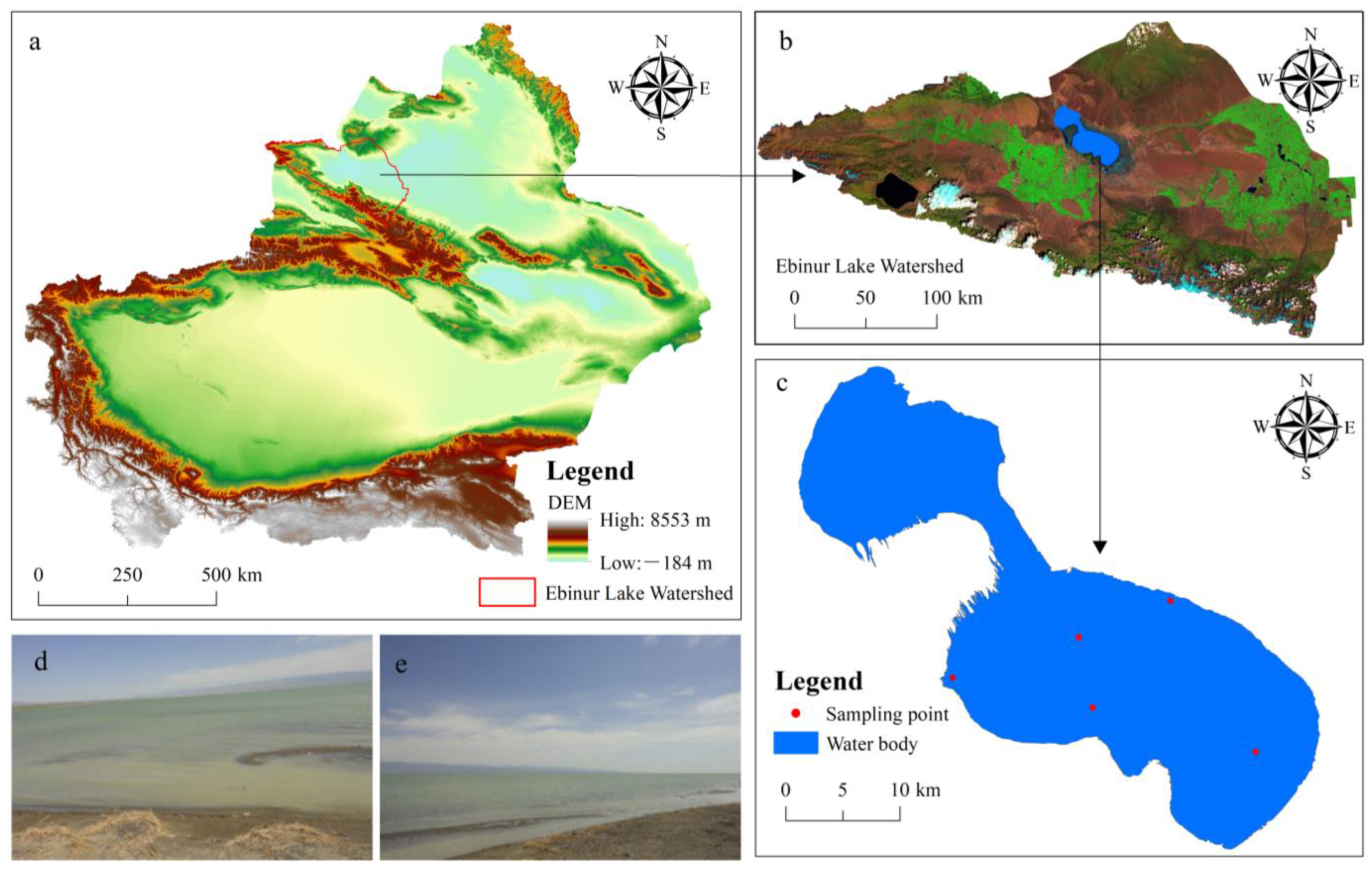
2.1. Study Area
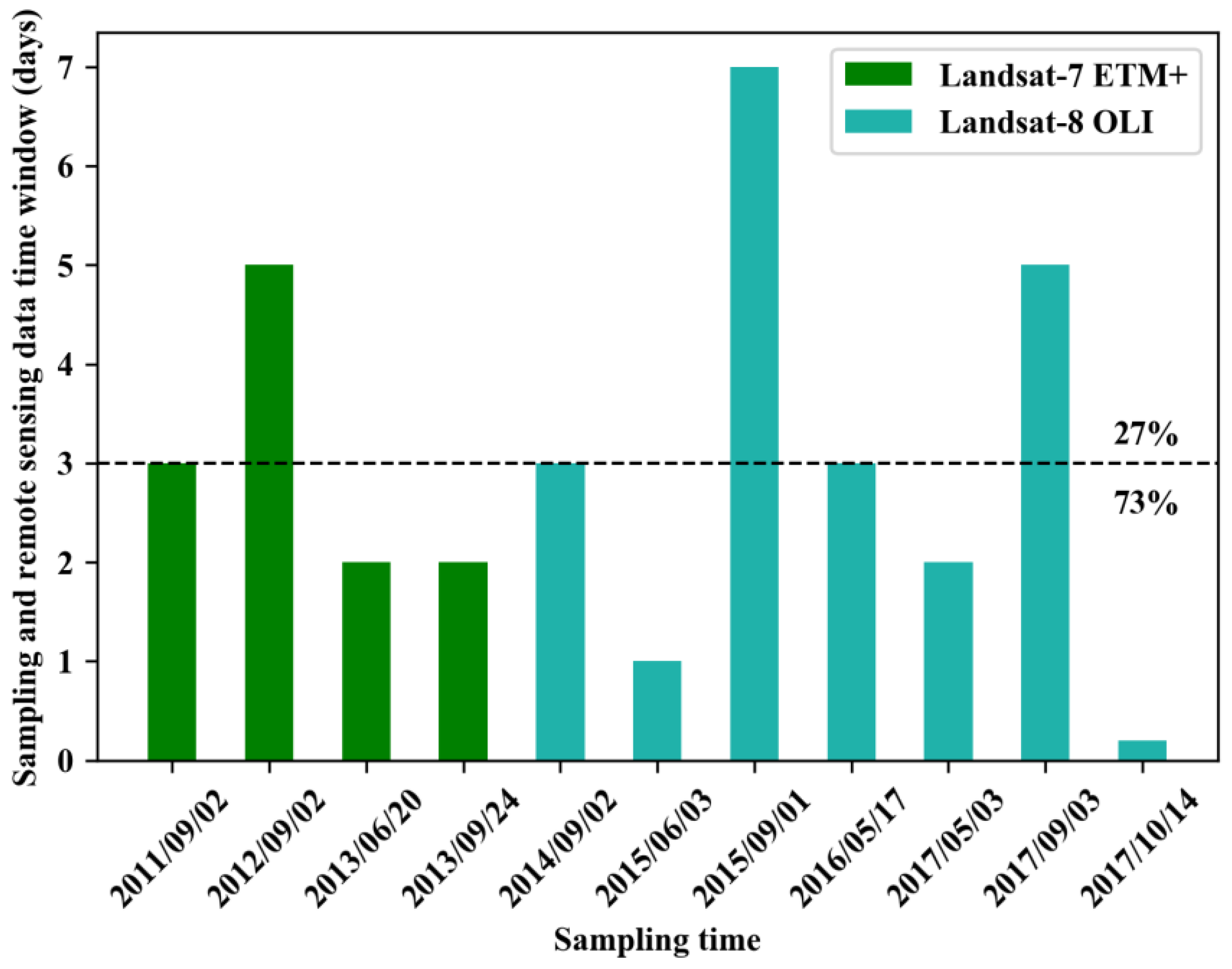
2.2. Data Acquisition and Processing
3. Methods
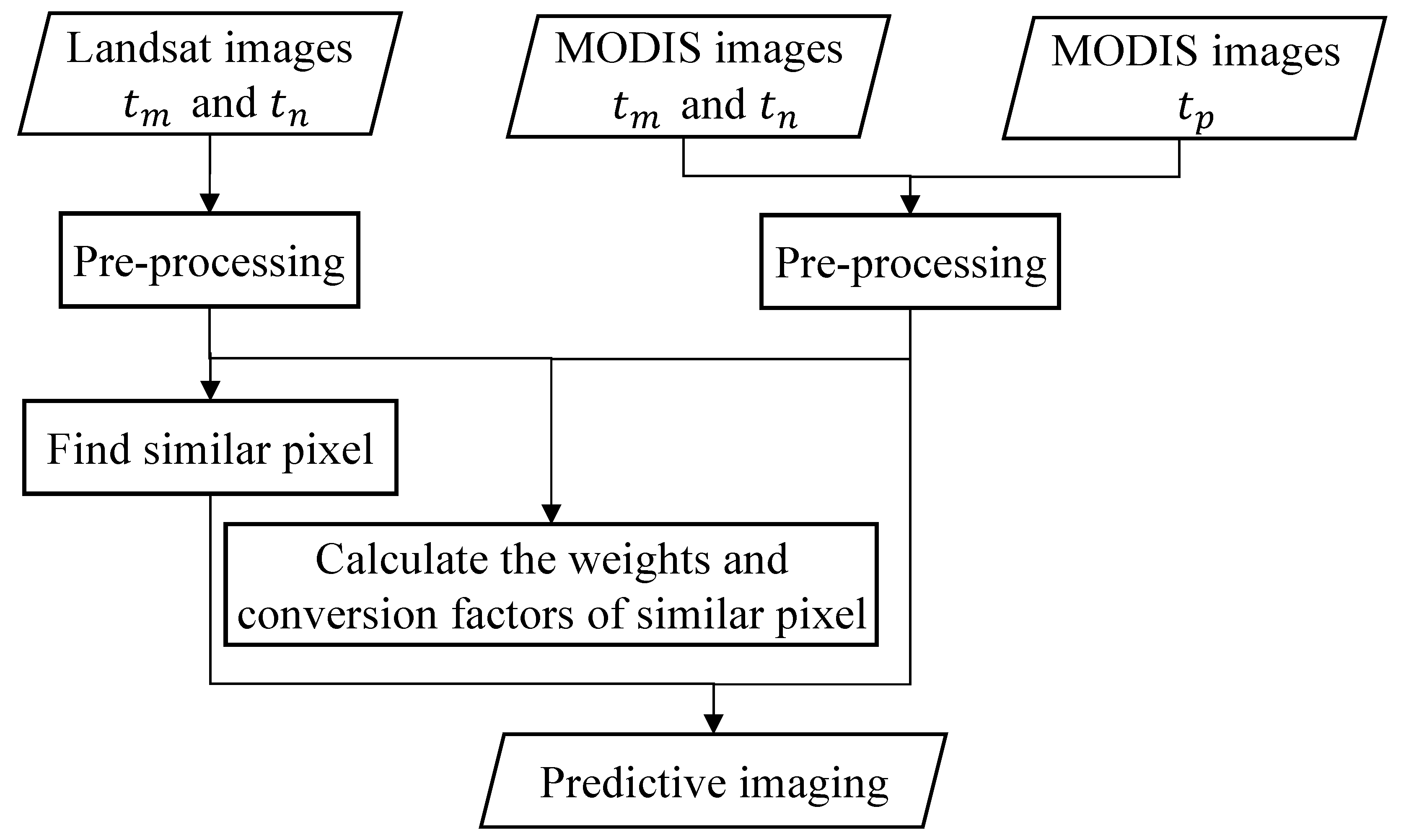
3.1. ESTARFM Algorithm
3.2. SPM Inversion Algorithm
- (1)
- Standardized data matrix X and Y of dependent variable were processed, and the obtained standardized matrices were expressed as E0 and F0, respectively.
- (2)
- The first pair of components of E0 and F0, t1 and u1, are linear combinations of standardized variables E0 and F0, respectively, and t1 requires maximum correlation to u1; then, the regression equations of E0 and F0 on t1 are obtained, and the residual matrix E1 and F1 of the regression equation can be obtained. E0 is replaced by E1, and F0 is replaced by F1. The second principal component t2 is obtained by the same method, and the nth principal component (n is less than the rank of matrix X) can be obtained.
- (3)
- Convergence is checked to determine the number of principal components extracted.
3.3. SPM Inversion Model Construction
3.4. Evaluation of Spatiotemporal Fusion Image Accuracy
3.5. Inversion Model Stability and Accuracy Evaluation
4. Results and Analysis
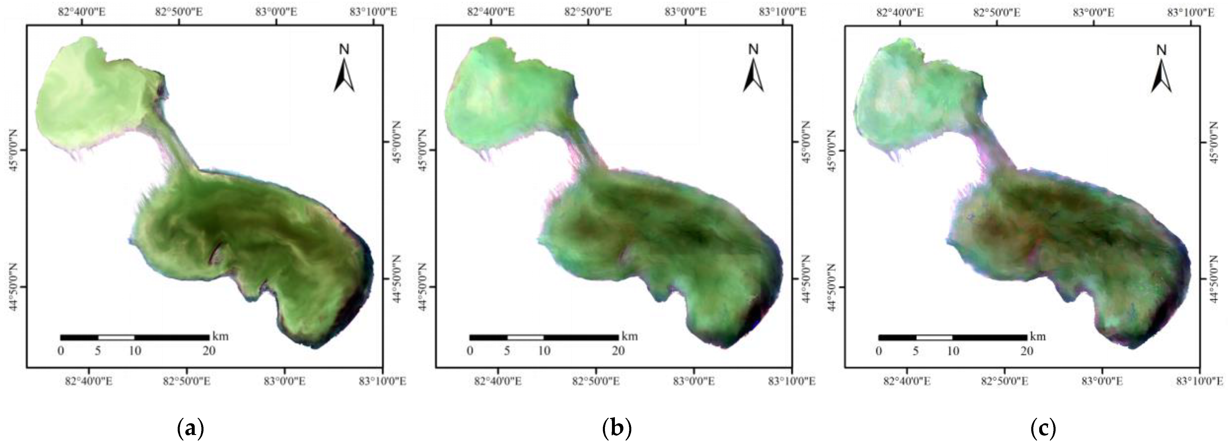
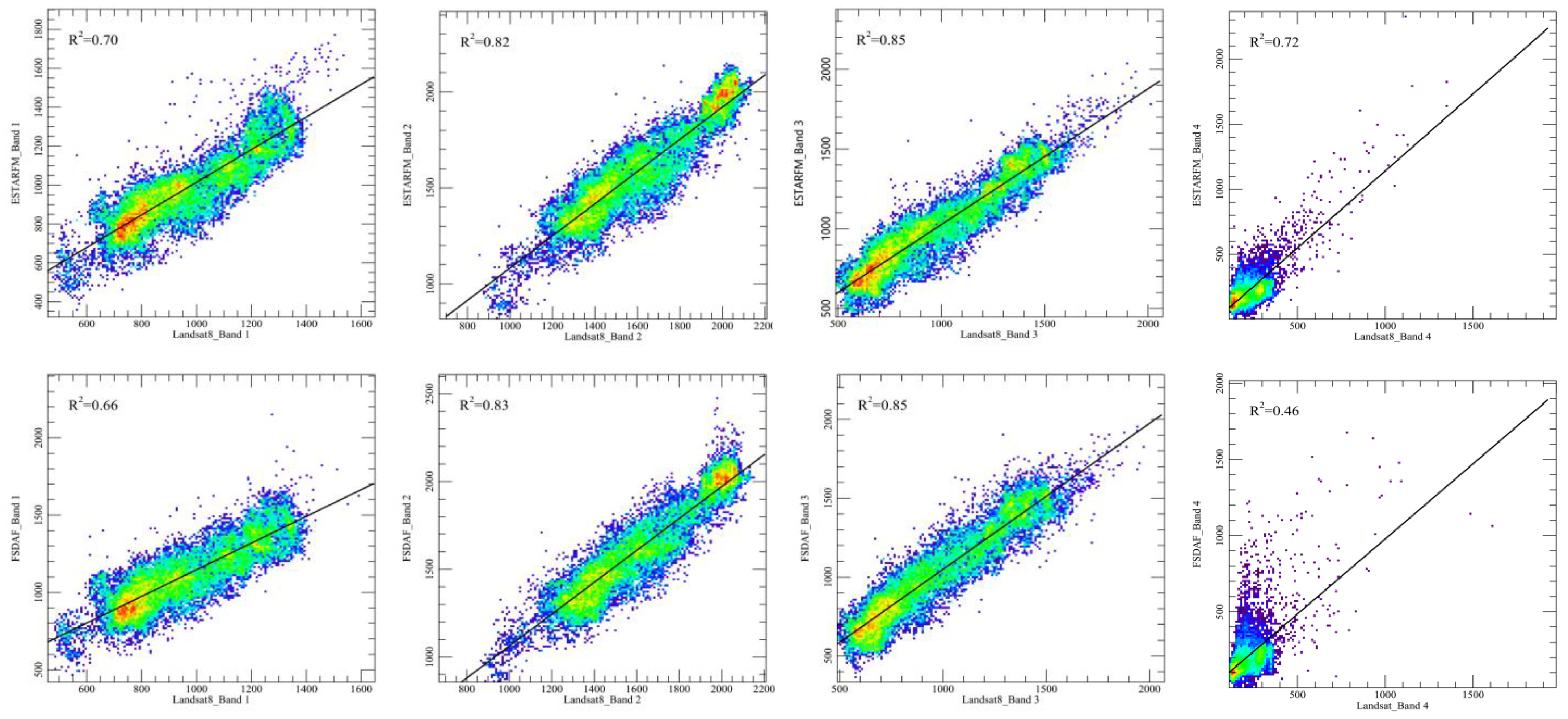
4.1. Performance Evaluation of the Spatiotemporal Fusion Model
4.2. SPM Inversion Model
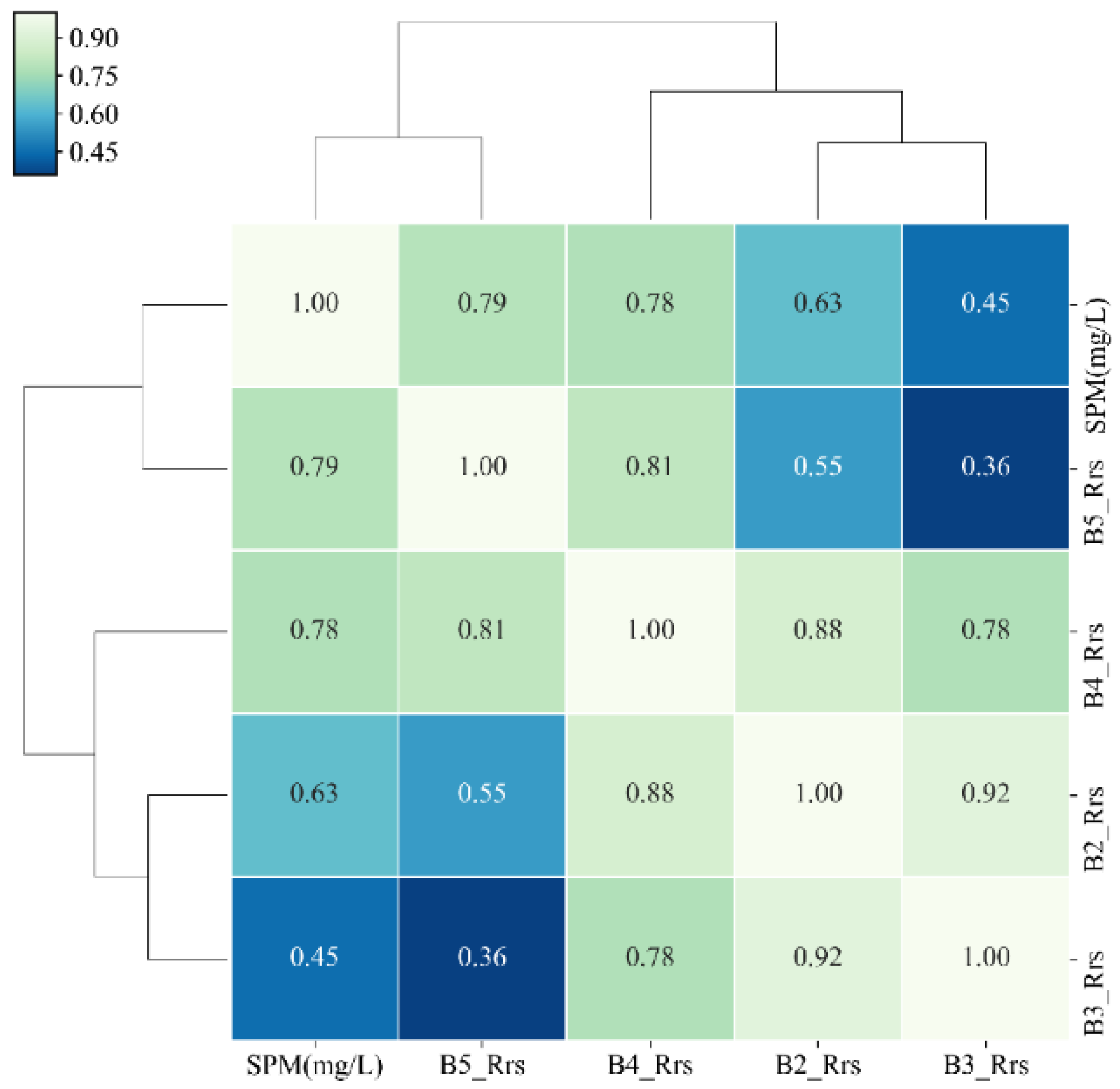
4.2.1. Screening of Sensitive Bands
4.2.2. SPM Inversion Model Performance
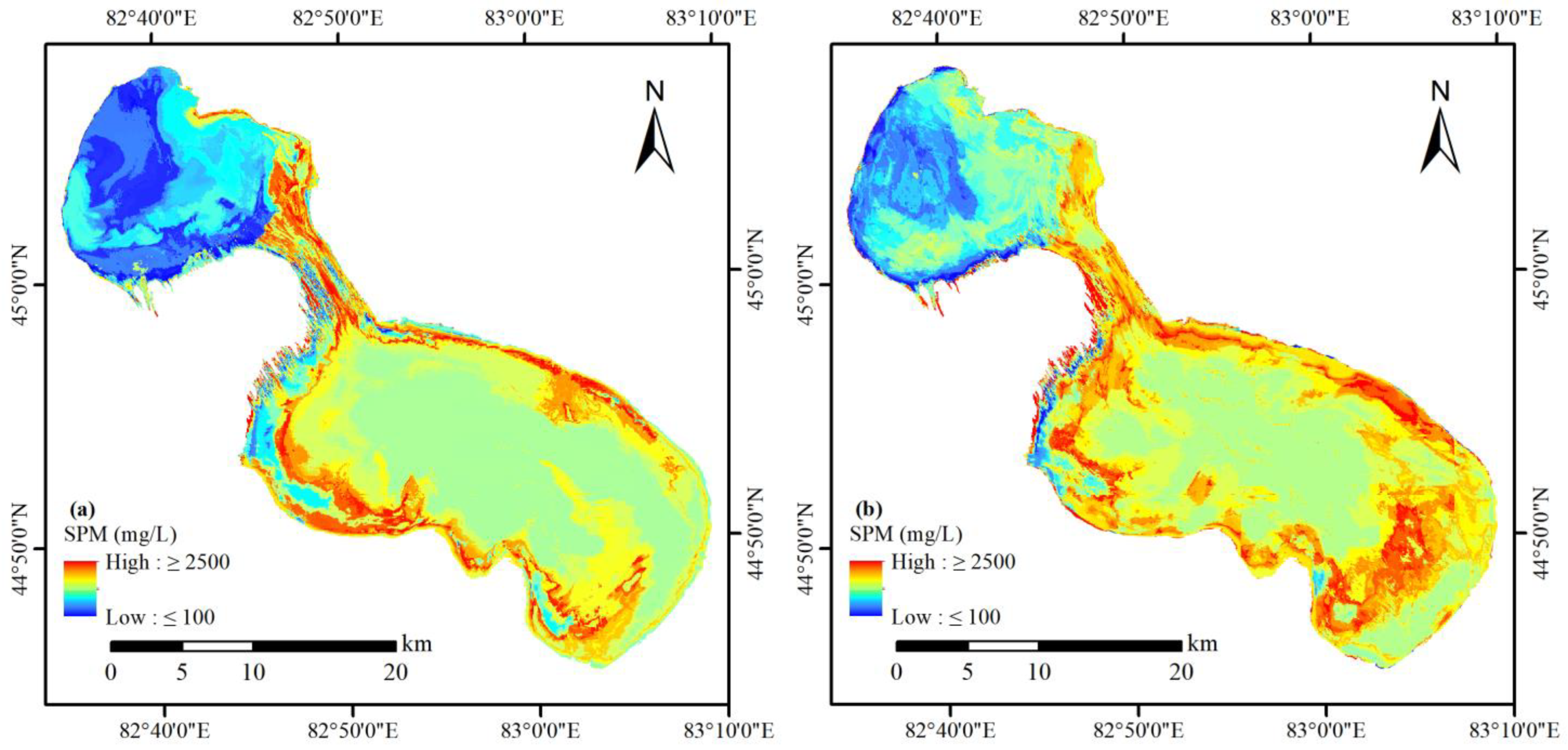
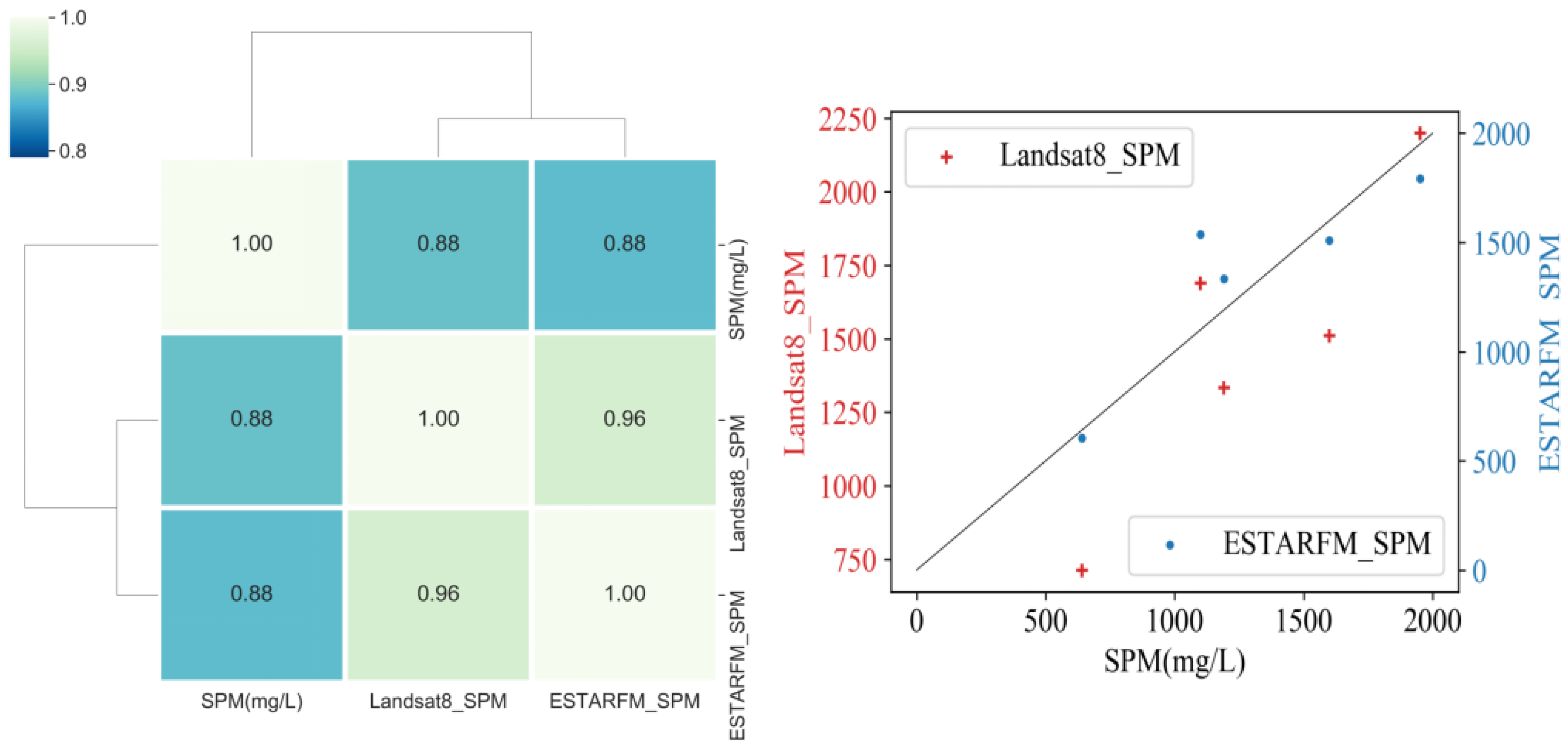
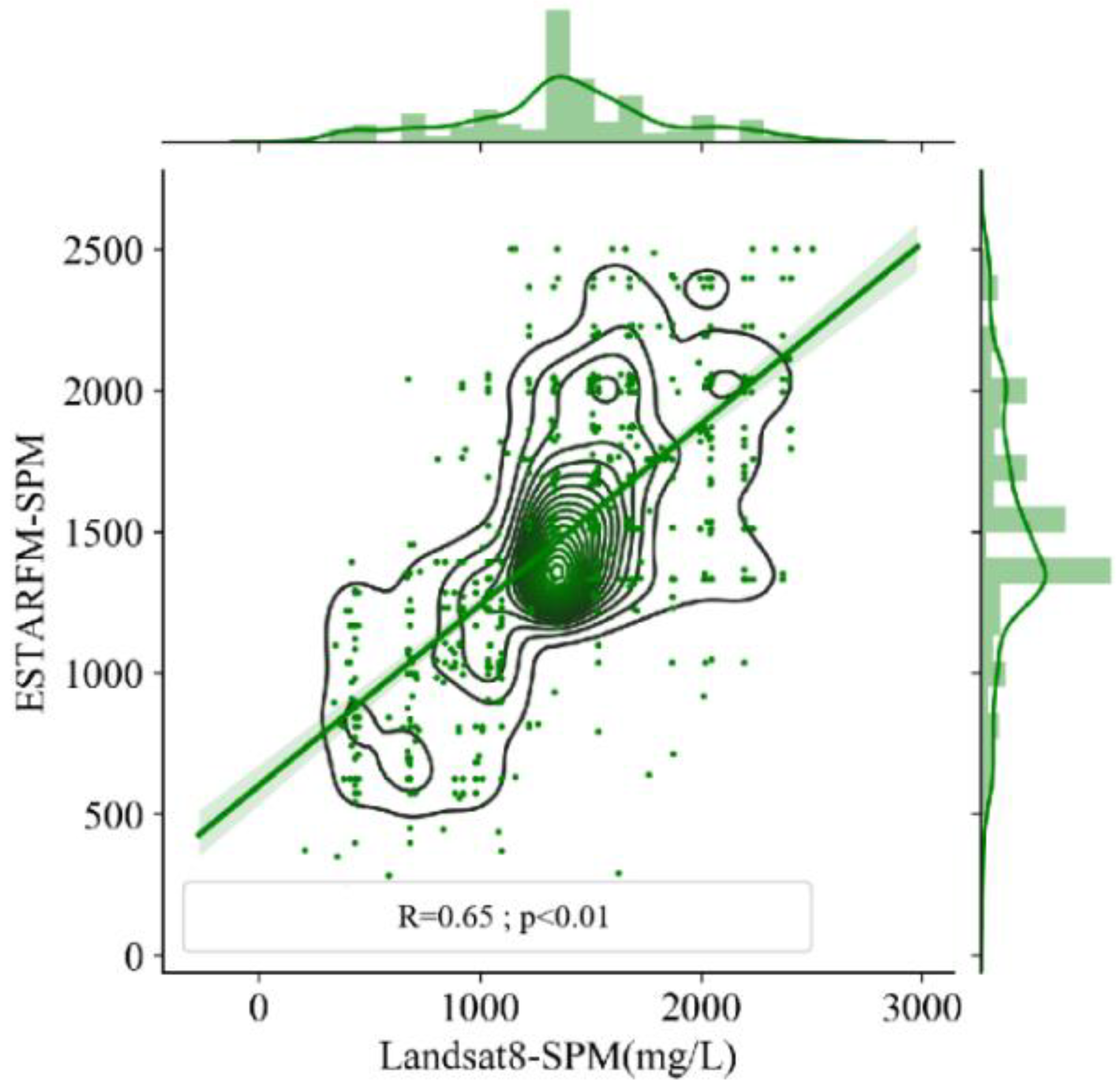
4.3. SPM Inversion Performance of Spatiotemporal Fusion Images
5. Discussion
6. Conclusions
- (1)
- The overall results of the blue, green, red, and NIR bands generated by ESTARFM were better than FSDAF when compared with the real images.
- (2)
- The RF inversion models based on Landsat images were proven to be better than PLS and SVM.
- (3)
- The visual perspective and accuracy assessment showed some consistency in the SPM concentration retrieved from the fused images of Landsat 8 and ESTARFM.
Author Contributions
Funding
Data Availability Statement
Acknowledgments
Conflicts of Interest
References
- Xu, Z.Q.; Shen, J.; Qu, Y.Q.; Chen, H.F.; Zhou, X.L.; Hong, H.C.; Sun, H.J.; Lin, H.J.; Deng, W.J.; Wu, F.Y. Using simple and easy water quality parameters to predict trihalomethane occurrence in tap water. Chemosphere 2022, 286, 131586. [Google Scholar] [CrossRef]
- Wang, J.; Sheng, Y.; Tong, T. Monitoring decadal lake dynamics across the Yangtze Basin downstream of Three Gorges Dam. Remote Sens. Environ. 2014, 152, 251–269. [Google Scholar] [CrossRef]
- Hou, X.; Feng, L.; Duan, H.; Chen, X.; Sun, D.; Shi, K. Fifteen-year monitoring of the turbidity dynamics in large lakes and reservoirs in the middle and lower basin of the Yangtze River, China. Remote Sens. Environ. 2017, 190, 107–121. [Google Scholar] [CrossRef]
- Zhu, S.D.; Zhang, F.; Zhang, Z.Y.; Kung, H.; Yushanjiang, A. Hydrogen and Oxygen Isotope Composition and Water Quality Evaluation for Different Water Bodies in the Ebinur Lake Watershed, Northwestern China. Water 2019, 11, 2067. [Google Scholar] [CrossRef] [Green Version]
- Sagan, V.; Peterson, K.T.; Maimaitijiang, M.; Sidike, P.; Sloan, J.; Greeling, B.A.; Maalouf, S.; Adams, C. Monitoring inland water quality using remote sensing: Potential and limitations of spectral indices, bio-optical simulations, machine learning, and cloud computing. Earth-Sci. Rev. 2020, 205, 103187. [Google Scholar] [CrossRef]
- Sun, Z.; Li, J.; Tian, L.; Cehn, B.; Hu, X. Spatial Variation and Risk Assessment of Arsenic and Heavy Metals in Surface Water and Suspended Particulate Matter in Tail Reaches of the Yellow River, China. Chin. Geogr. Sci. 2021, 31, 181–196. [Google Scholar] [CrossRef]
- Cao, Q.; Yu, G.; Qiao, Z. Application and recent progress of inland water monitoring using remote sensing techniques. Environ. Monit. Assess. 2023, 195, 1–16. [Google Scholar] [CrossRef]
- Ho, C.R.; Liu, A.K. Preface: Remote Sensing Applications in Ocean Observation. Remote Sens. 2023, 15, 415. [Google Scholar] [CrossRef]
- Chen, J.; Chen, S.; Fu, R.; Li, D.; Jiang, H.; Wang, C.; Peng, Y.; Jia, K.; Hicks, B.J. Remote sensing big data for water environment monitoring: Current status, challenges, and future prospects. Earth’s Future 2022, 10, e2021EF002289. [Google Scholar] [CrossRef]
- Lv, H.; Jiang, N.; Li, X.G. The Study on Water Quality of in Land Lake Monitoring by Remote Sensing. Adv. Earth Sci. 2005, 20, 185–192. [Google Scholar]
- Chen, C.; Mao, Z.H.; Tang, F.P.; Han, G.Q.; Jiang, Y.Z. Declining riverine sediment input impact on spring phytoplankton bloom off the Yangtze River Estuary from 17-year satellite observation. Cont. Shelf Res. 2017, 135, 86–91. [Google Scholar] [CrossRef]
- Lee, Z.; Carder, K.L.; Arnone, R.A. Deriving inherent optical properties from water color: A multiband quasi-analytical algorithm for optically deep waters. Appl. Opt. 2002, 41, 5755–5772. [Google Scholar] [CrossRef]
- Rotta, L.; Alcântara, E.; Park, E.; Bernardo, N.; Watanabe, F. A single semi-analytical algorithm to retrieve chlorophyll-a concentration in oligo-to-hypereutrophic waters of a tropical reservoir cascade. Ecol. Indic. 2021, 120, 106913. [Google Scholar] [CrossRef]
- Lu, H.F.; Ma, X. Hybrid decision tree-based machine learning models for short-term water quality prediction. Chemosphere 2020, 249, 126169. [Google Scholar] [CrossRef]
- Sun, J.; Zhong, G.; Huang, K.; Dong, J. Banzhaf random forests: Cooperative game theory based random forests with consistency. Neural Netw. 2018, 106, 20–29. [Google Scholar] [CrossRef]
- Grimm, R.; Behrens, T.; Märker, M.; Elsenbeer, H. Soil organic carbon concentrations and stocks on Barro Colorado Island-Digital soil mapping using Random Forests analysis. Geoderma 2008, 146, 102–113. [Google Scholar] [CrossRef]
- Su, Z.H.; Chen, L.; Ma, R.H.; Luo, J.H.; Liang, Q.O. Effect of land use change on lake water quality in different buffer zones. Appl. Ecol. Environ. Res. 2015, 13, 639–653. [Google Scholar]
- Dube, T.; Shekede, M.D.; Massari, C. Remote sensing for water resources and environmental management. Remote Sens. 2023, 15, 18. [Google Scholar] [CrossRef]
- Huang, Z.; Li, Y.; Bai, M.; Wei, Q.; Gu, Q.; Mou, Z.; Zhang, L.; Lei, D. A Multiscale Spatiotemporal Fusion Network Based on an Attention Mechanism. Remote Sens. 2023, 15, 182. [Google Scholar] [CrossRef]
- Zhu, X.; Cai, F.; Tian, J.; Williams, T.K.A. Spatiotemporal fusion of multisource remote sensing data: Literature survey, taxonomy, principles, applications, and future directions. Remote Sens. 2018, 10, 527. [Google Scholar] [CrossRef] [Green Version]
- Liang, Z.H. Research on the Construction of Tasseled Cap Transform Indices Time Series Data Sets Based on Spatial-Temporal Fusion Algorithm; Lanzhou University: Lanzhou, China, 2015. (In Chinese) [Google Scholar]
- Sun, L.; Gao, F.; Xie, D.; Anderson, M.; Chen, R.; Yang, Y.; Yang, Y.; Chen, Z. Reconstructing daily 30m NDVI over complex agricultural landscapes using a crop reference curve approach. Remote Sens. Environ. 2020, 253, 112156. [Google Scholar] [CrossRef]
- Gao, F.; Masek, J.; Schwaller, M.; Hall, F. On the blending of the Landsat and MODIS surface reflectance: Predicting daily Landsat surface reflectance. IEEE Trans. Geosci. Remote Sens. 2006, 44, 2207–2218. [Google Scholar]
- Zhu, X.; Chen, J.; Gao, F.; Chen, X.; Masek, J.G. An enhanced spatial and temporal adaptive reflectance fusion model for complex heterogeneous regions. Remote Sens. Environ. 2010, 114, 2610–2623. [Google Scholar] [CrossRef]
- Cheng, Q.; Liu, H.; Shen, H.; Wu, P.; Zhang, L. A Spatial and Temporal Nonlocal Filter-Based Data Fusion Method. IEEE Trans. Geosci. Remote Sens. 2017, 55, 4476–4488. [Google Scholar] [CrossRef] [Green Version]
- Xie, D.; Zhang, J.; Zhu, X.; Pan, Y.; Liu, H.; Yuan, Z.; Yun, Y. An improved STARFM with help of an unmixing-based method to generate high spatial and temporal resolution remote sensing data in complex heterogeneous regions. Sensors 2016, 16, 207. [Google Scholar] [CrossRef] [Green Version]
- Zhu, X.; Helmer, E.H.; Gao, F.; Liu, D.; Chen, J.; Lefsky, M.A. A flexible spatiotemporal method for fusing satellite images with different resolutions. Remote Sens. Environ. 2016, 172, 165–177. [Google Scholar] [CrossRef]
- Huang, B.; Song, H. Spatiotemporal Reflectance Fusion via Sparse Representation. IEEE Trans. Geosci. Remote Sens. 2012, 50, 3707–3716. [Google Scholar] [CrossRef]
- Wang, L.; Li, Y.; Wang, Y.; Guo, J.; Xia, Q.; Tu, Y.; Nie, P. Compensation benefits allocation and stability evaluation of cascade hydropower stations based on Variation Coefficient -Shapley Value Method. J. Hydrol. 2021, 599, 126277. [Google Scholar] [CrossRef]
- Li, P.; Ke, Y.; Wang, D.; Ji, H.; Chen, S.; Chen, M.; Lyu, M.; Zhou, D. Human impact on suspended particulate matter in the Yellow River Estuary, China: Evidence from remote sensing data fusion using an improved spatiotemporal fusion method. Sci. Total Environ. 2021, 750, 141612. [Google Scholar] [CrossRef]
- Liu, C.J.; Duan, P.; Zhang, F.; Jim, C.Y.; Tan, M.L.; Chan, N.W. Feasibility of the Spatiotemporal Fusion Model in Monitoring Ebinur Lake’s Suspended Particulate Matter under the Missing-Data Scenario. Remote Sens. 2021, 13, 3952. [Google Scholar] [CrossRef]
- GB11901-89; Water Quality Determination of Suspended Substance-Gravimetric Method. Peoples’ Republic of China: Beijing, China, 1989.
- Cao, Z.; Duan, H.; Song, Q.; Shen, M.; Ma, R.; Liu, D. Evaluation of the sensitivity of China’s next-generation ocean satellite sensor MWI onboard the Tiangong-2 space lab over inland waters. Int. J. Appl. Earth Obs. Geoinf. 2018, 71, 109–120. [Google Scholar] [CrossRef]
- Manoj, K.M.; Bimal, B. 4-Atmospheric parameter retrieval and correction using hyperspectral data. Hyperspectral Remote Sens. 2020, 67–84. [Google Scholar] [CrossRef]
- Watson, C.S.; King, O.; Miles, E.S.; Quincey, D.J. Optimising NDWI supraglacial pond classification on Himalayan debris-covered glaciers. Remote Sens. Environ. 2018, 217, 414–425. [Google Scholar] [CrossRef]
- Wold, S.; Ruhe, A.; Wold, H.; Dunn, W.J., III. The Collinearity Problem in Linear Regression. The Partial Least Squares (PLS) Approach to Generalized Inverse. SLAM J. Sci. Stat. Comput. 1984, 5, 735–743. [Google Scholar] [CrossRef] [Green Version]
- Rosipal, R.; Kramer, N. Overview and Recent Advances in Partial Least Squares. In Subspace, Latent Structure and Feature Selection, Bohinj, Slovenia, 23–25 February 2005; Springer: Berlin/Heidelberg, Germany, 2006; pp. 34–51. [Google Scholar]
- Wold, S.; Sjöström, M.; Eriksson, L. PLS-regression: A basic tool of chemometrics. Chemom. Intell. Lab. Syst. 2001, 58, 109–130. [Google Scholar] [CrossRef]
- Huang, W. Diagnosis and Solution of Collinearity in Multiple Regression Modeling; Harbin Institute of Technology: Harbin, China, 2012. (In Chinese) [Google Scholar]
- Chen, J.H.; Yu, H.L.; Jiang, D.P.; Zhang, Y.Z.; Wang, K.Q. A novel NIRS modelling method with OPLS-SPA and MIX-PLS for timber evaluation. J. For. Res. 2022, 33, 369–376. [Google Scholar] [CrossRef]
- Joachims, T. Making Large-Scale SVM Learning Practical. Tech. Rep. 1988, 8, 499–526. [Google Scholar]
- Breiman, L. Random forests. Mach. Learn. 2001, 45, 5–32. [Google Scholar] [CrossRef] [Green Version]
- Breiman, L. Bagging predictors. Mach. Learn. 1996, 24, 123–140. [Google Scholar] [CrossRef] [Green Version]
- Sun, J.Y.; Wang, G.Z.; He, G.J.; Pu, D.C.; Jiang, W.; Li, T.T.; Niu, X.F. Study on the water body extraction using GF-1 data based on adaboost integrated learning algorithm. Int. Arch. Photogramm. Remote Sens. Spat. Inf. Sci. 2020, 42, 641–648. [Google Scholar] [CrossRef] [Green Version]
- Ho, T.K. The random subspace method for constructing decision forests. IEEE Trans. Pattern Anal. Mach. Intell. 1998, 20, 832–844. [Google Scholar]
- Wang, Y.S.; Xia, S.T. A survey of random forests algorithms. Inf. Commun. Technol. 2018, 12, 49–55. [Google Scholar]
- Fang, X.; Wen, Z.; Chen, J.; Wu, S.; Huang, Y.; Ma, M. Remote sensing estimation of suspended sediment concentration based on Random Forest Regression Model. J. Remote Sens. 2019, 23, 756–772. [Google Scholar]
- Wang, Z. Image Quality Assessment: From Error Visibility to Structural Similarity. IEEE Trans. Image Process. 2004, 13, 600–612. [Google Scholar] [CrossRef] [Green Version]
- Horé, A.; Ziou, D. Image quality metrics: PSNR vs. SSIM. In Proceedings of the 2010 20th International Conference on Pattern Recognition, Istanbul, Turkey, 23–26 August 2010; pp. 2366–2369. [Google Scholar] [CrossRef]
- Klein, G.A. A recognition-primed decision (RPD) model of rapid decision making. Decis. Mak. Action Model. Methods 1993, 5, 138–147. [Google Scholar]
- Chang, C.W.; Laird, D.A.; Mausbach, M.J.; Hurburgh, C.R. Near-Infrared Reflectance Spectroscopy-Principal Components Regression Analyses of Soil Properties. Soil Sci. Soc. Am. J. 2001, 65, 480–490. [Google Scholar] [CrossRef] [Green Version]
- Yuan, J.; Wang, X.; Yan, C.X.; Wang, S.R.; Ju, X.P.; Li, Y. Soil Moisture Retrieval Model for Remote Sensing Using Reflected Hyperspectral Information. Remote Sens. 2019, 11, 366. [Google Scholar] [CrossRef] [Green Version]
- Amin, I.; Fikrat, F.; Mammadov, E.; Babayev, M. Soil organic carbon prediction by Vis-NIR Spectroscopy: Case Study the Kur-Aras Plain, Azerbaijan. Commun. Soil Sci. Plant Anal. 2020, 51, 1–9. [Google Scholar] [CrossRef]
- Fu, D.; Chen, B.; Wang, J.; Zhu, X.; Hilker, T. An improved image fusion approach based on enhanced spatial and temporal the adaptive reflectance fusion model. Remote Sens. 2013, 5, 6346–6360. [Google Scholar] [CrossRef] [Green Version]
- Zhang, X.C.; Wang, J. The Analysis of Eco-hydrological Structure of Shengjin Lake Wetland based on Spatial and Temporal Fusion Technology of Remote Sensing. Remote Sens. Technol. Appl. 2020, 35, 1109–1117. [Google Scholar]
- Doña, C.; Chang, N.B.; Caselles, V.; Sánchez, J.M.; Camacho, A.; Delegido, J.; Vannah, B.W. Integrated satellite data fusion and mining for monitoring lake water quality status of the Albufera de Valencia in Spain. J. Environ. Manag. 2015, 151, 416–426. [Google Scholar] [CrossRef] [Green Version]
- Carpenter, D.J.; Carpenter, S.M. Modeling inland water quality using Landsat data. Remote Sens. Environ. 1983, 13, 345–352. [Google Scholar] [CrossRef]
- Dörnhöfer, K.; Oppelt, N. Remote sensing for lake research and monitoring-Recent advances. Ecol. Indic. 2016, 64, 105–122. [Google Scholar] [CrossRef]
- Shen, C. A transdisciplinary review of deep learning research and its relevance for water resources scientists. Water Resour. Res. 2018, 54, 8558–8593. [Google Scholar] [CrossRef]
- Shah, S.H.; Angel, Y.; Houborg, R.; Ali, S.; McCabe, M.F. A random forest machine learning approach for the retrieval of leaf chlorophyll content in wheat. Remote Sens. 2019, 11, 920. [Google Scholar] [CrossRef] [Green Version]
- Guan, Q.H.; Ding, M.J.; Zhang, H.; Wang, P. Analysis of applicability about ESTARFM in the middle-lower Yangtze Plain. J. Geo-Inf. Sci. 2021, 23, 1118–1130. [Google Scholar]
- Yang, H.; Du, Y.; Zhao, H.; Chen, F. Water quality Chl-a inversion based on spatio-temporal fusion and convolutional neural network. Remote Sens. 2022, 14, 1267. [Google Scholar] [CrossRef]
- Nazirova, K.; Alferyeva, Y.; Lavrova, O.; Shur, Y.; Soloviev, D.; Bocharova, T.; Strochkov, A. Comparison of in situ and remote-sensing methods to determine turbidity and concentration of suspended matter in the estuary zone of the mzymta river, black sea. Remote Sens. 2021, 13, 143. [Google Scholar] [CrossRef]
- Kim, Y.W.; Kim, T.; Shin, J.; Lee, D.S.; Park, Y.S.; Kim, Y.; Cha, Y. Validity evaluation of a machine-learning model for chlorophyll a retrieval using Sentinel-2 from inland and coastal waters. Ecol. Indic. 2022, 137, 108737. [Google Scholar] [CrossRef]


| Max (mg/L) | Min (mg/L) | Mean (mg/L) | Std (mg/L) | |
|---|---|---|---|---|
| SPM (n = 42) | 8350.00 | 18.50 | 1395.32 | 2376.33 |
| Landsat 8 | Spatiotemporal Resolution | MOD09GA | Spatiotemporal Resolution | Prediction Time |
|---|---|---|---|---|
| 2017-05-08 | 30 m/16 d | 2017-05-08 | 500 m/1 d | 2017-08-28 (30 m) |
| 2017-08-28 | 2017-08-29 | |||
| 2017-10-15 | 2017-10-14 |
| Band | R2 | NRMSE | PSNR | SSIM | ||||
|---|---|---|---|---|---|---|---|---|
| ESTARFM | FSDAF | ESTARFM | FSDAF | ESTARFM | FSDAF | ESTARFM | FSDAF | |
| Blue | 0.70 | 0.66 | 0.13 | 0.21 | 48.26 | 44.02 | 0.61 | 0.53 |
| Green | 0.82 | 0.83 | 0.08 | 0.08 | 48.44 | 48.48 | 0.70 | 0.70 |
| Red | 0.85 | 0.85 | 0.12 | 0.13 | 48.22 | 47.64 | 0.75 | 0.71 |
| NIR | 0.72 | 0.46 | 0.42 | 0.59 | 49.23 | 46.22 | 0.62 | 0.45 |
| Remote Sensing Image | Evaluation Indicator | PLS | SVM | RF | |||
|---|---|---|---|---|---|---|---|
| Training Set | Verification Set | Training Set | Verification Set | Training Set | Verification Set | ||
| Landsat 8 | R2 | 0.79 | 0.57 | 0.65 | 0.50 | 0.92 | 0.78 |
| RMSE | 1420.90 | 2530.50 | 1873.64 | 2750.76 | 870.75 | 1823.64 | |
| MAE | 1175.51 | 1495.02 | 1072.62 | 1448.06 | 587.39 | 1026.36 | |
| RPD | 1.55 | 1.41 | 2.13 | ||||
Disclaimer/Publisher’s Note: The statements, opinions and data contained in all publications are solely those of the individual author(s) and contributor(s) and not of MDPI and/or the editor(s). MDPI and/or the editor(s) disclaim responsibility for any injury to people or property resulting from any ideas, methods, instructions or products referred to in the content. |
© 2023 by the authors. Licensee MDPI, Basel, Switzerland. This article is an open access article distributed under the terms and conditions of the Creative Commons Attribution (CC BY) license (https://creativecommons.org/licenses/by/4.0/).
Share and Cite
Zhang, F.; Duan, P.; Jim, C.Y.; Johnson, V.C.; Liu, C.; Chan, N.W.; Tan, M.L.; Kung, H.-T.; Shi, J.; Wang, W. An Advanced Spatiotemporal Fusion Model for Suspended Particulate Matter Monitoring in an Intermontane Lake. Remote Sens. 2023, 15, 1204. https://doi.org/10.3390/rs15051204
Zhang F, Duan P, Jim CY, Johnson VC, Liu C, Chan NW, Tan ML, Kung H-T, Shi J, Wang W. An Advanced Spatiotemporal Fusion Model for Suspended Particulate Matter Monitoring in an Intermontane Lake. Remote Sensing. 2023; 15(5):1204. https://doi.org/10.3390/rs15051204
Chicago/Turabian StyleZhang, Fei, Pan Duan, Chi Yung Jim, Verner Carl Johnson, Changjiang Liu, Ngai Weng Chan, Mou Leong Tan, Hsiang-Te Kung, Jingchao Shi, and Weiwei Wang. 2023. "An Advanced Spatiotemporal Fusion Model for Suspended Particulate Matter Monitoring in an Intermontane Lake" Remote Sensing 15, no. 5: 1204. https://doi.org/10.3390/rs15051204