
Non-Ellipsoidal Infrared Group/Extended Target Tracking Based on Poisson Multi-Bernoulli Mixture Filter and B-Spline

1
Shanghai Institute of Technical Physics, Chinese Academy of Sciences, Shanghai 200083, China
2
Key Laboratory of Intelligent Infrared Perception, Chinese Academy of Sciences, Shanghai 200083, China
3
University of Chinese Academy of Sciences, Beijing 100049, China
*
Author to whom correspondence should be addressed.
Remote Sens. 2023, 15(3), 606; https://doi.org/10.3390/rs15030606
Submission received: 17 November 2022
/
Revised: 4 January 2023
/
Accepted: 17 January 2023
/
Published: 19 January 2023
Abstract
:This study provides a solution for multiple group/extended target tracking with an arbitrary shape. Many tracking approaches for extended/group targets have been proposed. However, these approaches make assumptions about the target shape, which have limitations in practical applications. To address this problem, in this work, an extended/group target tracking algorithm based on B-spline is proposed. Specifically, the extension of an extended or a group target was modeled as a spatial probability distribution characterized by the control points of a B-spline function that was then jointly propagated with the measurement rate model and kinematic component model over time using the Poisson multi-Bernoulli mixture (PMBM) filter framework. In addition, an amplitude-aided measurement partitioning approach is proposed to improve the accuracy caused by distance-based approaches. The simulation results demonstrate that the extension, shape and orientation of targets can be estimated better by the proposed algorithm, even if the shape changes. The tracking performance is also improved by about 10% and 13% compared to the other two algorithms.
1. Introduction
With the increase in human space activities, the number of space targets, including debris, abandoned spacecraft, missiles, and so forth is also increasing, thus affecting the safety of human space activities. This study focuses on tracking space targets based on space-based infrared sensors. Tracking problems related to space targets are part of the multi-target tracking problem. Multi-target tracking (MTT) is a hot topic both in military and civilian fields [1,2]. Most traditional tracking algorithms are based on the assumption that each target produces at most one measurement per time step limited by the resolution of the traditional sensors. However, with the rapid development of sensors, the resolution and accuracy have been greatly improved. Thus, the assumption no longer holds; that is, a target may generate multiple measurements at a given time. In this case, the target is preferably treated as an extended target [3] with a specific size, shape and orientation. When targets are close enough, they form an invisible group target, which acts as an extended target; therefore, the tracking of a group target can be regarded as the tracking of an extended target [4]. Generally, the tracking process of multiple group/extended targets contains three steps. Firstly, the target state is modeled. Secondly, the data received from sensors are processed, which involves partitioning the measurements, and data are associated with the measurements and the targets. Lastly, the iterative state parameters containing the predictions and updated processes of the parameters are outlined. The discussion that follows focuses on extended target tracking, which can also be applied to group targets.
There are two models that can be considered for extended targets: (1) a model of the number of measurements generated by each extended target and (2) a model of the spatial distribution of the targets. Generally, the number of measurements generated by the extended target is modeled using the Poisson distribution, whose rate parameter is modeled as a gamma distribution [5]. As for the target extension, it is critical for target identification in the tracking scenario and is the focus of the present study. It has been the subject of many studies.
When it comes to target extension, there are two assumptions in the literature: (1) the assumption that there are some general parameters that can describe the shape of the targets, such as an ellipse, rectangle [6], line [7], and so on, and (2) the assumption of an arbitrary shape. For the former, an ellipse is the most frequently used, and there are several approaches for ellipse modeling, such as random matrix (RM) [8] theory, which models the extension as a symmetric positive definite matrix. Generally, the gamma Gaussian inverse–Wishart (GGIW) distribution [5,9,10,11] is adapted. In these cases, the extended target is assumed to be elliptical. These methods are effective and have been applied to many scenarios [9]. However, their performance suffers when the shape is not elliptical. To estimate the non-elliptical extended target, [4,12] modeled the extension of the arbitrary shape using multiple ellipses (Em) and achieved the tracking of non-elliptical extended targets. However, a priori knowledge of the number of ellipses is needed. When the actual shape is unknown, it is challenging to choose an appropriate number of ellipses. To more accurately estimate the shape of the targets, random hypersurface models (RHMs) [13] were proposed by Baum. The shape constraint (i.e., elliptical constraint, star-convex constraint and level-set constraint) needs to be set to describe the target-extended state. That is, the extension can be obtained by estimating the parameters of the shape constraint. RHMs outperform RM models and can estimate extended targets with an irregular shape when using accurate preset shape constraints, but the computational complexity is higher. Many scholars have made great improvements based on these models. However, these methods all require assumptions about the shape of the target. In addition, some scholars have proposed other methods to estimate the shapes of extended targets. The extension–deformation approach [14] was proposed by Xiaorong to obtain the estimated shapes of targets. An extended target is considered to have a reference extension with control points on the boundary [14]. Then, the extension is estimated by moving some of the control points. The reference extension and the control points are a priori, which limits their application in practical scenarios due to the varying number of control points. Yulan Han applied an algorithm based on the level set and Gaussian surface fitting to extended target tracking [15]. Some researchers also use a B-spline curve to fit the shape [16,17]. A B-spline curve can be fitted to arbitrary shapes by adjusting the control points to estimate the shape of the extended target shape [17] assumed that the measurement points are generated using an edge, which is not applicable for some targets, especially group targets. In addition, non-uniform rational B-splines (NURBS) surfaces which can be considered as an extension of B-spline have been successfully applied to estimate a 3-dimensional (3D) target extension [18,19]. However, although NURBS is more flexible, it needs extra storage to define traditional curves and surfaces. In addition, weights have a significant impact on the shape estimation. Improper weights can cause shape distortion [20].
In addition, measurement partitioning is another important part of extended target tracking. Whether the measurement subset of each group target can be correctly divided at each specific moment determines the estimation accuracy of the group target state’s estimation accuracy and the tracking performance of the algorithm. Thus, distance partition, k-means ++ partition [21], prediction partition [22] and expectation maximization (EM) partition [21], DBSCAN [23] are proposed and successfully applied. However, the value of the distance threshold is difficult to determine. In addition, the distance information is insignificant in infrared images. For k-means ++, a priori knowledge of the selection and number of cluster centers is required. While the prediction information at the previous moment is inaccurate, such as the target maneuvering, the prediction partition and expectation maximization (EM) partition fail. For DBSCAN, the choice of two parameters is a challenge, and different parameter combinations have a significant effect on clustering. In addition, the performance degrades when the density of the sample set is not uniform. [23] proposed a grid-based DBSCAN algorithm which can deal with the non-equidistant sampling density and improve the performance. For infrared images, amplitude information is introduced to the partition measurements in this study.
Once models are defined, a multi-target filter is needed to implement the estimation of the target state, number and shape. To track multiple extended targets, random finite sets (RFSs) that model targets and measurements as random sets can provide an effective solution for data association and have received a great deal of attention in the literature. PMBM [24] and the Delta-generalized labeled multi-Bernoulli (-GLMB) [25] are two well-established MTT conjugate priors that have better performance than others. Meanwhile, the simulation results show that PMBM filters outperform -GLMB filters both in terms of their performance and computation cost [5,26]. Inspired by [16] and [5], in this study, a multiple extended target tracking algorithm based on B-spline and the PMBM filter is proposed. In addition, the amplitude-aided method is used for the measurement portioning part. Specifically, the target state is modeled in three parts. The first part denotes the number of measurements generated by an extended target, which is modeled using Poisson distribution, and the Poisson rate is modeled using gamma distribution. The second part is the kinematic state of the extended target center and is modeled using Gaussian distribution. The last part represents the extension of the extended targets and is modeled using a spatial probability distribution characterized by control points of a B-spline function. Then, the single target state is propagated by iterating parameters of models. Lastly, multi-target tracking is implemented under the PMBM filter.
This study focuses on tracking the multiple non-ellipsoidal targets based on the PMBM filter. There are three contributions of this work, which are as follows:
- (1)
- The B-spline is applied to model the extension of extended targets, thus solving the inaccurate modeling of targets with an arbitrary shape. In addition, the performance is also improved using this algorithm.
- (2)
- The amplitude information is introduced to partition the measurement, which can accurately partition the measurement set, especially when the targets are close.
- (3)
- The updated prediction and likelihood formulas of the algorithm based on the B-spline model are derived.
The remainder of the paper is organized as follows. In Section 2, the background of the proposed algorithm is provided. Section 3 provides the implementation of the proposed algorithm. Section 4 presents the numerical simulation to verify the proposed algorithm, and several methods are compared with the proposed algorithm. Section 5 provides the conclusion.
2. Background
This section provides the background on the implementation of the proposed algorithm.
2.1. PMBM Density
Once the models of kinematic state and extension and the number of measurements generated by an extended target are defined, the multiple extended target tracking algorithm can be proposed based on the models and the PMBM filter. The PMBM filter is a promising filter that models the undetected targets and the detected targets using a Poisson point process (PPP) and multi-Bernoulli mixture (MBM) process, respectively. Thus, the set of targets can be divided into two-joint subsets [27]:
where denotes the undetected targets and is the detected targets at time . The density can be expressed as
where denotes the Poisson density, denotes the intensity function of PPP, is the Poisson rate, represents the spatial distribution, and . is a mixture of multi-Bernoulli denoting the potential targets that are detected at least once. and are an index set for the multi-Bernoullis (MBs) in the MBM and an index set for the Bernoullis in the MB, respectively. is the number of MB components in the MBM, and is the number of Bernoulli components in the component. is the hypothesis weight, and , denotes the Bernoulli density in the global hypothesis, which is defined by
with denoting the probability of existence of the Bernoulli component and denoting the corresponding density.
2.1.1. Standard Extended Target Measurement Model
denotes the set of measurements at time and includes clutter and targets. Clutter and targets are assumed to be independent. The clutter at time is modeled using PPP, the Poisson rate is , and the spatial distribution is expressed as ; thus, the intensity of clutter PPP is . A target with state can be detected at time with the probability . Generally, the measurements generated by an extended target are modeled using PPP, and the intensity is expressed as if a target is detected, where is the Poisson rate and is the Poisson density.
Assuming that the set of measurements at time is non-empty, that is, , the measurement likelihood of the extended target can be denoted by the product of detection probability and PPP density.
The Poisson probability that an extended target with state will generate at least one measurement at time is ; thus, the effective detection probability of an extended target is . Accordingly, the probability of not being detected is
In addition, the likelihood of an empty set of measurements is .
2.1.2. Standard Extended Target Dynamic Model
The targets survive from time to time with the probability , which is called the survival probability and moves with a single target transition density of state given , where is an extended state of the extended target consisting of kinematic state and extension. The newly born target is modeled using a PPP with the intensity .
2.1.3. Amplitude-Aided Measurement Partitioning
The traditional algorithm used to partition the measurements is based on the distance. However, the distance threshold setting presents challenges. Setting the threshold too large will affect the estimation of the number of targets, and setting it too small will increase the complexity. Figure 1 gives the partitioning results, corresponding to three different distance thresholds. The left column, that is, (a), (c) and (e), is the original image, the right column, that is, (b), (d) and (f), is a partial enlargement of the image.
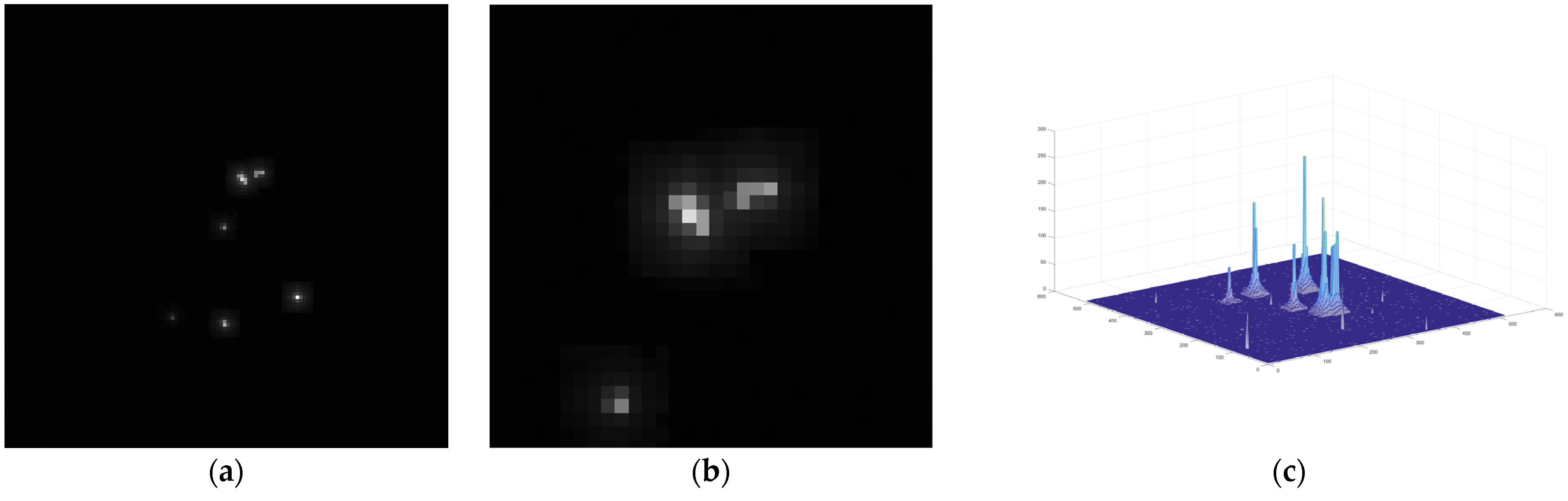
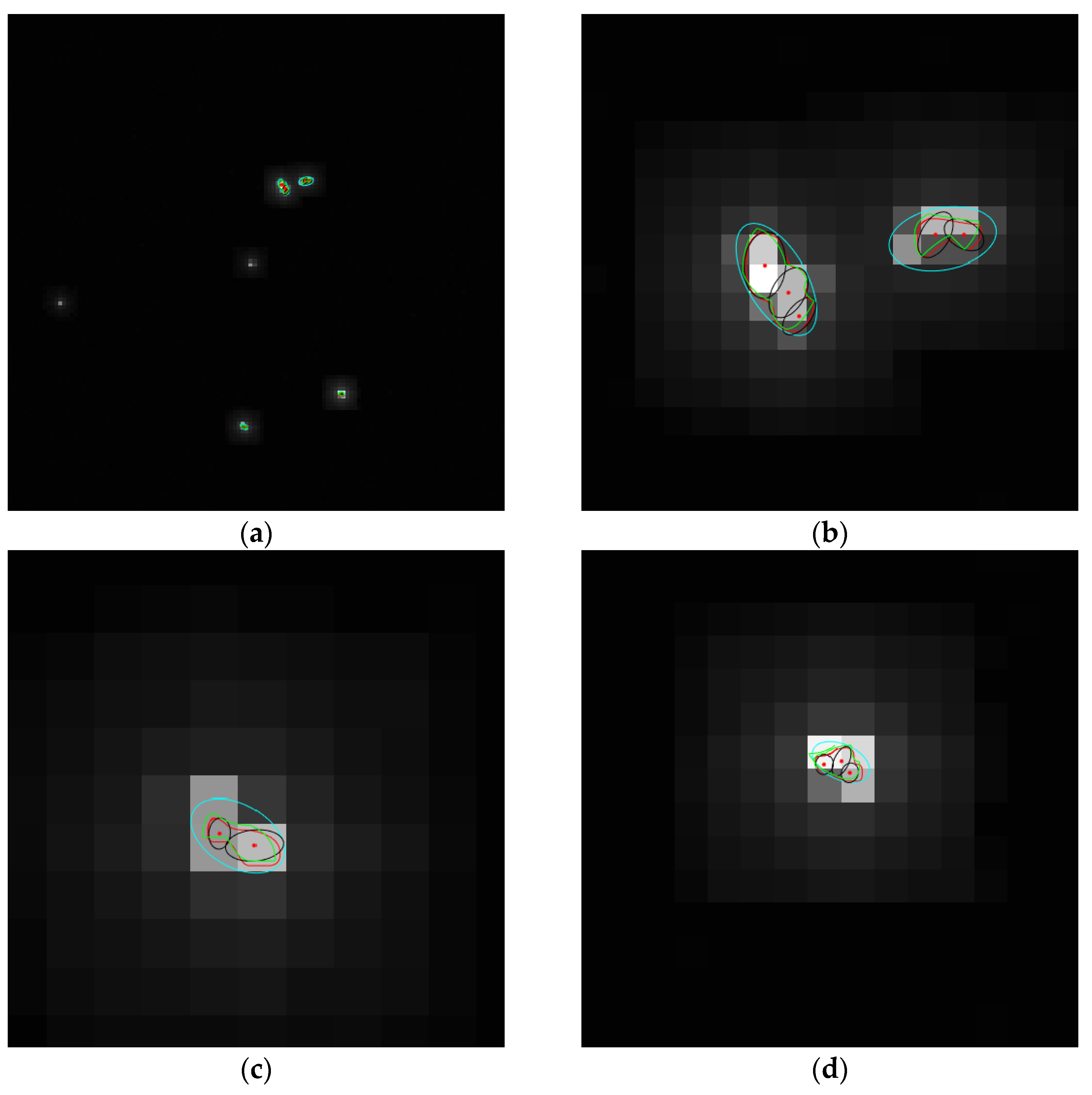
Extended targets are presented as multiple adjacent pixels in the infrared image plane with connectivity. Thus, the measurement partitioning of the infrared image can use the characteristics of connectivity and amplitude. As shown in Figure 2a, there are extended targets and clutter. Figure 2b is the enlarged local image which shows the details of the measurements. Figure 2c gives the amplitude of these clusters, which shows the difference between targets and clutter. Clearly, clutter occupies small areas and has a low amplitude. Thus, the extended target measurements can be obtained. In this study, all the measurements with an area smaller than are eliminated. Additionally, those with an amplitude less than are also eliminated. The partitioning steps are as follows.
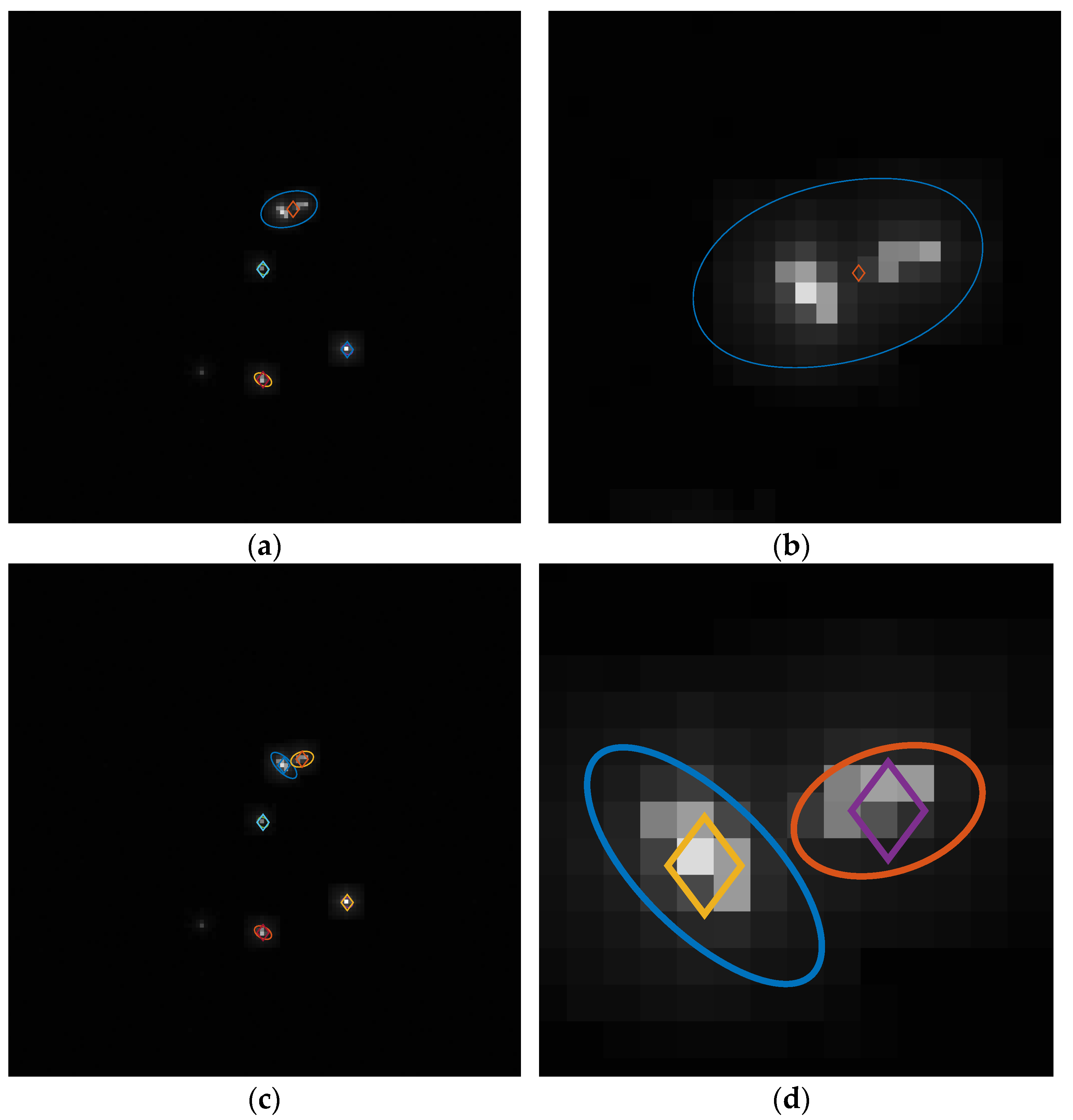
Step 1: The Hoshen–Kopelman (H-K) [28] algorithm is used to detect the connected regions in the image plane. The results are shown in Figure 3a,b. Figure 3a is the partitioning results of the 36th frame; Figure 3b is the enlarged image of two close extended targets which shows that the blue ellipse contains multiple local maxima, which can be further divided.
Step 2: Detect the local maxima in the clusters generated by H-K algorithm. As shown in Figure 2c, when the targets are close, the amplitude is superimposed, and wave peaks are formed. Thus, if there are multiple local maxima, each local maximum and its neighborhood contains at least one extended target.
Step 3: The clusters containing multiple local maxima are further partitioned using the k-means algorithm to produce new clusters. The results of partitioning are shown in Figure 3c,d. Figure 3c presents the partitioning results of frame 36 based on H-K with k-means; Figure 3d is an enlarged image of two close extended targets (H-K with k-means).
2.1.4. PMBM Filter for Extended Target
The recursion of the PMBM filter for the extended target is presented, which includes the prediction process and updated process. The PMBM RFS is given in the Ref. [5] for multiple extended targets and in the Ref. [27] for multiple point targets. According to these studies, the density is propagated by , .
- A.
- Prediction process
Given the posterior PMBM density at time is , and the dynamic model in Section 2.1.2, the predicted parameters at time can be expressed as
and the detailed proof process can be found in the Ref. [24].
- B.
- Updated process
Assuming that the predicted density is , , the measurement model and measurement set is given as Section 2.1.2, and the updated PMBM density is also in PMBM form.
where for the undetected targets,
and for the detected targets (including the first detected targets, the missed detected targets and the targets detected in all the steps),
where is the predicted likelihood, and denotes the measurement cell which corresponds to the data association . is the number of measurements in . represents the hypothesis weight. is the clutter intensity. is the space of all data associations for the th predicted MB. denotes non-empty cells, which contains measurements from a source (either clutter or a single target).
2.2. B-Spline
A B-spline is a piecewise polynomial function which can describe the shape of any curve by adjusting the location of the control points. More information on the B-spline can be found in the Refs. [29,30]. The B-spline curve with order can be described as
where is a control point, denotes the total number of control points and is the B-spline basis function, which is defined over a knot vector. The mathematical expression is as follows:
where the variables are knot elements.
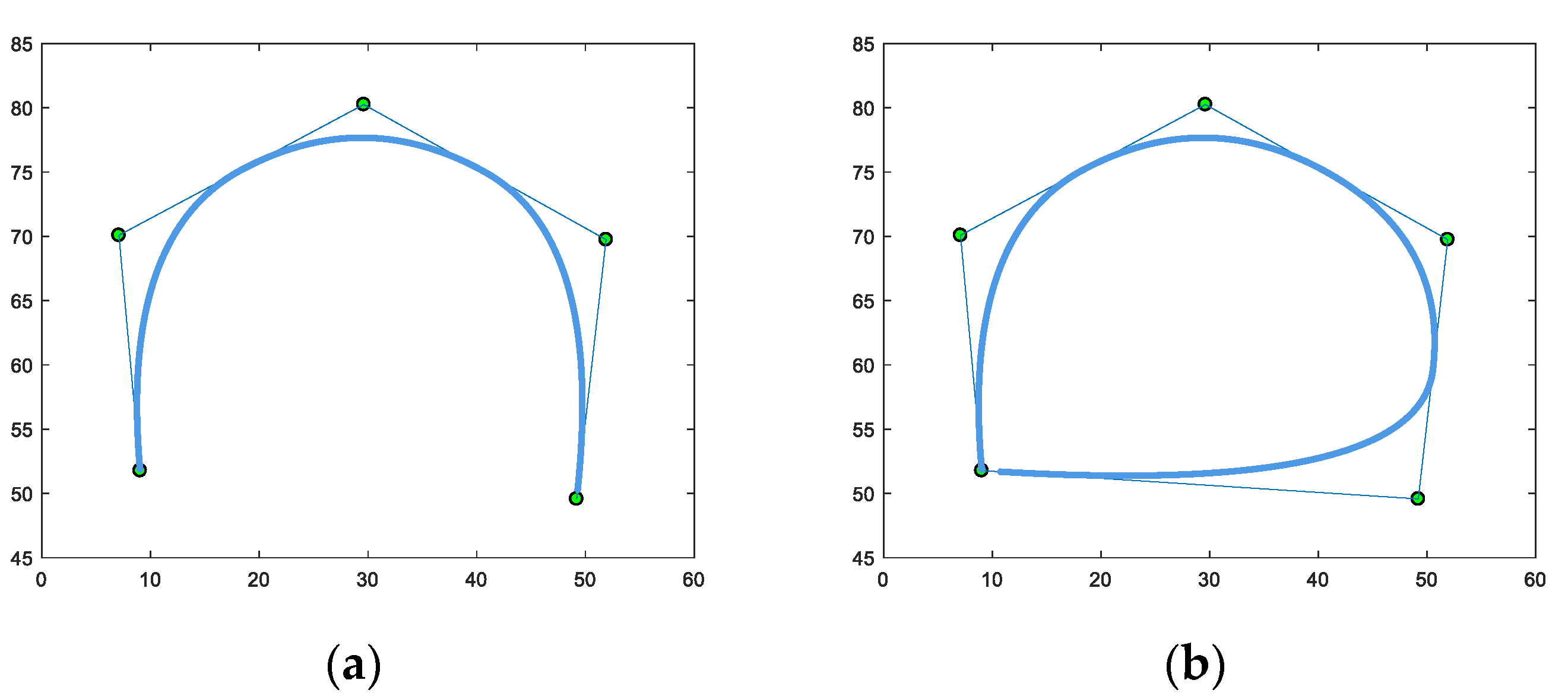
Generally, the B-spline curve is open, as Figure 4a shows, and a close curve can be obtained by repeating the first three control points, as Figure 4b shows. The B-spline used in this study is a closed curve, and the order is 3, that is, . The B-spline approach has been used in target tracking applications [16,17,31,32,33] in a continuous state space.
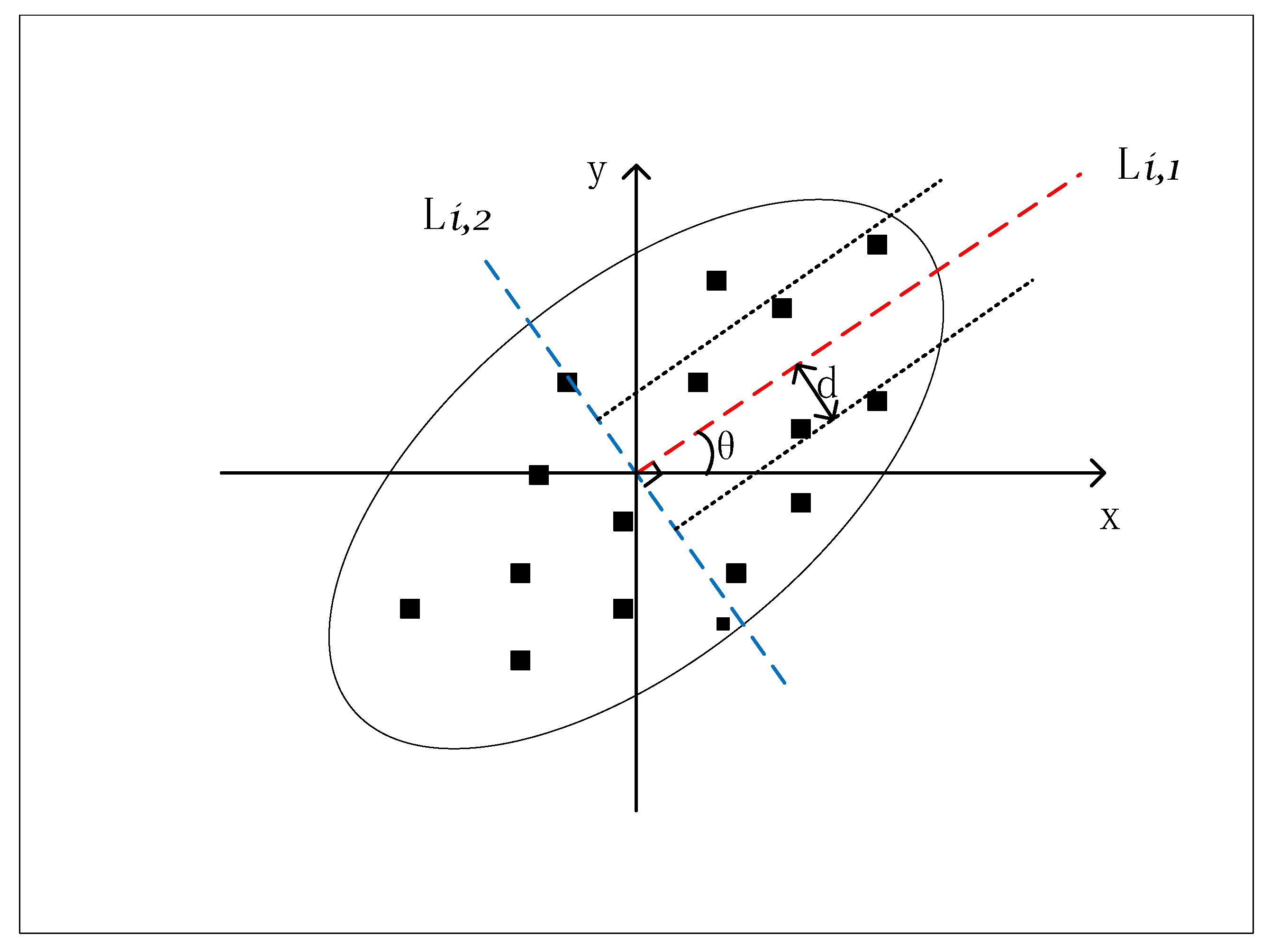
In this study, the control points are obtained as in the Ref. [16]. As shown in Figure 5 [34], suppose that is a pseudo-measurement set. More information on the construction of the pseudo-measurement set can be found in the Ref. [16]. The mean of is taken as the coordinates’ origin, and is divided into equal angles. Thus, the pseudo-measurement set can be divided by these angles. Let be the measurement set in the area of the th partition at time , which can be calculated by
where is the measurement in , and , denoting the position of the x- and y-coordinates at time . gives the width of a partition. (the red dotted line) is the line which goes through the origin of the coordinate and along the partition angle direction; it is defined as , where . (the blue dotted line) is the line which is perpendicular to line and also goes through the orign of the coordinate. is defined as , where .
Let and denote the polar radius and polar angles, respectively. can be obtained by
and thus, the matrix of control points can be expressed by , which can describe the shape of the targets. The matrix of control points is updated and predicted by implementing a one-dimensional Kalman filter. The specific equations can be found in the Ref. [16] (Equations (13)–(15)). The target shape can be estimated according to . First, convert the control points to Descartian coordinates, then fit the shape using a B-spline curve.
where is the control point positon in Descatian coordinates, and let . In addition, to obtain the closed curve, add three points , , , and make them equal to , and , respectively.
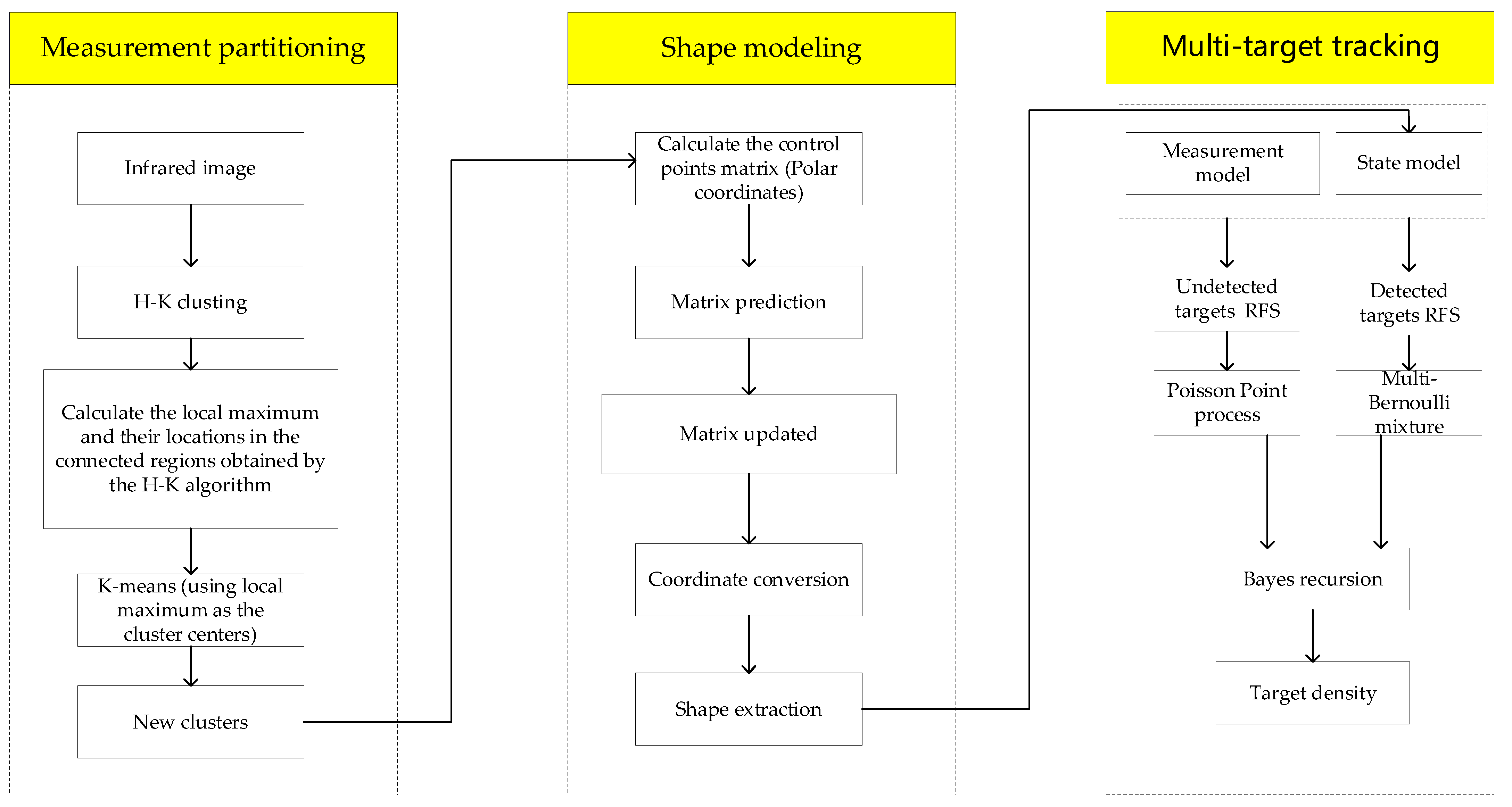
3. Proposed Algorithm
The proposed algorithm is presented in Figure 6, which can be divided into three steps: (1) amplitude-aided measurement partitioning; (2) shape modeling based on the control points of the B-spline; and (3) a multi-target tracking algorithm based on the PMBM filter. Step 1 can be implemented based on Section 2.1.3. Step 2 is performed in 2.2.
3.1. Single Extended Target
An extended target state at time is modeled as , where is the Poisson measurement rate parameter, is the kinematic state of the group center and denotes the shape state. As in the Ref. [5], the density of the rate parameter and kinematic state was modeled using the gamma distribution and Gaussian distribution, respectively. The shape state was modeled using a spatial probability distribution characterized by the control points of a B-spline. Thus, the target state distribution based on this model is a gamma-Gaussian-spline (GGS) and is denoted as
where and are parameters of gamma distribution, and denote the mean and covariance of Gaussian distribution, is the covariance of the shape and denotes control points.
3.2. GGS-PMBM Filter
The multiple extended target tracking algorithm is proposed based on the models presented above and the PMBM filter. The recursion is based on the following assumptions: (1) the survival probability is state-independent, that is, ; (2) the detection probability is state-independent, that is, ; and (3) the density of new targets at time is in GGS form.
The prediction process and updated process of the parameters of PPP components and Bernoulli components are given in the following:
Prediction step: Given the posterior GGS-PMBM density at time as , , , .
Undetected targets: Poisson rate of predicted PPP:
The predicted spatial distribution is
where the predicted parameters are computed as in Table 2. is the parameter of new targets. and are the Poisson rate of birth targets and undetected targets, respectively. and are the number of birth targets and undetected targets, respectively.
Detected targets: Prediction weights and number of components are unchanged. The probability of existence and spatial distribution are
where the parameters can be obtained using Table 2.
Updated step: Suppose that the predicted parameters are given as , , , .
The updated parameters for the detected targets and undetected targets are obtained using the following:
Undetected targets:
where is the probability that the target is not detected, and is defined as
The updated density is
where . There are two parts to the density. The first part corresponds to the detection process modeled using , which means missed detection. The second means that the Poisson random number of detections is zero.
Targets detected for the first time: A target is detected for the first time, and the set of detection is denoted by . The existence probability and spatial distribution can be expressed as
where
and are obtained using Table 1.
Targets detected in all steps: The Bernoulli component that exists all the time can be updated by a non-empty measurement set . The probability of existence is
and the spatial distribution can be expressed as
and are computed in Table 1.
Targets that missed detection: If the measurement set used to update the th Bernoulli in th MB components is empty, that is, , the existence probability is
where
The updated spatial distribution is
There are also two parts to this formula: the first part corresponds to the case in which the target is not detected, while the second part denotes that the target does not generate a measurement.
4. Results
To demonstrate the performance of the proposed algorithm, two long-wave infrared scenarios were simulated using a Satellite Tool Kit (STK) to demonstrate the performance of the proposed algorithm. The image size was 512 512 pixels, and there were 224 frames in total. The first scenario contains four targets, and there is no cross-trajectory. There are two targets in the second scenario. The details can be found in the following.
4.1. Scenario 1 (No-Crossing Track)
Figure 7 shows the real trajectories of the extended targets. All four extended targets appear in the first frame and disappear in frame 122, frame 138, frame 224 and frame 224. The target state , where , concludes the position and velocity. The initial state in which targets are born is listed in Table 3. The initial control points are defined as , where and . The sampling time is . The detection probability is , and the survival probability is . The transition matrix and the process noise covariance matrix are defined as:
where denotes the Kronecker product, . The proposed algorithm is compared to the approach based on RM and the approach based on multiple ellipses, which are denoted by GGIW-PMBM and Em-PMBM, respectively. In addition, the prior of the multiple ellipses, including the number, size and direction of the ellipses, needs to be given for the Em-PMBM-AP filter. The initial set of multiple ellipses is shown in Figure 8.
To demonstrate the effect of the measurement partition method on tracking performance, three methods are compared in this study: the amplitude-aided method (AP), the distance-based method (DP) and grid-based DBSCAN (GBDBSCAN) algorithm for which the density criterion was set to be a comparison of the mean amplitude in the search area to an amplitude threshold [23]. The modified optimal sub-pattern (mOSPA) [4,17] assignment metric was employed to assess the performance. If we suppose that the true state of an extended target is and the estimated state is , the mOSPA is defined as
where and are the true target state and the estimated target state, respectively, and
where , and were chosen to satisfy the maximum expected error for the measurement rate, kinematic state and extension state, respectively. is a radial function that maps an angle to the radius of an arbitrary shape from its centroid (from 0 to ; is the number of points that was evaluated at). The details can be found in the Ref. [17].
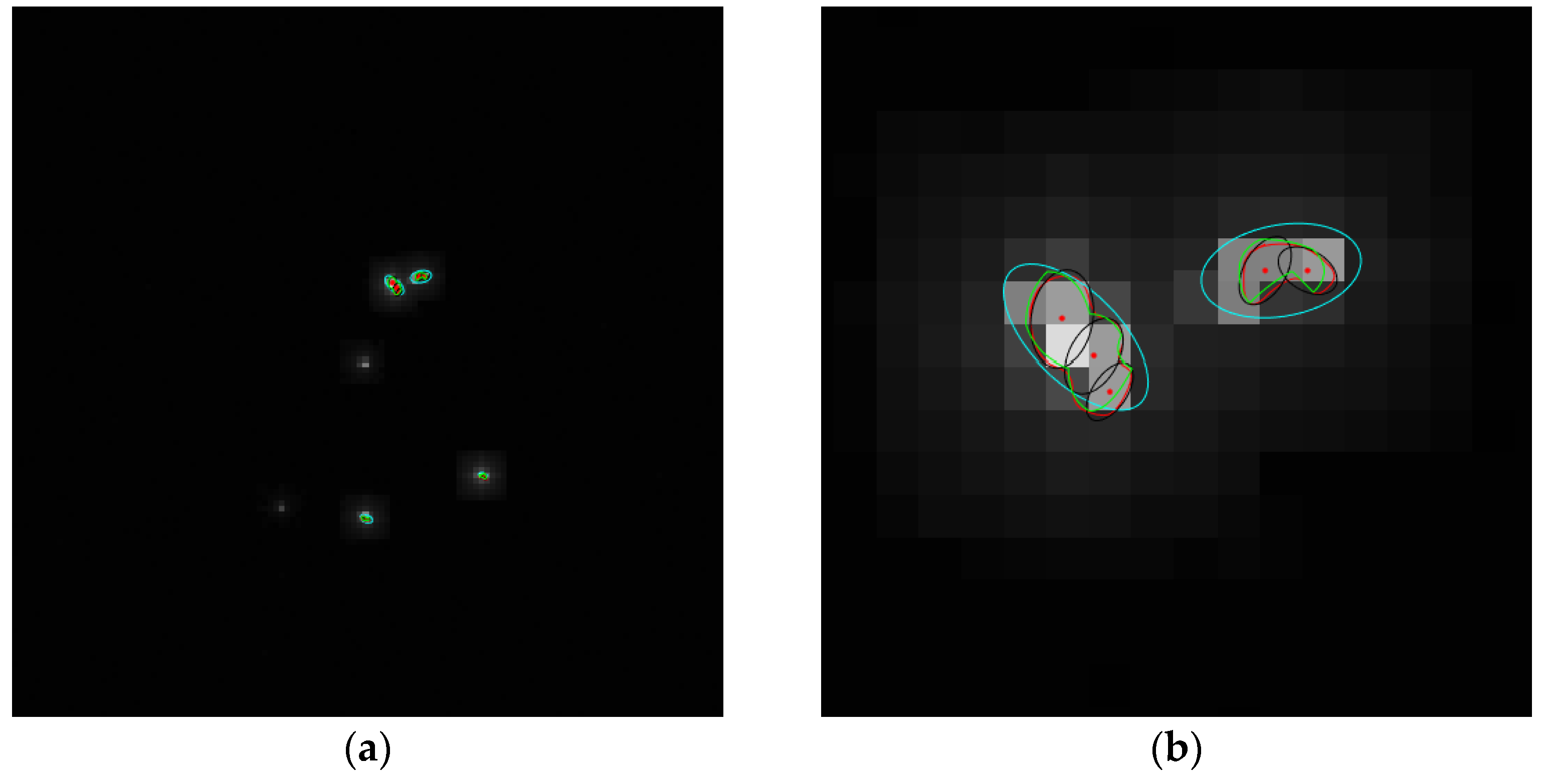
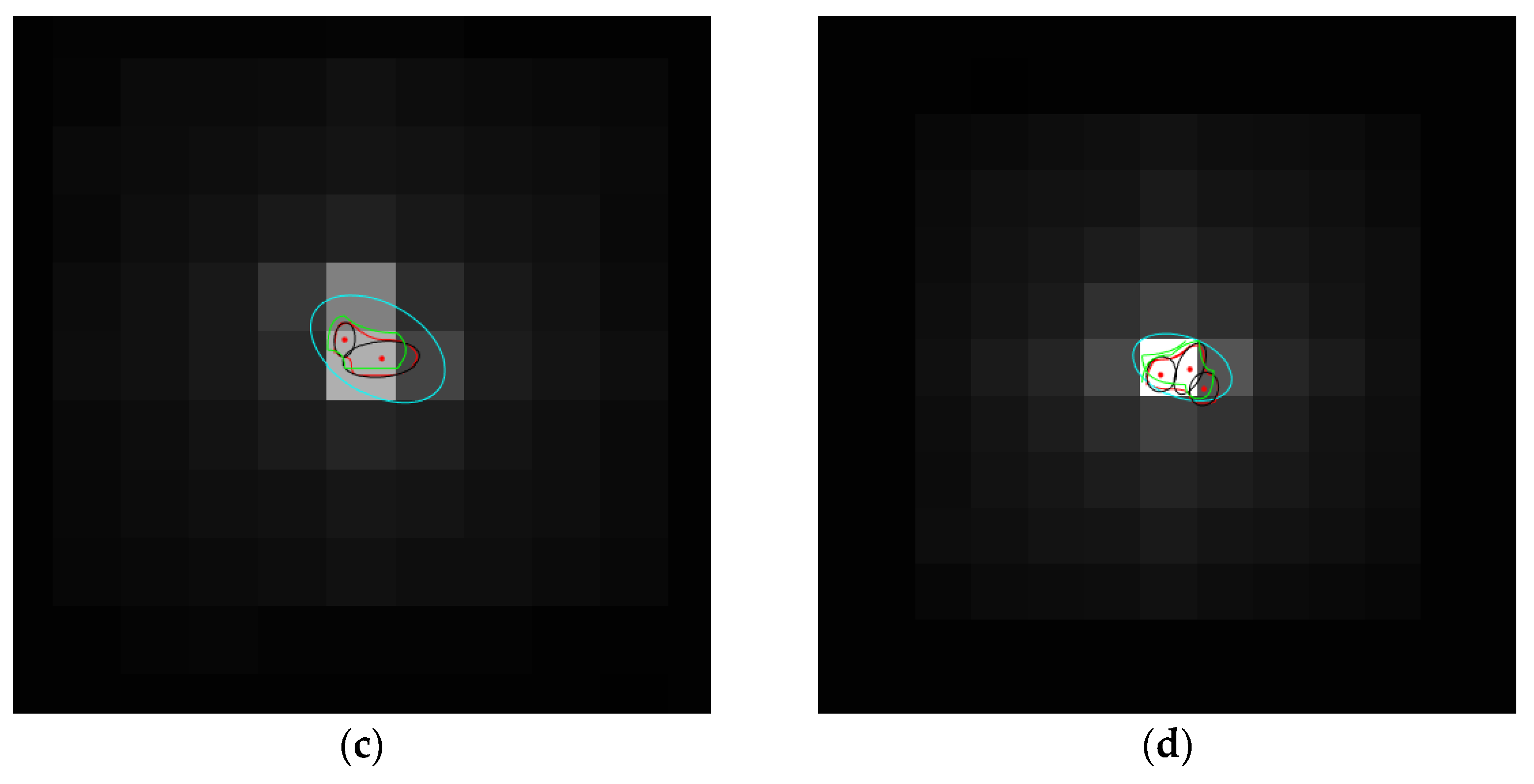
The effectiveness of the extension estimation of the proposed algorithm (GGS-PMBM-AP), the PMBM filter based on GGIW distribution with amplitude-aided partitioning (GGIW-PMBM-AP) and the PMBM filter based on multiple ellipses with amplitude-aided partitioning (Em-PMBM-AP) are demonstrated in Figure 9 and Figure 10, which present the images of frames 36 and 90, and have been plotted using green, blue and black lines, respectively. The truth shape is shown using a red line. It can be concluded from the results that the extension, shape and orientation of the targets can be estimated better by the GGS-PMBM-AP filter even if the shape changes. This is due to the application of the B-spline model, which can accurately fit the shape by changing the position of the control points.
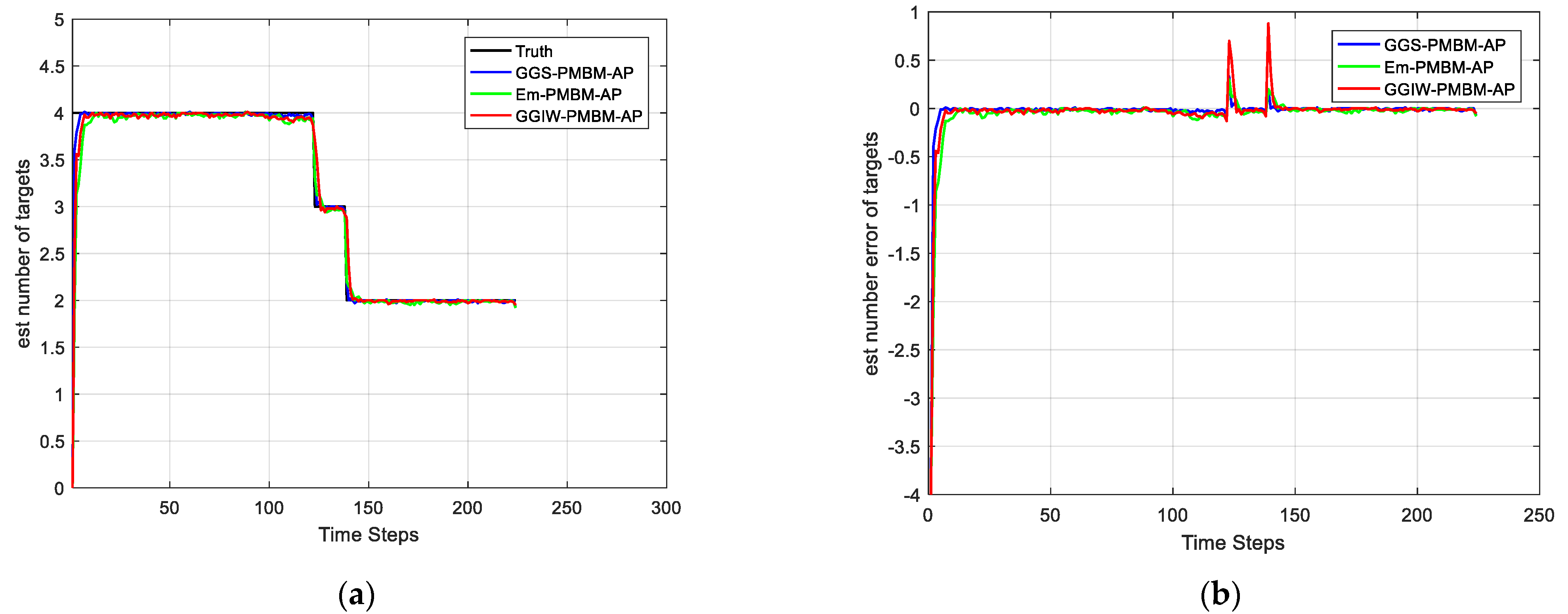
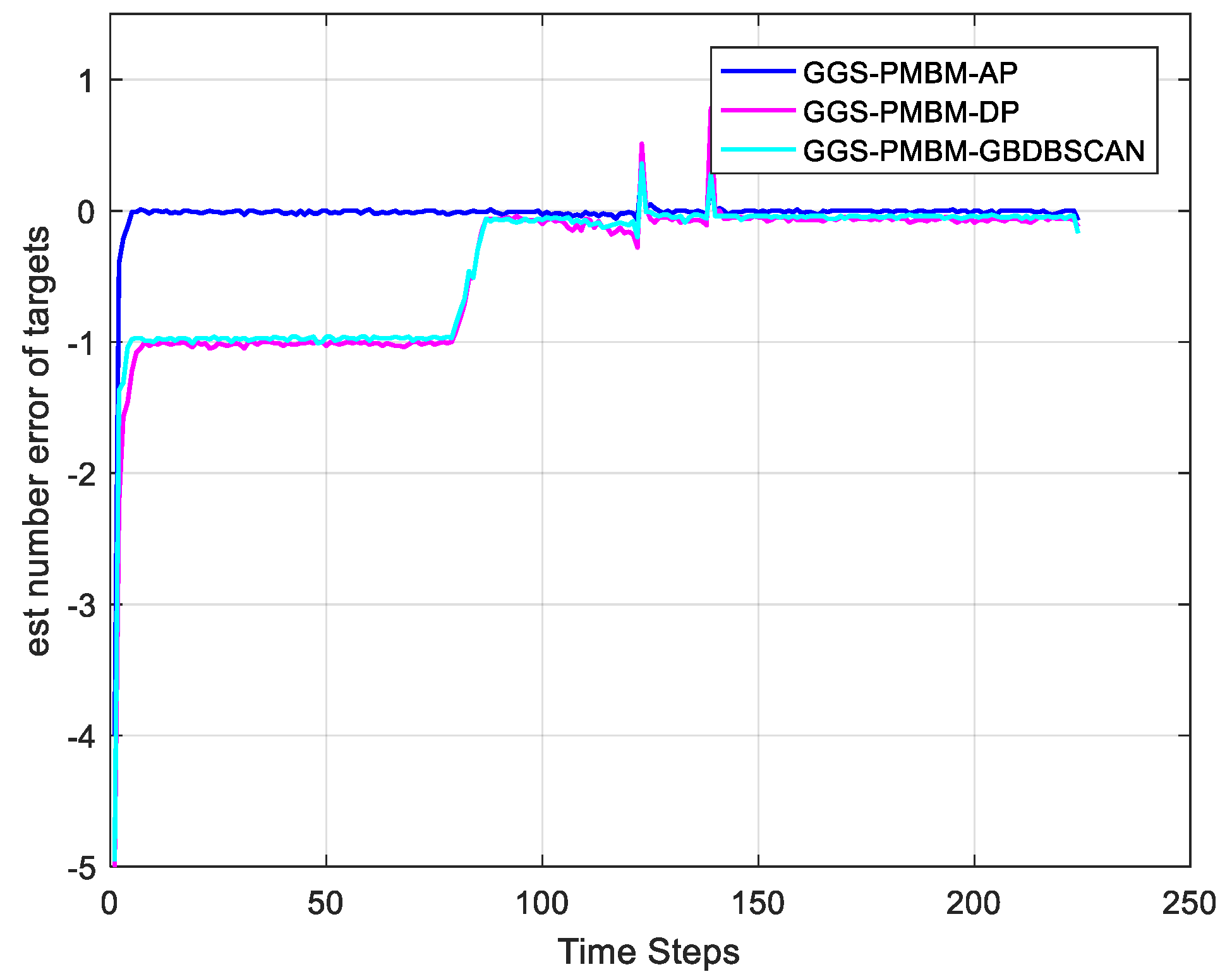
Figure 11 and Figure 12 show the averaged results over 100 Monte Carlo (MC) runs, corresponding to the performance metrics on mOSPA error and the number of targets. As can be seen in Figure 11a, the averaged mOSPA over 224 steps is 1.235572, 1.386461 and 1.425068 of the GGS-PMBM-AP filter, Em-PMBM-AP filter and GGIW-PMBM-AP filter, respectively. The GGS-PMBM-AP filter outperforms the Em-PMBM-AP filter and GGIW-PMBM-AP filter by 10% and 13%, respectively. This is due to the fact that the proposed B-spline model can more accurately estimate the extension even if the shape changes. Additionally, the Em-PMBM-AP filter offers better tracking accuracy than the GGIW-PMGM-AP filter due to its application of multiple ellipses. Figure 11b shows that the measurement partition method also has an impact on tracking accuracy, where the GGS-PMBM-AP filter outperforms the GGS-PMBM-DP filter and GGS-PMBM-GBDBSCAN filter. Since the amplitude threshold of the GBDBSCAN method is difficult to determine, the performance of the latter two methods is similar. Combining Figure 11b and Figure 13, it can be seen that the larger the number error, the worse the performance. Figure 12 shows the averaged number and number errors of all three filters. This error shows the difference between the estimated and true number of multiple extended targets. It can be seen that all filters are able to estimate the number of targets with minimal error.
The filters were run separately on an AMD Core 3.20 GHz CPU PC with 16 GB RAM and MATLAB R2021b. The computational complexity is illustrated by comparing the cost time. Based on 100 Monte Carlo runs, the average computational times of the filters are shown in Table 4. It can be seen that the computational complexity of GGS-PMBM-DP is slightly higher than the GGS-PMBM-AP filter, proving that the amplitude-aided measurement portioning method is more effective than the method based on distance. The GGS-PMBM-GBDBSCAN algorithm has the smallest running time, which is due to the faster running speed of the clustering algorithm. In addition, the GGS-PMBM-AP filter takes more time to tackle the multiple control points. Thus, the complexity of the GGS-PMBM-AP filter is the highest.
4.2. Scenario 2 (Crossing Tracks)
There are two extended targets, the trajectories of which are shown in Figure 14. In this scenario, tracks cross at step 102. The initial state is as in Table 5. Other parameters are the same as Scenario 1. The target shape is simulated as in Figure 8b.
Figure 15 shows the averaged mOSPA over 100 MC runs. There is a peak when the tracks cross. The difference in performance remains consistent with Scenario 1, thus demonstrating the effectiveness of the proposed algorithm.
5. Discussion
An amplitude-aided PMBM filter based on B-spline has been proposed for tracking multiple extended targets. As observed in Section 4, it can be concluded that the proposed algorithm can estimate the shape of targets more accurately compared to the other two methods. This is mainly because the control points can be adjusted in real time according to the estimated parameters, which will help to fit the real shape.
In addition, although the original intention was to estimate the shape of the target more accurately, the proposed algorithm shows better performance on the kinematic state. This can be attributed to the inherent coupling relationship between shape and motion. Because the target is captured accurately, there is an obvious improvement in the estimation performance of the kinematic state. Conversely, an accurate estimation of the target position will help to describe the shape of the target. This also explains why an accurate estimation of the shape can also improve the performance of the kinematic state. Meanwhile, the introduction of the amplitude information further contributes to the improvement of performance due to the accurate partitioning of measurement data.
6. Conclusions
A new tracking algorithm of multiple infrared non-ellipsoidal extended targets, namely GGS-PMBM, was proposed in this study to estimate the shape of the extended target. This algorithm utilizes the PMBM framework in order to implement the tracking of multiple targets. For the state of the extended target, a B-spline was employed to fit the shape by iterating control points. In addition, the measurement partition was also improved using the infrared image characteristic. Specifically, the local maximum of amplitudes in the connected domain was used as the clustering center, and clustering was performed. To verify the algorithm, a scenario using STK was simulated, and a series of infrared images were obtained. The two different scenario simulation results showed that the proposed algorithm can accurately estimate the shape of targets, and outperformed the Em-PMBM filter and the GGIW-PMBM filter. This algorithm can also be applied to group target tracking with slight modifications. In future work, it would be worthwhile to verify these findings using real data. In addition, the splitting and merging of group targets and track management issues were not addressed in this study, which are of great importance in practical scenarios.
Author Contributions
Y.W. conceived of the idea, performed the simulation and wrote the paper; X.C. simulated the infrared image, helped edit and offered some useful suggestions with regard to methodology with P.R. C.G. mainly simulated the infrared scenario and checked the paper. All authors have read and agreed to the published version of the manuscript.
Funding
This research was funded by the National Natural Science Foundation of China (No. 62175251).
Data Availability Statement
Not applicable.
Conflicts of Interest
The authors declare no conflict of interest.
References
- Vo, B.-N.; Mallick, M.; Bar-Shalom, Y.; Coraluppi, S.; Osborne, R.; Mahler, R.; Vo, B.-T. Multitarget tracking. Wiley Encycl. Electr. Electron. Eng. 2015, 2015. [Google Scholar]
- Bouraya, S.; Belangour, A. Multi object tracking: A survey. In Proceedings of the Thirteenth International Conference on Digital Image Processing (ICDIP 2021), Singapore, 20–23 May 2021; pp. 142–152. [Google Scholar]
- Granstrom, K.; Baum, M.; Reuter, S. Extended object tracking: Introduction, overview and applications. arXiv 2016, arXiv:00970. [Google Scholar]
- Liang, Z.; Liu, F.; Li, L.; Gao, J. Improved generalized labeled multi-Bernoulli filter for non-ellipsoidal extended targets or group targets tracking based on random sub-matrices. Digit. Signal Process. 2020, 99, 102669. [Google Scholar] [CrossRef]
- Granström, K.; Fatemi, M.; Svensson, L. Poisson multi-Bernoulli mixture conjugate prior for multiple extended target filtering. IEEE Trans. Aerosp. Electron. Syst. 2019, 56, 208–225. [Google Scholar] [CrossRef] [Green Version]
- Granström, K.; Lundquist, C.; Orguner, U. Tracking rectangular and elliptical extended targets using laser measurements. In Proceedings of the 14th International Conference on Information Fusion, Chicago, IL, USA, 5–8 July 2011; pp. 1–8. [Google Scholar]
- Gilholm, K.; Salmond, D.J.I.P.-R. Sonar, Navigation, Spatial distribution model for tracking extended objects. IEE Proc. Radar Sonar Navig. 2005, 152, 364–371. [Google Scholar] [CrossRef]
- Koch, J.W. Bayesian approach to extended object and cluster tracking using random matrices. IEEE Trans. Aerosp. Electron. Syst. 2008, 44, 1042–1059. [Google Scholar] [CrossRef]
- Granström, K.; Natale, A.; Braca, P.; Ludeno, G.; Serafino, F. Gamma Gaussian inverse Wishart probability hypothesis density for extended target tracking using X-band marine radar data. IEEE Trans. Geosci. Remote Sens. 2015, 53, 6617–6631. [Google Scholar] [CrossRef]
- García-Fernández, Á.F.; Williams, J.L.; Svensson, L.; Xia, Y. A Poisson multi-Bernoulli mixture filter for coexisting point and extended targets. IEEE Trans. Signal Process. 2021, 69, 2600–2610. [Google Scholar] [CrossRef]
- Beard, M.; Reuter, S.; Granström, K.; Vo, B.-T.; Vo, B.-N.; Scheel, A. Multiple extended target tracking with labeled random finite sets. IEEE Trans. Signal Process. 2015, 64, 1638–1653. [Google Scholar] [CrossRef] [Green Version]
- Lan, J.; Li, X.R. Tracking of maneuvering non-ellipsoidal extended object or target group using random matrix. IEEE Trans. Signal Process. 2014, 62, 2450–2463. [Google Scholar] [CrossRef]
- Baum, M.; Hanebeck, U.D. Extended object tracking with random hypersurface models. IEEE Trans. Aerosp. Electron. Syst. 2014, 50, 149–159. [Google Scholar] [CrossRef] [Green Version]
- Cao, X.; Lan, J.; Li, X.R. Extension-deformation approach to extended object tracking. IEEE Trans. Aerosp. Electron. Syst. 2020, 57, 866–881. [Google Scholar] [CrossRef]
- Han, Y.; Xu, H.; Hu, G.; Han, C. An Extended Target Tracking Algorithm Based on Gaussian Surface Fitting. Math. Probl. Eng. 2022, 2022. [Google Scholar] [CrossRef]
- Yang, J.-L.; Li, P.; Ge, H.-W. Extended target shape estimation by fitting B-spline curve. J. Appl. Math. 2014, 2014, 1–9. [Google Scholar] [CrossRef] [Green Version]
- Daniyan, A.; Lambotharan, S.; Deligiannis, A.; Gong, Y.; Chen, W.-H. Bayesian multiple extended target tracking using labeled random finite sets and splines. IEEE Trans. Signal Process. 2018, 66, 6076–6091. [Google Scholar] [CrossRef] [Green Version]
- Naujoks, B.; Burger, P.; Wuensche, H.-J. Fast 3D extended target tracking using NURBS surfaces. In Proceedings of the IEEE Intelligent Transportation Systems Conference (ITSC), Auckland, New Zealand, 27–30 October 2019; pp. 1104–1109. [Google Scholar]
- Yang, K.; Zhong, C.; Zhang, X.; Zhu, X.; Yue, Y. 3D modeling of riverbeds based on NURBS algorithm. In Proceedings of the 2020 3rd International Conference on Artificial Intelligence and Pattern Recognition, Xiamen, China, 26–28 June 2020; pp. 163–167. [Google Scholar]
- Piegl, L.J.I.C.G. Applications, on NURBS: A survey. IEEE Comput. Graph. 1991, 11, 55–71. [Google Scholar] [CrossRef]
- Granstrom, K.; Orguner, U. A PHD filter for tracking multiple extended targets using random matrices. IEEE Trans. Signal Process. 2012, 60, 5657–5671. [Google Scholar] [CrossRef] [Green Version]
- Li, Y.; Xiao, H.; Song, Z.; Hu, R.; Fan, H. A new multiple extended target tracking algorithm using PHD filter. Signal Process. 2013, 93, 3578–3588. [Google Scholar] [CrossRef]
- Kellner, D.; Klappstein, J.; Dietmayer, K. Grid-based DBSCAN for clustering extended objects in radar data. In Proceedings of the IEEE Intelligent Vehicles Symposium, Madrid, Spain, 3–7 June 2012; pp. 365–370. [Google Scholar]
- Williams, J.L. Marginal multi-Bernoulli filters: RFS derivation of MHT, JIPDA, and association-based MeMBer. IEEE Trans. Aerosp. Syst. 2015, 51, 1664–1687. [Google Scholar] [CrossRef] [Green Version]
- Vo, B.-T.; Vo, B.-N. Labeled random finite sets and multi-object conjugate priors. IEEE Trans. Signal Process. 2013, 61, 3460–3475. [Google Scholar] [CrossRef]
- Xia, Y.; Granstrcom, K.; Svensson, L.; García-Fernández, Á.F. Performance evaluation of multi-bernoulli conjugate priors for multi-target filtering. In Proceedings of the 20th International Conference on Information Fusion (Fusion), Xi’an, China, 10–13 June 2017; pp. 1–8. [Google Scholar]
- García-Fernández, Á.F.; Williams, J.L.; Granström, K.; Svensson, L. Poisson multi-Bernoulli mixture filter: Direct derivation and implementation. IEEE Trans. Aerosp. Electron. Syst. 2018, 54, 1883–1901. [Google Scholar] [CrossRef] [Green Version]
- Hoshen, J.; Kopelman, R. Percolation and cluster distribution. I. Cluster multiple labeling technique and critical concentration algorithm. Phys. Rev. B 1976, 14, 3438. [Google Scholar] [CrossRef]
- De Boor, C.; De Boor, C. A Practical Guide to Splines; Springer: New York, NY, USA, 1978; Volume 27. [Google Scholar]
- De Boor, C. Corrections and Emendations for a Practical Guide to Splines. Available online: https://pages.cs.wisc.edu/~deboor/pgs_errata.pdf (accessed on 16 November 2022).
- He, X.; Sithiravel, R.; Tharmarasa, R.; Balaji, B.; Kirubarajan, T. A spline filter for multidimensional nonlinear state estimation. Signal Process. 2014, 102, 282–295. [Google Scholar] [CrossRef]
- Sithiravel, R.; McDonald, M.; Balaji, B.; Kirubarajan, T. Multiple model spline probability hypothesis density filter. IEEE Trans. Aerosp. Electron. Syst. 2016, 52, 1210–1226. [Google Scholar] [CrossRef]
- Sithiravel, R.; Chen, X.; Tharmarasa, R.; Balaji, B.; Kirubarajan, T. The spline probability hypothesis density filter. IEEE Trans. Signal Process. 2013, 61, 6188–6203. [Google Scholar] [CrossRef]
- Li, P.; Ge, H.-W.; Yang, J.-L.; Wang, W.J.S.P. Modified Gaussian inverse Wishart PHD filter for tracking multiple non-ellipsoidal extended targets. Signal Process. 2018, 150, 191–203. [Google Scholar] [CrossRef]
- Granström, K.; Orguner, U. On the reduction of gaussian inverse wishart mixtures. In Proceedings of the 15th International Conference on Information Fusion, Singapore, 9–12 July 2012; pp. 2162–2169. [Google Scholar]
- Granström, K.; Orguner, U. Estimation and maintenance of measurement rates for multiple extended target tracking. In Proceedings of the 2012 15th International Conference on Information Fusion, Singapore, 9–12 July 2012; pp. 2170–2176. [Google Scholar]
Figure 1.
The partitioning results, corresponding to three different distance thresholds. (a) the original image (partition distance/pixel: 2.5); (b) the enlarged image of (a); (c) the original image (partition distance/pixel: 4.5); (d) the enlarged image of (c); (e) the original image (partition distance/pixel: 8.2); (f) the enlarged image of (e).

Figure 2.
(a) Infrared image of extended targets; (b) Enlarged image of two close extended targets; (c) The amplitude of targets and clutter.
Figure 2.
(a) Infrared image of extended targets; (b) Enlarged image of two close extended targets; (c) The amplitude of targets and clutter.

Figure 3.
Results of measurement partitioning based on the amplitude of the infrared image. (a) the partitioning result of the frame 36th using H-K algorithm; (b) the enlarged image of (a); (c) the further divided result using k-means; (d) the enlarged image of (c).
Figure 3.
Results of measurement partitioning based on the amplitude of the infrared image. (a) the partitioning result of the frame 36th using H-K algorithm; (b) the enlarged image of (a); (c) the further divided result using k-means; (d) the enlarged image of (c).

Figure 4.
This is a representation of B-spline: (a) open spline; (b) closed spline.

Figure 5.
Calculation of the control points. Squares are the measurements.

Figure 6.
The pipeline of the proposed algorithm.

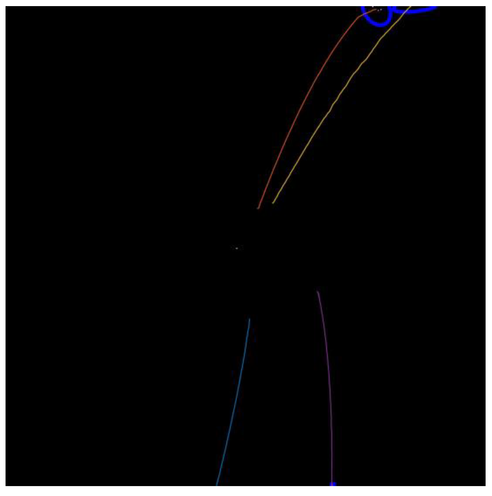
Figure 7.
True trajectories of the targets. The orange line denotes the trajectory of the first target. The yellow line denotes the trajectory of the second target. The blue line denotes the trajectory of the third target. The purple line denotes the trajectory of the fourth target.
Figure 7.
True trajectories of the targets. The orange line denotes the trajectory of the first target. The yellow line denotes the trajectory of the second target. The blue line denotes the trajectory of the third target. The purple line denotes the trajectory of the fourth target.

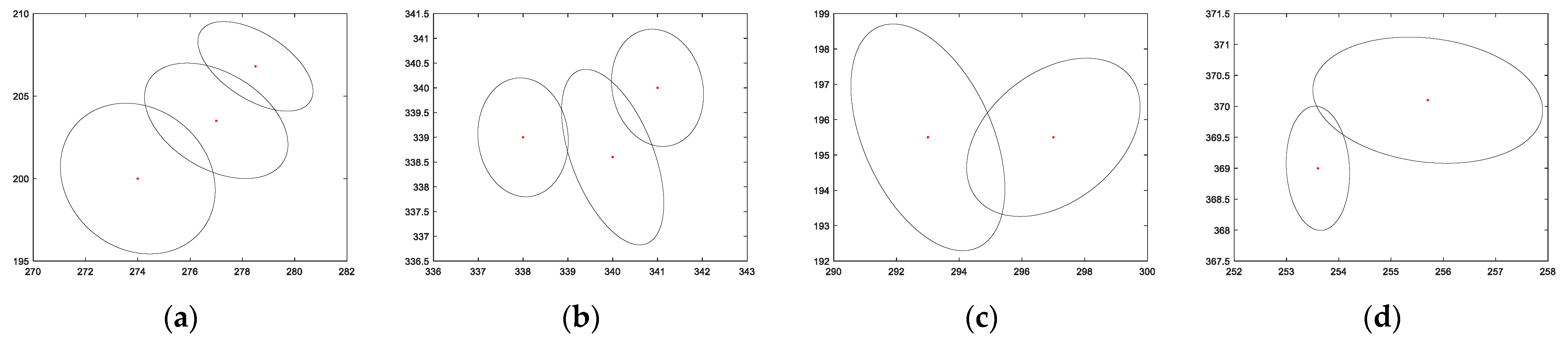
Figure 8.
Initial set for multiple ellipses method. (a–d) are four different models of shapes.

Figure 9.
The extension estimation of extended targets under different algorithms for frame 36. (a) estimation of extension; (b) enlarged image of target 1 and target 2; (c) enlarged image of target 3; (d) enlarged image of target 4.
Figure 9.
The extension estimation of extended targets under different algorithms for frame 36. (a) estimation of extension; (b) enlarged image of target 1 and target 2; (c) enlarged image of target 3; (d) enlarged image of target 4.


Figure 10.
The extension estimation of extended targets under different algorithms for frame 90. (a) the estimation of extension; (b) enlarged image of target 1 and target 2; (c) enlarged image of target 3; (d) enlarged image of target 4.
Figure 10.
The extension estimation of extended targets under different algorithms for frame 90. (a) the estimation of extension; (b) enlarged image of target 1 and target 2; (c) enlarged image of target 3; (d) enlarged image of target 4.

Figure 11.
Averaged mOSPA. (a) the performance of different tracking algorithm based on the same measurement partition method; (b) the performance of different measurement partition methods based on the same tracking algorithm.
Figure 11.
Averaged mOSPA. (a) the performance of different tracking algorithm based on the same measurement partition method; (b) the performance of different measurement partition methods based on the same tracking algorithm.

Figure 12.
Averaged cardinality and cardinality error of the GGS-PMBM-AP filter, Em-PMBM-AP filter and GGIW-PMBM-AP filter over 100 Monte Carlo runs. (a) Estimated number of targets, (b) cardinality error of targets estimation.
Figure 12.
Averaged cardinality and cardinality error of the GGS-PMBM-AP filter, Em-PMBM-AP filter and GGIW-PMBM-AP filter over 100 Monte Carlo runs. (a) Estimated number of targets, (b) cardinality error of targets estimation.

Figure 13.
Averaged cardinality error of the GGS−PMBM−AP filter, GGS−PMBM−DP filter and GGS−PMBM−GBDBSCAN over 100 Monte Carlo runs.
Figure 13.
Averaged cardinality error of the GGS−PMBM−AP filter, GGS−PMBM−DP filter and GGS−PMBM−GBDBSCAN over 100 Monte Carlo runs.

Figure 14.
The trajectories of two targets. The bule line is the trajectory of the first target. The red line is the trajectory of the second target.
Figure 14.
The trajectories of two targets. The bule line is the trajectory of the first target. The red line is the trajectory of the second target.

Figure 15.
Averaged cardinality and cardinality error of GGS−PMBM−AP filter, Em−PMBM−AP filter and GGIW−PMBM−AP filter over 100 Monte Carlo runs. (a) Estimated number of targets, (b) cardinality error of targets estimation.
Figure 15.
Averaged cardinality and cardinality error of GGS−PMBM−AP filter, Em−PMBM−AP filter and GGIW−PMBM−AP filter over 100 Monte Carlo runs. (a) Estimated number of targets, (b) cardinality error of targets estimation.


Table 1.
Updated GGS parameters of a single extended target.
| Input and set of detection |
| where |
| Likelihood: |
| Output: and likelihood |
Table 2.
Predicted GGS parameters of a single extended target.
| Input: |
| Output: |
where is the transition matrix and is the process noise.
Table 3.
The initial states of the targets.
| Target | State | Survival Time (Frame) |
|---|---|---|
| 1 | ||
| 2 | ||
| 3 | ||
| 4 |
Table 4.
Average computational times.
| Filter | GGS-PMBM-AP | Em-PMBM-AP | GGIW-PMBM-AP | GGS-PMBM-DP | GGS-PMBM-GBDBSCAN |
|---|---|---|---|---|---|
| Time | 10.07 s | 9.95 s | 9.91 s | 10.34 s | 9.57s |
Table 5.
The initial states of targets.
| Target | State | Survival Time (Frame) |
|---|---|---|
| 1 | ||
| 2 |
Disclaimer/Publisher’s Note: The statements, opinions and data contained in all publications are solely those of the individual author(s) and contributor(s) and not of MDPI and/or the editor(s). MDPI and/or the editor(s) disclaim responsibility for any injury to people or property resulting from any ideas, methods, instructions or products referred to in the content. |
© 2023 by the authors. Licensee MDPI, Basel, Switzerland. This article is an open access article distributed under the terms and conditions of the Creative Commons Attribution (CC BY) license (https://creativecommons.org/licenses/by/4.0/).
Share and Cite
MDPI and ACS Style
Wang, Y.; Chen, X.; Gong, C.; Rao, P. Non-Ellipsoidal Infrared Group/Extended Target Tracking Based on Poisson Multi-Bernoulli Mixture Filter and B-Spline. Remote Sens. 2023, 15, 606. https://doi.org/10.3390/rs15030606
AMA Style
Wang Y, Chen X, Gong C, Rao P. Non-Ellipsoidal Infrared Group/Extended Target Tracking Based on Poisson Multi-Bernoulli Mixture Filter and B-Spline. Remote Sensing. 2023; 15(3):606. https://doi.org/10.3390/rs15030606
Chicago/Turabian StyleWang, Yi, Xin Chen, Chao Gong, and Peng Rao. 2023. "Non-Ellipsoidal Infrared Group/Extended Target Tracking Based on Poisson Multi-Bernoulli Mixture Filter and B-Spline" Remote Sensing 15, no. 3: 606. https://doi.org/10.3390/rs15030606
Note that from the first issue of 2016, this journal uses article numbers instead of page numbers. See further details here.