1. Introduction
Remote sensing image scene classification has various applications in a wide range of scenarios, including environment monitoring, urban planning, spatial-temporal data analysis and smart cities. Owing to the development of image equipment for earth observation [
1,
2,
3], remote sensing images with different resolutions are increasing daily, which boosts the demand for intelligent interpretation of land use and land cover scenes.
Remote sensing image scene classification is a popular research field in satellite image analysis. During the past decades, numerous effective methods have emerged to achieve continuous improvement. Earlier methods, such as bag-of-visual words (BoVW) [
4], HOG [
5] and SIFT [
6], generally require rigorous design from experts to extract valuable features, which imposes certain limitations on feature extraction. More recently, algorithms based on deep learning have achieved satisfactory results in many application fields owing to their strong feature representation power and powerful graphical processing units. Among the deep learning methods, convolutional neural networks (CNNs) have been successfully applied in remote sensing image scene classification [
7,
8,
9,
10,
11,
12,
13,
14]. Compared with traditional unsupervised feature learning methods, feature representations with more complex patterns can be learned via deep architecture neural networks. Some extensively used pre-trained networks, such as AlexNet [
15] and VGG-VD [
16], have been proved to achieve excellent performance on remote sensing image scene classification [
17].
However, CNNs are considered as a black-box operation mechanism, which means humans cannot easily understand the decision-making process. Therefore, the explainability of the model, which is considered as a barrier to developing artificial intelligence, has attracted increasing attention. When exploiting a machine learning model, considering the interpretability of the system can lead to the correction of model deficiencies and also improve implementability. For example, the improvement of explainability can help ensures overall impartiality in many applications involving ethics. To address this issue, many attempts have been made from various aspects [
18,
19,
20,
21,
22,
23,
24,
25,
26,
27]. A deep generator network (DGN), which generates the most representative image for a given output neuron, was proposed in [
18]. The authors in [
20] used a different approach called network dissection to quantify the interpretability of the latent representations of CNNs. In the field of remote sensing, long short-term memory (LSTM) recurrent neural networks were used by the authors in [
26] to discover the interpretability of crop yield estimation. A synthetic aperture radar (SAR) specific deep learning framework called Deep SAR-Net that considers complex-valued SAR images to learn both spatial texture information and backscattering patterns of objects, was proposed in [
27].
Compared with the aforementioned explainability techniques, local explanation methods which provide a visual saliency map for each specific decision are more widely studied. The saliency map, where the relevance score of each spatial position indicates its contribution to the prediction, is generally presented as a heat map. Consequently, it is more intuitive and comprehensible. One of the seminal works in this category was [
19]. The authors of [
19] utilized a global average pooling layer to modify and substitute the fully-connected layers. A class activation map (CAM) that highlights the image regions that are relatively important for a specific object class was achieved by projecting back the weights of the output layer on the convolutional feature maps. However, the CAM alters models’ architectures, making it difficult to apply to a wide variety of CNN model families. Later, authors [
28] proposed a gradient-weighted class activation mapping (Grad-CAM), which uses the gradients of any target concept, flowing into the final convolutional layer, to produce a coarse localization map. This approach avoids modifying the models’ architectures.
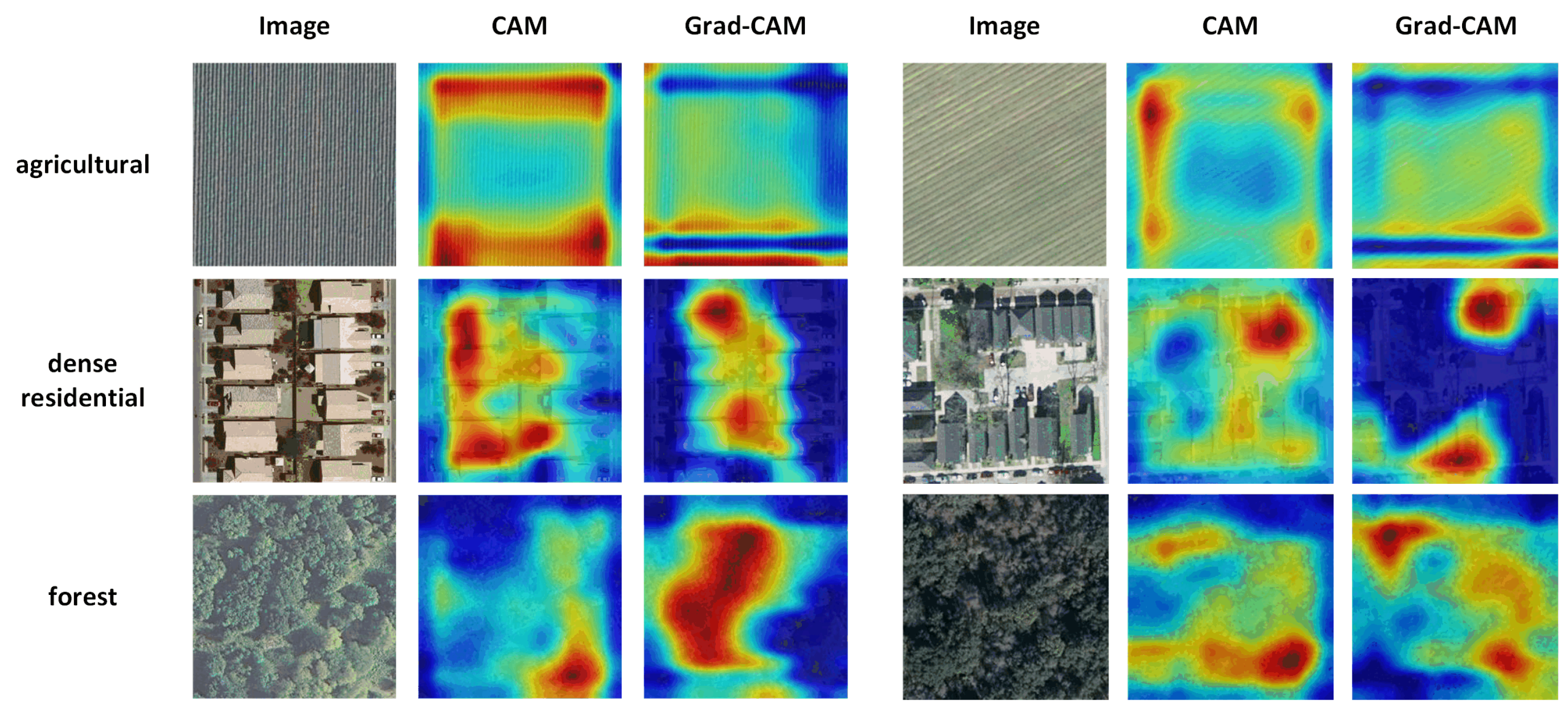
Existing visual explanation methods, such as those mentioned above, have the identical feature that they almost solely pay attention to the saliency map of the final convolutional layer of CNNs. Some of these algorithms cannot visualize middle or shallow layers owing to the change of the original model, such as CAM. The feature maps of the final layer draw more attention, mainly because the receptive field of the high layer is larger than that of the shallow layer, which means the saliency map obtained by the high layer may contain more whole objects or object parts and may be more visually comprehensive. Besides, most visual explanation research is carried out based on natural images, in which the size of the salient object is relatively large. In contrast, the scales of discriminative objects in remote sensing image vary greatly from class to class, and some of them are very small, for instance, the cars in a parking lot and the mobile homes in a mobile home park. Beyond that, there are certain scenes that do not contain distinct objects and are more like texture images in visual research, such as the agricultural area, chaparral and forest. For illustration, in the three examples are shown in
Figure 1, it can be seen that the salient regions generated by CAM and Grad-CAM irregularly emerge in the above scenes. The jumbled highlighted areas are still hard to understand, so the client may wonder why these parts are crucial for decision-making but not other similar parts.
With the aforementioned considerations, this paper aims to search for an acceptable visual explanation algorithm for remote sensing image classification. For this to occur, the CAM based on the probe network and weighted probability of occlusion selection (Prob-POS) framework is proposed. Essentially, visual explanation algorithms based on CAM aim to find optimal combinations of feature maps. The proposed probe network can elaborately discriminate between feature maps with different classes in any layer of a pending CNNs. Consequently, the weight of a particular class in the probe layer precisely locates the distinct target. The generated CAM based on probe network (Prob-CAM) possesses a more understandable explanation in a specific layer, especially a shallow layer. Subsequently, a metric called weighted probability of occlusion (wPO) is presented to automatically select the most suitable layer to be explained for different categories. As mentioned above, visualizing the explanation map on the last convolutional layer is not satisfactory for every remote sensing scene category, especially scenes that contain plentiful small targets or are similar to texture images. The explanation maps of middle or shallow layers are more likely to locate small targets or realistically describe texture information in visual research. In light of the above, we put forward wPO to quantitatively evaluate the explanation effectiveness of each convolutional layer for different categories to find out the optimal target layer.
The main contributions of this paper are as follows.
We propose a fundamental framework called Prob-POS to visualize the decision regions from CNNs for remote sensing image classification. Prob-POS provides accessible visual explanation patterns for remote sensing scene images, especially scenes that contain plentiful small targets or scene similar to the texture image.
A probe network is proposed to generate Prob-CAM. The weight of a particular class in the probe layer precisely locates the distinct target; therefore, the achieved explanation map extracts discriminative objects for classifying a specific scene category in any layer.
We develop a metric called wPO to quantitatively evaluate the explanation effectiveness of each layer for different categories. For a specific class, the most suitable layer to be explained can be automatically picked.
2. Related Work
Within remote sensing images, the class activation map (CAM) [
19] has been utilized to accomplish various tasks. The authors in [
29] proposed a unified feature fusion framework by applying Gradient-weighted Class Activation Mapping (Grad-CAM) algorithm which pushes networks to focus on the most salient parts of the image. The CAM was used to extract segmentation predictions from an intermediate CNNs layer in the segmentation of remote sensing images [
30]. A weakly supervised deep learning method based on CAM for multiclass geo-spatial object detection was proposed in [
31]. The CAM was modified to extract the discriminative parts of aircrafts of different categories in [
32]. While the CAM has achieved some applications in various tasks of remote sensing images, most of these methods only used or slightly modified CAM to complete the extraction of the target area, and they also focused only on the explanation effect of the last convolutional layer. For the characteristics of remote sensing images rich in low-level semantic information, the mechanism of CAM needs to be further improved if better visual explanation is to be achieved. In the following subsection, we briefly review the related methods of CAM and Grad-CAM.
2.1. Class Activation Map
The authors in [
19] found that the global average pooling (GAP) [
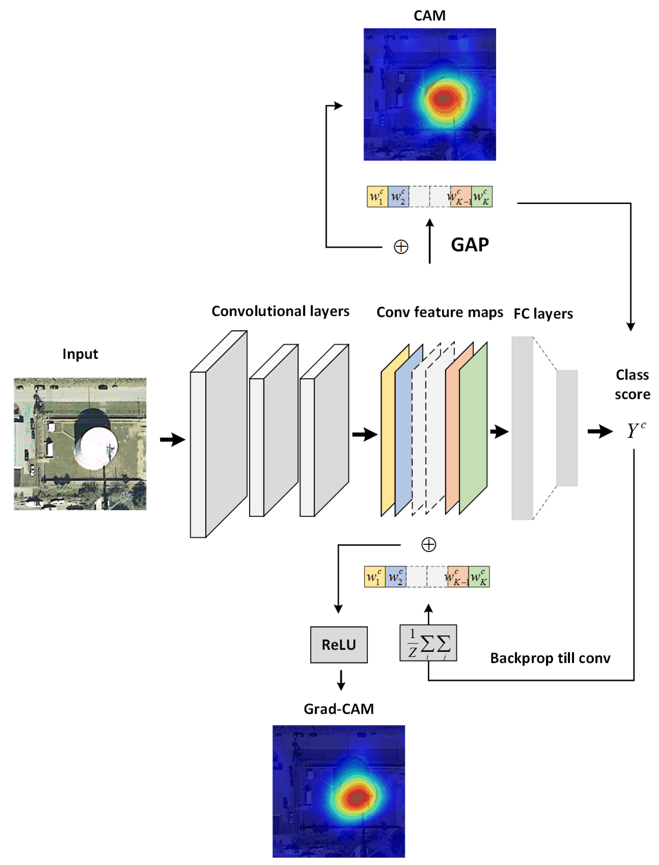
33] layer can not only be used as regularizing training but also locate deep representation that exposes the implicit attention of CNNs on an image. The CAM for a particular category was proposed by combining convolutional feature maps to indicate the discriminative image regions. Given a network architecture, the layers after last conv-layer are removed. A GAP layer is added after the convolutional feature maps and the spatial average of feature map of each unit is output to compute regression or other losses. Similarly, the weighted sum of the last convolutional feature maps is calculated to obtain class activation maps.
Specifically, for a given image of class
c, let
indicate the activation of the
k-th unit in the last convolutional layer at location
. The feature map after global average pooling
is
. Thus, the input to the softmax
is calculated as
where
denotes the weight corresponding to class
c for
k-th unit. To a certain degree,
is considered as the importance of
for class
c, so the class activation map
of each pixel for class
c is given by
It should be noted that actually describes the importance of the activation at location leading to the classification of the specific image to class c. Finally, the saliency map that reveals the most relevant regions to a particular category is obtained by upsampling the class activation map to the size of the input image.
2.2. Gradient-Weighted Class Activation Mapping
The CAM approach has an obvious drawback that it could only visualize the last convolutional layer, thus CAM is restricted to particular kind of CNN architectures performing global average pooling over convolutional maps immediately prior to prediction. Moreover, the change in architectures may cause damage to the network performance. An advanced approach called gradient-weighted class activation map (Grad-CAM), which is applicable to any CNN-based model, was proposed in [
28]. For those kinds of fully convolutional architectures, Grad-CAM can be reduced to CAM.
For a given image of class
c, let
and
represent the feature map of the
k-th unit and the final score before softmax respectively. First, the neuron importance weights
in Grad-CAM is redefined by computing the gradient of score for class
c as:
where
Z is the total number of pixels in the activation map. This weight
represents a partial linearization of the deep network downstream from
A, and also indicates the importance of
for class
c. Next, each spatial location in the specific class saliency map is calculated as:
Specifically, a Relu operation is applied to the linear combination of maps because features with a positive influence on a specific class are of interest. To obtain fine-grained pixel-scale saliency maps, is similarly upsampled to the size of the input image.
We illustrate the flow chart of applying CAM and Grad-CAM in visualizing the explanation map of a storage tank image in
Figure 2.
3. Proposed Method
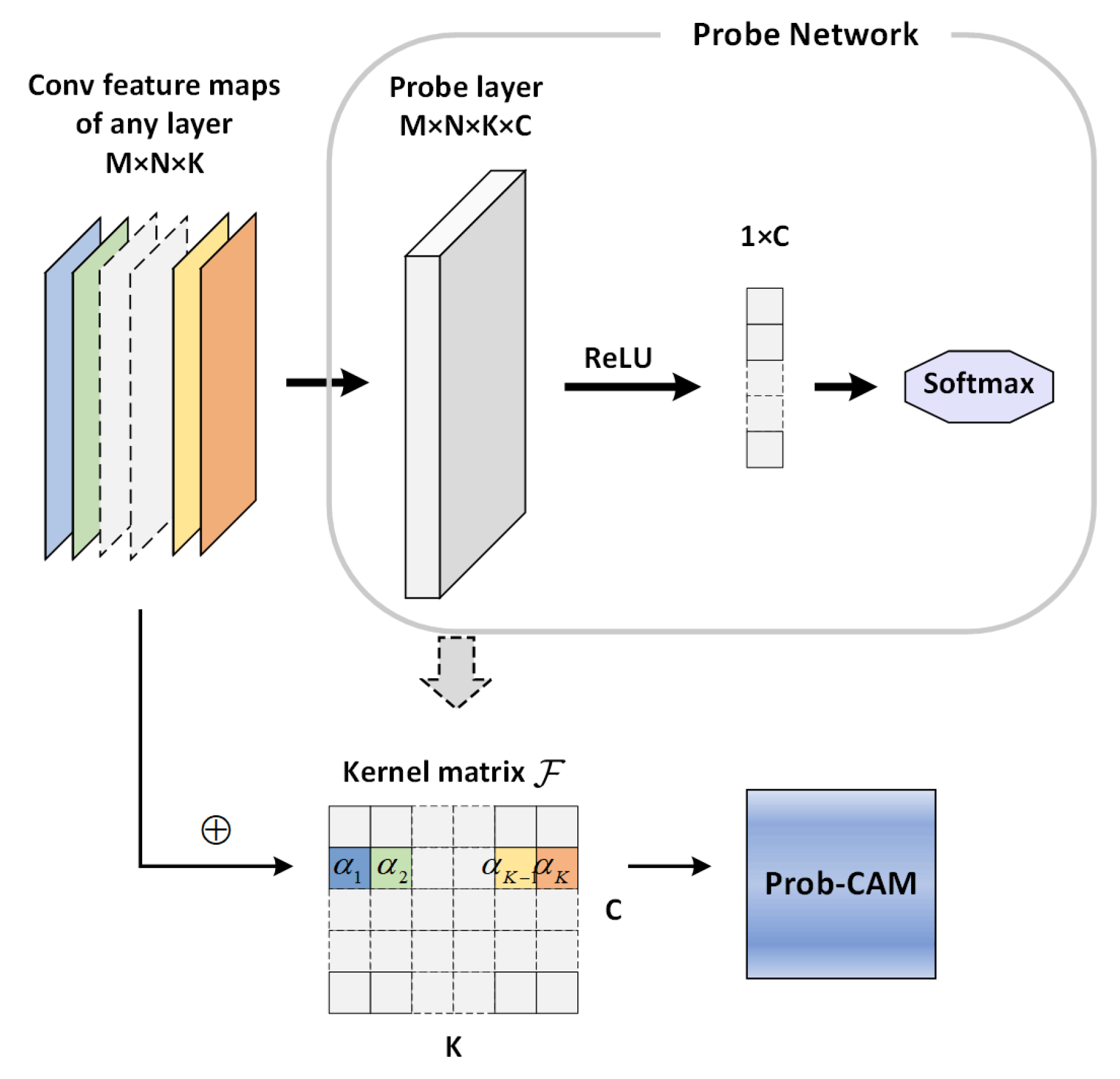
3.1. Probe Network
In accordance with the characters mentioned above, let A represent the feature map of an input image with class c. Specifically, denotes the feature map after the k-th unit in l-th convolutional layer, where indicates the size of the feature map.
When studying the visual explanations of
l-th convolutional layer, as shown in
Figure 3, a probe network composed of a probe layer, a ReLU layer and a softmax layer following behind are built and trained. The feature maps of
l-th convolutional layer are employed as input data and the output of the probe network is also the category number. The proposed probe layer is a conventional 2d-convolution. For this to occur, the size of kernel matrix
of the probe layer should be set as
, where
K and
C denote the depth of
l-th convolutional layer and the total number of categories, respectively. The score input to the softmax
, where ⊗ denotes the convolution operation. Thus, the output of the softmax for class
c is
.
To some extent, the concept of probe layer is similar to the global average pooling layer. It not only plays a role as regularizing training but also keeps the spatial location of the potential salient target. Furthermore, the probe network is more lightweight owing to the lack of a need for another fully-connected layer for final score. The weights of class
c in probe layer imply the importance of the input feature map
for the current class. The weight is computed as the average value of the
k-th unit for class
c.
Subsequently, the salient region map for each spatial location of class
c is performed as a weighted combination of feature maps after
l-th convolutional layer
The size of the achieved saliency map is the same as that of a feature map with , but each unit is supposed to be activated within its receptive field. The at different spatial locations forms a heat map of the current convolutional layer, so enlarging the heat map to the original image size can help obtain more details of the target, making it more intuitive and comprehensive for humans. Finally, the visual explanation image is obtained by simply upsampling the heat map.
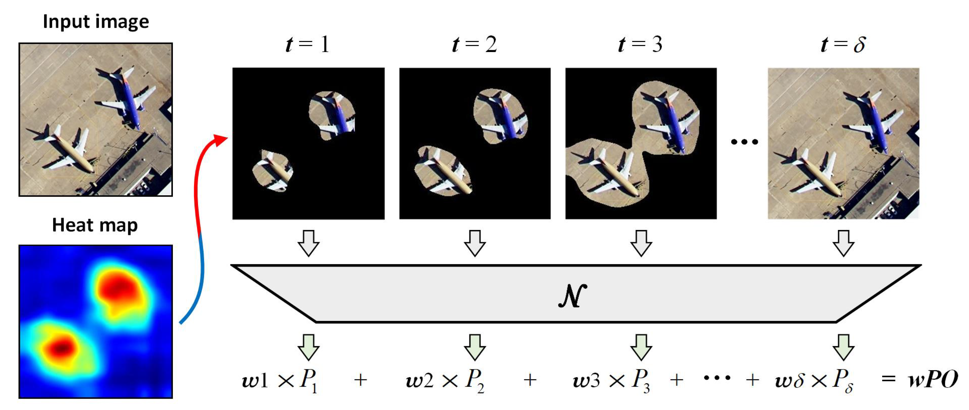
3.2. Weighted Probability of Occlusion
The visual saliency maps of particular layers can be acquired by the proposed probe network, afterwards the next task is picking out the most appropriate layer in which the saliency map with a reasonably favourable explainable results. The concept of faithfulness is used for reference to address this problem. For visual explanation, faithfulness is generally quantified by computing the difference of predictions between the saliency map and original image, where the saliency map is usually occluded or blurred to mask out high-energy regions. In the remote sensing image classification task, there are kinds of scene categories similar to texture images. Blurring leads will lead to the prediction of the blurred image; in particular, largely blurred images tend to fall into several specific categories. Consequently, occlusion is implemented on saliency maps in this paper.
The weighted probability of occlusion (wPO) is proposed to evaluate the explanation effectiveness of each convolutional layer for different categories. The procedure of wPO is illustrated in
Figure 4; here, we take one specific layer for example. For each image
I, the pixels sorted by the score in the saliency heat map are equally divided into
portions. The original image is first all occluded, and then we compute the probabilities by recovering the high-score clean pixels portion by portion. It is noted that the probabilities here are computed by the original whole network. Thus, the probability of the
t times operation is
where
denotes the network inference, and
is the occluded image recovered by adding
clean pixels.
There is another factor that cannot be neglected: the high-scoring regions of the saliency map that embody the effect of visual explanation. Namely, these highlighted image regions imply the explainability of the algorithm. Therefore, the probabilities of occluded images with fewer high-score clean pixels should be given larger weights to enhance their impact. The weight for probability of
t time is defined as
. Finally, the wPO is computed as a linear combination of weighted probabilities
where
I denotes the images of a particular class. Besides,
.
At this point, the weighted probability of occlusion that corresponds to every class at each convolutional layer is available, and let represent it. l denotes the layer number of networks. A larger value means a better explanation result. For class c, the most favourable explanation layer .
4. Experimental Results
In this section, we evaluate the proposed method on two datasets designed for remote sensing image classification and three widely adopted CNNs. We first demonstrate the experimental setup in
Section 4.1, including introductions to datasets, implementation details, evaluation criteria, etc. In
Section 4.2, we first report the quantitative results of our algorithm on two datasets in detail. Then, we show the evaluation on faithfulness in
Section 4.3. Next, in
Section 4.4, the explainability is evaluated from two aspects, the intuitive visual presentation of results and the verification of localization capability. Finally, we separately show the explainability of shallow layers on the scene categories that are similar to the texture image in
Section 4.5. The influential and state-of-art visual explanation algorithms CAM, Grad-CAM, and Grad-CAM++ are implemented for comparison.
4.1. Experimental Setup
4.1.1. Datasets Description
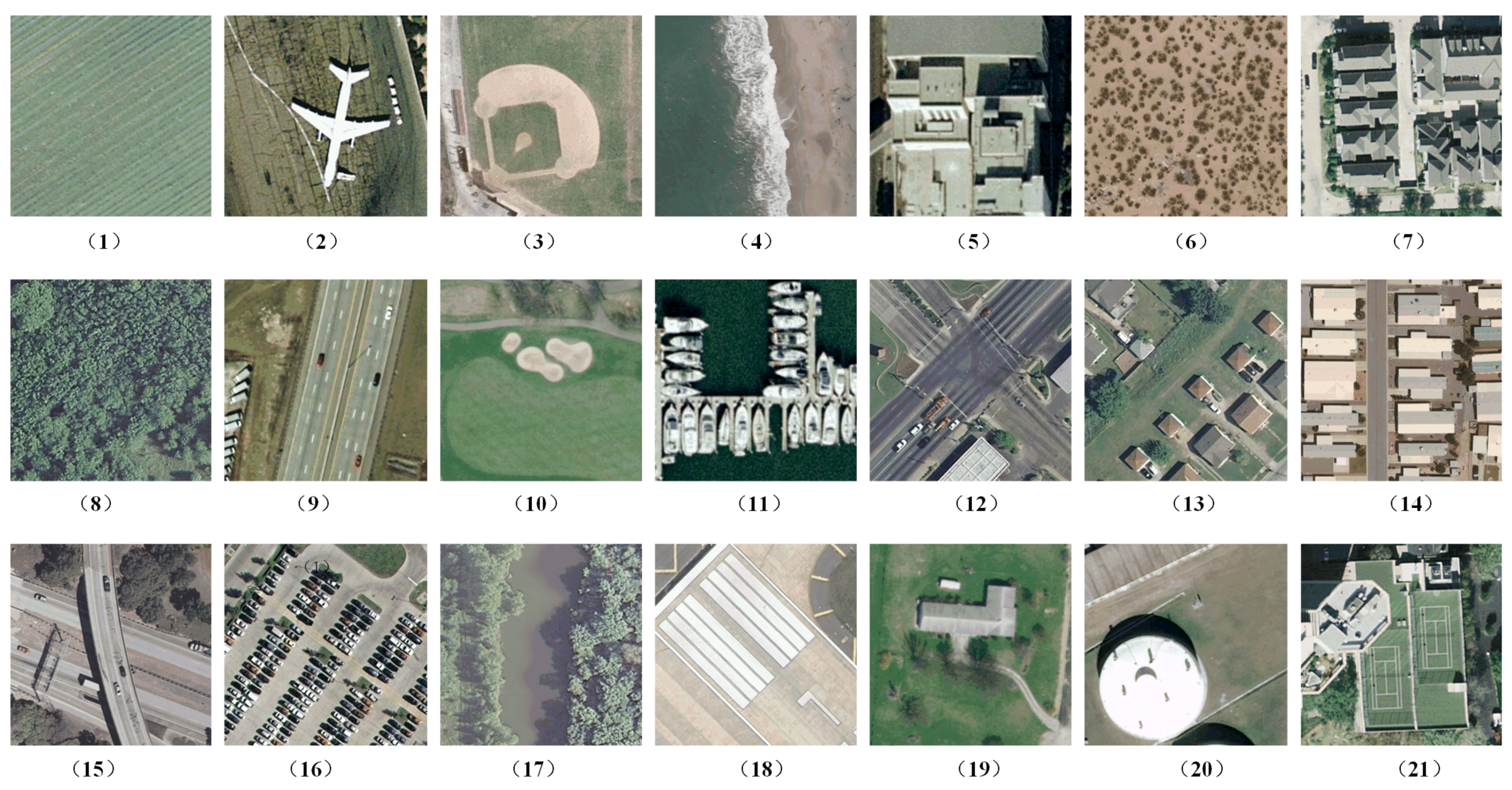
Two publicly available datasets designed for remote sensing image classification with a different quantity of images were adopted in our experiments. The first one is UC Merced land-use dataset which consists of images of 21 land-use scene categories selected from aerial orthoimagery with a pixel resolution of 1 foot [
34]. Each class contains 100 images with the size of 256 × 256 pixels.
Figure 5 shows some example images randomly selected from UCM. We implemented data augmentation, including flipping and rotating, owing to the limited amount of images. The other one is NWPU-RESISC45 dataset which are extracted from Google Earth (Google Inc., Mountain View, Santa Clara County, CA, USA) [
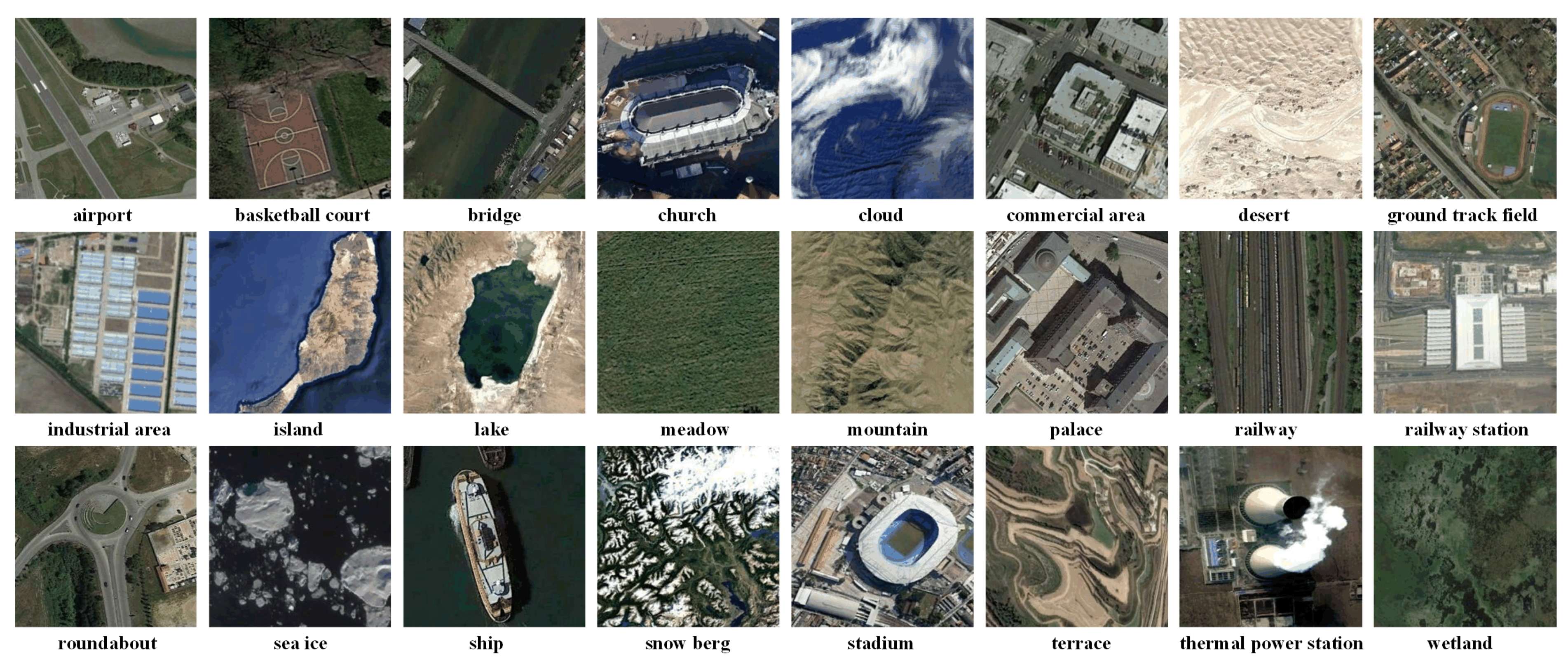
1], covering more than 100 countries and regions all over the world. The NWPU-RESISC45 dataset contains 31,500 images, containing 45 scene classes with 700 images in each class. Every image is 256 × 256 pixels in the red–green–blue (RGB) color space. The spatial resolution varies from about 30 to 0.2 m per pixel for most scene classes. Compared with UCM, NWPU-RESISC45 not merely covers the most categories of UCM, such as airplane, baseball diamond, forest, freeway, intersection, storage tank, etc., but also includes more generalized scene classification data such as commercial area, mountain, church, palace, cloud, sea ice, etc., making the classification task more challenging.
Figure 6 shows some example images from NWPU-RESISC45 with one sample per class.
4.1.2. Networks and Parameters Setup
We implemented three practical CNNs with different types of structures on the proposed framework: VGG-16 [
16], AlexNet [
15] and ResNet-50 [
35], and the corresponding numbers of convolutional layers are 5, 16, and 50, respectively. For VGG-16, we took ‘pool1’, ‘pool2’, ‘pool3’, ‘conv4-3’ and ‘conv5-3’ as examples to verify the ability of the proposed method, and ‘pool1’, ‘conv2’, ‘conv3’, ‘conv4’, ‘conv5’ are selected for AlexNet. For ResNet-50, we took ‘pool1’ and the last convolutional layer of each residual block, namely ‘conv2-3’, ‘conv3-4’, ‘conv4-6’ and ‘conv5-3’. When train the probe network, the feature maps directly after the pooling layer and the ReLU layer of the convolutional layer were employed as input.
The three networks are supposed to be re-trained on two remote sensing image datasets at first. The images were randomly divided into subsets for training, validation and testing. The ratios of UCM and NWPU-RESISC45 were set as 60%, 20%, 20% and 20%, 10%, 70%, respectively. These ratios and the identical images in respective subsets were also adopted in the period of training the probe network and computing the weighted probability of occlusion. All the networks including probe networks were trained using SGD [
36], with a batch size of 64. During re-training the networks, the initial learning rate was set to 0.05 and divided by 5 every 5 epochs, while the average value of the objective function over the validation set stopped decreasing. The training epochs for three networks are 40, 20 and 50, respectively. As for training of the probe networks, the initial learning rate was set to 0.001 and is divided by 5 every 5 epochs, while the training epochs was set to 20.
The weighted probability of occlusion (wPO) for each category was obtained on the training subsets. The only hyper-parameter in wPO was set to 32 in the following experiments.
4.1.3. Evaluation Criteria
The effectiveness of visual explanation is usually measured from two aspects: faithfulness and explainability. The faithfulness objectively evaluates the fidelity of the explanation to the judgment of the original model, while the explainability subjectively describes how much humans can understand the explanation results.
To quantify the faithfulness, two metrics proposed in [
37] were adopted in this paper: (i) Average Drop and (ii) Increase in Confidence. The Average Drop compares the average % drop in the model’s confidence of a particular category in an image. It is obtained by calculating the percentage of original probability occupied by the probability drop between original image and occluded image. Thus, a lower Average Drop means higher faithfulness. The Increase in Confidence considers another scenario, where the probability of the highlighted explanation map might exceed the original one. This index computes the proportion of abovementioned cases over the total number of images, so a higher Increase in Confidence is better. Note that these two evaluation indexes are gained on the testing subset.
Quantifying the explainability of algorithms on remote sensing image classification is tough because there is not a dataset that marks every distinct object in each scene category, and it is hard to mark a specific target in the scenes similar to the texture image. As a consequence, we evaluate the explainability from two aspects. First, considering that the explainability is a subjective measurement, we directly display the explanation maps generated by the proposed method and comparison methods as well. The gray level maps of salient heat maps corresponding to shallow layers are also shown to demonstrate the proposed algorithm’s explainability on scene categories similar to the texture image. Second, we refer to the measurement method in [
19,
28], a weakly supervised localization is implemented to indirectly verify the explainability.
4.1.4. Hardware Equipment
All the experiments were run on an HP Z8 workstation with two Intel Xeon Gold 5120 CPUs with 14 cores, two NVIDIA GeForce RTX 2080 Ti GPUs and a 128-GB memory.
4.2. Optimal Explanation Layer
In this subsection, we report the proposed weighted probability of occlusion (wPO) and generated optimal explanation layer achieved on two datasets and three networks. The wPO of each layer on UCM from VGG-16, AlexNet and ResNet-50 is shown in
Table 1,
Table 2 and
Table 3. The maximum wPO of each category in all layers is highlighted in bold and marked with a check mark for the ease of comparing. In the meantime, The optimal explanation layer from three networks for each class of NWPU-RESIS45 dataset is presented in
Table 4,
Table 5 and
Table 6 respectively. The wPO of NWPU-RESISC45 is not presented in detail because of paper length limits.
From these results, we made the following observations. First, not all scene classes identified the last convolutional layer as the optimal explanation layer, which proves the argument of this article. The scene classes containing clear objects of a large scale generally chose the last layer, such as airplane, storage tanks, tennis court and so on. In contrast, the scene classes similar to the texture image, such as agricultural, chaparral, forest and meadow, had the obvious trend that the explainability of the lower layer was stronger than the higher layer. Moreover, the middle layer was most likely to be chosen by the scene classes containing targets with a small scale, such as parking lot and mobile home park. This could be reasonably explained: the shallow layers in CNNs capture more detailed features, whereas the deep layers learn more holistic features of objects owing to the larger receptive fields. The kernels in the first convolutional layer usually represent texture information. Therefore, the low and middle layers provide more discriminative features for the abovementioned categories. In other words, the shallow layers are more suitable to be explained for these classes. The visual explanations are shown in the following subsections. Second, although there were small differences in some classes owing to the diversity of networks and datasets, the optimal explanation layer of identical class basically remained the same between different networks and datasets. This indicates that our argument possesses a certain universality. There are small differences in some classes on account of the diversity of networks and datasets.
4.3. Faithfulness
The quantitative evaluation on the faithfulness of the proposed Prob-POS and comparison methods is reported in this subsection. Two different metrics proposed in [
37] are adopted: (i) Average Drop and (ii) Increase in Confidence. For comparison, we implement CAM, Grad-CAM (GCAM) and Grad-CAM++ (GCAM++) on the two datasets and evaluate their faithfulness. Additionally, we also apply our proposed weighted probability of occlusion (wPO) selection strategy on Grad-CAM (GCAM&POS) and Grad-CAM++ (GCAM++&POS) to verify the effectiveness. It is noted that the Grad-CAM and Grad-CAM++ are implemented on the same retrained networks that are used by Prob-POS. Nevertheless, CAM changes the network architecture, so we sufficiently train the CAM networks according to the original reference on both datasets.
The results of faithfulness on the UCM and NWPU-RESISC45 dataset are shown in
Table 7 and
Table 8, respectively. The lower Average Drop and higher Increase in Confidence indicate the better faithfulness. It can be seen that the proposed Prob-POS achieved the best performance in both metrics and both datasets. This is because the Prob-POS chooses the layers with the highest explainability for each category and the fidelity of global explanation consequently outperforms the explanation methods that only concentrate on the last layer. When we only employed the proposed method on the last layer (Prob-CAM in the Table), the performance was also better than that of the comparison methods on two datasets with VGG-16. However, CAM achieved better faithfulness on AlexNet, a possible conjecture is that CAM adds another convolutional layer with 1024 kernels after original networks, enhancing the feature representation power of CNNs with a small volume, such as AlexNet, and so the explainability was boosted. In addition to the above two conclusions, the Average Drop and Increase in Confidence were both promoted by applying the wPO selection strategy on Grad-CAM and Grad-CAM++; hence, the wPO selection strategy is conducive to improving the faithfulness of visual explanation algorithms.
4.4. Explainability
Explainability subjectively describes how much humans could understand the explanation results. This is a direct metric evaluating the performance of a visual explanation algorithm. In this subsection, we respectively show the generated explanation maps from the last convolutional layer and middle-shallow layers to demonstrate the effectiveness of Prob-POS and Prob-CAM. If the salient regions of the generated explanation maps involve more specific semantic meanings, the explainability is higher.
4.4.1. Explainability of Last Layer
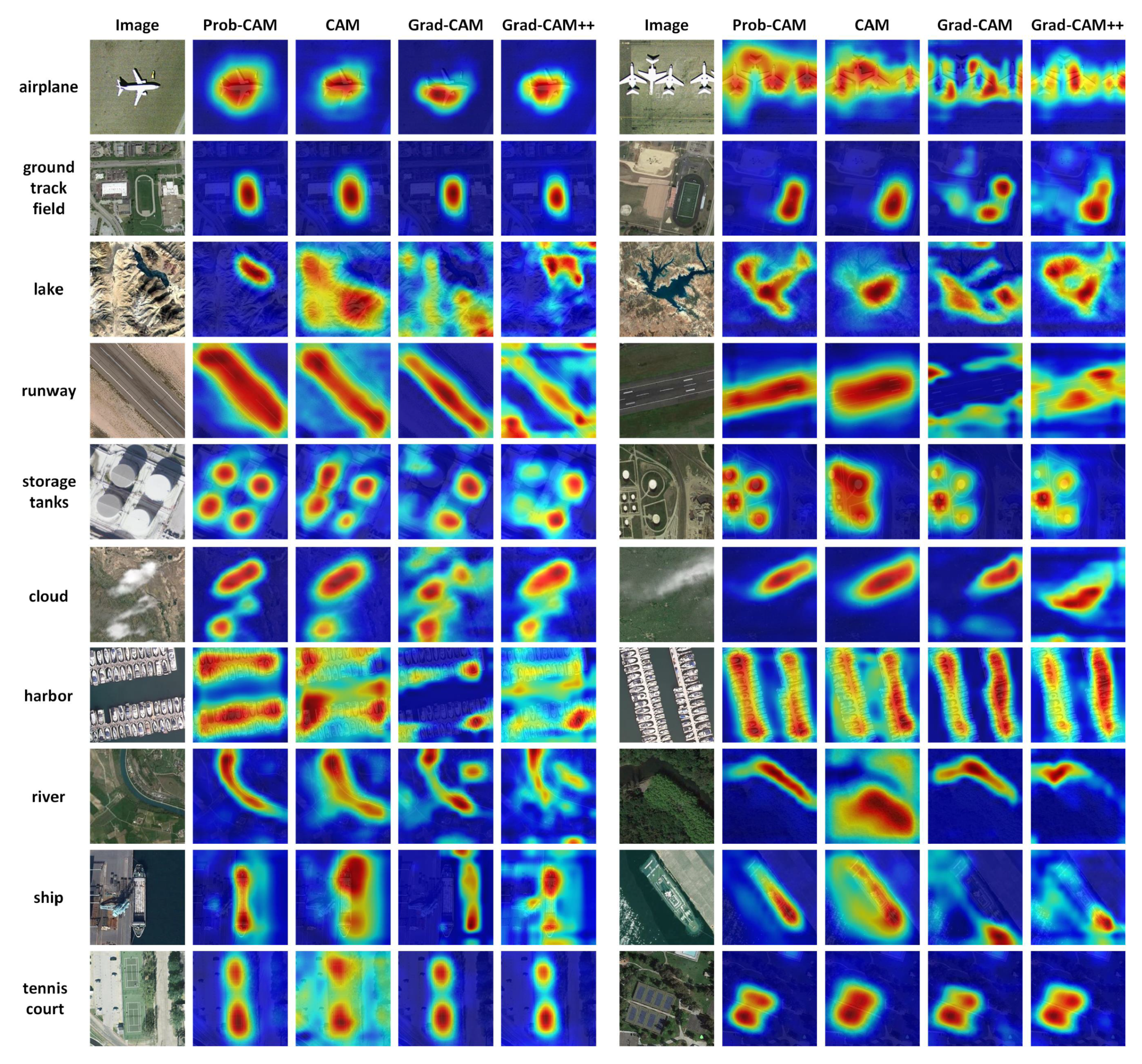
We sampled images whose optimal explanation layer was the last convolutional layer from UCM and NWPU-RESISC45 datasets, and display their corresponding explanation results on the last layer generated by the proposed Prob-CAM, CAM, Grad-CAM and Grad-CAM++ in
Figure 7. It can be observed that the explanation maps from the last layer mainly locate discriminative targets such as the airplane, the ground track field and the runway, or locate the whole area that contains many specific targets, for example, the pier berthing with rows of boats, shown in the harbor scene. These salient regions of the last layer are generally associated with targets of a relatively large scale.
Furthermore, the Prob-CAM achieved similar explainability as CAM, Grad-CAM and Grad-CAM++ on some scene classes, such as the airplane and the ground track field. However, in some categories, the explainability of Prob-CAM was better than that of the other three methods. For example, the salient region of runway generated by Prob-CAM includes more complete runway area than that of the others, and the explanation map on storage tanks generated by our method precisely locates four storage tanks, yet the location of CAM has errors, Grad-CAM and Grad-CAM++ both omit two storage tanks. On the whole, the explainability of Prob-CAM on last layer is equal to or better than the the other three methods on remote sensing images.
4.4.2. Explainability of Middle-Shallow Layer
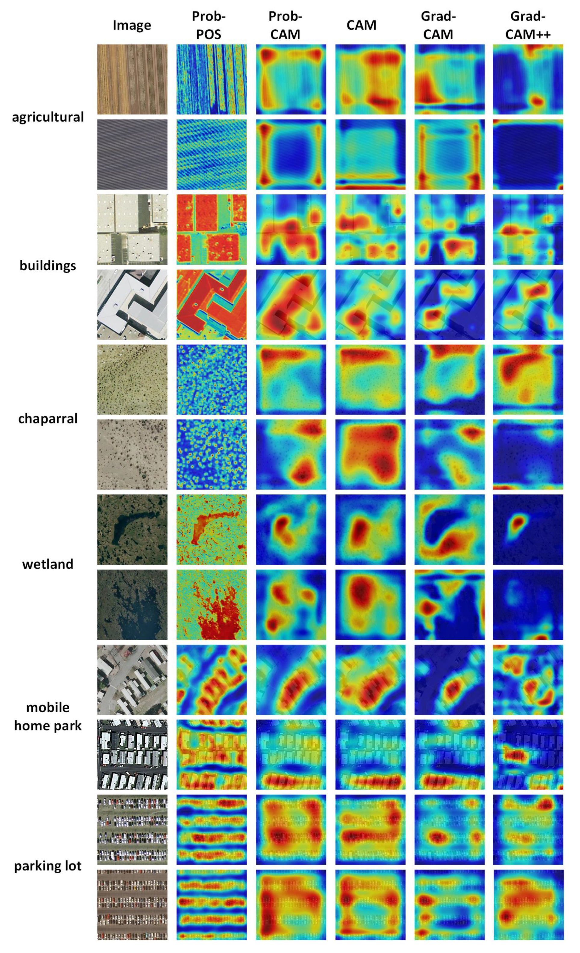
Similarly, we sampled images whose optimal explanation layer was the middle or shallow layer from two datasets. The results of corresponding explanation maps obtained by the proposed method and comparison methods are shown in
Figure 8, where the ‘Prob-POS’ indicates the explanation maps generated by the Prob-POS on the optimal explanation layer for each scene class, the ‘Prob-CAM’ refers to the explanation maps obtained by the Prob-CAM on the last layer, the ‘CAM’, ‘Grad-CAM’ and ‘Grad-CAM++’ also represent the explanation maps on last layer. The following conclusions could be drawn by observing these results.
First, the explanation maps generated by the proposed method on shallow layer could provide higher explainability for specific scene classes such as agricultural, chaparral and wetland. As shown in
Figure 8, the explanation maps on the shallow layer clearly depict the texture information for above mentioned scene images. Compared with the jumbled and irregular salient regions of explanation maps on the last layer, the results of shallow layer are obviously more understandable for humans in visual appearance. Moreover, there was a surprising phenomenon where the buildings scene that contained apparent targets of a large scale identified the shallow layer as the optimal explanation layer. We give a possible conjecture that the buildings are extremely regular shapes so the marginal information learned by shallow layers could represent these shapes more properly.
Second, the scene classes that contain plenty of targets of a small scale were better visually explained on middle layers. As shown in
Figure 8, the mobile homes in the mobile home park and the cars in parking lot are precisely located in the explanation maps on the middle layer, yet the salient regions in explanation maps on the last layer omit more or fewer targets, depending on methods applied. Considering the two points mentioned above, we may draw another conclusion that the explanation maps on last layer trend to describe centralized salient regions, whereas the tiny discrete objects and detailed information are more likely described by explanation maps on middle and shallow layers respectively.
Finally, the ideal visual explanation results rely on understandable explanation maps generated by the Prob-CAM as well as the optimal explanation layer chosen by the wPO selection strategy. These two aspects jointly verify the effectiveness of the proposed Prob-POS framework.
4.4.3. Evaluating Localization
In order to provide quantitative comparison results on explainability, we referred to the operations in [
19,
28] and performed a weakly supervised localization in the context of scene classification. The localization capability helps to indirectly reflect the explainability. Here, we took VGG-16 as the backbone to implement the experiment. The NWPU-RESISC45 dataset was used as the training dataset. The NWPU VHR-10 dataset [
38], which is a publicly available 10-class geospatial object detection dataset, was used for testing. Except from vehicle class, the other nine classes of NWPU VHR-10, which are airplane, ship, oil tank, baseball diamond, tennis court, basketball court, ground track field, harbor and bridge, are all included in the NWPU-RESISC45 dataset.
When inputting a testing scene image, to generate bounding boxes from explanation results, we also used a simple thresholding technique to segment the saliency heatmap. First, the regions of which the value is above 20% of the max value of the heatmap were segmented. Then, the bounding boxes were drawn on the segments that cover the connected component. We performed this procedure on the proposed Prob-POS and comparison methods, respectively. Note that the explanation heatmap of the Prob-POS was generated from the optimal convolutional layer. The comprehensive metric average precision (AP), in which the area overlap ratio was set to 0.5, was adopted to measure the location performance. The experimental results are shown in
Table 9.
It can be observed that the Prob-POS shows the best localization capability in most scenes. In the scenes of ship, oil tank and harbor, the Prob-POS achieves clear advantages. These quantitative compasison results further verify the explainability of Prob-POS. It should be noted that the average precision in this experiment is generally lower than that with the method designed for object detection. This is because there are many factors we had not taken into account, such as the diversity of scale and the segmentation of dense objects. But this implementation is capable and fair to verify the explainability.
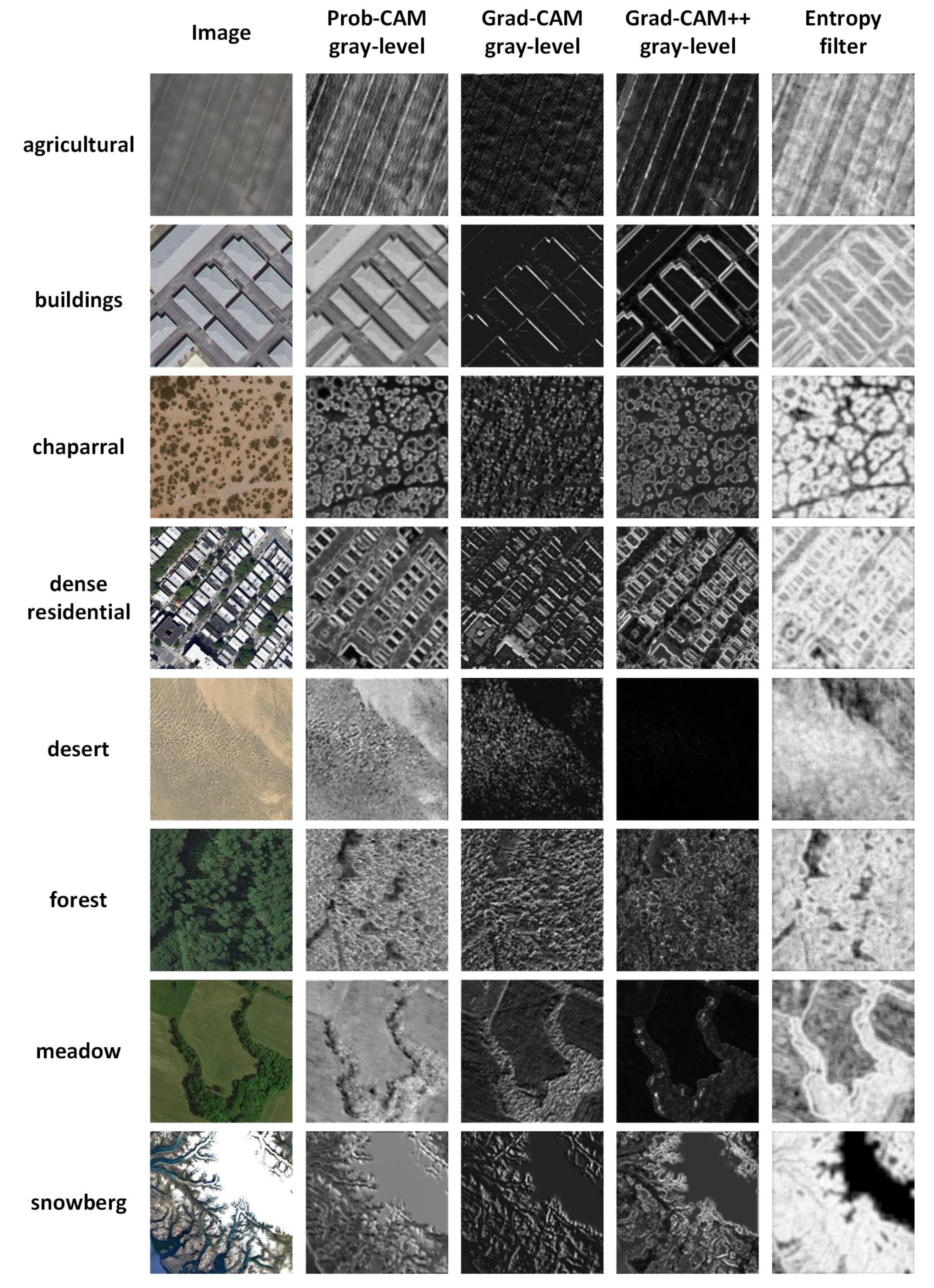
4.5. Explainability on Texture Information
To further demonstrate explainability on texture information of the explanation maps obtained by the proposed method, we simply display the gray level maps of Prob-CAM on the shallow layer of networks. Just like the above operation, here we also sampled images whose optimal explanation layer was first layer from corresponding networks. The results are shown in
Figure 9. We took the gray level maps generated by Grad-CAM, Grad-CAM++ and the texture image obtained by the entropy filter for comparison.
It can be seen from
Figure 9 that the gray level maps of Pro-CAM show more clear and detailed texture information than the other methods on most scene classes. Although the gray level maps of Grad-CAM and Grad-CAM++ also present visual texture information, some detailed elements are missing, for example part of the buildings are hard to identify in the buildings scene and dense residential scene. In addition, the contrast of Grad-CAM and Grad-CAM++ is generally low, so the present images are fuzzy. This is because the hypothesis proposed in Grad-CAM and Grad-CAM++ is based on the final convolutional layer. However, the proposed Prob-CAM does not suffer from this limitation, and thus it works better on shallow layers.
5. Conclusions
In this paper, we proposed a framework for improving visual explanations of remote sensing images called Prob-POS. The framework consists of two parts, the class activation map based on probe network (Prob-CAM) and the weighted probability of occlusion (wPO) selection strategy.
First, we used the probe network, which is composed of a probe layer, a ReLU layer as well as a softmax, which is a simple but effective algorithm to elaborately discriminate between the feature maps with different classes. We utilized the weights of a particular class in a well-trained probe layer to linearly combine the feature maps, and then the Prob-CAM is obtained. The Prob-CAM can be applied to convolutional feature maps after any layer.
Second, we developed a metric called wPO to measure which layer was the most suitable to be explained for different class. The variational weights were added to the probability of occlusion considering that the high-scoring regions in the explanation map embody the explainability of the visual image. The wPO provided a quantitative evaluation of the explanation effectiveness of each layer for different categories, and further, the optimal explanation layer can be automatically picked.
Finally, extensive experiments were carried out over publicly available datasets, UCM and NWPU-RESISC45, as well as the prevalent networks VGG-16 and AlexNet. The experimental results showed that the faithfulness of Prob-POS was better than that of other algorithms that only concentrated on the last convolutional layer. Moreover, the Prob-POS also achieved better explainability on remote sensing images, as the proper layer was selected to generate explanation maps. Thus, compared with visual results on the last layer, the Prob-CAM on middle or shallow layers provided accessible visual explanation patterns for remote sensing scene images, especially scenes that contained plentiful small targets or were similar to the texture image.
Some aspects of this study need further research. First, the gradients in CNNs were shown to be helpful for locating distinct objects; thus, it is worth utilizing the gradients to assist in the generation of explanation maps. Second, the location ability of objects is generally used to compute the explainability in existing methods, yet this is infeasible in some remote sensing categories. Consequently, a quantified and fair metric should be proposed to evaluate the explainability of explanation algorithms for remote sensing images.


