Article

Assessment of Different Complementary-Relationship-Based Models for Estimating Actual Terrestrial Evapotranspiration in the Frozen Ground Regions of the Qinghai-Tibet Plateau

1
Cryosphere Research Station on the Qinghai-Tibet Plateau, State Key Laboratory of Cryospheric Science, Northwest Institute of Eco-Environment and Resources, Chinese Academy of Sciences, Lanzhou 730000, China
2
University of Chinese Academy of Sciences, Beijing 100049, China
3
Southern Marine Science and Engineering Guangdong Laboratory, Guangzhou 511458, China
4
Key Laboratory of Water Cycle and Related Land Surface Processes, Institute of Geographic Sciences and Natural Resources Research, Chinese Academy of Sciences, Beijing 100101, China
5
School of Water Conservancy Engineering, Zhengzhou University, Zhengzhou 450001, China
6
School of Geographical Sciences, Hebei Normal University, Shijiazhuang 050024, China
*
Author to whom correspondence should be addressed.
Remote Sens. 2022, 14(9), 2047; https://doi.org/10.3390/rs14092047
Submission received: 10 March 2022 / Revised: 14 April 2022 / Accepted: 21 April 2022 / Published: 25 April 2022

Abstract

:
Actual evapotranspiration (ETa) is important since it is an important link to water, energy, and carbon cycles. Approximately 96% of the Qinghai-Tibet Plateau (QTP) is underlain by frozen ground, however, the ground observations of ETa are particularly sparse–which is especially true in the permafrost regions–leading to great challenge for the accurate estimation of ETa. Due to the impacts of freeze-thaw cycles and permafrost degradation on the regional ET process, it is therefore urgent and important to find a reasonable approach for ETa estimation in the regions. The complementary relationship (CR) approach is a potential method since it needs only routine meteorological variables to estimate ETa. The CR approach, including the modified advection-aridity model by Kahler (K2006), polynomial generalized complementary function by Brutsaert (B2015) and its improved versions by Szilagyi (S2017) and Crago (C2018), and sigmoid generalized complementary function by Han (H2018) in the present study, were assessed against in situ measured ETa at four observation sites in the frozen ground regions. The results indicate that five CR-based models are generally capable of simulating variations in ETa, whether default and calibrated parameter values are employed during the warm season compared with those of the cold season. On a daily basis, the C2018 model performed better than other CR-based models, as indicated by the highest Nash-Sutcliffe efficiency (NSE) and lowest root mean square error (RMSE) values at each site. On a monthly basis, no model uniformly performed best in a specific month. On an annual basis, CR-based models estimating ETa with biases ranging from −94.2 to 28.3 mm year−1, and the H2018 model overall performed best with the smallest bias within 15 mm year−1. Parameter sensitivity analysis demonstrated the relatively small influence of each parameter varying within regular fluctuation magnitude on the accuracy of the corresponding model.

Graphical Abstract

1. Introduction

Terrestrial evapotranspiration (ET) is an important part of the water cycle and surface energy balance, which is not only the nexus of the water cycle in the soil–vegetation–atmosphere continuum, but also a crucial link in the mass exchange and energy balance of the land surface [1,2]. Accurate estimation of ET is important to deeply understand how much liquid or solid water from land transforms as vapor in the atmosphere, which has significant implications for regional weather or climate conditions, and water resource management, such as ecological conservation and agricultural management, etc. [3,4,5].
In practice, ET estimation is often challenging because of complex land–atmosphere interactions, which often involve relevant micrometeorological, hydrological, or ecological methods [6,7]. In recent decades, great progress has been made on the theories and technologies of actual evapotranspiration (ETa) regardless of observations or simulations, significantly contributing to our knowledge of the ET process [8,9,10,11,12]. Current ET estimation approaches, such as land surface models or remote sensing technologies, have been successfully applied to various climatic or ecosystem zones [13,14,15]; however, the above approaches generally have relatively higher uncertainty in parameterization schemes at specific zones and require detailed information on vegetation or soil properties [16], which is especially difficult for data-scarce regions. For example, the Penman-Monteith (PM) [17,18] equation is often used to calculate potential evapotranspiration (ETp), which is close to ETa under ample water supply conditions, and with a higher accuracy. However, under water-limited conditions, the PM method assumes typically that ETa is proportional to the ETp (rescaling with soil moisture content), giving rise to practical difficulties such as soil moisture data unavailability in harsh environments where the estimation has a higher uncertainty. In addition, the assumption of the positive relationship between ETa and ETp may be rejected by observational evidence that supports negative correlations between the two variables [19]. Han [20] emphasized that the correlation between ETa and ETp depends mainly on water availability rather than always being positive.
Bouchet [21] first proposed another important hypothesis about ETa estimation, often called the “Bouchet hypothesis”. In contrast to the PM method, Bouchet [21] described the negative relationship between ETa and ETp caused by land-atmosphere feedback, which is also referred to as the complementary relationship (CR) approach. The greatest advantage of the CR approach is that it does not require any vegetation and soil information, and only a few model parameters and routine meteorological forcing data are needed [22,23]. Various models based on the CR approach have been proposed over the past decades [24]. The most widely used CR-based models include the AA (advection-aridity) model [25], CRAE (complementary relationship areal evapotranspiration) model [26], and GG (Granger and Gray) model [27], which are all based on the linearly symmetric CR approach. However, some later studies [28,29] have found that the complementary relationships are not symmetric, and they further proposed various asymmetric linear CR-based functions. Nevertheless, Han [30] found that both symmetric and asymmetric linear CR-based functions have poor generality and are applicable only to some mild climate regions. To extend the applicability of the CR function, Han [31] and Brutsaert [32] generalized the CR approach; subsequently, many studies have further refined the CR approach based on the above [33,34,35,36,37]. At present, various CR-based models have been applied to different ecosystems (shrubland, cropland, grassland, etc.) or climate (arid, semiarid, temperate) regions around the world on annual, monthly, daily, and sub-daily timescales [38,39,40,41,42], but very few studies focused on frozen ground regions on the Qinghai-Tibet Plateau (QTP), which may limit the development and application of the CR approach in frozen ground regions.
The QTP accounts for approximately a quarter of China’s land area, with an average altitude greater than 4000 m above sea level, known as the “roof of the world” and the “third Pole” [43]. Its vast topography and high altitude have significant impacts on the weather and climate of East Asia and even the world through thermal and dynamic forcing [44,45]. Additionally, frozen ground is widely distributed on the QTP [46], accounting for 96% of the area (including approximately 40% permafrost and 56% seasonally frozen ground). In these regions, freeze-thaw seasonal cycles and permafrost degradation [47,48] have certainly affected the regional hydrothermal balance of the soil–vegetation–atmosphere system; however, one of the current obstacles is that little is known about how seasonal and long-term ETa rates have changed in the frozen ground regions. In recent decades, several comprehensive observation sites have been established [49,50], improving our understanding of the ET process, but large-scale ETa estimation in the frozen ground regions of the QTP is still sparse. Hence, the above CR approach using only routine meteorological observations seems to be a feasible method. Wang [51] have improved and validated one CR-based model when applied to a permafrost sites on the QTP, but it is still unclear about which CR-based models are best for ETa estimation in this region.
This study utilized four comprehensive field sites, which are all located in the frozen ground regions of the QTP, based on five CR-based models with in situ measurement meteorological and eddy-covariance (EC) flux data, to calculate variables and optimize parameters in CR-based models. The objective of this study was to clarify the applicability of five widely used CR-based models in the frozen ground regions of the QTP and further investigate the uncertainty of the CR approach in ETa estimation. The results of this study could provide a reference for the applicability of CR-based models in the frozen ground regions of the QTP and provide a simple and feasible option for future large-scale terrestrial ETa in such data-scarce regions.

2. Materials and Methods

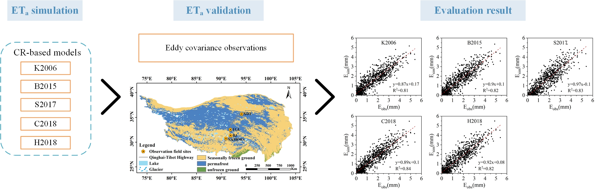
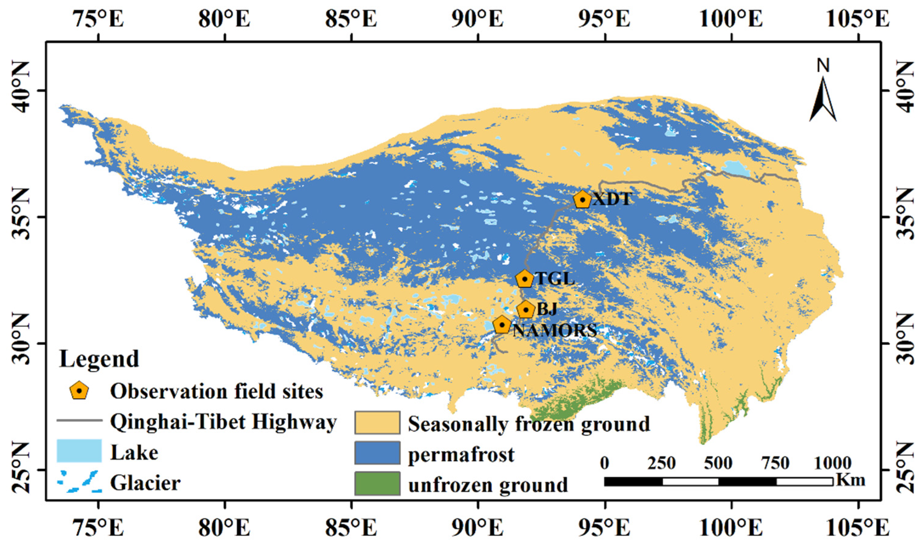
2.1. Site Description

In this study, in situ measurement data were collected from four comprehensive observation field sites (Figure 1). Tanggula (TGL, 91.86°E, 32.58°N, 5100 m asl) and Xidatan (XDT, 94.13°E, 35.72°N, 4538 m asl) lie in the south edge and northern limit of permafrost regions of QTP, covered by alpine steppe and alpine meadow, where the annual average air temperature is about −4.7 °C and −3.6 °C, and the annual accumulated precipitation is about 352 and 384.5 mm, respectively [52]. Another two field sites, Nagqu (BJ, 91.90°E, 31.37°N, 4509 m asl) and Nam Co (NAMORS, 90.96°E, 30.77°N, 4730 m asl), lie in the seasonally-frozen ground regions of QTP, covered by alpine meadow and alpine steppe, where the annual average air temperature is about 0.54 °C and −0.36 °C, and the annual accumulated precipitation is about 436 and 462 mm, respectively [53]. All the sites are near the Qinghai-Tibet highway.

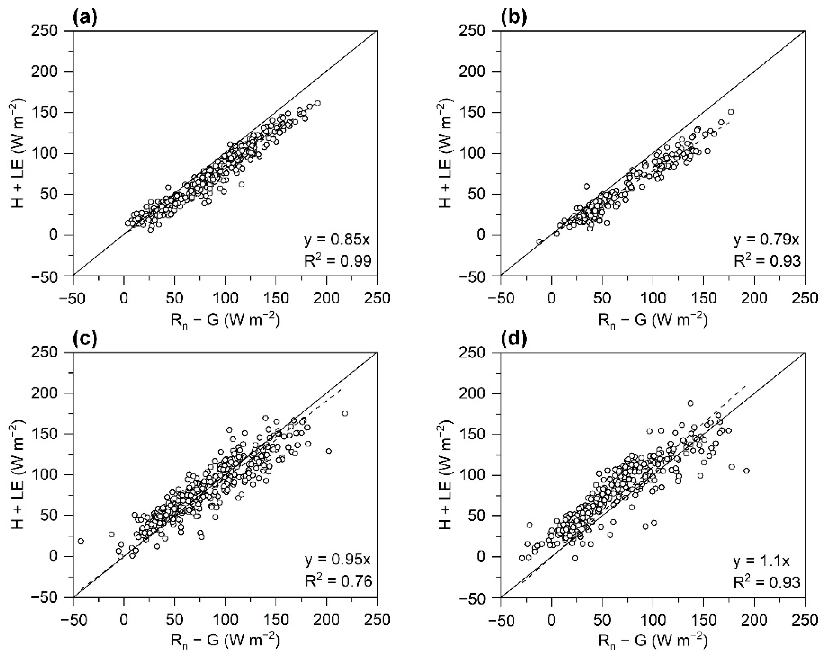
2.2. In Situ Measurement Data and Data Processing

All four selected field sites include eddy covariance flux data, meteorological data, soil temperature, soil moisture content, and soil heat flux data in a shallow soil layer. Eddy covariance flux data, including latent heat flux (LE) and sensible heat flux (H), were used to identify the performance of the different CR-based models. All EC systems were installed on towers about 3 m distance from the ground, consisting of a three-dimensional sonic anemometer (CAST3, Campbell Scientific Inc., USA) that measured instantaneous horizontal (u,v), vertical (w) wind speeds and sonic air temperature fluctuations, and an open path infrared gas analyser (Li-7500, LI-cor Inc., USA) that measured the water vapor density and carbon dioxide concentrations fluctuations. The EC instruments were all sampled at a frequency of 10 Hz. The corresponding meteorological data, including roughly 2 m downwards/upwards shortwave and longwave radiation, air temperature, relative humidity, wind speed, and pressure, were employed to drive each CR-based model. Soil temperature, soil moisture content, and soil heat flux data in shallow soil layer (within 10 cm from ground surface) were used to calculate ground heat flux for variables in CR-based models. All above observations were recorded at intervals of 30 min. Data of TGL and XDT were provided from Cryosphere Research Station on the Qinghai-Tibet Plateau, Northwest Institute of Eco-Environment and Resources, CAS (http://new.crs.ac.cn/, 1 September 2021). Data of BJ and NAMORS were provided from National Tibetan Plateau Third Pole Environment Data Center, CAS (https://data.tpdc.ac.cn/en/data/b9ab35b2-81fb-4330-925f-4d9860ac47c3/, 1 September 2021). In addition, two different selected study periods of each field site were determined by data integrity and continuity; observation of first and second year was taken as calibration and validation period, respectively.
The EC flux raw data processing was conducted on EddyPro7.0.6 software, and the main processing steps included spike detection, lag corrections of H2O/CO2 relative to the vertical wind component, sonic virtual temperature correction, coordinate rotation (planar fit rotation), corrections for Webb-Pearman-Leuning density fluctuations, and frequency response correction. The 30 min data output by EddyPro software was screened as follows: (1) the data of instrument error was removed; (2) 30-min record data with more than 10% missing values were excluded; (3) night data with weak turbulence (friction velocity (u*) less than 0.1 m s−1) were eliminated; (4) data with quality control code “2” (“2” indicate poor quality) were filtered out [54]. Then, half-hourly data during data available period accounts for filling the gaps; for gaps within seven consecutive days, they were filled using REddyProcWeb online tool (https://www.bgc-jena.mpg.de/bgi/index.php/Services/REddyProcWeb, 1 September 2021); for gaps longer than seven consecutive days, they were filled alternatively using aerodynamic method [55] or Bowen ratio energy balance method [56] for 30-min intervals. Finally, 30 min gap-filled flux data were aggregated into daily values. Ground heat flux were computed by linear method and thermal diffusion equation (TDE); detailed calculation processes are described in Yang [57] and Yao [58]. The daily energy balance closure ratios are 0.85, 0.79, 0.95, and 1.1 at TGL, XDT, BJ, and NAMORS, respectively (Figure 2).
It should be noted that on snow cover days, snow sublimation was one of the main evapotranspiration forms for four selected sites. Due to lack of observation of snow cover, this study employed the albedo instead, defined as the ratio of upward short wave radiation to downward shortwave radiation, to identify whether the observation field was snow-free or not. To exclude the influence of solar elevation angle, daily mean albedo was calculated as the average of half-hourly albedo from 10:00 to 14:00, local time. According to the variations of albedo at each observation fields, snow cover days were determined. In addition, snowfall still occurs during warm season at some observation fields, however, snow generally melts quickly to liquid water in few hours; thus, on a daily basis, only sublimation during cold season (from October to April in the next year) were considered. Then, the latent heat of vaporization—λv (J Kg−1), for snow free days—and the latent heat of sublimation—λs (J Kg−1), for snow cover days—were calculated using Equation (1), and the results were then used to calculate the actual evapotranspiration or sublimation [59]:
{ λ v = ( 2500 2.4 T a ) × 10 3 λ s = ( 2834.1 0.149 T a ) × 10 3
where Ta (°C) is the air temperature measured at 2 m high.

2.3. Complementary Relationship (CR) Approach

The CR approach involves three types of evaporation, namely, the actual evaporation (E, note: followed by “E” instead), the apparent potential evaporation (Epa), and the wet-environment evaporation (Epo). The CR approach is expressed as follows: for relatively larger and homogeneous surfaces with minimum advection, under certain net radiation inputs, E decreases with the availability of limited water over the underlying surface, and the energy that would be consumed by the latent heat flux thus becomes the sensible heat, thus increasing Epa. Hence, one can predict water-limited E by gauging how much Epa is raised from the hypothetical evaporation rate that should occur under the full wetness (Epo). Previous studies [60] hold that a unit decrease in E yields a corresponding unit increase in Epa, signifying a symmetric CR. This can be expressed as follows:
E p a E p o = E p o E
Epa and Epo is calculated as follows:
E p a = E r a d + E a e r o = Δ ( R n G ) Δ + γ + γ f ( U ) ( e o e a ) Δ + γ
E p o = α e E r a d = α e Δ ( R n G ) Δ + γ
where Erad is the radiation term, Eaero is the aerodynamic term, αe is an analog of the dimensionless Priestley-Taylor coefficient, (Rn − G) is the available energy (mm d−1), Δ is the slope of saturation vapor pressure curve at the air temperature Ta (kPa °C−1), γ is the psychrometric constant (kPa °C−1), and eo and ea are the saturation and actual vapor pressure of the air (kPa), respectively. f(U) (mm d−1 kPa−1) is the wind function calculated by Penman’s original empirical linear equation:
f ( U ) = 2.6 ( 1 + 0.54 U 2 )
where U2 is the measured wind speed (m s−1) at 2 m height.
Here, five CR-based models were selected to estimate E: the modified AA model [28] represents the linear CR version; the polynomial CR function [32] and sigmoid CR function [36] both represents the generalized nonlinear CR concept, and they represent different improved versions of the original CR approach mainly in physical boundary constraints; in addition, the calibration-free CR function and rescaled CR function are two improved versions based on the polynomial CR function [33,34,35].

2.3.1. Modified AA Model

The modified AA model extended the symmetric CR principle (herein referred to as K2006) and the equation becomes asymmetry as follows:
y K = b + 1 b x K 1 b
where b is a coefficient that depicts the proportion of the sensible heat that increases Epa, xK = Epo/Epa, yK = E/Epa. The only physical constraint is E ≤ Epo ≤ Epa; when the water availability of the landscape is not limited, E is assumed to proceed at Epa and E = Epo = Epa.

2.3.2. Polynomial Generalized Complementary Function

Brutsaert [32] reformulated a new general polynomial complementary function satisfying boundary conditions based on strictly physical constraints, referred to as the B2015 model, and its boundary conditions were as follows:
{ y B = 1 , x B = 1 y B = 0 , x B = 0 d y B d x B = 1 , x B = 1 d y B d x B = 0 , x B = 0
where xB = Epo/Epa, yB = E/Epa. The function form is as follows:
y B = ( 2 c ) x B 2 ( 1 2 c ) x B 3 c x B 4
c is an adjustable parameter which need to be locally calibrated.

2.3.3. Calibration-Free CR Function

Szilagyi [35] utilized the same function forms as the B2015 model (herein referred to as S2017), and the equation is as follows:
y S = 2 X S 2 X S 3
where yS is the same as yB, XS is defined as
X S = E p max E p a E p max E p o _ c E p o _ c E p a
Here two variables (Ep max and Epo_c) are introduced to improve the performance of S2017 function. Ep max is the maximum value that Epa can theoretically reach, which may appear when the air loses all moisture, that is,
E p max = Δ T d r y ( R n G ) Δ T d r y + γ + γ f ( U ) ( e o , T d r y 0 ) Δ T d r y + γ
where ΔTdry and eo,Tdry are the slope of the saturation vapor pressure curve and saturated vapor pressure, respectively, at extreme dry environment air temperature, Tdry (°C). Tdry can be estimated from the adiabatic line as follows:
T d r y = e o , T w b ( T a T w b ) e o , T w b e a + T w b
where Twb (°C) is the wet-bulb temperature, and eo,Twb (kPa) is the saturated vapor pressure at Twb. Twb is derived by another iteration of solving for the Bowen ratio during adiabatic changes, that is,
γ T w b T a e o , T w b e a = 1
Another one variable Epo_c is defined as
E p o _ c = α e E r a d = α e Δ w e a ( R n G ) Δ w e a + γ
where Δwea (kPa °C−1) is the slope of the saturation vapor pressure curve at Twes. Epo_c is the wet environment evapotranspiration rate calculated with Δwea instead of Δ. Note that S2017 function uses Epo_c instead of Epo because the latter variable is based on local air temperature, which is physically improperly employed to calculate wet environment evaporation. Szilagyi and Jozsa (2008) [61] suggested Equation (4) should use wet environment air temperature (Twea). Twea cannot be measured directly under water-limited conditions but can be approximated by the wet surface temperature (Twes). According to Szilagyi [62], Twes can be solved iteratively by implementing the Bowen ratio of a small wet patch, that is,
β w = R n G E p a E p a γ T w e s T a e o , T w e s e a
in which βw is the Bowen ratio of the wet patch (assuming that the available energy for the wet patch is close to that of the drying surface), and eo,Twes is the saturated vapor pressure at Twes(≈Twea). Note that Twes may be larger than Ta when air is close to saturation, and in such cases, Twea should be replaced by Ta.

2.3.4. Rescaled Complementary Function

Crago [34] used a similar method to the S2017 model, with Ep max introduced to rescale xB, and new analytical forms (herein referred to as C2018) have been proposed as follows:
{ x min = E p o _ c E p max X C = x x min 1 x min y C = X C
where yC are consistent with the corresponding variables of yS in the S2017 model.

2.3.5. Sigmoid Generalized Complementary Function

Han [36] brought in the minimum and maximum limits of Erad/Epen (xmin and xmax) under an assumed constant Erad and rederived four new boundary conditions fitting to two widely accepted assumptions following Penman’s combination theory, namely, dE/dEpen = 0 in extremely arid environments and E = Epen in completely wet environments. The boundary conditions are as follows:
{ y H = 0 , x H x min y H = 1 , x H x max d y H d x H = 0 , x H x min d y H d x H = 0 , x H x max
The following new sigmoid function in accordance with the above boundary conditions were also proposed (herein referred to as H2018):
y H = 1 1 + m ( x max x H x H x min ) n
where xH = Erad/Epen, yH = E/Epen, and the calculation of Erad and Epen (equal to Epa) refers to Equation (3); m and n are two unknown parameters that need to be locally calibrated.
{ n = 4 α ( 1 + b 1 ) ( x 0.5 x min ) ( x max x 0.5 ) x max x min m = ( x 0.5 x min x max x 0.5 ) n
where x0.5 is a variable that corresponds to yH = 0.5 (simply reflecting a temperate environment). Han [36] conducted that x 0.5 = 0.5 + b 1 α e ( 1 + b 1 ) , xmax and xmin can be simply set as 1 and 0 on a daily time scale, respectively. For longer time scales, xmax and xmin needed to be locally calibrated.

2.4. Model Parameter Calibration Methods

For the CR approach, one of the most important steps is to determine unknown parameter values. Generally, “optimal” parameter values could be either derived from transplanting from elsewhere, or are locally calibrated. First, “optimal” parameter values between two different sites are roughly equal under similar climatic or underlying surface conditions. In our study, the vegetation type of all four selected sites was grassland, so we set the “optimal” parameter values from other grassland sites reported in previous literature as the default values in each CR-based model. Note that the unknown parameters in the K2006, B2015, and H2018 models used corresponding values from the US-Fpe flux site [36] as default values, and the unknown parameters in S2017 and C2018 model used corresponding values from the Riggs Creek site at Australia [34] as default values, respectively. Second, unknown parameters of each CR-based model were all optimized by minimizing the root mean square error of the simulated and measured daily E during the calibrated period, and then the calibrated parameter values were used for the validation period.

2.5. Model Evaluation Criteria

To assess the model performance, five statistical metrics, including root mean square error (RMSE), mean absolute error (MAE), mean bias error (MBE), Nash-Sutcliffe efficiency (NSE), and correlation coefficient (CC) are used to evaluate the accuracy of simulated E with in situ measurements:
RMSE = 1 N i = 1 N ( E s i m , i E o b s , i ) 2
MAE = 1 N i = 1 N | E s i m , i E o b s , i |
MBE = 1 N i = 1 N ( E s i m , i E o b s , i )
NSE = 1 i = 1 N ( E s i m , i E o b s , i ) 2 i = 1 N ( E o b s , i E o b s ¯ ) 2
CC = i = 1 N ( E s i m , i E s i m ¯ ) ( E o b s , i E o b s ¯ ) i = 1 N ( E s i m , i E s i m ¯ ) 2 i = 1 N ( E o b s , i E o b s ¯ ) 2
where N is the number of observation, Esim,i (i = 1, 2, 3, …, N) is the simulated actual evapotranspiration value, Eobs,i is the observed actual evapotranspiration value, E s i m ¯ and E o b s ¯ are the mean values of Esim,i and Eobs,i, respectively.

3. Results

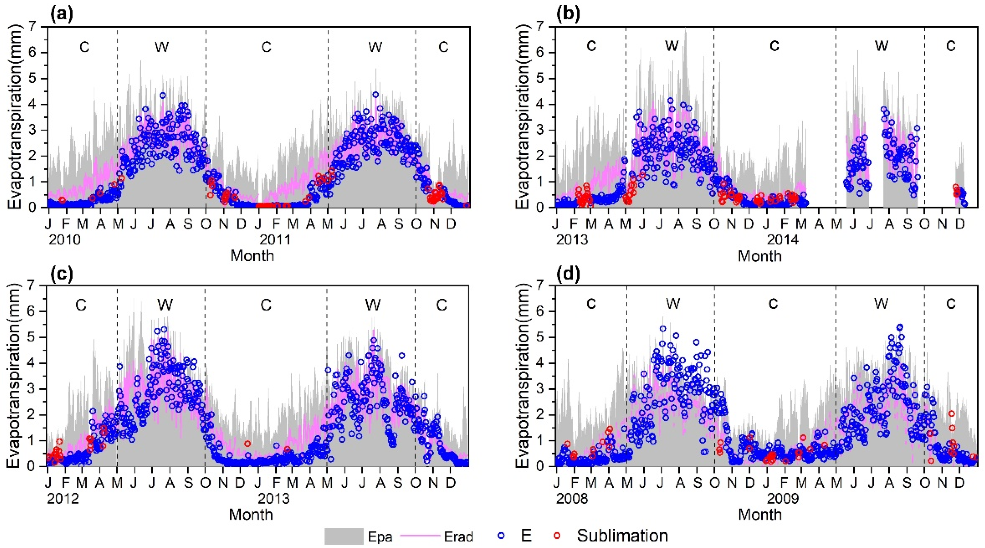
3.1. Variations in ET Rates at Four Observation Sites

The daily variations in actual evapotranspiration (E), sublimation, radiation term (Erad), and apparent potential evapotranspiration (Epa) rate at four observation field sites are shown in Figure 3. Note that relatively larger errors of observation may exist at NAMORS during some periods, especially in the warm season when E is larger than Epa, which is discrepant with Penman’s evaporation theory. Visibly, among four observation field sites–whether located in permafrost regions or seasonally frozen ground regions–are both clear seasonal variations of each ET variable: higher E and Epa usually occurs during the warm season, maximum E could reach approximately 4 mm d−1 at TGL and XDT, and 5 mm d−1 or more at BJ and NAMORS. For Epa, which exhibited greater daily fluctuations compared with E and Erad, the maximum Epa ranges from 5 mm d−1 to 7 mm d−1 at four selected sites: low E occurred during cold seasons and was generally close to zero when soils were frozen, except at NAMORS, and Epa and Erad was relatively lower, which was mainly controlled by net radiation. Additionally, some obvious differences between permafrost regions and seasonally frozen ground regions were that greater variations in E occurred at seasonally frozen ground regions than permafrost regions, and the onset time of increasing E after the frozen period in seasonally frozen ground regions (usually in late March) was earlier than that of permafrost regions (usually in late April), which was due to the onset time of thawing being earlier in the former. As the ground ice thaws, surface soil moisture increases, and E also increases.
Some studies found that E is larger than rainfall at the annual scale at observation sites on the QTP [59,63]; the same phenomenon was also found in our study (see Table 1). Due to missing values of rainfall during the study period at BJ and NAMORS, we instead used data from the nearby Naqu and Dangxiong country meteorological station provided from China Meteorological Administration. The exception of this was when there were observation errors about precipitation or ET; this phenomenon is often explained by surface soil moisture providing available water for evaporation. Although limited by land surface water supply, soil evaporation is one of the main forms of water consumption for the four selected field sites.

3.2. Evaluating Model Performance

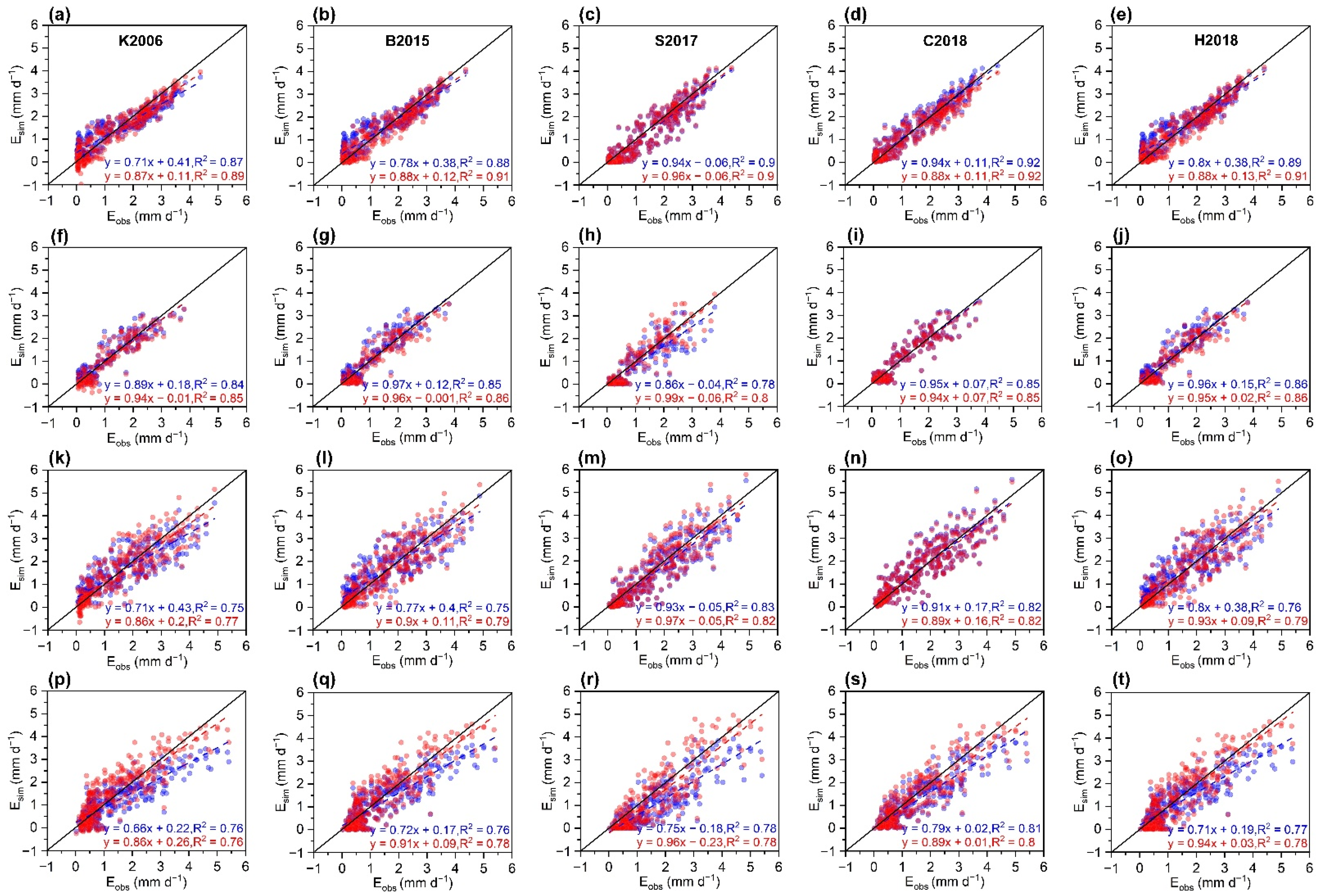
3.2.1. Model Performance with Default and Calibrated Parameter Values on a Daily Timescale

This study first employed the default and calibrated parameter values to simulate the daily actual evapotranspiration (Esim) and then compared with in situ measurements, respectively (Figure 4).
The results indicate that Esim was underestimated to different degrees by each CR-based model at all four selected sites, whether the default or calibrated parameter values were employed; the highest NSE value was 0.92 at TGL and the lowest NSE value was 0.58 at NAMORS. The average RMSE value was 0.4 mm d−1 at TGL and at XDT, 0.58 mm d−1 at BJ, and 0.63 mm d−1 at NAMORS when default values were employed (Table 2). After being locally calibrated, the highest NSE value was 0.92 at TGL and lowest NSE value was 0.69 at NAMORS. The average RMSE value was 0.36 mm d−1 at TGL, 0.38 mm d−1 at XDT, 0.56 mm d−1 at BJ, and 0.6 mm d−1 at NAMORS (Table 2), with only a small improvement in accuracy when compared with the results simulated by default parameter values. In addition, the CC values of five CR-based models all exceeded 0.87. Therefore, a better performance of the CR approach was found for daily E estimation in the frozen regions of the QTP, and unknown parameter values from other similar climatic or underlying surfaces could also be applicable without local calibration due to a lack of in situ measured E, such as in data-scarce regions.
However, a relatively larger bias occurred when there were lower E values for each model at all four sites, which indicated poor applicability of the CR approach. There were even some negative Esim values by the K2006 model when E was low at all four observation sites, probably because there were no strict boundary conditions constrained in the K2006 model, which led to abnormal values near the border of the boundary. In general, the CR approach may be inappropriate during the cold season in the frozen regions of the QTP because lower E values mainly occurred during the cold season. The S2017 model performed poorly among the five CR-based models, with relatively lower NSE values and higher RMSE and MBE values (Table 2), especially at NAMORS, where the MAE values reached 0.57 mm d−1 and 0.52 mm d−1 with the default and calibrated parameter values, respectively, signifying the largest bias during the study period. The C2018 model performed best at TGL, BJ, and NAMORS, and performed very well at XDT, and the NSE values of the C2018 model were all above 0.75. The overall performances of the B2015 and H2018 models were slightly inferior to that of the C2018 model, and the NSE and RMSE values of the above two models were close to those of the C2018 model.
Note that for the C2018 model, although there was only one unknown parameter to calibrate, there were more variables, such as wet and dry environment temperature, which meant a relatively more complex calculation process. For the B2015 model, previous studies have pointed out its deficiency in physical boundaries, which may be inappropriate for extremely dry or wet environments and periods. Therefore, the H2018 model, with relatively robust physical boundary constraints and a simpler calculation process, may be the most appropriate CR-based model for daily E estimation in the frozen regions of the QTP.

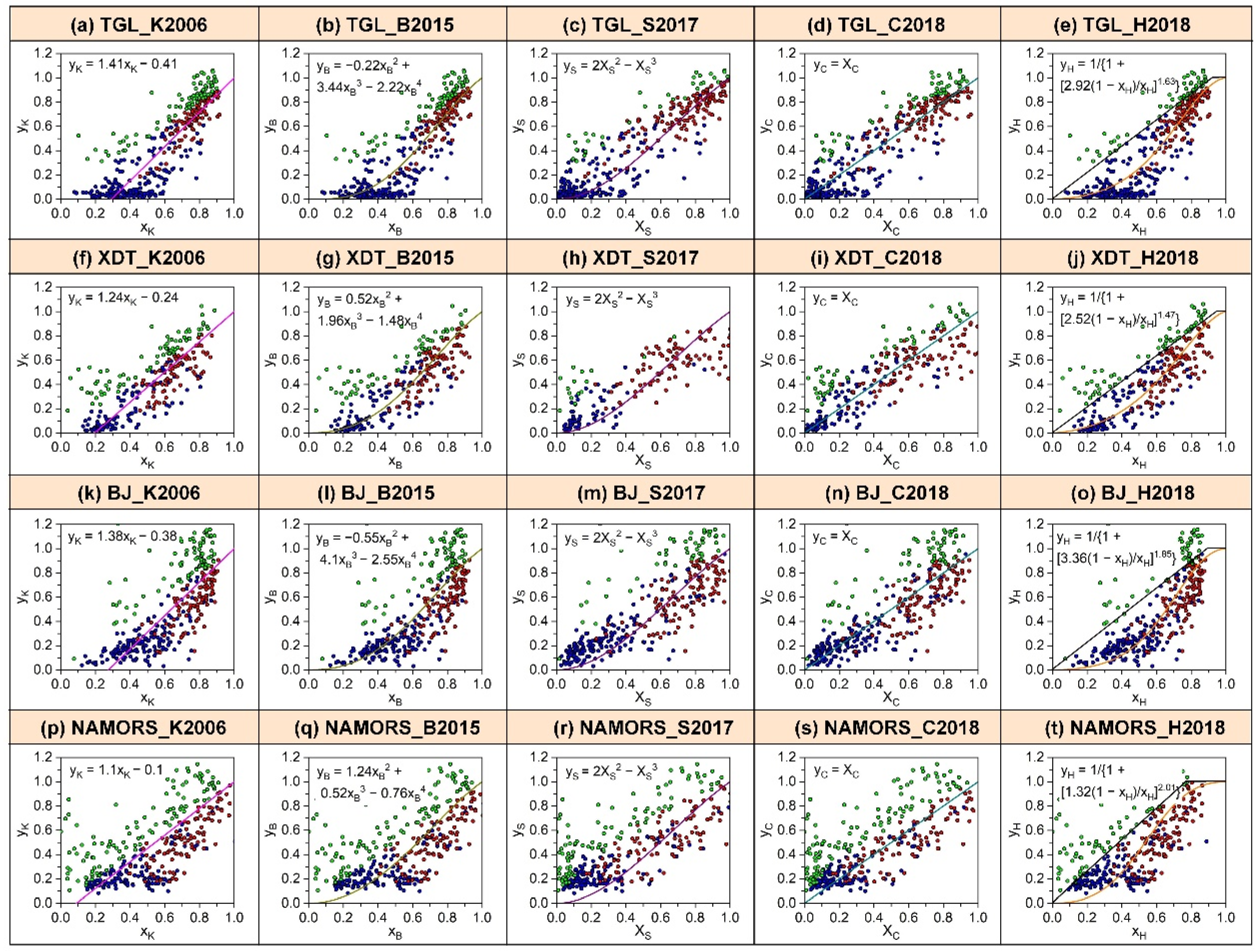
3.2.2. Performance of Different CR-Based Functions against Relationships among Three Evapotranspiration Variables

To determine relationships among three evapotranspiration variables (E, Epo and Epa) during warm and cold seasons and to further elucidate the applicability and optimal form of CR-based functions in the frozen ground regions of the QTP, the performance of different function forms using calibrated parameter values combined with observation data is presented in Figure 5. Here, all data at each field site were divided into three parts: daily ET variables that fulfill the preconditions of each CR-based model, judged by “po (Epo_c) ≤ Epa” for the K2006, B2015, S2017, and C2018 models, “EEpo and EEpen” for the H2018 model, and the above data can be used to further divide based on the warm and cold season, respectively. The remaining data are daily evapotranspiration variables that do not fulfill the CR-based models. Note that although parameter calibration was performed, there were still some data that did not satisfy the CR-based models, which may have been due to observation errors or inapplicability of the CR approach to that time.
The results indicated that observation data were unevenly scattered around CR-fitting lines at each site, and all CR-based function forms basically captured relationships among the three types of evaporation during the warm season in the frozen ground regions of the QTP, similar to the simulated results from some other sites around the world [36,42,64]. However, when variable y converges to 0 (that is, E is low), which often occurs in cold seasons, the dimensionless variable x (or X) has a relatively wide range, even above 0.6, because strong radiation (Erad) on the QTP leads to a high proportion of radiation to apparent potential evapotranspiration (Epa). Usually, a high proportion of radiation indicates there is strong evaporation energy available and higher actual evaporation; however, for water-limited frozen ground regions, water availability is another important factor affecting evaporation. Figure 5a–t shows relatively small deviations during warm seasons and the CR-fitting lines cross near the center of the observation data; five different CR-based functions both captured the daily E values well without evident differences, however, differences were clear in the lower E values. Because most studies about CR approach focus on warm seasons or growing seasons when E is relatively high, it is not enough to take into account the conditions of small E values during cold seasons; difficulties lie in high uncertainty of observation data during cold seasons, which leads to a lack of reliable data to validate whether the hypothesis of the CR approach is applied to cold and high-altitude areas or cold seasons from the aspect of the mechanism.

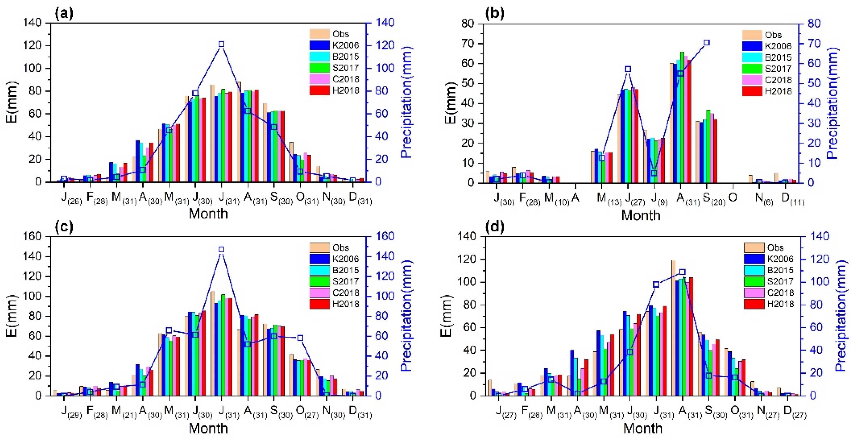
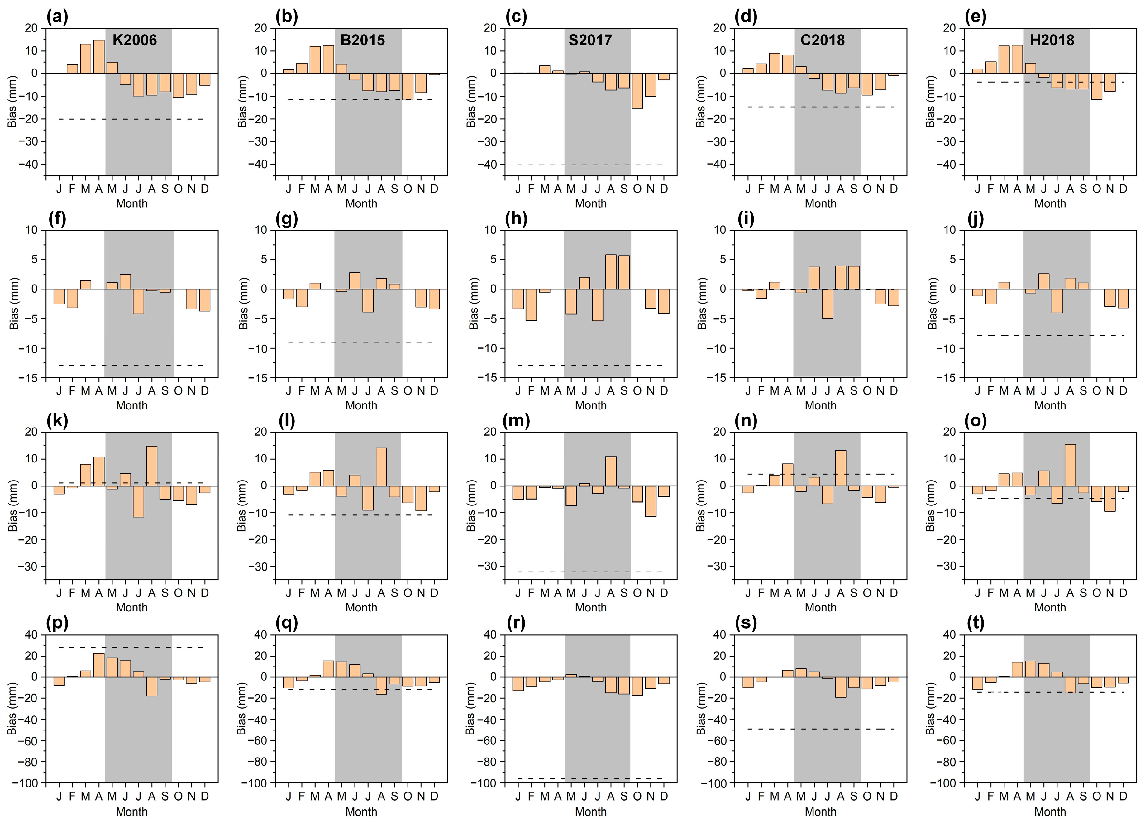
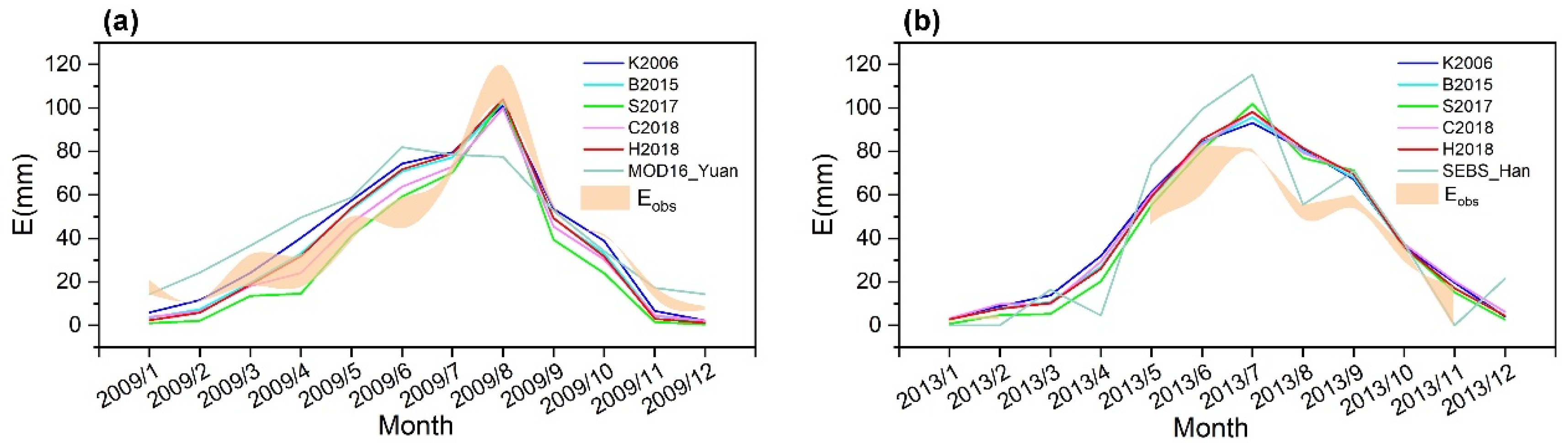
3.2.3. Model Performance with Calibrated Parameter Values on a Monthly Timescale

We also investigated the performance of five CR-based models with calibrated parameter values on a monthly timescale. Figure 6 illustrates that the monthly Esim got acceptable accuracy at TGL, XDT, and BJ, but relatively larger deviations occurred at NAMORS. The simulated performance between each CR-based model was very close, which indicated more stable performance to the CR approach on longer timescales. Compared with variations in precipitation, the peak of E was not always synchronized with the peak of precipitation on a monthly timescale. Taking TGL (Figure 6a) for an example, the peak of E occurred in August and was higher than concurrent precipitation; higher E may be contributed by water stored in the soil layer by antecedent precipitation, due to the peak of precipitation in July.
To further determine the contributions of monthly simulated bias to annual total bias at each field site, the monthly absolute bias of each CR-based model was calculated (Figure 7). Although the performance of the five CR-based models varied from one site to another, overall, the H2018 model seemed to have a smaller annual bias than the other models. According to Figure 7e,i,o,t, the H2018 model underestimated annual E at each site, and the bias was within 15 mm. The K2006, B2015, and C2018 models performed slightly inferior to the H2018 model; larger biases all occurred at NAMORS, and the rest of the sites performed relatively well. The S2017 model performed worst among the five CR-based models at each site, and the largest bias occurred at NAMORS, which was close to 100 mm on an annual timescale. Considering the contribution of monthly or seasonal bias to annual total bias (see Table 3), negative annual bias was mainly contributed by the negative bias of the warm season at TGL; however, the negative bias of the cold season contributed more to the total bias at XDT, BJ, and NAMORS. The larger negative monthly bias frequently occurred in October or November, and the maximum bias was −15.3 mm (in October) at TGL, −5.42 mm (in July) at XDT, −11.72 mm (in July) at BJ, and −17.58 mm (in October) at NAMORS.

4. Discussion

4.1. Uncertainty of Actual Evapotranspiration Estimation by the CR Approach

Using only routine meteorological variables (air temperature, relative humidity, wind speed, and net radiation) in the CR approach can better estimate daily or monthly E in the frozen ground regions of the QTP according to the present study; however, the uncertainty of the CR approach itself, physical variable calculations, and key parameter values are still non-negligible for estimating E on different spatiotemporal scales.
For the K2006 model, characterizing variables such as Epa and Epo is difficult. Although using the Penman equation to calculate Epa is widely accepted, determining Epo is controversial because a fixed analog of the Priestley-Taylor coefficient αe usually cannot vary with climate, which means that the value of αe cannot truly reflect the interaction between the land and atmosphere [65,66]. We also need to know atmospheric status–such as air temperature–under well-supplied water conditions at the land surface before determining Epo, despite some progress [61,62] that has been made in obtaining air temperature under well-supplied water conditions. However, usual iterative solving exists for unsolved or anomalous solutions, which makes it difficult to promote the above method as a universal approach.
For generalized complementary functions, in addition to the above common problems, the definition of boundary constraint conditions is another one important problem. Han [65] noted that boundary constraint conditions determine the domain of definition and the analytic formula of complementary functions. Many of the latest debates [67,68] on the CR-based functions have focused on boundary constraint conditions, which is controversial for the CR approach. The above-mentioned problems reflect a great lack of understanding of the evaporation process on different spatiotemporal scales for frozen ground regions on the QTP, where the current CR function forms seem to perform inferiorly in the specific regions described by Wang [42].
For the CR principle, an important prerequisite of the CR approach is that at large and homogeneous land surfaces, the influence of air advection could be negligible, so atmospheric evaporation demand is totally caused by feedback of the land surface. Morton [26] pointed out that the CR principle should be applied at spatial resolutions larger than 1 km and temporal resolutions longer than five days, since large-scale weather fronts may bring air masses over the land with a moisture signature decoupled from the underlying surface, which thus may temporarily disrupt the dynamic equilibrium of air humidity and surface fluxes in the land–atmosphere system. Although previous studies [28,38,42,69] have applied the CR approach to hourly or daily E estimations, the theory of the CR principle on short timescales still needs to be improved.

4.1.1. Influence of Parameter Values on Actual Evapotranspiration Estimation

Determining the parameter values of CR functions is urgent for the application of each CR-based model to estimate E, as well as for the development of a CR approach. The K2006 and H2018 both have two parameters, αe and b; the B2015, S2017, and C2018 all have one parameter, αe (note: parameter c in the B2015 model is an adjustable parameter, c = 0 often in most conditions, so, here we did not discuss parameter c). To determine the impacts of parameter values on evapotranspiration estimation, we discuss the following two problems: (i) difference in simulated results by each CR-based model with parameter calibration on different time lengths and (ii) parameter sensitivity for actual evapotranspiration estimation.
Here, we first investigated the influence of calibrated parameter values by different time lengths (whole year and warm season) on simulating daily E during the warm season. For the cold season, due to higher uncertainty of observations, we did not discuss the results here. Table 4 compares the parameter values and simulated NSE values during the warm season by the calibration period of one whole year and the corresponding warm season, respectively. The results indicated that the time length of parameter calibration did not have much of an impact on simulated E during the warm season, parameter αe was very close between the two calibration periods, and the differences in parameter b was slightly larger. According to our results, the simulated E was insensitive to the variations in parameter b in the K2006 and H2018 model, because even if the difference in parameter b was large, like the K2006 model at NAMORS, the simulated daily E between the two calibrated parameter values were still approximate. However, variations in parameter αe in all five CR-based models exerted more of an influence on the simulated results. The above results indicated that parameter calibration—especially αe—in CR-based models at specific sites is more important to simulate daily E compared with different time lengths of calibration periods in the frozen ground regions of the QTP.

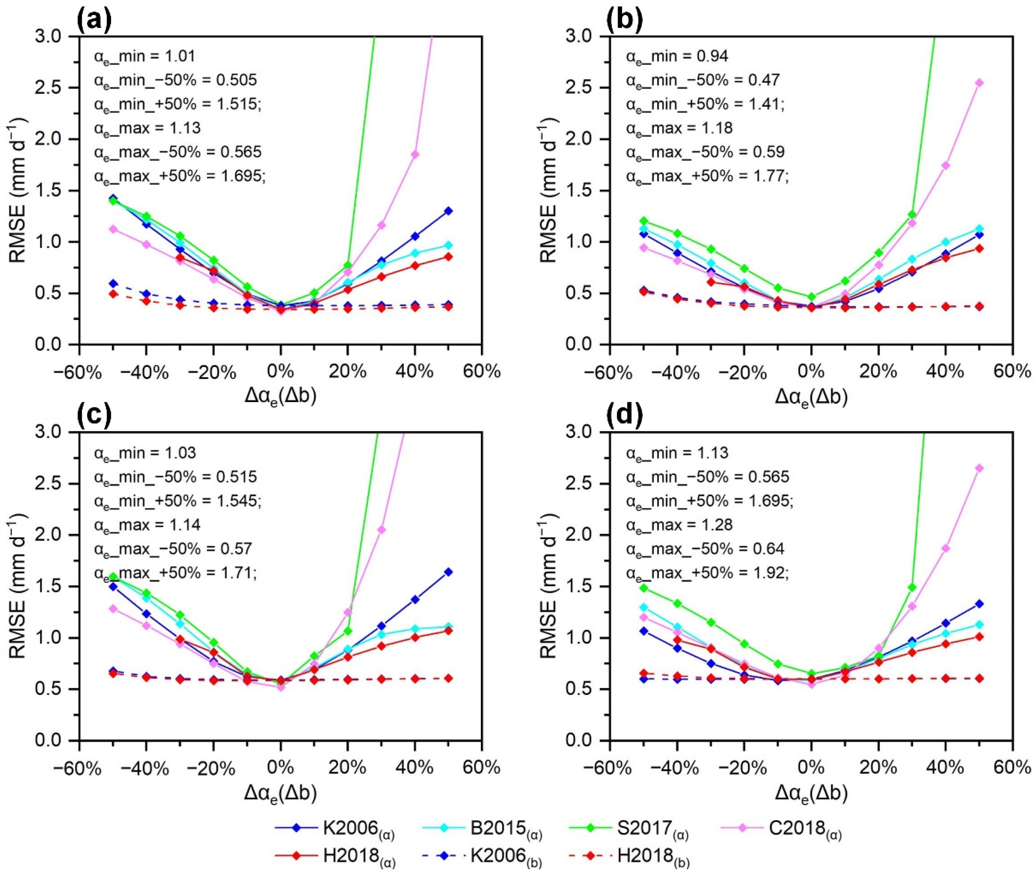
4.1.2. Sensitivity Analysis of CR-Based Models to Parameter Values

Then, we tested the sensitivity of five CR-based models to parameter values at each site, by adding increments from −50 to 50% at an interval of 10% to optimized parameter values for each CR-based model. Figure 8 displays the RMSE of the simulated E values for the in situ measurement. It is clear that variations in b values combined with constant αe values have little impact on evapotranspiration estimation, and a 50% variation in the αe value combined with constant b values led to increased RMSE values within 0.5 mm d−1. The K2006, B2015 and H2018 models exhibited lower sensitivity to variations in parameter values, and the H2018 model had the lowest sensitivity among all CR-based models.
We also noticed that larger RMSE values for the S2017 and C2018 models when the optimized αe value increased more than 20% because there were many abnormal E values, which indicated that the S2017 and C2018 models were more sensitive to parameter values, especially when the αe value increased more than 20%. Brutsaert [70] found that αe was closely related to the aridity index (AI, AI = Epa/P); accordingly, based on the global distribution of the parameter αe, the αe values were mainly from 0.8 to 1.2 around the world, except in extremely arid and wet regions. Assuming αe values were within the above scope in the present study–which means αe mainly varied from about −10% to 20% of its optimized values for all five CR models at each field site–according to Figure 8, the averaged RMSE increased by 0.14 mm d−1, 0.12 mm d−1, 0.15 mm d−1, 0.09 mm d−1 from the RMSE of the E estimated when using optimized αe values at TGL, XDT, BJ, and NAMORS, respectively.
Thus, the parameter αe value is very important to the accuracy of E estimation according to our study; certainly, the smaller deviation of optimized αe value would exert little impact on the accuracy of E estimation. Furthermore, the K2006 and H2018 models were completely insensitive to deviations of parameter b values.

4.2. Comparison with Previous Studies on the QTP at a Single Point Scale

Here, we compared estimation results of monthly E by five CR-based models in the present study with the latest two improved remote-sensing ET models that have been validated for the QTP. One is an improved MOD16 model by Yuan [71], referred to as “MOD16_Yuan” in this study; the another one is an improved SEBS model by Han [72], referred to as “SEBS_Han” in this study. Both obtained better accuracy with in situ measurements than that in previous results. Due to shared use observation data with Yuan’s work at NAMORS in 2009 and with Han’s work at BJ in 2013, the above two field sites during the corresponding period were chosen for comparison. Note that there are some differences in the observed E between this study and the above two works, which may be caused by different data procedure processes, such as quality control and gap-filling approaches.
Figure 9a exhibits the estimation results of monthly E by the CR approach and MOD16_Yuan model at NAMORS. Statistical results showed that in situ measured annual E values ranged from 467.2 to 481.6 mm, and the annual E values simulated from the five CR-based models were 495.5 mm (K2006), 455.6 mm (B2015), 371.1 mm (S2017), 418.4 mm (C2018), and 452.8 mm (H2018), respectively. For the MOD16_Yuan model, the annual E values reached 539.7 mm which was overestimated by 12.1% compared with in situ measurements. The largest bias occurred in June when the positive bias could reach 36 mm. The K2006 model overestimated the annual E by 6.1% with smaller positive deviations than the MOD16_Yuan model. The B2015 and H2018 models obtained better accuracy with smaller negative bias–approximately 20 mm on an annual scale–and both two CR-based models performed better than the K2006 and MOD16_Yuan models. However, the S2017 and C2018 models both performed poorly due to large negative biases, especially the S2017 model, with a bias of approximately 100 mm on an annual scale.
Figure 9b is the same as Figure 9a, but for BJ. Due to the lack of observed E data in some months, only available data during the corresponding month were analyzed. The simulated monthly E values by the five CR-based models were very close to each other– which could also capture the monthly variations in observed E–but a larger positive bias occurred in August. The SEBS_Han model performed well in August; however, it significantly overestimated monthly E values in May, June, and July, with a larger positive bias than that of the five CR-based models. Thus, the overall performance of the CR approach is still better than that of the SEBS_Han model in the present study.
Both the MOD16_Yuan and the SEBS_Han models have solid physical foundations, and the MOD16_Yuan model based on the original MOD16 model takes soil moisture and soil texture into soil evaporation estimation, and simultaneously optimizes canopy transpiration estimation. The SEBS_Han model introduces the description of the form drag caused by subgrid-scale topographical obstacles, the effective roughness lengths for momentum, and sensible heat transfer into the SEBS model. The above two models both improved the description capability of remote sensing models for the physical process of ET. For the CR approach, from another aspect of feedback of atmospheric evaporation demand to land surface moisture conditions, with a few unknown parameters and routine meteorological variables, the CR approach has also been demonstrated to have comparable accuracy with current sophisticated ET models in the present study.

4.3. Perspectives from the Present CR-Based Model Evaluations

This study provided a relatively comprehensive assessment about applicability of the CR-based models to frozen ground regions on the QTP. A performance comparison of five CR-based models was evaluated at four observation field sites. After local calibration, the E estimated by all five CR-based models captured daily variations; however, consistent with the findings of previous studies, it is difficult to capture daily variations during cold seasons (Figure 5). The reason for poor performance during cold seasons is still unclear. Theoretically, variable Epo (approximated by the Priestley-Taylor equation) in the CR approach assumes evaporation for an extensive saturation with minimal advection; however, during cold seasons, air advection is usually stronger than that in warm seasons. Thus, greater deviations may be derived from the conduction of Epo by only local air temperature and humidity in cold seasons, and the degree of land–atmosphere coupling during the cold season is usually weaker than that in warm seasons. The above conditions for cold seasons hardly satisfy the requirements of the CR approach.
Han [65] pointed out that accurate terrestrial ET estimation depends on precisely determining the land surface and atmospheric status; however, the deficiencies of CR-based models are focused only on the atmospheric status and neglect the land surface status, and the influence of land surface status on evaporation processes may not be fully captured through changes in atmospheric status alone, especially at small spatiotemporal scales. The CR principle may be an alternatively valuable approach when there is a lack of land surface information in the past, but for now, remote-sensing technologies make obtaining information on land surface status significantly easier. The CR approach also needs to take land surface information into account. Currently, some studies [70,73,74] have introduced shallow soil moisture, the vegetation index, or AI into the CR approach when applied at large-scale regions. Some other studies [75,76] also adhere to using only atmospheric status information, developing a free-calibrated CR approach when estimating large-scale ET. Further assessments about two different CR approaches need to be explored in the future.

5. Conclusions

This work assessed the actual evapotranspiration estimated by the CR approach in the frozen ground regions of the QTP. The uncertainties associated with observation and modeling of E at point scale were analyzed by investigating the parameter determined by different lengths of calibrated periods and parameter deviations on the accuracy of E estimation. Finally, two more latest works were compared with the CR-based models in this study at BJ and NAMORS.
Five CR-based models–whether with default or calibrated parameters–performed well in daily E estimation: the NSE values were both above 0.7, the accuracy of each CR-based model was close to another, the C2018 and H2018 models performed better among five CR-based models on daily and monthly timescales at four field sites, and the S2017 model performed poorest. The five CR-based models could estimate daily E during warm seasons, however, they are hardly applied during cold seasons. Nevertheless, the amount of E during cold seasons only account for small proportion of annual evaporation. Therefore, CR-based models with fewer data requirements and parameters provide a feasible approach to estimate daily and monthly E without needing detailed information on moisture and vegetation in the frozen ground regions of the QTP.
For calibrated parameter αe and b in CR-based models, all models are more sensitive to variations of αe than b. Specifically, within a certain range of deviations of parameter αe (for example, deviations from −10 to 30% in this study), the RMSE values will increase about 0.1 mm d−1 compared with RMSE of E estimation with optimized parameter values. Parameter b has little impact on the accuracy of E estimation. Thus, reasonable parameter αe values are of much importance to the performance of CR-based models.
Compared with previous studies about the application of CR-based models on the QTP, this study uses more in situ measurement data and more CR-based models. The present study also demonstrates better capability of CR approach on estimating E in high altitude and cold regions over QTP. At present, the CR approach has been developed as a benchmarking tool for large-scale evapotranspiration estimates, however, discrepancies in different spatiotemporal scales with other mainstream evapotranspiration products indicated that with the exception of developing physically CR-based models, hybrid modelling approaches such as combining CR approach with data-driven models are of great significance to large-scale and high-accuracy ET estimation in the future.

Author Contributions

C.S.: Formal analysis, Writing—original draft, Visualization. T.W. (Tonghua Wu): Conceptualization, Supervision, Writing—review & editing. N.M.: Conceptualization, Methodology, Writing—review & editing. J.W.: Conceptualization, Methodology, Writing—review & editing. X.L.: Writing—review & editing. X.Z.: Writing—review & editing. T.W. (Tianye Wang): Writing—review & editing. G.H.: Writing—review & editing. R.L.: Conceptualization. S.Y.: Conceptualization. J.C.: Conceptualization. J.Y.: Conceptualization. C.Y.: Writing—review & editing. All authors have read and agreed to the published version of the manuscript.

Funding

This research was funded by the National Natural Science Foundations of China (grant number 41771076, 41690142, 42001071), the West Light Foundation of Chinese Academy of Sciences (Tonghua Wu), the “Hundred Talents program” of Chinese Academy of Sciences (Sizhong Yang), the Open Research Fund Program of State Key Laboratory of Cryospheric Science, Northwest Institute of Eco-Environment and Resources, Chinese Academy of Sciences (grant number: SKLCSOP-2020-11). And The APC was funded by Tonghua Wu.

Data Availability Statement

The data that support the findings of this study are available from the corresponding author upon request (Tonghua Wu, [email protected]).

Acknowledgments

The authors would like to thank Xuelong Chen, Cunbo Han and Ling Yuan for sharing the original and modelling data at BJ and NAMORS.

Conflicts of Interest

The authors declare that they have no known competing financial interest or personal relationships that could have appeared to influence the work reported in this paper.

References

  1. Wang, K.; Dickinson, R.E. A review of global terrestrial evapotranspiration: Observation, modeling, climatology, and climatic variability. Rev. Geophys. 2012, 50, RG2005. [Google Scholar] [CrossRef]
  2. Jung, M.; Reichstein, M.; Ciais, P.; Seneviratne, S.I.; Sheffield, J.; Goulden, M.L.; Bonan, G.; Cescatti, A.; Chen, J.; Jeu, R.; et al. Recent decline in the global land evapotranspiration trend due to limited moisture supply. Nature 2010, 467, 951–954. [Google Scholar] [CrossRef]
  3. Fisher, J.B.; Melton, F.; Middleton, E.; Hain, C.; Anderson, M.; Allen, R.; McCabe, M.F.; Hook, S.; Baldocchi, D.; Townsend, P.A.; et al. The future of evapotranspiration: Global requirements for ecosystem functioning, carbon and climate feedbacks, agricultural management, and water resources. Water Resour. Res. 2017, 53, 2618–2626. [Google Scholar] [CrossRef]
  4. Anderson, M.C.; Allen, R.G.; Morse, A.; Kustas, W.P. Use of Landsat thermal imagery in monitoring evapotranspiration and managing water resources. Remote Sens. Environ. 2012, 122, 50–65. [Google Scholar] [CrossRef]
  5. Xiang, K.; Li, Y.; Horton, R.; Feng, H. Similarity and difference of potential evapotranspiration and reference crop evapotranspiration—A review. Agric. Water Manag. 2020, 232, 106043. [Google Scholar] [CrossRef]
  6. Allen, R.G.; Pereira, L.S.; Howell, T.A.; Jensen, M.E. Evapotranspiration information reporting: I. Factors governing measurement accuracy. Agric. Water Manag. 2011, 98, 899–920. [Google Scholar] [CrossRef] [Green Version]
  7. McMahon, T.A.; Peel, M.C.; Lowe, L.; Srikanthan, R.; McVicar, T.R. Estimating actual, potential, reference crop and pan evaporation using standard meteorological data: A pragmatic synthesis. Hydrol. Earth Syst. Sci. 2013, 17, 1331–1363. [Google Scholar] [CrossRef] [Green Version]
  8. Salvucci, G.D.; Gentine, P. Emergent relation between surface vapor conductance and relative humidity profiles yields evaporation rates from weather data. Proc. Natl. Acad. Sci. USA 2013, 110, 6287–6291. [Google Scholar] [CrossRef] [PubMed] [Green Version]
  9. Fisher, J.B.; Lee, B.; Purdy, A.J.; Halverson, G.H.; Dohlen, M.B.; Cawse-Nicholson, K.; Wang, A.; Anderson, R.G.; Aragon, B.; Arain, M.A.; et al. ECOSTRESS: NASA’s Next Generation Mission to Measure Evapotranspiration From the International Space Station. Water Resour. Res. 2020, 56, e2019WR026058. [Google Scholar] [CrossRef]
  10. Mueller, B.; Hirschi, M.; Jimenez, C.; Ciais, P.; Dirmeyer, P.A.; Dolman, A.J.; Fisher, J.B.; Jung, M.; Ludwig, F.; Maignan, F.; et al. Benchmark products for land evapotranspiration: LandFlux-EVAL multi-data set synthesis. Hydrol. Earth Syst. Sci. 2013, 17, 3707–3720. [Google Scholar] [CrossRef] [Green Version]
  11. Zhang, K.; Kimball, J.S.; Running, S.W. A review of remote sensing based actual evapotranspiration estimation. Wires. Water. 2016, 3, 834–853. [Google Scholar] [CrossRef]
  12. Jung, M.; Koirala, S.; Weber, U.; Ichii, K.; Gans, F.; Camps-Valls, G.; Papale, D.; Schwalm, C.; Tramontana, G.; Reichstein, M. The FLUXCOM ensemble of global land-atmosphere energy fluxes. Sci. Data 2019, 6, 74. [Google Scholar] [CrossRef] [Green Version]
  13. Fisher, J.B.; Tu, K.P.; Baldocchi, D.D. Global estimates of the land–atmosphere water flux based on monthly AVHRR and ISLSCP-II data, validated at 16 FLUXNET sites. Remote Sens. Environ. 2008, 112, 901–919. [Google Scholar] [CrossRef]
  14. Vinukollu, R.K.; Wood, E.F.; Ferguson, C.R.; Fisher, J.B. Global estimates of evapotranspiration for climate studies using multi-sensor remote sensing data: Evaluation of three process-based approaches. Remote Sens. Environ. 2011, 115, 801–823. [Google Scholar] [CrossRef]
  15. Wang, K.; Ma, N.; Zhang, Y.; Qiang, Y.; Guo, Y. Evapotranspiration and energy partitioning of a typical alpine wetland in the central Tibetan Plateau. Atmos. Res. 2022, 267, 105931. [Google Scholar] [CrossRef]
  16. Pan, S.; Pan, N.; Tian, H.; Friedlingstein, P.; Sitch, S.; Shi, H.; Arora, V.K.; Haverd, V.; Jain, A.K.; Kato, E.; et al. Evaluation of global terrestrial evapotranspiration using state-of-the-art approaches in remote sensing, machine learning and land surface modeling. Hydrol. Earth Syst. Sci. 2020, 24, 1485–1509. [Google Scholar] [CrossRef] [Green Version]
  17. Penman, H.L. Natural evaporation from open water, bare soil and grass. Proc. R. Soc. Lond. Ser. A—Math. Phys. Sci. 1948, 193, 120–145. [Google Scholar] [CrossRef] [Green Version]
  18. Monteith, J.L. Evaporation and Environment. 19th Symposia of the Society for Experimental Biology; University Press: Cambridge, UK, 1965; Volume 19, pp. 205–234. [Google Scholar]
  19. Ramírez, J.A.; Hobbins, M.T.; Brown, T.C. Observational evidence of the complementary relationship in regional evaporation lends strong support for Bouchet’s hypothesis. Geophys. Res. Lett. 2005, 32, L15401. [Google Scholar] [CrossRef] [Green Version]
  20. Han, S.; Tian, F.; Hu, H. Positive or negative correlation between actual and potential evaporation? Evaluating using a nonlinear complementary relationship model. Water Resour. Res. 2014, 50, 1322–1336. [Google Scholar] [CrossRef]
  21. Bouchet, R.J. Evapotranspiration reelle, evapotranspiration potentielle, et production agricole. Ann. Agron. 1963, 14, 743–824. [Google Scholar]
  22. Ma, N.; Zhang, Y.; Xu, C.Y.; Szilagyi, J. Modeling actual evapotranspiration with routine meteorological variables in the data-scarce region of the Tibetan Plateau: Comparisons and implications. J. Geophys. Res. Biogeosci. 2015, 120, 1638–1657. [Google Scholar] [CrossRef] [Green Version]
  23. Ma, N.; Szilagyi, J.; Zhang, Y.; Liu, W. Complementary-Relationship-Based Modeling of Terrestrial Evapotranspiration Across China During 1982–2012: Validations and Spatiotemporal Analyses. J. Geophys. Res. Atmos. 2019, 124, 4326–4351. [Google Scholar] [CrossRef]
  24. Han, S.; Tian, F. A review of the complementary principle of evaporation: From the original linear relationship to generalized nonlinear functions. Hydrol. Earth Syst. Sci. 2020, 24, 2269–2285. [Google Scholar] [CrossRef]
  25. Brutsaert, W.; Stricker, H. An advection-aridity approach to estimate actual regional evapotranspiration. Water Resour. Res. 1979, 15, 443–450. [Google Scholar] [CrossRef]
  26. Morton, F.I. Operational estimates of areal evapotranspiration and their significance to the science and practice of hydrology. J. Hydrol. 1983, 66, 1–76. [Google Scholar] [CrossRef]
  27. Granger, R.J.; Gray, D.M. Evaporation from natural nonsaturated surfaces. J. Hydrol. 1989, 111, 21–29. [Google Scholar] [CrossRef]
  28. Kahler, D.M.; Brutsaert, W. Complementary relationship between daily evaporation in the environment and pan evaporation. Water Resour. Res. 2006, 42, W05413. [Google Scholar] [CrossRef]
  29. Szilagyi, J. On the inherent asymmetric nature of the complementary relationship of evaporation. Geophys. Res. Lett. 2007, 34, L02405. [Google Scholar] [CrossRef] [Green Version]
  30. Han, S.; Hu, H.; Yang, D. A complementary relationship evaporation model referring to the Granger model and the advection-aridity. Hydrol. Process. 2011, 25, 2094–2101. [Google Scholar] [CrossRef]
  31. Han, S.; Hu, H.; Tian, F. A nonlinear function approach for the normalized complementary relationship evaporation model. Hydrol. Process. 2012, 26, 3973–3981. [Google Scholar] [CrossRef]
  32. Brutsaert, W. A generalized complementary principle with physical constraints for land-surface evaporation. Water Resour. Res. 2015, 51, 8087–8093. [Google Scholar] [CrossRef] [Green Version]
  33. Crago, R.; Szilagyi, J.; Qualls, R.; Huntington, J. Rescaling the complementary relationship for land surface evaporation. Water Resour. Res. 2016, 52, 8461–8471. [Google Scholar] [CrossRef]
  34. Crago, R.D.; Qualls, R.J. Evaluation of the Generalized and Rescaled Complementary Evaporation Relationships. Water Resour. Res. 2018, 54, 8086–8102. [Google Scholar] [CrossRef]
  35. Szilagyi, J.; Crago, R.; Qualls, R. A calibration-free formulation of the complementary relationship of evaporation for continental-scale hydrology. J. Geophys. Res. Atmos. 2017, 122, 264–278. [Google Scholar] [CrossRef]
  36. Han, S.; Tian, F. Derivation of a Sigmoid Generalized Complementary Function for Evaporation With Physical Constraints. Water Resour. Res. 2018, 54, 5050–5068. [Google Scholar] [CrossRef]
  37. Gao, B.; Xu, X. Derivation of an exponential complementary function with physical constraints for land surface evaporation estimation. J. Hydrol. 2021, 593, 125623. [Google Scholar] [CrossRef]
  38. Crago, R.; Crowley, R. Complementary relationships for near-instantaneous evaporation. J. Hydrol. 2005, 300, 199–211. [Google Scholar] [CrossRef]
  39. Huntington, J.L.; Szilagyi, J.; Tyler, S.W.; Pohll, G.M. Evaluating the complementary relationship for estimating evapotranspiration from arid shrublands. Water Resour. Res. 2011, 47, W05533. [Google Scholar] [CrossRef] [Green Version]
  40. Xu, X.; Li, X.; Wang, X.; He, C.; Tian, W.; Tian, J.; Yang, L. Estimating daily evapotranspiration in the agricultural-pastoral ecotone in Northwest China: A comparative analysis of the Complementary Relationship, WRF-CLM4.0, and WRF-Noah methods. Sci. Total Environ. 2020, 729, 138635. [Google Scholar] [CrossRef]
  41. Zhou, H.; Han, S.; Liu, W. Evaluation of two generalized complementary functions for annual evaporation estimation on the Loess Plateau, China. J. Hydrol. 2020, 587, 124980. [Google Scholar] [CrossRef]
  42. Wang, L.; Han, S.; Tian, F. At which timescale does the complementary principle perform best in evaporation estimation? Hydrol. Earth Syst. Sci. 2021, 25, 375–386. [Google Scholar] [CrossRef]
  43. Qiu, J. China: The third pole. Nature 2008, 454, 393–396. [Google Scholar] [CrossRef] [PubMed] [Green Version]
  44. Duan, A.M.; Wu, G.X.; Liu, Y.M.; Ma, Y.M.; Zhao, P. Weather and climate effects of the Tibetan Plateau. Adv. Atmos. Sci. 2012, 29, 978–992. [Google Scholar] [CrossRef]
  45. Wu, G.; Duan, A.; Liu, Y.; Mao, J.; Ren, R.; Bao, Q.; He, B.; Liu, B.; Hu, W. Tibetan Plateau climate dynamics: Recent research progress and outlook. Natl. Sci. Rev. 2015, 2, 100–116. [Google Scholar] [CrossRef] [Green Version]
  46. Zou, D.; Zhao, L.; Sheng, Y.; Chen, J.; Hu, G.; Wu, T.; Wu, J.; Xie, C.; Wu, X.; Pang, Q.; et al. A new map of permafrost distribution on the tibetan plateau. Cryosphere 2017, 11, 2527–2542. [Google Scholar] [CrossRef] [Green Version]
  47. Cheng, G.; Wu, T. Responses of permafrost to climate change and their environmental significance, Qinghai-Tibet Plateau. J. Geophys. Res. Earth. 2007, 112, F02S03. [Google Scholar] [CrossRef] [Green Version]
  48. Zhao, L.; Zou, D.; Hu, G.; Du, E.; Pang, Q.; Xiao, Y.; Li, R.; Sheng, Y.; Wu, X.; Sun, Z.; et al. Changing climate and the permafrost environment on the Qinghai–Tibet (Xizang) plateau. Permafrost. Periglac. 2020, 31, 396–405. [Google Scholar] [CrossRef]
  49. Ma, Y.; Kang, S.; Zhu, L.; Xu, B.; Tian, L.; Yao, T. ROOF OF THE WORLD: Tibetan Observation and Research Platform. Bull. Am. Meteorol. Soc. 2008, 89, 1487–1492. [Google Scholar] [CrossRef] [Green Version]
  50. Ma, Y.; Ma, W.; Zhong, L.; Hu, Z.; Li, M.; Zhu, Z.; Han, C.; Wang, B.; Liu, X. Monitoring and Modeling the Tibetan Plateau’s climate system and its impact on East Asia. Sci. Rep. 2017, 7, 44574. [Google Scholar] [CrossRef] [PubMed] [Green Version]
  51. Wang, G.; Lin, S.; Hu, Z.; Lu, Y.; Sun, X.; Huang, K. Improving Actual Evapotranspiration Estimation Integrating Energy Consumption for Ice Phase Change Across the Tibetan Plateau. J. Geophys. Res. Atmos. 2020, 125, e2019JD031799. [Google Scholar] [CrossRef]
  52. Zhao, L.; Zou, D.; Hu, G.; Wu, T.; Du, E.; Liu, G.; Xiao, Y.; Li, R.; Pang, Q.; Qiao, Y.; et al. A synthesis dataset of permafrost thermal state for the Qinghai–Tibet (Xizang) Plateau, China. Earth Syst. Sci. Data 2021, 13, 4207–4218. [Google Scholar] [CrossRef]
  53. Ma, Y.; Hu, Z.; Xie, Z.; Ma, W.; Wang, B.; Chen, X.; Li, M.; Zhong, L.; Sun, F.; Gu, L.; et al. A long-term (2005–2016) dataset of hourly integrated land-atmosphere interaction observations on the Tibetan Plateau. Earth Syst. Sci. Data 2020, 12, 2937–2957. [Google Scholar] [CrossRef]
  54. Liu, S.M.; Xu, Z.W.; Wang, W.Z.; Jia, Z.Z.; Zhu, M.J.; Bai, J.; Wang, J.M. A comparison of eddy-covariance and large aperture scintillometer measurements with respect to the energy balance closure problem. Hydrol. Earth Syst. Sci. 2011, 15, 1291–1306. [Google Scholar] [CrossRef] [Green Version]
  55. You, Q.; Xue, X.; Peng, F.; Dong, S.; Gao, Y. Surface water and heat exchange comparison between alpine meadow and bare land in a permafrost region of the Tibetan Plateau. Agric. For. Meteorol. 2017, 232, 48–65. [Google Scholar] [CrossRef]
  56. Gu, L.; Yao, J.; Hu, Z.; Zhao, L. Comparison of the surface energy budget between regions of seasonally frozen ground and permafrost on the Tibetan Plateau. Atmos. Res. 2015, 153, 553–564. [Google Scholar] [CrossRef]
  57. Yang, K.; Wang, J. A temperature prediction-correction method for estimating surface soil heat flux from soil temperature and moisture data. Sci. China. Ser. D Earth Sci. 2008, 51, 721–729. [Google Scholar] [CrossRef]
  58. Yao, J.; Zhao, L.; Gu, L.; Qiao, Y.; Jiao, K. The surface energy budget in the permafrost region of the Tibetan Plateau. Atmos. Res. 2011, 102, 394–407. [Google Scholar] [CrossRef]
  59. Ma, N.; Zhang, Y.; Guo, Y.; Gao, H.; Zhang, H.; Wang, Y. Environmental and biophysical controls on the evapotranspiration over the highest alpine steppe. J. Hydrol. 2015, 529, 980–992. [Google Scholar] [CrossRef]
  60. Parlange, M.B.; Katul, G.G. An Advection-Aridity evaporation model. Water Resour. Res. 1992, 28, 127–132. [Google Scholar] [CrossRef]
  61. Szilagyi, J.; Jozsa, J. New findings about the complementary relationship-based evaporation estimation methods. J. Hydrol. 2008, 354, 171–186. [Google Scholar] [CrossRef] [Green Version]
  62. Szilagyi, J. Temperature corrections in the Priestley–Taylor equation of evaporation. J. Hydrol. 2014, 519, 455–464. [Google Scholar] [CrossRef]
  63. Dai, L.; Fu, R.; Guo, X.; Ke, X.; Du, Y.; Zhang, F.; Li, Y.; Qian, D.; Zhou, H.; Cao, G. Evaluation of actual evapotranspiration measured by large-scale weighing lysimeters in a humid alpine meadow, northeastern Qinghai-Tibetan Plateau. Hydrol. Process. 2021, 35, e14051. [Google Scholar] [CrossRef]
  64. Wang, L.; Tian, F.; Han, S.; Wei, Z. Determinants of the Asymmetric Parameter in the Generalized Complementary Principle of Evaporation. Water Resour. Res. 2020, 56, e2019WR026570. [Google Scholar] [CrossRef]
  65. Han, S.; Tian, F. Research Progress of the Generalized Nonlinear Complementary Relationships of Evaporation. Adv. Earth Sci. 2021, 36, 849–861, (In Chinese with English Abstract). [Google Scholar]
  66. Gan, G.; Liu, Y.; Chen, D.; Zheng, C. Investigation of a non-linear complementary relationship model for monthly evapotranspiration estimation at global flux sites. J. Hydrometeorol. 2021, 22, 2645–2658. [Google Scholar] [CrossRef]
  67. Szilagyi, J.; Crago, R.D. Comment on “Derivation of a Sigmoid Generalized Complementary Function for Evaporation With Physical Constraints” by S. Han and F. Tian. Water Resour. Res. 2019, 55, 868–869. [Google Scholar] [CrossRef]
  68. Crago, R.D.; Szilagyi, J.; Qualls, R. Comment on: “A review of the complementary principle of evaporation: From the original linear relationship to generalized nonlinear functions” by Han and Tian (2020). Hydrol. Earth Syst. Sci. 2021, 25, 63–68. [Google Scholar] [CrossRef]
  69. Ma, N.; Zhang, Y.; Szilagyi, J.; Guo, Y.; Zhai, J.; Gao, H. Evaluating the complementary relationship of evapotranspiration in the alpine steppe of the Tibetan Plateau. Water Resour. Res. 2015, 51, 1069–1083. [Google Scholar] [CrossRef] [Green Version]
  70. Brutsaert, W.; Cheng, L.; Zhang, L. Spatial Distribution of Global Landscape Evaporation in the Early Twenty-First Century by Means of a Generalized Complementary Approach. J. Hydrometeorol. 2020, 21, 287–298. [Google Scholar] [CrossRef]
  71. Yuan, L.; Ma, Y.; Chen, X.; Wang, Y.; Li, Z. An Enhanced MOD16 Evapotranspiration Model for the Tibetan Plateau During the Unfrozen Season. J. Geophys. Res. Atmos. 2021, 126, e2020JD032787. [Google Scholar] [CrossRef]
  72. Han, C.; Ma, Y.; Wang, B.; Zhong, L.; Ma, W.; Chen, X.; Su, Z. Long-term variations in actual evapotranspiration over the Tibetan Plateau. Earth Syst. Sci. Data 2021, 13, 3513–3524. [Google Scholar] [CrossRef]
  73. Zhang, L.; Brutsaert, W. Blending the Evaporation Precipitation Ratio With the Complementary Principle Function for the Prediction of Evaporation. Water Resour. Res. 2021, 57, e2021WR029729. [Google Scholar] [CrossRef]
  74. Zhou, H.; Li, Z.; Liu, W. Connotation analysis of parameters in the generalized nonlinear advection aridity model. Agric. For. Meteorol. 2021, 301, 108343. [Google Scholar] [CrossRef]
  75. Szilagyi, J.; Crago, R.; Ma, N. Dynamic Scaling of the Generalized Complementary Relationship Improves Long-term Tendency Estimates in Land Evaporation. Adv. Atmos. Sci. 2020, 37, 975–986. [Google Scholar] [CrossRef]
  76. Ma, N.; Szilagyi, J. The CR of Evaporation: A Calibration-Free Diagnostic and Benchmarking Tool for Large-Scale Terrestrial Evapotranspiration Modeling. Water Resour. Res. 2019, 55, 7246–7274. [Google Scholar] [CrossRef] [Green Version]
Figure 1. Locations of four observation field sites on the QTP.
Remotesensing 14 02047 g001
Figure 2. Comparison of available energy (RnG) and sum of turbulent fluxes (H + LE) for the daily-averaged measurements after gap-filled during study period at four selected sites: (a) TGL; (b) XDT; (c) BJ; (d) NAMORS. The black solid line is the 1:1 line, and the black dash line fitted by the linear regression.
Remotesensing 14 02047 g002
Figure 3. The daily variations of E (blue circles), sublimation (red circles), Erad (pink line), and Epa (gray area) during the study period at the observation fields: (a) TGL; (b) XDT; (c) BJ; (d) NAMORS. “W” represents warm season and “C” represents cold season.
Remotesensing 14 02047 g003
Figure 4. Comparison of simulated daily actual evapotranspiration (Esim) rates by five CR-based models with default parameter against measurements made using EC system at (ae) TGL; (fj) XDT; (ko) BJ; (pt) NAMORS, respectively. The blue scattered dots and dash lines represent E estimated by default parameter values and its fitting line; the red scattered dots and dash lines represent E estimated by calibrated parameter values and its fitting line; the black solid line is the 1:1 line.
Remotesensing 14 02047 g004
Figure 5. Scatter plot of y versus different rescaling x for five CR-based functions at four observation sites (dots, at), blue scattered dots represent data during cold season and red scattered dots represent data during warm season, green scattered dots represent data that could not meet the preconditions of CR approach. The solid lines fitted by CR-based functions with calibrated parameter values.
Remotesensing 14 02047 g005
Figure 6. Comparison of monthly E values estimated by five CR functions with calibrated parameters against measurements by eddy-covariance system at (a) TGL; (b) XDT; (c) BJ; (d) NAMORS, respectively. Number in parentheses are available days during corresponding month.
Remotesensing 14 02047 g006
Figure 7. Bias of monthly E estimated by five CR-based models at (ae) TGL; (fj) XDT; (ko) BJ; (pt) NAMORS, respectively. Dash lines represent annual total bias. The grey filled area represents the warm season.
Remotesensing 14 02047 g007
Figure 8. Sensitivity analysis of CR-based models to the parameter αe and b at (a) TGL, (b) XDT, (c) BJ, and (d) NAMORS. Δαe represents the increment to the optimized αe values for all five CR-based models and Δb represents the increment to the optimized b values for K2006 and H2018 model. Suffix “(α)” and “(b)” represents simulated actual ET with perturbations of α (with constant b) and b (with constant α), respectively.
Remotesensing 14 02047 g008
Figure 9. Comparison of monthly observed E values (filled area enclosed by calculated results from this study and another corresponding work) and simulated E values (solid lines) of CR-based models with improved MOD16 evapotranspiration model by Yuan [71] at (a) NAMORS; with improved SEBS model by Han [72] at (b) BJ.
Remotesensing 14 02047 g009
Table 1. Sum of daily rainfall (mm), E plus sublimation (mm), Epa (mm) for two periods of every observational year. The warm season is from May to September, the cold season is from January to April and October to December.
SitesVariablesFirst YearSecond Year
Warm SeasonCold SeasonAnnualWarm SeasonCold SeasonAnnual
TGLRainfall339.554.3393.8355.936391.9
(N1 = 365;E plus Sublimation362.170.9433364.781.6446.3
N2 = 360)Epa537.5409.7947.2496391.1887.1
XDTRainfall299.365.1364.4200.67207.6
(N1 = 363;E plus Sublimation312.482.9395.317824.4202.4
N2 = 185)Epa515.9410.1926309.7141.9451.6
BJRainfall a---38683.2469.2
(N1 = 363;E plus Sublimation432.9118.9551.8385.5117.3502.8
N2 = 350)Epa580.8421.51002.3549.8363.4913.2
NAMORSRainfall b494.754.2548.932747.3374.3
(N1 = 337;E plus Sublimation413.6128.9542.5346121.2467.2
N2 = 352)Epa493.1336.1829.2531.6411.4943
Note: N1 represents available samples of first observational year, N2 represents available samples of second observational year. a Rainfall data on second year from Naqu country meteorological station; b Rainfall data on second year from Dangxiong country meteorological station.
Table 2. Statistical results of CR-based models with default and calibrated (in parentheses) parameter values against daily actual evapotranspiration measurements from four observation sites. Bold font indicates the best model based on maximum NSE values among five CR-based models.
SitesModelαebcRMSE
(mm d−1)
MAE
(mm d−1)
MBE
(mm d−1)
NSER2Average
(mm d−1)
TGLK20060.88 (1.01)16.67 (2.41)-0.457 (0.381)0.375 (0.31)0.053 (−0.056)0.84 (0.889)0.872 (0.891)1.24
B20150.92 (1.03)-−1.35 (2.22)0.428 (0.347)0.338 (0.269)0.109 (−0.032)0.86 (0.908)0.88 (0.91)
S20171.12 (1.13)--0.394 (0.388)0.279 (0.275)−0.136 (−0.112)0.881 (0.885)0.897 (0.899)
C20181.12 (1.08)--0.321 (0.324)0.244 (0.245)0.039 (−0.041)0.921 (0.919)0.924 (0.924)
H20180.97 (1.07)5.56 (1.44)-0.415 (0.343)0.328 (0.266)0.128 (−0.01)0.868 (0.91)0.889 (0.91)
XDTK20060.88 (0.94)16.67 (4.1)-0.372 (0.375)0.282 (0.281)0.052 (−0.07)0.839 (0.837)0.845 (0.852)1.09
B20150.92 (1.01)-−1.35 (1.48)0.388 (0.361)0.287 (0.268)0.093 (−0.049)0.826 (0.849)0.852 (0.861)
S20171.12 (1.18)--0.486 (0.467)0.354 (0.341)−0.198 (−0.07)0.725 (0.746)0.778 (0.799)
C20181.12 (1.11)--0.37 (0.366)0.277 (0.274)0.017 (−3.4 × 10⁻⁴)0.841 (0.844)0.852 (0.852)
H20180.97 (1.04)5.56 (1.8)-0.381 (0.36)0.289 (0.269)0.105 (−0.042)0.831 (0.849)0.856 (0.859)
BJK20060.88 (1.03)16.67 (2.63)-0.609 (0.59)0.463 (0.439)0.001 (0.003)0.746 (0.762)0.748 (0.773)1.44
B20150.92 (1.05)-−1.35 (2.55)0.604 (0.578)0.453 (0.42)0.074 (−0.031)0.75 (0.772)0.755 (0.789)
S20171.12 (1.14)--0.544 (0.553)0.405 (0.41)−0.156 (−0.092)0.798 (0.791)0.826 (0.824)
C20181.12 (1.11)--0.531 (0.523)0.377 (0.371)0.038 (0.013)0.808 (0.813)0.819 (0.821)
H20180.97 (1.11)5.56 (1.17)-0.596 (0.584)0.45 (0.421)0.092 (−0.013)0.757 (0.767)0.764 (0.792)
NAMORSK20060.88 (1.13)16.67 (10.07)-0.637 (0.601)0.458 (0.464)−0.231 (0.08)0.704 (0.737)0.755 (0.757)1.33
B20150.92 (1.17)-−1.35 (0.76)0.607 (0.585)0.448 (0.455)−0.204 (−0.033)0.731 (0.751)0.764 (0.774)
S20171.12 (1.25)--0.756 (0.653)0.573 (0.516)−0.516 (−0.273)0.583 (0.689)0.78 (0.785)
C20181.12 (1.2)--0.579 (0.549)0.422 (0.413)−0.264 (−0.139)0.756 (0.78)0.806 (0.803)
H20180.97 (1.28)5.56 (1.72)-0.601 (0.6)0.431 (0.475)−0.197 (−0.041)0.737 (0.738)0.769 (0.776)
Table 3. Bias of simulated E by CR-based models with calibrated parameter values against measurements by EC on different timescales (monthly, seasonal, annual) at TGL, XDT, BJ and NAMORS. Grey-filled area is warm season period (May to September), bold font stands for model with minimum absolute bias during corresponding period.
SiteModelJanFebMarAprMayJunJulAugSepOctNovDecWarm SeasonCold SeasonYear
TGLK20060.06413.0714.844.91−4.75−9.91−9.49−8.03−10.39−9.12−5.21−27.277.25−20.02
B20151.654.4912.0112.544.18−2.86−7.55−7.9−7.44−11.54−8.36−0.59−21.5710.2−11.37
S20170.220.23.351.15−0.320.69−3.77−7.25−6.33−15.3−10.06−2.86−16.98−23.3−40.28
C20182.234.289.028.333.09−2.08−7.31−8.68−6.21−9.51−7−0.8−21.196.55−14.64
H20181.945.1212.3812.614.51−1.67−6.21−6.76−6.72−11.41−7.850.316.8513.093.76
XDTK2006−2.54−3.191.47-1.122.48−4.26−0.27−0.52-−3.41−3.77−1.45−11.44−12.89
B2015−1.68−3.061.02-−0.372.82−3.921.810.88-−3.07−3.421.22−10.21−8.99
S2017−3.4−5.35−0.52-−4.282.02−5.425.85.67-−3.29−4.23.79−16.76−12.97
C2018−0.28−1.551.19-−0.613.76−5.013.933.9-−2.52−2.875.976.030.06
H2018−1.15−2.541.17-−0.652.66−4.041.871.05-−2.99−3.230.89−8.74−7.85
BJK2006−3.07−0.88.0610.73−1.254.63−11.7214.75−5.06−5.56−6.92−2.661.350.221.13
B2015−3.13−1.775.085.79−3.94.11−9.1114.12−4.22−6.35−9.28−2.251−11.91−10.91
S2017−5.14−4.91−0.5−0.89−7.310.89−2.9310.88−0.86−6.06−11.33−3.980.67−32.81−32.14
C2018−2.660.254.028.24−2.223.27−6.7213.17−1.86−4.37−6.23−0.485.64−1.234.41
H2018−2.99−1.924.544.86−3.485.65−6.5515.5−2.68−5.9−9.49−2.218.44−13.11−4.67
NAMORSK2006−7.920.736.1722.7118.6715.865.41−18−2.06−2.72−5.96−4.5919.888.4228.3
B2015−10.5−3.521.715.6214.6312.233.11−16.32−6.57−8.49−8.37−5.127.08−18.6811.6
S2017−13.01−8.75−4.44−2.772.540.67−3.92−15.14−16.21−17.58−11.14−6.4−32.06−64.09−96.15
C2018−10.07−4.580.086.638.455.21−1.21−19.3−10.15−11.23−8.03−4.66−17−31.86−48.86
H2018−11.56−5.130.7714.3915.4513.34.75−15.05−6.28−9.85−9.5−5.712.17−26.58−14.41
Table 4. Comparison of simulated results by different CR-based models using two different calibrated parameter values during the warm season. One is calibrated by a whole year period, another is calibrated by a corresponding warm season.
SiteModelCalibrated Period by Warm SeasonCalibrated Period by Whole Year
αebcNSEαebcNSE
TGLK20061.022.49-0.7591.012.41-0.73
B20151-0.80.7641.03-2.220.752
S20171.12--0.5591.13--0.581
C20181.08--0.7311.08--0.731
H20181.012.58-0.7641.071.44-0.762
XDTK200612.93-0.6570.944.1-0.669
B20150.98-0.380.6561.01-1.480.657
S20171.18--0.3761.18--0.376
C20181.12--0.6071.11--0.617
H20180.993.03-0.6571.041.8-0.65
BJK20061.111.13-0.3231.032.63-0.357
B20151.1-4.660.2941.05-2.550.361
S20171.14--0.4291.14--0.429
C20181.11--0.4661.11--0.466
H20181.170.75-0.271.111.17-0.341
NAMORSK20061.183.81-0.5771.1310.07-0.58
B20151.19-1.010.5771.17-0.760.588
S20171.25--0.4921.25--0.492
C20181.2--0.6221.2--0.622
H20181.351.03-0.5251.281.72-0.573
Publisher’s Note: MDPI stays neutral with regard to jurisdictional claims in published maps and institutional affiliations.

