An Error Overbounding Method Based on a Gaussian Mixture Model with Uncertainty Estimation for a Dual-Frequency Ground-Based Augmentation System

Abstract

To ensure the integrity of a ground-based augmentation system (GBAS), an ionosphere-free (Ifree) filtering algorithm with dual-frequency measurements is employed to make the GBAS free of the first-order ionospheric influence. However, the Ifree algorithm outputs the errors of two frequencies. The protection level obtained via the traditional Gaussian overbound is overconservative. This conservatism may cause false alarms and diminish availability. An overbounding framework based on a Gaussian mixture model (GMM) is proposed to handle samples drawn from Ifree-based GBAS range errors. The GMM is employed to model the single-frequency errors that concern the uncertainty estimation. A Monte Carlo simulation is performed to determine the accuracy of the estimated GMM confidence level obtained by using the general estimation approach. Then, the final GMM used to overbound the Ifree error distribution is analyzed. Based on the convolution invariance property, vertical protection levels in the position domain are explicitly derived without introducing complex numerical calculations. A performance evaluation based on a real-world road test shows that the Ifree-based vertical protection levels are tightened with a small computational cost.

1. Introduction

The global positioning system (GPS), BeiDou navigation satellite system (BDS), Russian global navigation satellite system (GLONASS) and Galileo navigation satellite system are the four types of global navigation satellite systems (GNSSs) [1,2,3]. Based on a differential GNSS structure, a ground-based augmentation system (GBAS) can broadcast differential corrections to improve positioning accuracy and provide integrity, continuity, and availability for civil aircraft during their approaching and landing phases [4]. Among these four criteria, integrity is the key performance criterion for measuring the trust placed in the correctness of the provided navigation information [5]. Integrity refers to the ability to effectively provide warnings to users when system faults cause risks and jeopardize user safety.

The ionospheric anomaly is one of the most challenging issues in GBAS development [6]. Extreme ionospheric anomalies cause large differential errors, therefore leading to the loss of integrity. In single-frequency GBASs, authorized users are equipped with customized monitors to detect ionospheric anomalies [7]. Further, an auto-covariance estimation of variable samples (ACVES) algorithm can be an outstanding auxiliary to monitor ionospheric variations and disturbances [8]. However, the detection of severe ionospheric anomalies before users are threatened cannot be guaranteed [9]. Therefore, a single-frequency GBAS cannot provide high-level service under anomalous ionospheric conditions.

With regard to incoming GNSS signals, a GBAS approach service type (GAST) F based on multiconstellation and dual-frequency measurements has been proposed to support high-level precision approach operations [10]. GAST-F employs dual-frequency filtering algorithms to liberate the associated system from ionospheric anomalies. Two widely used filtering algorithms, which include the divergence-free (Dfree) and ionosphere-free (Ifree) filtering algorithms, are considered the primary choices [11]. The Dfree filtering algorithm utilizes single-frequency code measurements and dual-frequency phase measurements for smoothing. Despite the removal of the temporal ionospheric gradient, the Dfree filtering algorithm can provide more accurate performance. In contrast, the Ifree filtering algorithm uses dual-frequency code and phase measurements to remove all the first-order ionosphere-related items. The ionospheric anomalies are basically alleviated. A dual-frequency GBAS adopting the Ifree filtering algorithm is hereafter named an Ifree-based GBAS [9]. A high level of noise is induced because of the combination of the single-frequency errors, which is the main shortcoming of the Ifree-based GBAS.

When no fault or anomaly occurs, the GBAS ensures integrity by adopting a quintessentially conservative method named overbounds [12]. The GBAS replaces the distribution of the input real-world errors with conservative parametric models. Specifically, conservatism can be guaranteed because the accumulated tail probability of the overbound exceeds that of the input distribution. This conservatism can be delivered through a linear system to the output error models. All quantiles of the output errors are larger than those of the true errors for any integrity risk under fault-free conditions. The quantile corresponding to the integrity risk is also known as the protection level, which is a crucial test statistic for ensuring the integrity of the GBAS.

The actual distribution of the experimental GBAS errors presents heavier tails than those of a Gaussian distribution [13]. A Gaussian distribution whose variance is inflated to ensure that the tails of the actual errors are covered is named the Gaussian overbound. The Gaussian distribution is often utilized in augmentation systems [14]. However, the core of the Gaussian overbound is much larger than that of the actual error distribution. Therefore, protection levels based on the Gaussian overbound are loose and overconservative, resulting in a potential decline in system availability [15]. To address this issue, many complex distribution models have been employed to fit the underlying distributions of GBAS errors. However, these distributions may introduce an unignorable computational load to the airborne subsystem of the GBAS. Facilitating the computational process while maintaining a tight overbound is crucial for the future GBASs.

Protection levels need to be calculated for each epoch. As GAST-F is in its initial phase, the design of the overbound needs to be revisited to guarantee a better balance between integrity and availability in a dual-frequency GBAS. Ifree-based errors are a linear combination of single-frequency errors. The probability density function (PDF) of Ifree-based errors is the convolution of the two single-frequency error PDFs. Because the convolution operation is a weighted sum taken after sliding the PDFs of two frequency errors, the conservative core affects the tight tail parts and causes excessive amplification of the protection levels. If the Gaussian overbound is utilized, the Ifree filtering algorithm increases the protection levels by 2.6 or more when receiving measurements on the L1 and L5 signals of GPS [9]. Consequently, the Ifree-based protection level is too large to attain high availability. The achieved availability in the fault-free hypothesis may be reduced by over 80%, thereby restricting the practical application of GAST-F [16]. Nevertheless, little attention has been paid to this issue. A tight overbound resulting in a tight protection level is beneficial for enabling high availability. It is desirable to establish a framework for overbounding Ifree-based errors in a compact manner.

In this paper, a framework for overbounding Ifree-based errors is proposed. Basically, the errors of each frequency are overbounded. To accurately characterize heavy-tailed errors, a Gaussian mixture model (GMM) is utilized to overbound the single-frequency errors. GMMs have been used in the GNSS community [17], as they have the potential to alleviate the performance degradation caused by the conflicts between the Gaussian hypothesis and heavy-tailed distributions. To tighten the overbound, the GMM overbound is redesigned based on the uncertainty estimation to reduce its conservatism; this technique has not yet been considered. Therefore, to determine whether the parameter uncertainty estimation of the GMM is accurate, the confidence interval estimation accuracy is evaluated through theoretical analyses and simulation experiments. An overbound for Ifree-based errors is established by combining two single-frequency overbounds. Then, both the single-frequency and Ifree-based protection levels are derived by using the GMM overbound; this step is expected to optimize the system availability without significantly increasing the computational load. Therefore, tightened protection levels are likely to be calculated without inducing much additional computational cost.

This paper is organized as follows. Section 2 analyzes the succinct background concerning GBAS overbounding for single-frequency GBASs, with a focus on GMM overbounds. Section 3 outlines the details of the proposed overbounding method for dual-frequency GBASs, followed by derivations of the protection levels. Subsequently, our road-test setup is introduced in Section 4, and the experimental results are shown. A discussion follows in Section 5. Finally, the conclusions and contributions, as well as future work, are presented in Section 6.

2. Background

2.1. Previous Work on Single-Frequency Overbounds

For single-frequency augmentation systems, several excellent studies on the overbound of the independent errors include the CDF overbound [14,15,18], paired overbound [19,20], position-domain monitor [21,22,23] and two-step overbound [24]. Among all these approaches, the CDF overbound is the only one that is adopted in the standard GBAS. It is suitable for the ideal case in which zero-mean, unimodal, and symmetric errors are present. Such strict requirement shape requirements are the premise of well-behaved overbounds. The CDF overbound is defined as in [18].

$$\begin{array}{cc}{F}_{OB}\left(x\right)\le F\left(x\right)& \forall x\le 0\\ F_{OB}\left(x\right)>F\left(x\right)& \forall x>0\end{array}$$

(1)

where x is a random variable. F(x) is the underlying but unknown CDF of the random variable x. F_OB(x) is the overbounding CDF.

The offline-online CDF overbounding framework includes the establishment of a range error distribution model (REDM), the establishment of a range error overbounding model (REOM) and the calculation of the protection level. More details can be found in [15]. The first two steps are completed offline in the range domain of the ground subsystem by broadcasting conservative parameters that are valid for all satellites. Real-time processing is not required in either step. The last step is performed online in the airborne subsystem to calculate time-varying protection levels, which requires a high degree of timeliness.

Due to its simplicity and convolution invariance, an REOM in the form of a Gaussian distribution, namely, a Gaussian overbound, is recommended as a practical implementation. The specific implementation, including a Gaussian overbound utilizing a Gaussian-core exponential-tail (GCET) distribution and extreme value theory (EVT), can be found in [14,25]. Nevertheless, in the Gaussian distribution, only a standard derivation parameter can be adjusted. To ensure that the tails are overbounded, the standard derivation needs to be inflated. Inflation always makes the core larger than that of the actual distribution, leading to a loose overbound. A Gaussian overbound simply overbounds the underlying distribution to a certain probability and masks the underlying trend of the REDM. Countermeasures are adopted to guarantee a tighter overbound by using non-Gaussian overbounds that make the REOM less conservative. Non-Gaussian methods lead to tight overbounds, revealing the trend of the entire underlying distribution. At present, instances of such approaches include the stable overbound [26] and the Gaussian-Pareto overbound (GPO) [27]. Unfortunately, these two methods have defects in their mathematical properties. A main shortcoming of the stable overbound is its infinite second order [28]. The estimates of this overbound have the potential to diverge as the sample size increases. A major disadvantage of the GPO lies in the numerical calculation during the projection process, which cannot meet the requirements of real-time processing.

From the above analysis, two issues need to be solved. On the one hand, the existing overbounding frameworks are based on single-frequency errors, and no dual-frequency overbounding framework is available. On the other hand, the overconservatism caused by Gaussian overbounds and the mathematical defects caused by non-Gaussian approaches need to be remedied. This work is primarily motivated by rigorously modeling heavy-tailed dual-frequency GBAS error distributions and rapidly calculating protection levels. A GMM is then analyzed in the next section.

2.2. GMM and GMM Overbounding Method

A GMM (ω-contaminated) is a linear mixture of single Gaussian functions. It is frequently used to model second-order non-Gaussian physical systems, such as video models and financial transactions [28,29]. The one-dimensional PDF of a GMM, p_θ, is given in [17].

$$p_{\theta }(y)={\displaystyle \sum _{k=1}^K{\omega }_k\phi \left(y;{\mu }_k,{\sigma }_k\right)}$$

(2)

where K is the number of Gaussian components. $\phi$ represents the Gaussian PDF. ω_k is the kth weight coefficient satisfying the constraint that ${\displaystyle {\sum }_k{\omega }_k}=1$. μ_k is the mean, and σ_k is the standard deviation. θ is the full set of θ_k with ${\theta }_k=\left({\mu }_k,{\sigma }_k,{\omega }_k\right)$.

The GMM has some excellent properties. First, GBAS range errors are mixtures of various error sources. Additionally, GBAS range errors are always pooled in an elevation bin to collect more samples, which aggravates this property. Therefore, a mixture distribution can be used to model GBAS range errors [30]. Second, a GMM with a small number of Gaussian components is sufficient for capturing the non-Gaussian heavy-tailed distributions. A multicomponent GMM can even approach any nonnegative integrable distributions [29]. Third, a GMM is preserved under convolution, implying that the PDF of a linear combination of two independent GMMs still agrees with a GMM [31]. This significantly reduces the computational load required to calculate the protection levels. Finally, a GMM has a second-order moment, which guarantees the convergence of growing samples.

Among all the methods for conducting the point estimation, the expectation maximization (EM) algorithm is generally accepted [32]. Furthermore. Louis proposed a classic method to conduct interval estimation, and the covariance matrix I₀ is given as in [33].

$$I_0={\left(-\frac{{\partial }^2\log p\left(\theta |Y\right)}{\partial {\theta }^2}\right)}^{-1}={\left(-{\displaystyle \int \frac{{\partial }^2\log p\left(\theta |Y,Z\right)}{\partial {\theta }^2}p\left(Z|\theta ,Y\right)}dZ-Var\left(\frac{\partial p\left(\theta |Y,Z\right)}{\partial \theta }\right)\right)}^{-1}$$

(3)

where Z is a latent variable that draws from categories with coefficients, and Y is a complete-data variable showing the origin of the samples. Var is the variance. According to the central limit theorem, the estimation error obeys an asymptotically Gaussian distribution. The 1 − α confidence interval of each parameter of $\theta$ can be expressed as in [27].

$$\mathrm{Confidence} \mathrm{Interval}=\left[\widehat{\theta }-z_{1-\frac{\alpha }{2}}\sqrt{I_0{{}_{,}}_{\theta }},\widehat{\theta }+z_{1-\frac{\alpha }{2}}\sqrt{I_0{{}_{,}}_{\theta }}\right]$$

(4)

where $\widehat{\theta }$ represents the point estimation. $z_{1-\frac{\alpha }{2}}$ represents the z value of the 1-α confidence interval in the standard normal distribution model. $I_{0,\theta }$ represents the diagonal matrix element corresponding to the parameter $\theta$ in $I_0$.

Extensive studies have been conducted to apply GMMs in augmentation systems. Shively first used a two-component GMM to establish the GBAS REDM [30]. A Gaussian distribution whose variance was set as the larger variance of two Gaussian components was adopted as the REOM. However, the uncertainty caused by the weight coefficient was ignored. Additionally, applying a single Gaussian distribution to overbound a GMM always offsets the advantages of this accurate model. Zhong proposed an algorithm based on the unsupervised learning method to conduct real-time estimation of the GMM REDM [34]. Lee proposed a position-domain monitor to overbound position errors based on a GMM [21]. Unfortunately, all possible satellite geometries need to be considered at the same time, leading to a large computational load. Osechas proposed a direct GMM-based position-domain overbound by directly inspecting error data rather than mapping the errors [35]. However, each satellite channel cannot be monitored even if enough satellites are available [36]. Blanch proposed a GMM overbound based on measurement residuals and a Bayesian approach for a satellite-based augmentation system (SBAS) [37]. However, the complexity of the formulas limits its application, as noted by the authors. Perea introduced a GMM into advanced receiver autonomous integrity monitoring (ARAIM) [38]. Close attention was paid to accommodating the necessary information in the current ARAIM format.

In conclusion, the uncertainty of the weight coefficient has not been considered in the existing overbounds. The convolution invariance of GMMs themselves is always ignored. Therefore, we study the performance improvement that a GMM can achieve in terms of overbounding GBAS errors. Our study encompasses the redesign of a GMM overbound particularly for an Ifree-based GBAS.

3. Materials and Methods

In this section, a framework for overbounding Ifree-based GBAS errors based on a GMM is proposed. It has the potential to overbound the Ifree-based errors more tightly. A diagram of the proposed framework is given first, followed by the details needed to obtain a closed-form redesigned GMM overbound for reducing conservativeness.

3.1. Overall Framework of the Ifree-Based GBAS Error Overbounding

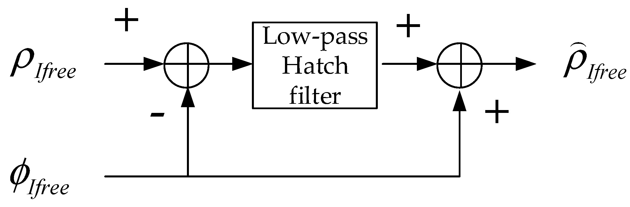
The Ifree filtering algorithm completely detaches the first-order ionospheric effect by taking Ifree combinations of GNSS measurements from two frequencies [9]. Figure 1 presents a typical Ifree filter.

The input of the Ifree filtering algorithm is written as

$${\rho }_{Ifree}={\rho }_{f1}-\frac{1}{\zeta }\left({\rho }_{f1}-{\rho }_{f2}\right)$$

(5)

$${\varphi }_{Ifree}={\varphi }_{f1}-\frac{1}{\zeta }\left({\varphi }_{f1}-{\varphi }_{f2}\right)$$

(6)

where ρ is the range measurement. ϕ is the carrier-phase measurement. $\zeta$ is calculated as $\zeta =1-f_1^2/f_2^2$. A low-pass filter is employed to attenuate the high-frequency noise in the input measurements. The filtered output is given by

$${\stackrel{⌢}{\rho }}_{Ifree}=R+\left({\epsilon }_1-\frac{1}{\zeta }\left({\epsilon }_1-{\epsilon }_2\right)\right)+\frac{1}{\zeta }IFB$$

(7)

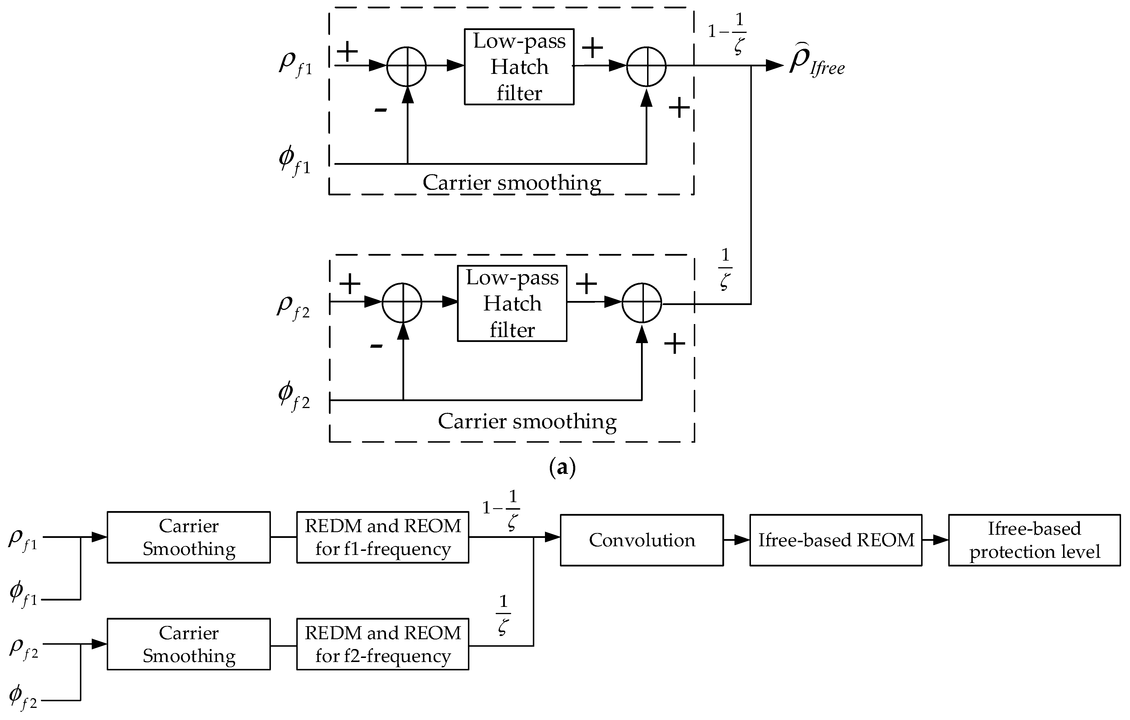
where R represents all common terms in the code and carrier phase measurements, including the true distances between the satellites and users, the satellite and receiver clock biases and the tropospheric delay. $\epsilon$ denotes the filtered errors, including the multipath errors and thermal noise. IFB is the interfrequency bias. Since Ifree-based errors are formed by the combination of two frequencies, they are destined to be larger than single-frequency errors. One can directly estimate the overbounds based on the filtered Ifree-based measurements. However, this method is not adopted in this study. Instead, an equivalent schematic diagram of an Ifree filter and an overbounding framework is given in Figure 2.

The diagram of the Ifree filtering algorithm in Figure 1 can be transformed into the diagram in Figure 2a since Ifree filtering is a linear system. By using the homogeneity property and additivity property, an Ifree-based GBAS can be decomposed into two subsystems, where the measurements are combined after passing through the same low-pass Hatch filter. Based on the equivalent Ifree filtering algorithm, the overall overbounding process is shown in Figure 2b. The REDM and REOM can be established by using the errors of each frequency. Then, the REOM of the Ifree-based GBAS can be obtained by linearly convolving two single-frequency REOMs. The corresponding protection levels can be calculated. An assumption that the Ifree-based overbound is based on the error models of the individual contributions derived from the measurements for two frequencies is adopted. Namely, the overbound is not derived from the direct estimation of the final Ifree-based errors. During sample collection, if the measurements of one frequency are interfered with, the measurements of the other frequency can still be received and modeled. This framework makes full use of the collected samples. Specifically, provided that the measurements can be received continuously, for the Gaussian overbound, the overbounding results of the direct estimation process and the framework in Figure 2b share the same value.

3.2. Single-Frequency REDM Establishment

When the elevation is small, the error presents a heavy tail. Due to the CDF overbound requirement that the location parameter μ must be zero, a two-component GMM REDM is established and given by

$$p(y)={\omega }_1\phi \left(y;0,{\sigma }_1\right)+{\omega }_2\phi \left(y;0,{\sigma }_2\right)$$

(8)

where ${\omega }_1+{\omega }_2=1$. There are three reasons for choosing this 2-component GMM. First, the model minimizes the number of components while providing sufficient flexibility. One component can describe the core, and the other can describe the tails. Both the tight core and the heavy tails can be thoroughly considered [37]. Second, a multicomponent model can be overbounded by a two-component model. Finally, the model can avoid overfitting and nonconvergence in practice. The developed algorithm can be used to estimate the model parameter values.

For high elevations where the heavy tail is absent, the error distribution tends to be a Gaussian distribution [27]. At this point, the EM algorithm fails to converge, so a simple Gaussian overbound may be preferred.

3.3. Single-Frequency REOM Establishment

To construct an REOM, it is indispensable to replace the current parameter values in the REDM with bounds. By increasing or decreasing the parameter values, the REDM with parameters estimated by the EM algorithm can then be overbounded. Provided that ${\sigma }_1$ is much greater than ${\sigma }_2$, the structure of the overbounding model is:

$$p_{OB}(y)=\left({\omega }_1+\Delta \omega \right)\phi \left(y;0,{\sigma }_1+\Delta {\sigma }_1\right)+\left({\omega }_2-\Delta \omega \right)\phi \left(y;0,{\sigma }_2+\Delta {\sigma }_2\right)$$

(9)

where $\Delta \theta =\left(\Delta \omega ,\Delta {\sigma }_1,\Delta {\sigma }_2\right)$ represents the modified value of the parameter $\theta$. As the modified parameters increase, the overbound gradually becomes conservative.

Before calculating the overbounding model via the Louis algorithm, inspired by the existing results [39,40,41], one needs to verify whether the coverage probability equals the nominal confidence level. Theoretically, considering the possible error sources, uncertainty and model error qualification are crucial. The uncertainty comes mainly from a small sample size. The empirical distribution function converges to the underlying CDF with the full probability if the sample size is sufficiently large. However, the empirical distribution of limited samples may not be exactly the same as the underlying distribution in practice. The model error arises mainly because the number of components is restricted. Although the GMM can approximate a real model with an increase in the number of components, it is restrained in practical application environments. Accordingly, Equation (8) is an approximate estimate of the sample data rather than an accurate estimate.

To verify the above statements, data from heavy-tailed distributions are simulated including four-group GMMs from [30,34,37,38] and four typical non-GMMs, i.e., Normal-inverse gamma (NIG) [22], GCET [14], GPO [27] and stable distributions [26]. To better show the disparity between the GMMs and non-GMMs, the samples are classified [36]. If the samples follow a GMM, the group is specified as a correct parametric model. The fitted distribution can approach the underlying distribution. No model error is observed; only an estimation uncertainty is present. The chosen parameters of the correct parametric model are shown in

Table 1. Distributions and parameters of the correct parametric model for testing.

Parameters	Group
	1	2	3	4
${\omega }_1$	0.85	0.95	0.975	0.50
${\sigma }_1$	1.82	0.97	1.50	1.50
${\sigma }_2$	0.75	0.11	0.30	0.50

. The other type of model that disobeys a GMM is called a false parametric model. In this case, both model errors and uncertainties exist. The correct parametric model is considered as a reference. Namely, if the estimation of the correct model is accurate while that of the false model is inaccurate, the existence of model errors is verified. The chosen parameters of the false parametric model are shown in

Table 2. Distributions and parameters of the false parametric model for testing.

Distribution	Parameters
NIG	$\alpha$ = 0.65 $\sigma$ = 0.65 $\beta$ = 0 $\mu$ = 0
GCET	$\sigma$ = 0.8, El = 1.57
GPO	$\gamma$ = 0.03 $\sigma$ = 0.82
Stable	$\alpha$ = 1.95 $\sigma$ = 0.9 $\beta$ = 0 $\mu$ = 0

.

In addition, the true value of the GMM estimation must be determined. For the correct parametric model, the true value, also called the parent parameter, can be determined directly according to the underlying distribution. For a false parametric model, the underlying distribution is no longer a GMM. The optimal value calculated by minimizing the absolute cost function is selected to substitute for the parent parameter [40].

$$\left({\omega }_{opt},{\sigma }_{1,opt},{\sigma }_{2,opt}\right)=\underset{\omega ,{\sigma }_1,{\sigma }_2}{\arg \min }{\displaystyle \underset{-\infty }{\overset{\infty }{\int }}\left|F(z;\omega ,{\sigma }_1,{\sigma }_2)-G\left(z\right)\right|}dz$$

(10)

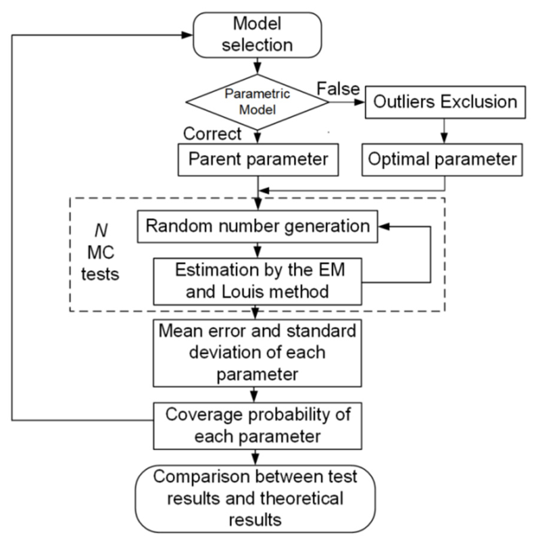
where G(z) represents the underlying distribution of the samples. $F(z;\omega ,{\sigma }_1,{\sigma }_2)$ represents the CDF of the GMM. More importantly, these parameters do not perfectly agree with the underlying distribution. They only present a benchmark for analyzing the existence of model errors. Additionally, obvious outliers need to be ruled out because they can be considered faults and detected by customized monitors in a GBAS. A total of 1000 Monte Carlo (MC) experiments are carried out after selecting the distribution and parameters. The results are then analyzed.

Figure 3 shows the MC simulation procedure. The top loop determines the model type. For each class of models, 2500 independent samples are generated. The mean values and standard deviations of each parameter estimation in the MC simulation are obtained. The nominal confidence level is 95%. Then the coverage probability, namely the probability of the true value falling into the stipulated confidence level, is determined. Finally, the sample type is replaced and the process is repeated until all simulations are accomplished.

Table 3. Correct parametric model results.

Group		1	2	3	4
Absolute value bias	${\omega }_1$	0.001	<0.001	<0.001	<0.001
	${\sigma }_1$	0.005	0.004	0.004	0.002
	${\sigma }_2$	0.002	0.001	<0.001	<0.001
Absolute variance bias	${\omega }_1$	0.002	0.001	<0.001	0.001
	${\sigma }_1$	<0.001	0.001	0.002	0.003
	${\sigma }_2$	<0.001	<0.001	0.001	0.002
Coverage probability	${\omega }_1$	95.6%	94.2%	95.1%	96.2%
	${\sigma }_1$	94.6%	95.5%	95.1%	94.4%
	${\sigma }_2$	94.2%	95.5%	95.7%	95.9%

shows the absolute bias of the MC tests for the correct parametric model. The differences between the values estimated by the EM parameters and the parent value are small. The asymptotic variances of the weighted coefficient and standard deviation estimators closely agree with these calculated by the MC simulation. All coverage probabilities fluctuate slightly around 95%, which shows that the confidence level estimation is accurate when the fitted function can fully approach the underlying function.

Table 4. False parametric model results.

Group		1	2	3	4
Absolute value bias	${\omega }_1$	0.047	0.028	0.011	0.002
	${\sigma }_1$	0.136	0.281	0.176	0.151
	${\sigma }_2$	0.032	0.013	0.028	0.004
Absolute variance bias	${\omega }_1$	0.010	0.001	<0.001	<0.001
	${\sigma }_1$	0.023	0.020	0.148	0.134
	${\sigma }_2$	0.006	<0.001	0.006	<0.001
Coverage probability	${\omega }_1$	55.6%	97.8%	82.7%	81.6%
	${\sigma }_1$	53.6%	61.7%	59.6%	68.6%
	${\sigma }_2$	57.5%	86.2%	86.3%	84.4%

shows the statistics of the MC tests with the false parametric model. It is apparent that bias values increase obviously and that the coverage probability of each parameter value is lower than the nominal value of 95%. Compared with the correct parametric model results, the statistical value of the experimental data disagrees with the calculated value derived from the analytical formula. This disagreement emphasizes the influence of the model errors on the estimation accuracy. The results indicate that the model errors and the estimation uncertainty should both be considered if the samples cannot be guaranteed to come from a GMM.

To ensure that the estimation results are accurate, the coverage probability must be improved. Thus, an additional bias is required to fuse the uncertainties and model errors. Considering that the parameters fluctuate greatly with the properties of the underlying distribution, a nonparametric bootstrapping method is used [15]. Bootstrapping generates many randomly drop-back resampled datasets from the original set. For each resampled data set, a GMM is fitted to perform the parameter estimation process. The additional bias is adjusted and checked for each bootstrap sample to determine whether the coverage probability approaches the nominal value.

Table 5. Additive bias values to be compensated.

Parameters	Distribution
	NIG	GCET	GPO	Stable
$\Delta {\omega }_1$	0.094	0	0.021	0.011
$\Delta {\sigma }_1$	0.276	0.088	0.271	0.281
$\Delta {\sigma }_2$	0.059	0.005	0.030	0.007

shows the sample values that need to be compensated.

When both errors and uncertainties are considered, the PDF of the final single-frequency overbounding distribution is given by

$$p_{OB}(y)=\left(\omega +\Delta {\omega }_{error}\right)\varphi \left(y;0,{\sigma }_1+\Delta {\sigma }_{1,error}\right)+\left(1-\omega -\Delta {\omega }_{error}\right)\varphi \left(y;0,{\sigma }_2+\Delta {\sigma }_{2,error}\right)$$

(11)

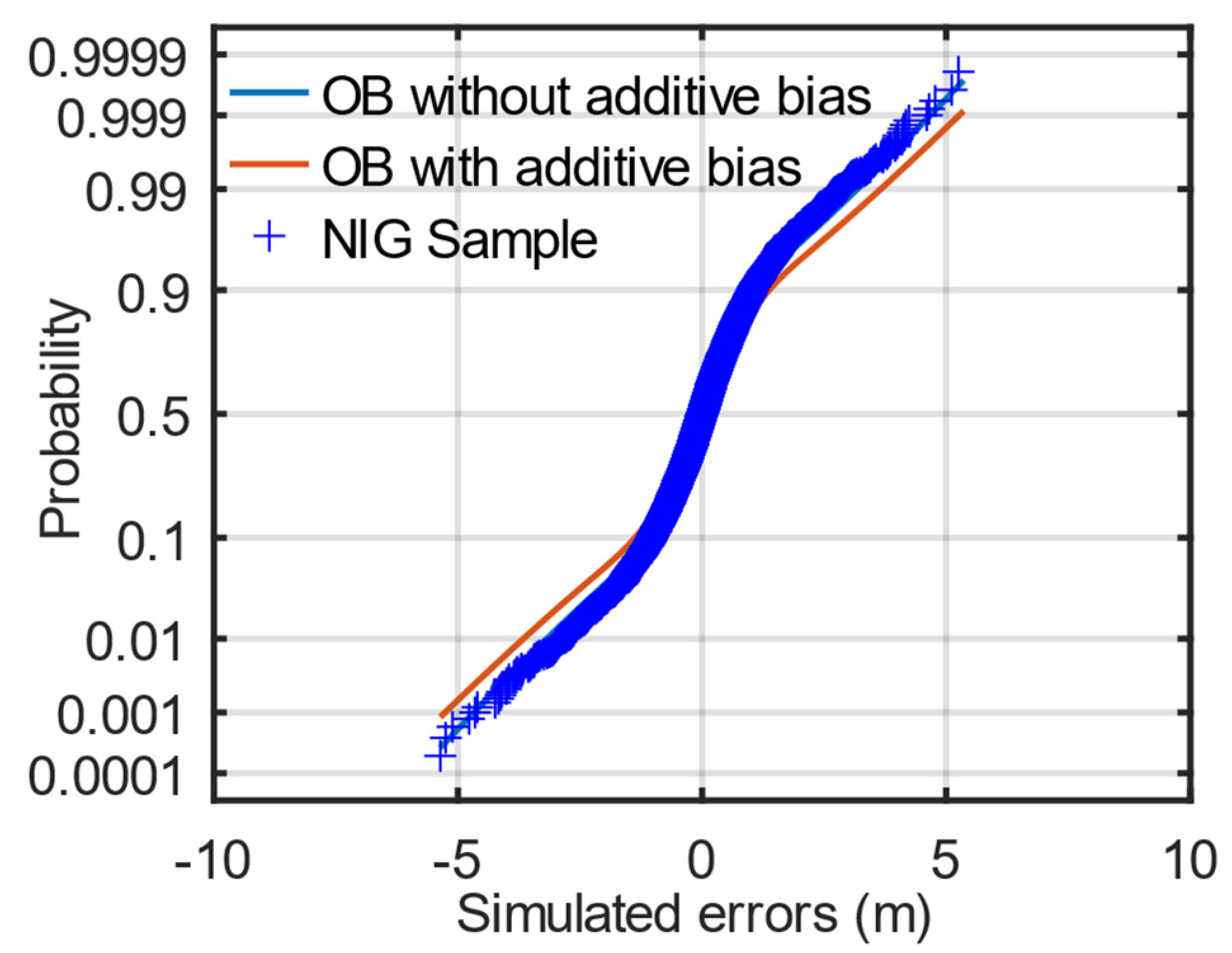
where $\Delta {\theta }_{error}=\left(\Delta {\omega }_{error},\Delta {\sigma }_{1error},\Delta {\sigma }_{2error}\right)$ represents the summary of the impacts of model errors and statistical uncertainty. Figure 4 shows the CDFs of the overbounds with and without additive bias, providing that the distribution of the samples obeys the NIG distribution. The y-axis is scaled by the standard Gaussian distribution to explicitly show tails. After adding the additive bias, the function better overbounds the distribution of simulated samples.

In conclusion, compared with the existing single-frequency GMM overbounds in Section 3.2, the proposed GMM fully considers the uncertainties of all parameters, including the weighted coefficient and both variances. A non-Gaussian overbound is redesigned by using a novel form that is preserved under convolution. This is the original contribution of this study, and it can be extrapolated to solve analogous overbounding problems in single-frequency SBASs, ARAIM systems and integrated navigation systems [25,42].

3.4. Ifree-Based REOM Establishment

The REOM for an Ifree-based GBAS is established in this section. It is crucial to note that convolution is required to obtain Ifree-based overbounds. If a single-frequency overbound does not possess closure under convolution, the results of the corresponding numerical calculation do not obey any explicit distribution. Consequently, the overbounding information cannot be broadcast by limited parameters through the signal channel. The mathematical properties of the overbounding distribution are required.

To overbound Ifree-based errors, the overbounding model for the distribution of each frequency is shown as follows:

$$p_{OB,}{}_i\left(y\right)={\omega }_i{}_{,1}\phi \left(y;0,{\sigma }_i{}_{,1}\right)+{\omega }_i{}_{,2}\phi \left(y;0,{\sigma }_i{}_{,2}\right)$$

(12)

where i = 1 and 2 represent different frequencies. Other parameters have the same meanings as those in (9). Assuming that the errors of the Ifree code measurements are independent, the overbounding property is still maintained after the convolution process [43]. Because a GMM is preserved under convolution, the PDF of the Ifree-based overbound is as follows:

$$\begin{array}{l}{p}_{OB}{}_{,Ifree}\left(y\right)\\ ={\omega }_{1,1}{\omega }_{2,1}\phi \left(y;0,\sqrt{{\left(1-\frac{1}{\zeta }\right)}^2{\sigma }_{1,1}^2+{\left(1-\frac{1}{\zeta }\right)}^2{\sigma }_{2,1}^2}\right)+{\omega }_{1,1}{\omega }_{2,2}\phi \left(y;0,\sqrt{{\left(1-\frac{1}{\zeta }\right)}^2{\sigma }_{1,1}^2+{\left(\frac{1}{\zeta }\right)}^2{\sigma }_{2,2}^2}\right)\\ +{\omega }_{1,2}{\omega }_{2,1}\phi \left(y;0,\sqrt{{\left(\frac{1}{\zeta }\right)}^2{\sigma }_{1,2}^2+{\left(1-\frac{1}{\zeta }\right)}^2{\sigma }_{2,1}^2}\right)+{\omega }_{1,2}{\omega }_{2,2}\phi \left(y;0,\sqrt{{\left(\frac{1}{\zeta }\right)}^2{\sigma }_{2,1}^2+{\left(\frac{1}{\zeta }\right)}^2{\sigma }_{2,2}^2}\right)\\ ={\omega }_1\phi \left(y;0,{\sigma }_1\right)+{\omega }_2\phi \left(y;0,{\sigma }_2\right)+{\omega }_3\phi \left(y;0,{\sigma }_3\right)+{\omega }_4\phi \left(y;0,{\sigma }_4\right)\end{array}$$

(13)

According to Equation (13), the PDF of the Ifree errors is a 4-component GMM. If the overbound is directly established from Ifree-filtered errors, the overbound is a two-component GMM that provides less accuracy and flexibility. Notably, a four-component GMM yields a better illustration of the trend of the filtered errors. In conclusion, Ifree-based overbounds are established and their protection levels can be obtained as described in the overbounding framework. In other scenarios where similar linearity exists, Equation (13) can be applied to address corresponding overbounding approaches.

3.5. Ifree-Based Protection Level Calculation Utilizing GMM Overbounds

GBAS protection levels are used in the position domain to ensure the integrity, while the parameters of the error distribution characteristics are broadcast in the range domain. Therefore, it is indispensable to project the overbound to the protection levels to ensure integrity. Since the vertical errors are greater than the lateral errors, the vertical protection level (VPL) is taken as an example.

The position error E_v is a linear combination of the range errors of all utilized satellites, which is given in [34].

$$E_v={\displaystyle \sum _{k=1}^N{S}_{3,k}{E}_k}$$

(14)

where S_3,k is the kth of the vertical-position row element of the projection matrix S, whose derivation is provided in [12]. N represents the number of visible satellites. E_k is the kth error of the corresponding satellites covering all range error sources, including noise, multipath errors, tropospheric errors and so on. Consequently, the PDF of the position errors is determined by those of the GBAS range errors.

Only the uncertainties from the ground multipath errors and the thermal noise of Ifree-based errors are considered in (13). Namely, the original GMM overbound only covers the uncertainties from multipath errors and thermal noise. Additional uncertainties derived from airborne errors, tropospheric errors and IFB need to be taken into account. Gaussian models developed by [44,45] are utilized rather than a remodeling of these errors. Then, a final GMM overbound can be obtained by convolving the Gaussian distributions with (13) to cover all the potential errors. Due to convolution invariance, the final overbound can be calculated rapidly and directly. In the final GMM overbound, the weight coefficient remains the same and the variance is the sum of the original variance and the variance of the dditional errors.

Then, the PDF of the position-error overbound is provided by N successive convolution integrals as follows:

$$p_{OB,v}\left(z\right)=\frac{1}{{\displaystyle \prod _{n=1}^N{S}_{3,n}}}{\displaystyle {\int }_{-\infty }^{\infty }\cdots }{\displaystyle {\int }_{-\infty }^{\infty }{p}_{OB,1}\left(\frac{z-{\epsilon }_2}{S_{3,1}}\right)}{p}_{OB}{}_{,2}\left(\frac{{\epsilon }_2-{\epsilon }_3}{S_{3,2}}\right)\dots p_{OB,N}\left(\frac{{\epsilon }_N}{S_{3,N}}\right)d{\epsilon }_2\dots d{\epsilon }_N$$

(15)

where p_OB,i is the PDF of the ith overbound from the ith visible satellite. For overbounds that cannot be preserved under convolution, Equation (15) must be computed numerically, which is overwhelmingly complicated for an airborne facility. Fortunately, the GMM satisfies convolution invariance. Thus, calculating Equation (15) using the GMM overbound requires a computational load similar to that of the Gaussian method. The closed-form PDF of the Ifree-based bound in the position domain is shown as follows

$$p_{GMMOB,v}(z)={\displaystyle \sum _{i=1}^N{\displaystyle \sum _{k_i=1}^4\dots {\displaystyle \sum _{k_1=1}^4{\omega }_{i,k_i}}\dots {\omega }_{1,k_i}\phi \left(z,0,\sqrt{S_{3,i}^2{\sigma }_{n,k_n}^2+\dots +S_{3,1}^2{\sigma }_{1,k_{{}_1}}^2}\right)}}$$

(16)

where k_i represents the kth component corresponding to the ith visible satellite. ${\omega }_{\mathrm{i},k_i}$ represents the weight coefficient. ${\sigma }_{n,k_n}^2$ represents the corresponding variance. Ignoring the vertical difference caused by the filtering time [44], the final VPL can be calculated as

$$VPL=F_{{}^{GMMOB,v}}^{-1}\left(P_{IR}\right)$$

(17)

where P_IR is the allocated integrity risk, F_GMMOB,v is the integral of (16), and F⁻¹ is the inverse function of F. Although additional computations may be required to solve Equation (17), the cost is much less than that of numerical convolution.

Due to its low level of freedom and conservative core, the Ifree filtering algorithm increases Gaussian overbounds by 2.6 or more when receiving L1 and L5 GPS signals. The same situations apply to Ifree-based GBAS when receiving B1C and B2a BDS signals. The VPLs are too conservative, implying a high probability of exceeding prescribed alarm alerts. Then, a false alert is triggered, and availability is lost. Conversely, for GMM overbounds, although some items with large variances exist in F_GMMOB,v, the corresponding coefficients are quite small and far lower than the integrity risk, thus having little impact on the final VPLs. Therefore, it can be foreseen that the Ifree-based VPLs based on a GMM are not as conservative as those based on the Gaussian method.

However, the number of components in Equation (16) increases exponentially. If this condition is left untreated, obtaining the quantiles of the multicomponent GMM may even require more computations than numerical convolution. This significantly increases the computational load required to solve Equation (17). One available way to obtain a high speed is to control the number of components without introducing additional integrity risk. A GMM with more components can be overbounded by fewer components. A simple proof is as follows. A larger variance indicates a heavier tail [36]. Provided that the variance of a given component is not the largest, one can increase this variance to the largest value and merge the items with the same variance while retaining the core parts. The net effect is a reduction in the number of components. Thus, components with similar variances can be merged upward to reduce the number of components and the computational complexity. Note that if the number of merged components is too small, the conservatism is increased significantly. For the sake of balance, empirical advice suggests reducing the number of components to 10. This may make the results slightly conservative, while the cost is feasible.

4. Results

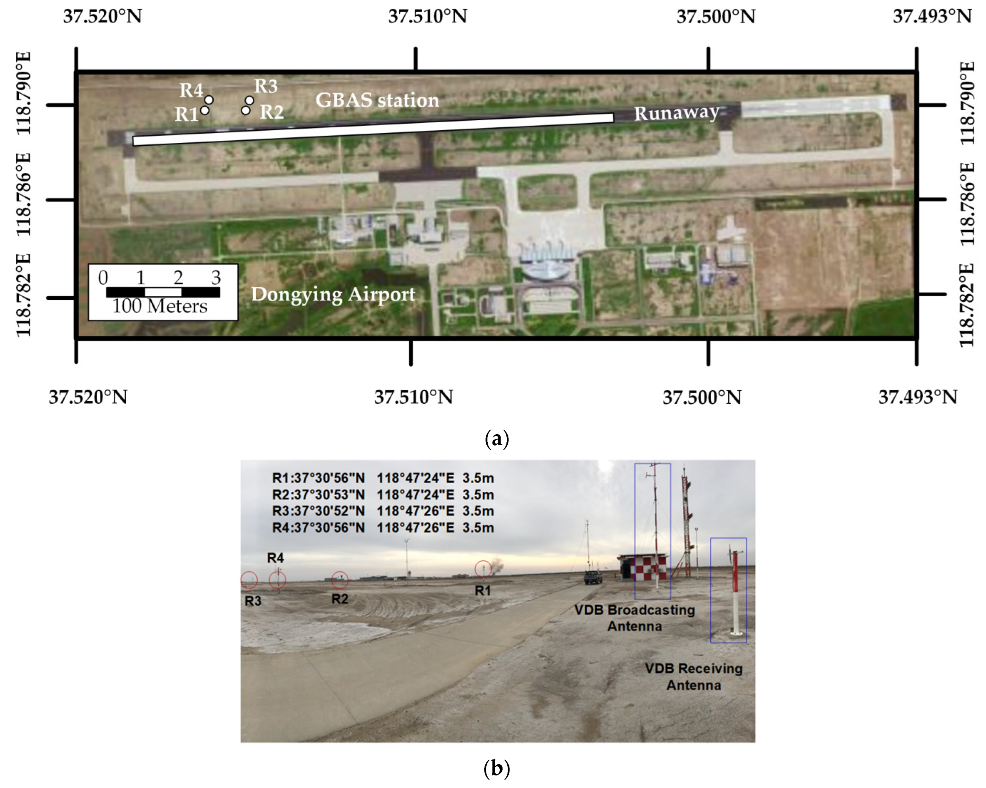
Real-world BDS data from a GBAS are implemented to test the performance of the developed overbounds. This experiment is conducted at the Dongying Airport, where the GBAS prototypes are developed by Beihang University and Tianjin 712 Communication & Broadcasting Co., Ltd. in Tianjin, China [46]. A top view of the whole airport is shown in Figure 5a, and the configuration of the experimental setup is shown in Figure 5b. The red circles are the four reference stations and the blue rectangles are the very high frequency data broadcast (VDB) antennas. All four reference stations are equipped with the same antenna, and their positions are precisely calibrated. The BDS signals received by the reference stations are B1I and B3I signals, with carrier frequencies of 1561.098 and 1268.520 MHz, respectively [47]. These two types of signals are used to simulate the Ifree-based GBAS. Although these signals are not specified for a future BDS GAST-F, the results can highlight the expected performance level when the B1C and B2a signals become available [48]. In this case, ζ is calculated as 0.339. The filtering time is set as 100 s.

The GMM overbound is compared with two Gaussian overbounds, including the conservative REDM based on the GCET model and the accurate REDM based on the EVT model [14,25]. Regardless of the utilized REDM, VPLs based on the Gaussian overbound of the Ifree-based GBAS are approximately 2.5 times larger than those of the single-frequency GBAS. If the Gaussian inflation factor is still large, the VPLs can be extremely conservative. The confidence level of the overbound is set as 0.95.

The offline data were collected from 10 November 2019, to 19 January 2020, in the real environment described above. The data processing steps included data collection and grouping, which were performed by following the procedures presented in [20]. The range errors collected from the prototype were binned at intervals of 5°. Due to the limited amount of data, the errors of different frequencies were mixed as suggested by [49]. This strategy works under the implicit assumption that the errors of both frequencies share the same distribution.

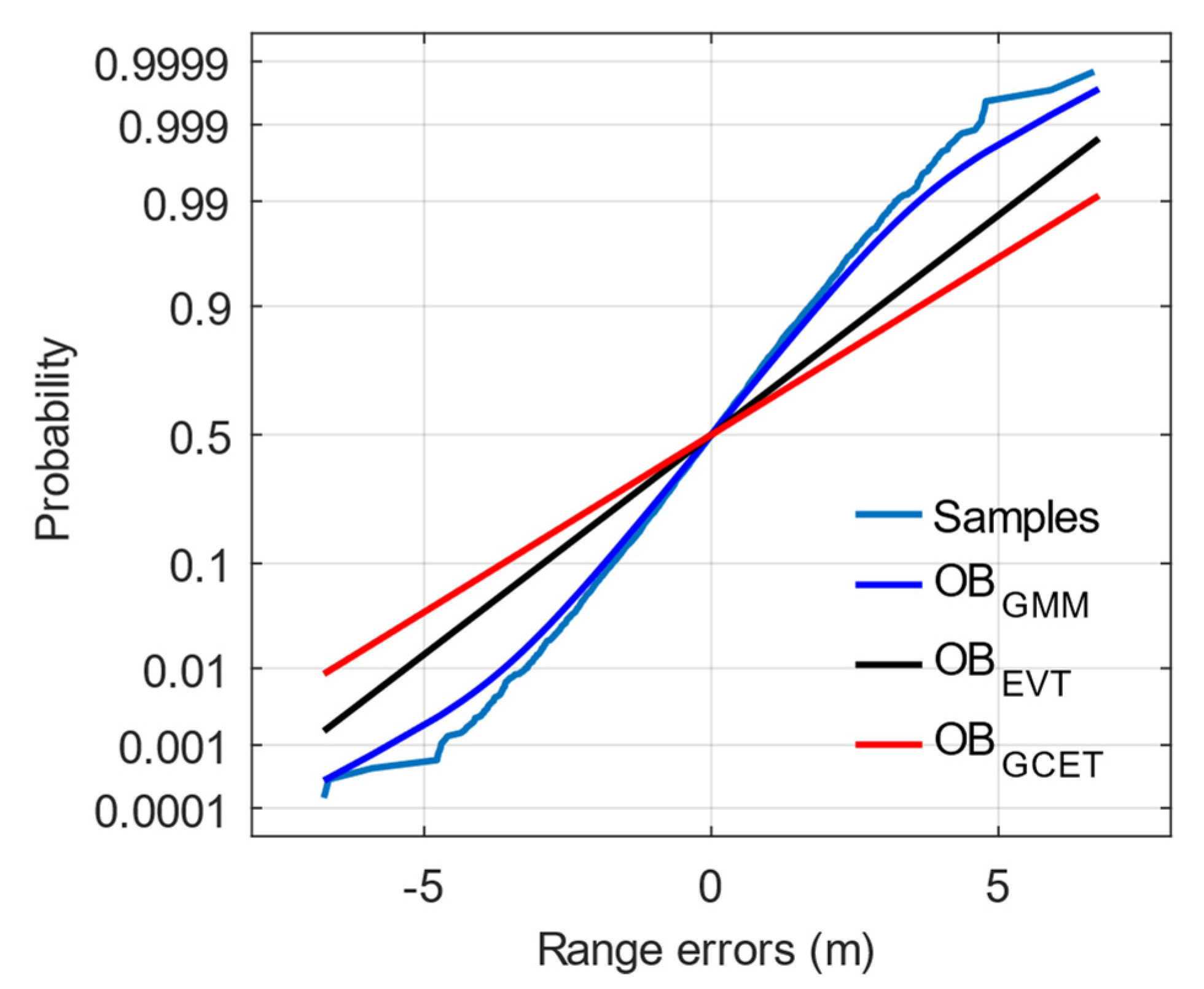
For a quantitative range domain overbounding performance comparison, the sum of difference (SUMD) is introduced [11]. It can describe the differences between the underlying distribution and the overbounds. Our study normalizes the SUMD to eliminate the effects of sample size. The average SUMD, i.e., $\stackrel{\_\_\_\_\_\_\_\_\_}{SUMD}$, is given as

$$\stackrel{\_\_\_\_\_\_\_\_\_}{SUMD}=\frac{1}{N_{bin}}{\displaystyle \sum _{i=1}^{N_{bin}}\left|F_{OB}\left(x_i\right)-F\left(x_i\right)\right|}$$

(18)

where $N_{bin}$ represents the total number of sample points in an elevation bin. A smaller $\stackrel{\_\_\_\_\_\_\_\_\_}{SUMD}$ indicates a tighter overbound. Without loss of generality, an elevation bin from 15° to 20° demonstrates the capability of the GMM to characterize the heavy tails in

Table 6. Distribution parameters of different overbounds at elevation bins from 15° to 20°.

Distribution	Parameters	$\stackrel{\_\_\_\_\_\_\_\_\_}{SUMD}$
GMM	${\omega }_1$$=0.0027 {\sigma }_1$ = 2.98	0.0141
	${\omega }_2$$=0.0493 {\sigma }_2$ = 2.60
	${\omega }_3$$=0.0493 {\sigma }_3$ = 2.00
	${\omega }_4$$=0.8987 {\sigma }_4$ = 1.37
EVT-Gaussian [14]	$\sigma$ = 2.2855	0.0835
GCET-Gaussian [25]	$\sigma$ = 2.8308	0.1110

and Figure 6. The parameters of the GMM overbound correspond to Equation (13), and Gaussian overbound are characterized by the parameter $\sigma$. The y-axis in Figure 6 is scaled by the standard Gaussian distribution to highlight the tails. The results show that the GMM method provides a closer overbound to the sample distribution than that of the Gaussian method in both the core and tail parts. Therefore, the improved GMM overbound can better represent the trend of the original distribution than the Gaussian methods.

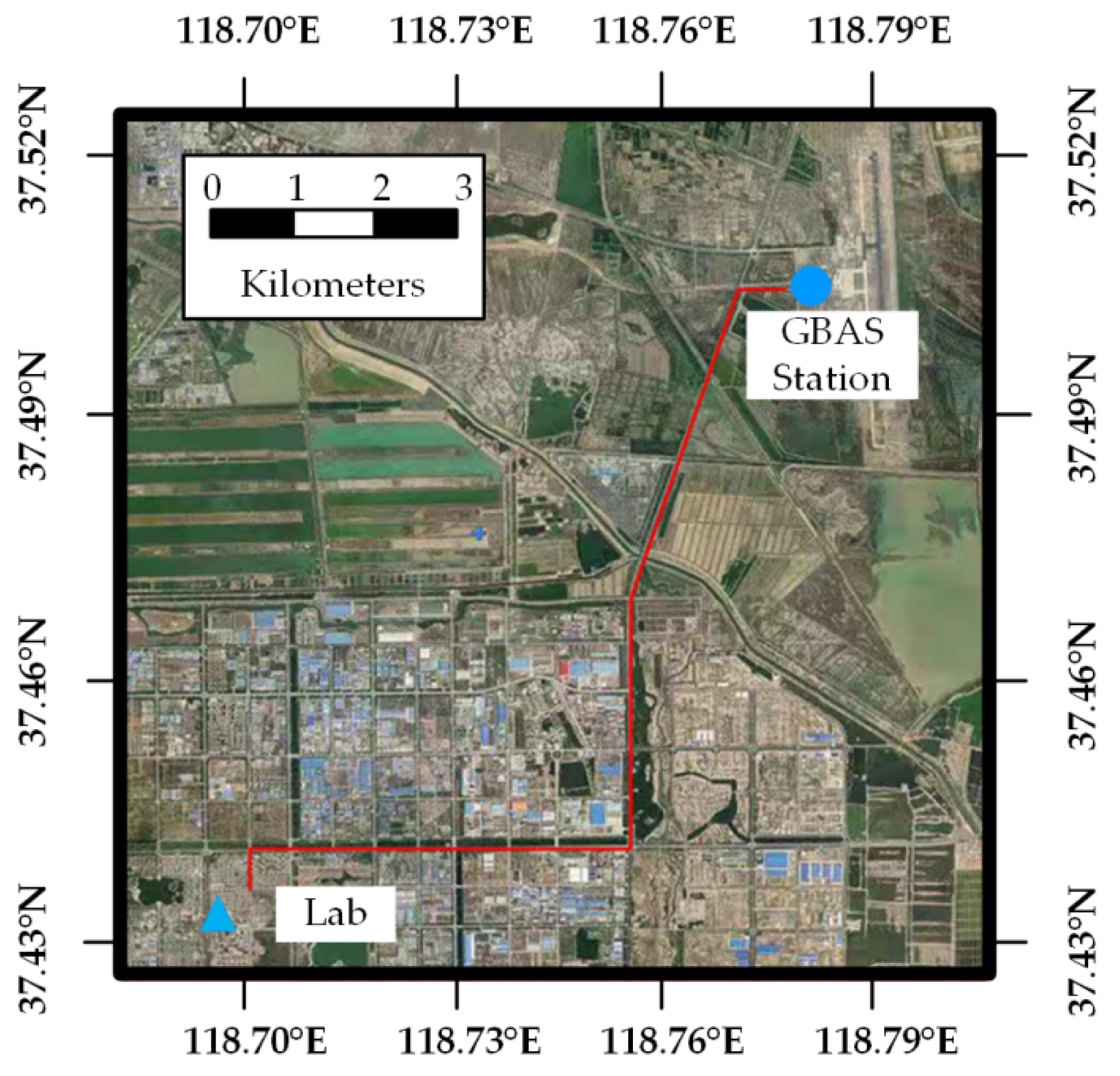
To assess the performance of the VPLs based on the proposed overbound in the real environment, a road test was carried out near the GBAS station on 25 January 2021. A receiver deployed in a land vehicle that collects the BDS data at a frequency of 0.5 Hz is assumed to be the dynamic user. The location of the GBAS station and the reference trajectory of the vehicle are illustrated in Figure 7. The experiment was repeated three times along this trajectory. To prevent the influence of nonline-of-sight signals, only seven satellites whose visibilities remained unchanged during the overall process were selected. These satellites included four GEO satellites (C01, C02, C03 and C04) and three IGSO satellites (C06, C09 and C10) [47]. In addition, the test vehicle was furnished with a receiver as the user receiver, along with another receiver in the lab as the base station to conduct real-time kinematic (RTK) positioning. The RTK solutions minus the Ifree position results are assumed to be the actual errors for the entire road test.

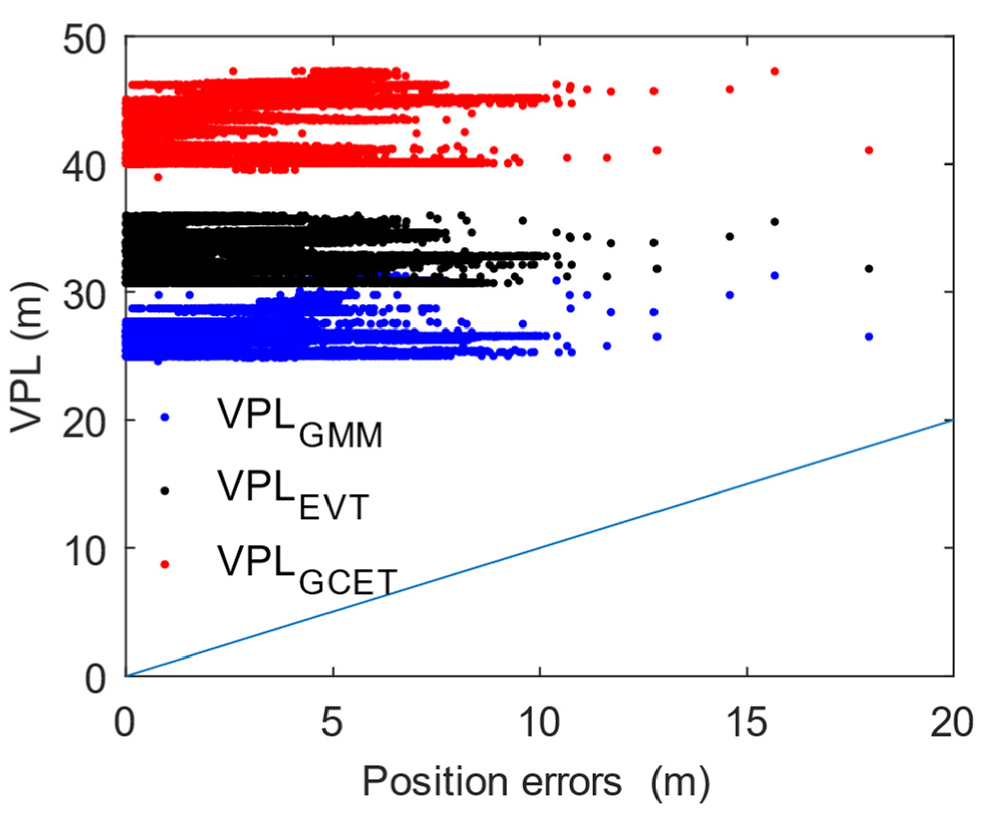
The VPLs are calculated by using the road test data. An integrity risk at 10⁻⁹ is taken as an example. Figure 8 shows the errors against the VPLs calculated by different methods. Figure 8 is divided by a diagonal line, at which position errors equal the VPLs. No error exceeds the VPLs since all points are above the diagonal line in this test. The integrity appears to be preserved. In addition, the position errors in the urban environment are larger than those in the aviation environment [50]. The GMM overbound does not introduce an integrity risk under adverse conditions. The statistical results of the VPLs are summarized in

Table 7. Statistics of observed VPLs (in meters).

Distribution	Mean	Maximum	Standard Derivation
GMM	26.74	31.29	1.49
EVT-Gaussian	32.83	36.01	1.62
GCET-Gaussian	43.03	47.39	2.25

. One important result is that the GMM VPLs are smaller than the Gaussian VPLs. Compared with the Gaussian VPL whose REDM is EVT, the GMM VPLs reduce the mean value by approximately 19%, maximum value by approximately 13% and dispersion by approximately 8%. Lower VPLs lead to more availability. Gaussian VPLs are more likely to fail to perform a navigation operation due to conservatism.

5. Discussion

5.1. VPLs versus Alarm Limits

We have shown that our proposed overbounds can achieve excellent performance in characterizing the error distributions in the range domain and tightening the VPLs in position domain. Although the GMM VPLs are smaller than the Gaussian VPLs, it is apparent that they far exceed the 10-m alarm limits [16]. This is mainly because the position errors are relatively large. The following three measurements can make an Ifree-based GBAS feasible. First, as more errors become available, the distribution of GBAS errors can be precisely characterized [27]. The accuracy of the error distribution estimation for each frequency can be increased. Second, it is preferable to employ the B1C and B2a signals for the BDS GAST-F [47]. The frequency difference between the two signals is smaller than that between the B1I and B3I signals. This means that those introduced by the B1C and B2a signals are smaller than those of the B1I and B3I signals. Finally, considering the outstanding performance of the current BDS-3 constellation and future multiconstellation satellites [51], the overall satellite geometry can be improved. The position errors can be reduced. If these conditions can be met, the position accuracy will be enhanced. Therefore, the availability of the Ifree-based GBASs can be enhanced in association with a tighter GMM overbound.

5.2. Computational Load

Theoretically, any convolution-invariant distribution does not result in much additional computational load. Thus, this type of overbound performs much more rapidly than an overbound that requires numerical convolution. However, the calculation of the quantiles of non-Gaussian distribution are inevitably more resource-consuming than simple Gaussian distributions. Obtaining quantiles of the integrity risk in the position domain as Equation (17) may introduce the computational load. Thus, the times required to calculate the VPLs with different overbounding methods including the traditional Gaussian, the GMM, the stable [26] and the GPO distributions [27], are compared. As a reference, the calculation time is normalized by the time of the Gaussian distribution. The calculation software is OCTAVE, and the accuracy is 0.005 m, as suggested by [12].

Table 8. Average computational time to calculate the VPLs with different overbounding methods. The times are the relative times compared with that of the Gaussian overbound. A lower time indicates less computational load.

Distribution	GMM	Stable	GPO
Relative time	64	423	≈60,000

summarizes the relative times taken by different overbounds compared with that of the Gaussian overbound. It can be seen that GMM overbounds are approximately 60 times slower than the Gaussian summations. It is also interesting to see that the calculation time required for the GMM VPLs is much smaller than the stable overbound which also has convolution invariance. This means that the complexity of solving the quantile of the GMM lies between those of the simple Gaussian distribution and the complex stable distribution. All methods are much faster than the GPO method that leverages numerical calculation. Considering the contribution of the proposed method to the accurate overbound, it is worth the slightly extra computational load to attain tighter VPLs. In conclusion, the GMM is an appealing method for overbounding GBAS range errors.

5.3. Limitation

The proposed method possesses some possible limitations. First, the additive bias determination in Equation (11) is highly empirical and depends on the properties of the underlying distribution. For each set of samples, the additive bias estimation requires a high computational cost. Hence, bootstrapping is not suitable if the user chooses to determine the REOM in real time. The second limitation concerns the limited VDB capacity in broadcasting the integrity information with the multiparameter in navigation messages when using a BDS-3 GBAS [52]. The current messaging method allows users to compute the variance of each range error every time, which means that only one parameter needs to be broadcast. However, for the GMM overbound, the user needs the information broadcast by the GBAS ground-subsystem station with three parameters. A minor modification to the current message content is needed, which requires high VDB capacity. This limitation is even more pronounced if the user chooses to make these parameters vary with the satellite [37]. The last issue concerns the frequency correlation. Our work is based on the assumption that the errors of different frequencies are independent, whereas range errors appear to show positive statistical correlations [43]. Namely, the positive correlation of errors between different frequencies reduces the uncertainty of the final error after Ifree filtering, which makes the protection levels loose. This correlation is an inevitable challenge for the future application of Ifree-based GBASs.

6. Conclusions and Perspectives

Ifree filtering can effectively mitigate the ionospheric anomalies of a GBAS, but it amplifies the noise and thus affects availability. An overbounding framework for Ifree-based GBAS ranging errors based on a GMM is proposed to boost availability. A two-component GMM model is established to fit single-frequency, heavy-tailed errors. It is found that the general uncertainty estimation method is inaccurate by using an MC test. A non-parametric bootstrap is utilized to compensate for this inaccuracy. Then, an accurate GMM overbound for the Ifree-based GBASs is established. Closed-form VPLs are derived without introducing much computational cost. A road test shows that the proposed GMM overbound tightens the VPLs without introducing much computational load relative to other non-Gaussian overbounds. Overall, the GMM overbound approach is an encouraging alternative for calculating tighter position error bounds. The contributions of our work can be summarized as follows.

• Our work proposes an overbounding framework for a dual-frequency GBAS.
• Our work redesigns a novel form of the GMM overbound to rigorously characterize heavy-tailed distributions. To determine whether the GMM parameter estimation approach is accurate, our work evaluates its point estimation accuracy and confidence interval estimation accuracy.
• To calculate the protection levels, our work derives Ifree-based protection levels by using the GMM overbound, which optimizes the availability without significantly increasing the computational load.

Future work will be carried out to make GMM overbounds more useful for the GBAS community. First, multipath errors have advanced degrees of statistical correlation between frequencies. How to characterize these correlations constitutes part of our future work. Second, the performance of a real flight test in varying aviation environments needs to be evaluated. Finally, the proposed overbound is only suitable for cases that have linear relationships. Future work will involve studying the cases in which potential nonlinearity exists.

References

1. Hein, G.W. Status, perspectives and trends of satellite navigation. Satell. Navig. 2020, 1, 22. [Google Scholar] [CrossRef] [PubMed]
2. Barnes, D. GPS Status and Modernization; Munich Satellite Navigation Summit: Munich, Germany, 2019. [Google Scholar]
3. Zrinjski, M.; Barković, D.; Matika, K. Development and Modernization of GNSS. Geodetski List 2019, 73, 45–65. [Google Scholar]
4. Pereira, L.M.; Pullen, S.; de Oliveira Moraes, A.; Santos, J.S. Ground-Based Augmentation Systems Operation in Low Latitudes—Part 1: Challenges, Mitigations, and Future Prospects. J. Aerosp. Technol. Manag. 2021, 13, e4621. [Google Scholar] [CrossRef]
5. Wang, S.; Zhai, Y.; Zhan, X. Characterizing BDS signal-in-space performance from integrity perspective. Navigation 2021, 68, 157–183. [Google Scholar] [CrossRef]
6. Gao, Z.; Fang, K.; Zhu, Y.; Wang, Z.; Guo, K. An Ionospheric Anomaly Monitor Based on the One Class Support Vector Algorithm for the Ground-Based Augmentation System. Remote Sens. 2021, 13, 4327. [Google Scholar] [CrossRef]
7. Wang, Z.; Li, T.; Li, Q.; Fang, K. Impact of Anomalous Ionospheric Gradients on GBAS in the Low-Latitude Region of China. GPS Solut. 2021, 25, 2. [Google Scholar] [CrossRef]
8. Yuan, Y.; Ou, J. Auto-covariance estimation of variable samples (ACEVS) and its application for monitoring random ionospheric disturbances using GPS. J. Geod. 2001, 75, 438–447. [Google Scholar] [CrossRef]
9. Suzuki, K.; Pullen, S.; Enge, P.; Ono, T. Evaluation of Dual-Frequency GBAS Performance using Data from Public Receiver Networks. In Proceedings of the ION GNSS 2010, Institute of Navigation, Portland, OR, USA, 21–24 September 2010; pp. 2592–2602. [Google Scholar]
10. Wang, Z.; Yin, Y.; Song, D.; Fang, K.; Li, Q.; Li, X. Dual Smoothing Ionospheric Gradient Monitoring Algorithm for Dual-Frequency BDS GBAS. Chin. J. Aeronaut. 2020, 33, 3395–3404. [Google Scholar] [CrossRef]
11. Hwang, P.Y.; Mcgraw, G.A.; Bader, J.R. Enhanced Differential GPS Carrier-Smoothed Code Processing Using Dual-Frequency Measurements. Navigation 1999, 46, 127–137. [Google Scholar] [CrossRef]
12. Larson, J.D.; Gebre-Egziabher, D.; Rife, J. Improving Navigation System Availability Using Gaussian-Pareto Overbounding. In Proceedings of the ION GNSS+ 2019, Institute of Navigation, Miami, FL, USA, 16–20 September 2019; pp. 3153–3161. [Google Scholar]
13. Dautermann, T.; Mayer, C.; Antreich, F.; Konovaltsev, A.; Belabbas, B.; Kalberer, U. Non-Gaussian Error Modeling for GBAS Integrity Assessment. IEEE Trans. Aerosp. Electron. Syst. 2012, 48, 693–706. [Google Scholar] [CrossRef]
14. Shively, C.; Braff, R. An Overbound Concept for Pseudorange Error from the LAAS Ground Facility. In Proceedings of the ION AM 2000, Institute of Navigation, San Diego, CA, USA, 26–28 June 2000; pp. 661–671. [Google Scholar]
15. Xue, R.; Wang, Z. A Novel LAAS Pseudo-Range Error over-Bound Method Based on Improved Pseudo-Range Error Distribution Model. Chin. J. Aeronaut. 2013, 26, 638–645. [Google Scholar] [CrossRef] [Green Version]
16. Sung, Y.; Lin, Y.; Yeh, S.; Jan, S. A Dual-frequency Ground Based Augmentation System Prototype for GPS and BDS. In Proceedings of the ION GNSS+ 2019, Institute of Navigation, Miami, FL, USA, 16–20 September 2019; pp. 628–636. [Google Scholar]
17. Kelly, R.J.; Davis, J.M. Required Navigation Performance (RNP) for Precision Approach and Landing with GNSS Application. Navigation 1994, 41, 1–30. [Google Scholar] [CrossRef]
18. DeCleene, B. Defining Pseudorange Integrity—Overbounding. In Proceedings of the ION GPS 2000, Institute of Navigation, Salt Lake City, UT, USA, 19–22 September 2000; pp. 1916–1924. [Google Scholar]
19. Rife, J.; Pullen, S.; Enge, P.; Pervan, B. Paired Overbounding for Nonideal LAAS and WAAS Error Distributions. IEEE Trans. Aerosp. Electron. Syst. 2006, 42, 1386–1395. [Google Scholar] [CrossRef]
20. Zhang, Y.; Xiao, Z.; Li, P.; Tang, X.; Ou, G. Conservative Sensor Error Modeling Using a Modified Paired Overbound Method and Its Application in Satellite-Based Augmentation Systems. Sensors 2019, 19, 2826. [Google Scholar] [CrossRef] [PubMed] [Green Version]
21. Lee, J.; Pullen, S.; Enge, P. Sigma Overbounding Using a Position Domain Method for the Local Area Augmentaion of GPS. IEEE Trans. Aerosp. Electron. Syst. 2009, 45, 1262–1274. [Google Scholar] [CrossRef]
22. Braff, R.; Shively, C. A Method of Over Bounding Ground Based Augmentation System (GBAS) Heavy Tail Error Distributions. J. Navig. 2005, 58, 83–103. [Google Scholar] [CrossRef]
23. Zhao, L.; Zhang, J.; Li, L.; Yang, F.; Liu, X. Position-Domain Non-Gaussian Error Overbounding for ARAIM. Remote Sens. 2020, 12, 1992. [Google Scholar] [CrossRef]
24. Blanch, J.; Walter, T.; Enge, P. Gaussian Bounds of Sample Distributions for Integrity Analysis. IEEE Trans. Aerosp. Electron. Syst. 2019, 55, 1806–1815. [Google Scholar] [CrossRef]
25. Fang, K.; Zhu, Y.; Xue, R.; Fang, J. Extreme Value Overbounding with the Aid of Samples from Distribution Core in GNSS Augmentation System. In Proceedings of the ION PNT 2015, Institute of Navigation, Honolulu, HI, USA, 20–23 April 2015; pp. 905–911. [Google Scholar]
26. Xue, R.; Wang, Z.; Zhu, Y. Upper bound estimation of positioning error for ground-based augmentation system. GPS Solut. 2017, 21, 1781–1790. [Google Scholar] [CrossRef]
27. Larson, J.D.; Gebre-Egziabher, D.; Rife, J.H. Gaussian-Pareto Overbounding of DGNSS Pseudoranges from CORS. Navigation 2019, 66, 139–150. [Google Scholar] [CrossRef] [Green Version]
28. Tan, K.; Chu, M. Estimation of portfolio return and Value at Risk using a class of Gaussian mixture distributions. Int. J. Bus. Financ. Res. 2012, 6, 97–107. [Google Scholar]
29. Wilson, R. Multiresolution Gaussian Mixture Models: Theory and Applications; Department of Computer Science, University of Warwick: Coventry, UK, 1999. [Google Scholar]
30. Shively, C. Comparison of LAAS error bounding concepts. In Proceedings of the ION NTM 2001, Institute of Navigation, Long Beach, CA, USA, 22–24 January 2001; pp. 501–511. [Google Scholar]
31. Sarabia, J.M.; Prieto, F.; Trueba, C. The n-fold convolution of a finite mixture of densities. Appl. Math. Comput. 2012, 218, 9992–9996. [Google Scholar] [CrossRef]
32. Dempster, A.P.; Laird, N.M.; Rubin, D.B. Maximum likelihood from incomplete data via the EM algorithm. J. R. Stat. Soc. Ser. B Methodol. 1977, 39, 1–22. [Google Scholar] [CrossRef]
33. Louis, T.A. Finding the Observed Information Matrix when Using the EM Algorithm. J. R. Stat. Soc. Ser. B Methodol. 1982, 44, 226–233. [Google Scholar] [CrossRef]
34. Zhong, C.; Zhang, Z.; Fan, Z. GLS Integrity Estimation Based on Improved EM Parameter Estimation Method. In Proceedings of the IEEE International Conference on Embedded Software and Systems (ICESS), Shanghai, China, 10–11 December 2020; pp. 1–4. [Google Scholar] [CrossRef]
35. Osechas, O.; Rife, J. Tightening DGNSS Protection Levels Using Direct Position-Domain Bounding. In Proceedings of the ION GNSS + 2013, Institute of Navigation, Nashville, TN, USA, 16–20 September 2013; pp. 1329–1340. [Google Scholar]
36. Khairol, A.; Mohamed, S.; Christophe, M. Characterization of GNSS Receiver Position Errors for User Integrity Monitoring in Urban Environments. In Proceedings of the ENC-GNSS 2014, Rotterdam, The Netherlands, 15–17 April 2014; pp. 1–5. [Google Scholar]
37. Blanch, J.; Walter, T.; Enge, P. Position error bound calculation for GNSS using measurement residuals. IEEE Trans. Aerosp. Electron. Syst. 2008, 44, 977–984. [Google Scholar] [CrossRef]
38. Perea, S.; Meurer, M.; Pervan, B. Multi Gaussian Distribution for ARAIM SISRE Overbound. In Proceedings of the ION GNSS + 2019, Institute of Navigation, Miami, FL, USA, 16–20 September 2019; pp. 795–810. [Google Scholar]
39. Kyselý, J. Coverage probability of bootstrap confidence intervals in heavy-tailed frequency models, with application to precipitation data. Theor. Appl. Climatol. 2010, 101, 345–361. [Google Scholar] [CrossRef]
40. Larson, J.; Gebre-Egziabher, D. Conservatism Assessment of Extreme Value Theory Overbounds. IEEE Trans. Aerosp. Electron. Syst. 2017, 53, 1295–1307. [Google Scholar] [CrossRef]
41. Pang, J.; Liu, D.; Peng, Y.; Peng, X. Anomaly Detection Based on Uncertainty Fusion for Univariate Monitoring Series. Measurement 2017, 95, 280–292. [Google Scholar] [CrossRef]
42. Maaref, M.; Khalife, J.; Kassas, Z.M. Aerial Vehicle Protection Level Reduction by Fusing GNSS and Terrestrial Signals of Opportunity. IEEE Trans. Intell. Transp. Syst. 2021, 22, 5976–5993. [Google Scholar] [CrossRef]
43. Circiu, M.-S.; Meurer, M.; Felux, M.; Gerbeth, D.; Thölert, S.; Vergara, M.; Enneking, C.; Sgammini, M.; Pullen, S.; Antreich, F. Evaluation of GPS L5 and Galileo E1 and E5a performance for future multifrequency and multiconstellation GBAS. Navigation 2017, 64, 149–163. [Google Scholar] [CrossRef] [Green Version]
44. Gerbeth, D.; Circiu, M.-S.; Caamano, M.; Felux, M. Nominal Performance of Future Dual Frequency Dual Constellation GBAS. Int. J. Aerosp. Eng. 2016, 2016, 6835282. [Google Scholar] [CrossRef]
45. Kang, K.; Fang, K.; Zhu, Y.; Liu, Y.; Wang, Z.; Li, Q. Impact of receiver inter-frequency bias residual uncertainty on dual-frequency GBAS integrity. Chin. J. Aeronaut. 2022, in press. [CrossRef]
46. Gao, Z.; Fang, K.; Li, X.; Dong, J.; Zhu, Y.; Wang, Z.; Dong, J.; Zhu, Y.; Wang, Z. A New Integrity Risk Allocation Method for BDS GBAS. In Proceedings of the ION GNSS+ 2021, Institute of Navigation, St. Louis, MO, USA, 20–24 September 2021; pp. 2592–2602. [Google Scholar] [CrossRef]
47. China Satellite Navigation Office. Development of the BeiDou Navigation Satellite System, 4th ed.; CSNO: Beijing, China, 2019. [Google Scholar]
48. Liu, C.; Cao, Y.; Zhang, G.; Gao, W.; Chen, Y.; Lu, J.; Liu, C.; Zhao, H.; Li, F. Design and Performance Analysis of BDS-3 Integrity Concept. Remote Sens. 2021, 13, 2860. [Google Scholar] [CrossRef]
49. Xue, R. Research on Integrity of Multi-frequency GNSS. Ph.D. Thesis, School of Electronic Information Engineering, Beihang University, Beijing, China, 2010. (In Chinese). [Google Scholar]
50. Yang, R.; Zhan, X.; Huang, J. Characterization and mitigation of multipath fading on multi-frequency GNSS signals in urban environment. Aerosp. Syst. 2021, 4, 19–27. [Google Scholar] [CrossRef]
51. Gu, S.; Mao, F.; Gong, X.; Lou, Y.; Xu, X.; Zhou, Y. Evaluation of BDS-2 and BDS-3 Satellite Atomic Clock Products and Their Effects on Positioning. Remote Sens. 2021, 13, 5041. [Google Scholar] [CrossRef]
52. Chen, L.; Gao, W.; Hu, Z.; Cao, Y.; Pei, L.; Liu, C.; Zhou, W.; Liu, X.; Chen, L.; Yang, R. BDS-3 Integrity Risk Modeling and Probability Evaluation. Remote Sens. 2022, 14, 944. [Google Scholar] [CrossRef]
Figure 1. Block diagram of the Ifree filtering process.
Remotesensing 14 01111 g001
Figure 2. An equivalent diagram of the Ifree filtering process (a) and the overall corresponding overbounding process for an Ifree-based GBAS (b). The dotted-line block in (a) is the carrier smoothing module in (b).
Remotesensing 14 01111 g002
Figure 3. Flowchart of the MC simulation process for verifying the error types.
Remotesensing 14 01111 g003
Figure 4. NIG samples and overbounds with and without additive bias. These are plotted as CDFs with the y-axis scaled to better show the tails. OB is an abbreviation for “overbound“.
Remotesensing 14 01111 g004
Figure 5. (a) Top view of the Dongying Airport environment. (b) Locations of the experimental equipment deployed at the airport.
Remotesensing 14 01111 g005
Figure 6. CDFs of the Ifree-based range errors and overbounds for an elevation bin from 15° to 20°. The y-axis is scaled to show the tails.
Remotesensing 14 01111 g006
Figure 7. Motion trajectory of the land vehicle.
Remotesensing 14 01111 g007
Figure 8. Actual VPLs produced by the different overbounds against the observed errors on 25 January 2021.
Remotesensing 14 01111 g008