Article

Decadal Measurements of the First Geostationary Ocean Color Satellite (GOCI) Compared with MODIS and VIIRS Data

1
Korea Ocean Satellite Center (KOSC), Korea Institute of Ocean Science and Technology (KIOST), 385, Haeyang-ro, Yeongdo-gu, Busan 49111, Korea
2
Ocean Science, University of Science and Technology, Daejeon 34113, Korea
*
Author to whom correspondence should be addressed.
Remote Sens. 2022, 14(1), 72; https://doi.org/10.3390/rs14010072
Submission received: 16 November 2021 / Revised: 17 December 2021 / Accepted: 21 December 2021 / Published: 24 December 2021
(This article belongs to the Special Issue Ocean Monitoring from Geostationary Platform)

Abstract

:
The first geostationary ocean color data from the Geostationary Ocean Color Imager (GOCI) onboard the Communication, Ocean, and Meteorological Satellite (COMS) have been accumulating for more than ten years from 2010. This study performs a multi-year quality assessment of GOCI chlorophyll-a (Chl-a) and radiometric data for 2012–2021 with an advanced atmospheric correction technique and a regionally specialized Chl-a algorithm. We examine the consistency and stability of GOCI, Moderate Resolution Imaging Spectroradiometer (MODIS), and Visible Infrared Imaging Radiometer Suite (VIIRS) level 2 products in terms of annual and seasonal climatology, two-dimensional frequency distribution, and multi-year time series. Overall, the GOCI agrees well with MODIS and VIIRS on annual and seasonal variability in Chl-a, as the central biological pattern of the most transparent waters over the western North Pacific, productive waters over the East Sea, and turbid waters over the Yellow Sea are reasonably represented. Overall, an excellent agreement is remarkable for western North Pacific oligotrophic waters (with a correlation higher than 0.91 for Chl-a and 0.96 for band-ratio). However, the sporadic springtime overestimation of MODIS Chl-a values compared with others is notable over the Yellow Sea and East Sea due to the underestimation of MODIS blue-green band ratios for moderate-high aerosol optical depth. The persistent underestimation of VIIRS Chl-a values compared with GOCI and MODIS occurs due to inherent sensor calibration differences. In addition, the artificially increasing trends in GOCI Chl-a (+0.48 mg m−3 per 9 years) arise by the decreasing trends in the band ratios. However, decreasing Chl-a trends in MODIS and VIIRS (−0.09 and −0.08 mg m−3, respectively) are reasonable in response to increasing sea surface temperature. The results indicate GOCI sensor degradation in the late mission period. The long-term application of the GOCI data should be done with a caveat, however; planned adjustments to GOCI calibration (2022) in the following GOCI-II satellite will essentially eliminate the bias in Chl-a trends.

Graphical Abstract

1. Introduction

Marine phytoplankton are tiny but ubiquitous throughout Earth’s global oceans, which control approximately half of the net primary production in the Earth’s biosphere [1,2]. In general, phytoplankton are one of the significant modulators of climate change. Phytoplankton fix atmospheric carbon dioxide into organic material through photosynthesis and finally transfer organic carbon in the marine ecosystem into the deep ocean [3]. In contrast, algal blooms occur when phytoplankton rapidly increase and accumulate, which has a negative impact on the marine ecosystem and fishery industry. Under global warming, quantifying changes in phytoplankton biomass over a longer time scale, the response of marine ecosystems, and climate feedback processes are all significant issues [4]. Due to the absolute scarcity of in situ measurements, ocean color remote sensing is an essential tool to obtain phytoplankton biomass distributions in a continuous way in the spatial and temporal domains.
Over several decades, multi-mission time series of polar-orbiting ocean color remote sensing from the Sea-viewing Wide Field-of-view Sensor (SeaWiFS), Moderate Resolution Imaging Spectroradiometer (MODIS), and Visible Infrared Imaging Radiometer Suite (VIIRS) have been well established [5]. Operational agencies and research groups first aimed at the best available accuracy for an individual ocean color mission record, with diverse efforts put into sensor calibration [6,7], vicarious calibration using in situ optics data [8,9,10], development of atmospheric correction and level 2 biological algorithm updates [9,11], and multi-year trend analyses [5]. Quality-controlled ocean color data have contributed to broadening our understanding of the spatiotemporal dynamics of chlorophyll-a (Chl-a) [12,13] and have also been applied to harmful algal bloom [14]/sargassum [15] detection and climate-driven trend analyses in ocean productivity [3]. Note that MODIS and VIIRS aim at the highest possible accuracy for the global ocean range of bio-optical conditions. With the complexities in ocean bio-optical condition waters interacting with continents, the ocean color data remain uncertain, particularly over coastal waters. Additionally, the ocean color data is recently recognized uncertain in low biomass water [16] in seasonal bias of remote sensing reflectance (Rrs), with relative biases up to 40%, which require careful investigation of the seasonal cycle based on the multi-satellite ocean color record.
The Geostationary Ocean Color Imager (GOCI) onboard the Communication, Ocean, and Meteorological Satellite (COMS) is the world’s first ocean color sensor on a geostationary orbit. For more than ten years (from June 2010 to March 2021), the GOCI provided hourly variations in ocean color products over waters from Northeast Asia [17]. The GOCI observational domain is characterized by dynamic ocean optical properties ranging from oligotrophic water over the subtropical western North Pacific to relatively productive waters in the East Sea [18], and the highly turbid and productive water over the East China Sea interacts with Yangtze River discharge [19] and the Yellow Sea through diurnal tidal effects [17]. Estimating Chl-a from the ocean color satellite requires two significant processing steps: (i) retrieving multispectral remote-sensing reflectances at the sea surface from the top of the atmospheric radiances through atmospheric correction and (ii) estimating biological properties by the inversion of seawater reflectances. Both procedures are challenging for the turbid water environment, using a dominant portion of the GOCI observational area. The atmospheric correction fundamentally assumes that the water reflectance is zero in the near-infrared (NIR) bands; however, this assumption is not valid for turbid waters due to the significant water reflectances at NIR bands due to the stronger light backscatter of in-water suspended sediments. In the following step, the general inversion to Chl-a from seawater reflectances (OC3) causes significant errors in Chl-a in Case-II waters where optical constituents, such as suspended sediments and dissolved organic matter, do not covary with Chl-a.
To obtain the best accuracy in the GOCI data, the Korea Institute of Ocean Science and Technology (KIOST) has persistently corrected in situ radiometric and Chl-a measurements over waters around the Korean Peninsula to perform independent validation, improving the OC algorithm for the GOCI. An earlier validation by [20] using GOCI Data Processing System (GDPS) version 1.2 showed that the correlation between in situ and GOCI Chl-a data was generally low (approximately 0.25), which confirms the difficulties in retrieving ocean color over regional waters. Later, the new atmospheric correction algorithm for GOCI [21] first considered the spectral relationships in the aerosol multiple-scattering reflectance between different wavelengths compared with the earlier single-scattering epsilon-based method [9,11]. Using 140 more recent match-ups between in situ and GOCI data, a recent evaluation by [22] suggested new regional coefficients of the traditional band-ratio Chl-a algorithm (i.e., OC3 by [22]). This regional OC3 algorithm performs well with a correlation of over 0.9 and a mean absolute percent difference (MAPE) of approximately 35% at both clear and turbid water stations, and it was officially applied to the GDPS 2.0 algorithm. Whereas previous efforts provided some reliability of the GOCI data for short-term, local applications, this study will perform a multi-year GOCI evaluation using other ocean color data.
This study focuses on the inter-comparison of GOCI/COMS, MODIS/Aqua, and VIIRS/National Polar-orbiting Partnership (NPP) satellite Chl-a and radiometric data over approximately ten years (2012–2021). The main objectives are to confirm the quality assessment of the GOCI level 2 products in the annual and seasonal Chl-a distribution and whether the GOCI had a consistent time series with the NASA/NOAA ocean color time series during the entire GOCI mission. Note that the long-term record of MODIS/Aqua and VIIRS ocean color data has been well calibrated through inter-satellite comparison, evaluation using in situ optic measurements, and algorithm updates and reprocessing [23]. In this study, the following specific questions will be addressed: (i) what are the current levels of consistency and stability of the GOCI multi-year data compared with the other satellite data and (ii) which ocean color processing step (among sensor calibration, atmospheric correction, and level 2 algorithm) should be corrected for subsequent GOCI reprocessing for future applications to ocean biological phenomena across inter-annual time scales?
Section 2 will describe the data and methodology. Section 3 shows the level of consistency and discrepancy among GOCI, MODIS, and VIIRS Chl-a data through diverse inter-comparisons using scene-by-scene comparison, annual and seasonal variation, two-dimensional frequency distribution, and time series analyses. Next, we will discuss the possible reasons behind inter-satellite Chl-a differences in two ways: the investigation of the multi-year radiometric data time series (Section 4.1), the dependency of inter-satellite discrepancies on atmospheric and ocean conditions (Section 4.2), and the seasonal cycle of Rrs (Section 4.3). A summary and conclusion will be presented in Section 5.

2. Data and Methods

2.1. Data

This study uses GOCI level 2 Chl-a and Rrs data obtained from the latest version of the ocean color algorithms [21,22]. The GOCI provides multispectral data at six visible and two NIR bands, as shown in Table 1. This study utilizes Rrs values of 443, 490, and 555 nm bands. The local pixel size of the GOCI is 500 m at the center of the field at 130°E, 36°N (Table 1). Note that the GOCI has an inter-slot radiometric discrepancy (ISRD) that emerged by stray light detected within the sensor optics system [24]. This study uses GOCI data where the ISRD has been corrected using the correction of the inter-slot discrepancy using the minimum noise fraction transform (CIDUM) methodology [24]. That is, the GOCI L1B data was produced by applying the CIDUM methodology to correct the ISRD issue and processed with the GDPS 2.0 version with an improved atmospheric correction algorithm. As summarized in Table 2, the atmospheric correction algorithm is theoretically based on the SeaWiFS approach [9,11] and then partially modified in terms of turbid water correction and aerosol reflectance extrapolation from the NIR to VIS bands [25,26]. Then, we derived the GDPS 2.0 Chl-a data from the regional OC3 coefficients based on in situ bio-optical samples of East Asian waters [22]. Lastly, to examine the inter-satellite differences depending on water turbidity and air quality, we used the GOCI Aerosol Optical Depth (AOD) and Suspended Particulate Matter.
We also used level 2 Chl-a and Rrs from MODIS-Aqua Reprocessing 2018.0 and VIIRS Reprocessing 2018.0, and they were downloaded from the NASA Ocean Biogeochemistry Science Team (OBPG; https://oceancolor.gsfc.nasa.gov/ (accessed on 1 December 2021)). The MODIS onboard the Aqua satellite was launched in 2002, with a swath width of 2330 km. The 36 spectral bands of the MODIS are between 0.405 and 14.385 µm, and there are eight bands for ocean color (Table 1), with a horizontal resolution of 1 km. The current version of MODIS-Aqua data was advanced in sensor radiometric degradation compared with the previous version. The MODIS atmospheric correction algorithm is fundamentally based on [9], which extrapolates the spectral variation in aerosol reflectances from the NIR band into the VIS band. The selected aerosol models [23] have a set of bimodal lognormal aerosol size distributions. The modal radius and reflective index values are explicitly dependent on relative humidity based on AErosol RObotic NETwork (AERONET) observations over coastal and open ocean environments. The MODIS level 2 Chl-a algorithm followed the reprocessing 2014.0 version data in which the standard OC3/OC4 (OCx) band-ratio algorithm [29] was merged with the color index of [30].
The VIIRS onboard the NPP satellite is a scanner with a swath width of 3040 km. The scanner has 22 narrow bands located in the 0.4–12.5 µm range. All seven VIIRS VIS and NIR bands have a “moderate” spatial resolution of 750 m, referred to as M1-M7 and listed in Table 1, and they are used for ocean color retrieval. VIIRS Chl-a and Rrs are processed with atmospheric correction and the Chl-a algorithm identical to MODIS (https://oceancolor.gsfc.nasa.gov/reprocessing/r2012/viirs-snpp/ (accessed on 1 December 2021)).

2.2. Binned Data Products

To compare level 2 ocean color data from different sensors, we developed GOCI and a multi-satellite inter-comparison system based on Python 3. The level 2 data from the three satellites are converted to equal-area binned data using an identical methodology [31]. In this process, the GOCI longitude and latitude array [5685, 5567] are converted to a distance (in km) array on a Cartesian coordinate system (in km), which was finally interpolated to a newly defined 2 km binning array [1464, 1657]. This binning size of 2 km is chosen to be just slightly larger than each sensor’s original pixel size but to encompass only several pixels. The GOCI data are available every hour from 09:00 (00 UTC) to 16:00 (08 UTC) at local time; only the GOCI data at noon (03 UTC) with the CIDUM correction were used in this study. We use MODIS and VIIRS passing the GOCI observational region between 03 and 05 UTC. We construct the three kinds of binning datasets during the overlapping mission period (2012 to March 2021); the total number of satellite (original pixel) files is 3302 for GOCI, 14,911 for MODIS, and 7444 for VIIRS. This study adopts the default GOCI flag masks to exclude pixels with clouds, land, atmospheric correction failure, high satellite angle, high solar zenith angle, extremely turbid water, or maximum interaction. Although the flags are not the same for the three satellite datasets, we adopt the MODIS and VIIRS flags as similarly as possible.
For valid inter-comparison, this study establishes a strategy for comparing the three different level 2 data with the identical binning methodology, rather than the level 3 data being processed differently for each sensor. In comparing the current binned data and its official level 3 data, the VIIRS reveals similar results, confirming the reliability of our binning methodology (not shown). However, the MODIS shows some differences between the current binned level 2 data and the level 3 data (not shown). We suspect that MODIS level 3 might have gone through the regional tuning procedure.

2.3. Statistical Metrics for Data Inter-Comparison

This study performs quantitative inter-satellite comparison for Chl-a and Rrs with various statistical metrics: Pearson correlation coefficient (CORR), root mean square error (RMSE), mean absolute error (MAE), MAPE. Those statistics are computed as follows:
CORR = CHL GOCI CHL GOCI ¯ CHL other CHL other ¯ CHL GOCI CHL GOCI ¯ 2 CHL other CHL other ¯ 2
RMSE = 1 n CHL GOCI CHL other 2
MAE = 1 n CHL GOCI CHL other
MAPE   % = 100 % n CHL GOCI CHL other CHL GOCI
where n is the number of samples, and CHL GOCI and CHL other are the Chl-a concentration from GOCI and MODIS/VIIRS, respectively. RMSE measures the error between GOCI and MODIS/VIIRS, and CORR estimates the strength of a linear relationship between two satellites. MAE is the average absolute difference and has the advantage that the indicator is intuitive. MAPE measures the MAE as a percentage, and it is useful to compare the precision between different volumes. Given the large dynamic range of Chl-a, the statistics from Equations (1)–(3) can be biased to the large Chl-a values. Thus, we additionally calculate CORR, RMSE, and MAE using log CHL to perform the inter-comparison of three satellite data over the wide range of Chl-a.

3. Results

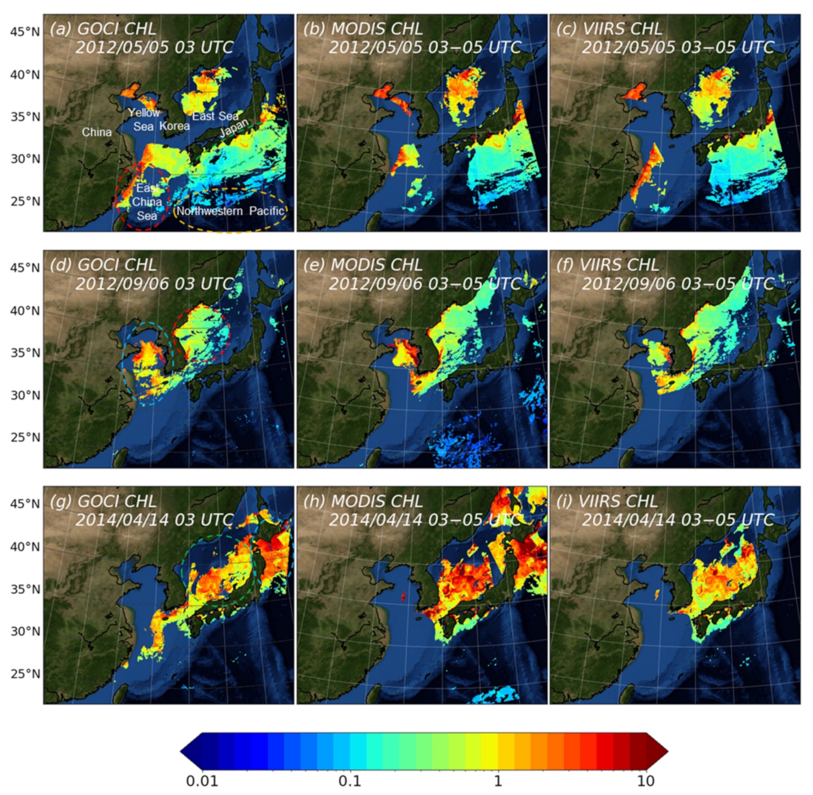
3.1. Scene-by-Scene Comparison among the Three Satellites

This subsection begins with a scene-by-scene comparison among the three satellites for the selected less cloudy days in Figure 1. This comparison demonstrates the advantage of the geostationary ocean color sensor, as the GOCI data obtained at only 03 UTC include a more extensive and more continuous Chl-a observation area than the MODIS and VIIRS data accumulated for three hours (03–05 UTC). Three satellite observations on 5 May 2012 (Figure 1a–c) widely capture the world’s most turbid and dynamic ocean waters interacting with river discharge over the East China Sea (Figure 1a–c) and the Yellow Sea (Figure 1d–f), spring blooms over the East Sea (Figure 1a–c,g–i), and the most transparent water over the subtropical Northwestern Pacific (Figure 1a–c). Overall, the GOCI Chl-a reasonably corresponds with the MODIS and VIIRS to capture consistent marine biological distributions in the qualitative sense. Typical swirls seen in all of the ocean color images (green circles in Figure 1a,g) may be due to the instability of warm ocean currents (Kuroshio current and East Korea Warm Current) intruding off the southern coast of Japan and the East Sea, respectively [32].
The consistency among the qualitative Chl-a distribution data is evident on the second selected day (Figure 1d–f). All data capture the increasing phytoplankton biomass caused by a cold-water upwelling event near Pohang on Korea’s east coast (compare the red circle of Figure 1d–f). Similarly, on the last selected day (14 April 2014), the GOCI and MODIS data (Figure 1g,h) both reveal massive spring bloom events occurring both over the East Sea (the green circle in Figure 1g) and over the Oyashio region south of Hokkaido (blue circle in Figure 1g). However, the VIIRS orbit missed the latter event. We also found some discrepancies among the satellite data in the phytoplankton biomass. Overall, larger Chl-a values from the MODIS than those from GOCI are notable for spring bloom events over the East Sea and the Yellow Sea. By contrast, the VIIRS minus GOCI differences seem to vary region by region.
One of the significant issues with GOCI data is severe ISRD due to sensor optics generating stray light from various optical paths. Despite adopting the ISRD corrected radiometric data by [24], some artificial discontinuity for slot pairs with North-South alignment (latitudes approximately 42°N) still remains in the GOCI Chl-a image (Figure 1a). Another issue with the GOCI data is adopting a stricter strategy to mask unrealistic GOCI level 2 values given a more challenging geostationary satellite environment (e.g., more frequent pixels with a higher satellite zenith angle). More pixels were masked over the subtropical North Pacific with the GOCI than the MODIS (Figure 1d,g).

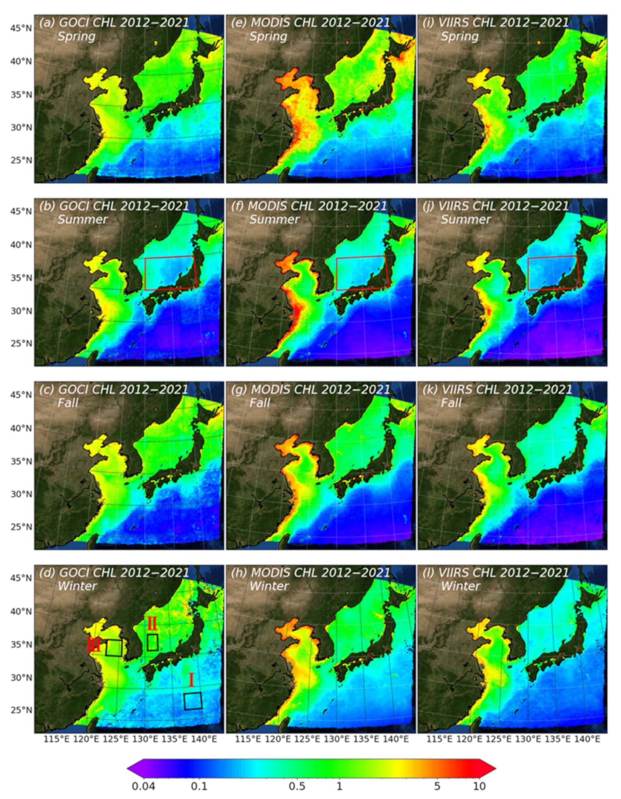
3.2. Climatological Distribution of Phytoplankton Biomass

We extend the analysis period into the concurrent overlapping ocean color mission period (2012–2021). Figure 2 shows the annual mean of the binned GOCI level 2 ocean color data together with those from MODIS and VIIRS (a–c). Here, it would be intriguing to perform an inter-satellite comparison of how the MODIS and VIIRS ocean color data derived from the globally representative database correlate with the GOCI, which is a more regionally representative database.
Notably, the distinct contrast of phytoplankton biomass (between the blue and sky blue color shadings in Figure 2a–c) commonly appears in all three satellites. A sharp S-shaped gradient line exists between the clear waters of Chl-a concentrations below 1.0 mg m−3 (130–140°E, 25–30°N) and the remaining ocean waters in the northwestward direction with higher Chl-a. The location of the distinct Chl-a gradient approximately corresponds with the climatological location of the Kuroshio current. As in [33], the Kuroshio warm current accompanies thermal instability and subsequent intense upwelling north of the current axis, which provides a high number of nutrients from the subsurface water and increases phytoplankton productivity.
All data reveal the regional minimum phytoplankton biomass in the southeastern part of the domain. This deep ocean water of the subtropical western Pacific is oligotrophic with a weak supply of new nutrients. Here, phytoplankton is a predominant optical constituent, and it usually covaries with suspended particulate matter (SPM) and colored dissolved organic matter (CDOM). For these Case I waters, the typical blue-green ratio methodology has been somewhat accurate for estimating Chl-a [29]. The Chl-a range from the three data is reasonable for the subtropical western Pacific. However, the VIIRS minimum value (~0.04; Figure 2c) tends to be underestimated relative to the others (Figure 2a,b) over the East Sea and the Yellow Sea. In addition, Figure 2a exhibits some artificial Chl-a noise by the ISRD between the South-North aligned slots in the annual mean, which is evident off the south coast of Japan at approximately 29°N (e.g., between slot 10 and slot 13).
Each satellite data point reveals that the most productive water occurs over the East China Sea and the Bohai Sea. The East China Sea borders the Yangtze River, one of the major global rivers. The Yangtze River discharge introduces a significant amount of terrestrial suspended matter and organic carbon into the ocean. Different data similarly capture the maximum Chl-a zone extending several hundred kilometers, but the difference in the magnitudes of Chl-a is remarkable. The MODIS reveals maximum Chl-a values >5 mg m−3, reaching approximately 300 km from the coast (Figure 2b). Such a high Chl-a zone is relatively narrow for VIIRS (Figure 2c) and hardly seen for GOCI (Figure 2a). Over Case II water, phytoplankton do not solely dominate the optical properties due to the overlapping and uncorrelated absorptions by CDOM and SPM in the blue region of the spectrum [34]. Accordingly, significant differences among the satellites (e.g., MODIS overestimation) may be partly explained by significant uncertainties in the OCx algorithm in highly turbid sediment-dominated waters.
In contrast, good agreement between the MODIS and GOCI data is noticeable over the East Sea. The VIIRS Chl-a values tend to be underestimated compared with both MODIS and GOCI, and a similar bias occurs over the subtropical western North Pacific. The East Sea is a small semi-enclosed marginal sea similar to the open ocean but is also influenced by diverse warm and cold ocean current systems. Due to vertical upwelling and seasonal blooms [35], the water over the East Sea is moderately productive, with area-averaged (130–137°E, 36–41°N) Chl-a values of approximately 0.68, 0.65, and 0.35 mg m−3 for GOCI, MODIS, and VIIRS, respectively.
The three annual distributions of phytoplankton biomass reasonably reveal the major marine biophysical environmental features over Northeast Asian waters (Figure 2a–c). The relative frequency distribution of the annual averaged Chl-a values (Supplementary Figure S1) indicates that MODIS has a more widespread distribution. Except for the values >3 mg m−3, the GOCI and MODIS have similar frequency distribution, with double peaks around 0.05 and 0.5 mg m−3. Some inter-satellite discrepancies in the magnitude of Chl-a exist, but they vary regionally in terms of the characteristics of ocean optical compositions.

3.3. Seasonal Variation

Due to the distinct seasonal variation in ocean environments (warm currents and upwelling water) and atmospheric environments (aerosol and winds) in Northeast Asia, the inter-satellite comparison results can also vary across seasonal time scales. Spring and fall phytoplankton blooms are well known to be a primary seasonal cycle of the East Sea, as in [32]. For VIIRS, the Chl-a peak in spring tends to be slightly more extensive than that in fall (Figure 3i vs. Figure 3k), while the peaks in the two seasons are somewhat similar for the GOCI (Figure 3a vs. Figure 3c). In addition, the overestimation of the speckles of the MODIS Chl-a values (Figure 3e) is apparent in springtime off the west coast of Tohoku and the surrounding waters of Hokkaido. Such discrepancy does not occur in the other seasons. Interestingly, the excellent agreement among the three satellites is remarkable in summer (red box in Figure 3b,f,j). Focusing on the East Sea in Figure 4, we found more productive waters in the western part than in the east adjacent to Japan. In particular, the GOCI agrees with the MODIS (CORR = 0.86) rather than the VIIRS (CORR = 0.85) over the East Sea in summer.
Over the East China Sea, the MODIS and VIIRS data exhibit more prominent Chl-a seasonal peaks in spring and summer than in fall and winter (Figure 3e–h vs. Figure 3i–l). Over the waters around the Yangtze River, the MODIS overestimation of Chl-a relative to the other satellites (as in Figure 2b) is evident for all of the seasons and is remarkable in spring. In contrast, the GOCI (Figure 3a–d) underestimates the Chl-a values overall throughout the seasons, resulting in much decreased seasonal variation in phytoplankton biomass.
The subtropical western North Pacific is located in the dynamic periphery of the subtropical anticyclonic gyre with the world’s most oligotrophic waters with minimal Chl-a concentration [36]. The three ocean color datasets consistently reveal the maximum Chl-a in winter and the minimum Chl-a in summer over the subtropical western North Pacific. The summer expansion and winter contraction within the gyre in the Pacific Ocean [37] may explain the seasonal variation in the most oligotrophic region. As in the annual mean (Figure 2a), the GOCI ISRD biases still remain. The CIDUM [21] significantly alleviated the ISRD biases in summer and fall (Supplementary Figure S2). However, they are the most serious in spring and winter (Figure 3d). Additionally, VIIRS Chl-a underestimation occurs throughout the four seasons (Figure 3i–l).
Overall, the inter-satellite discrepancies also vary seasonally. The GOCI reveals the smallest seasonal perturbation over the East China Sea. All data show the best agreement in the seasonal cycle over the subtropical western North Pacific. A significant inter-satellite discrepancy in the seasonal variation appears over the East Sea, owing to the remarkable MODIS overestimation in the spring season.

3.4. Two-Dimensional Frequency Distribution of Chlorophyll-a and Inter-Comparison Statistics

This section will perform a quantitative inter-comparison of Chl-a products from the MODIS and VIIRS to the corresponding GOCI Chl-a as a reference. In Figure 3d, we focus on three selected areas with contrasting water optical properties: I: Case I-subtropical Western Pacific (WP), II: Case I-East Sea (ES), III: Case II-Yellow Sea (YS). Note that we choose the boxed regions in Figure 3d to avoid the GOCI IRSD issues. We chose two Case I water regions, but “Case I-ES” represent much more productive waters than “Case I: WP”. The Case II-YS is a representative of Case II water condition whose optical properties are primarily determined by mineral particles, CDOM, or microbubbles.
Figure 5 the MODIS and VIIRS Chl-a products versus GOCI Chl-a products are compared based on the two-dimensional contoured frequency analysis diagram (CFAD as in [38]) of individual 2-km monthly binning data in four different seasons, linear regression analyses, and calculating statistical metrics for data inter-comparison (Section 2.3). Here, we only focus on Case II-YS, where the most significant inter-satellite discrepancy occurs within our analysis domain.
Overall, the overestimation of the MODIS Chl-a in spring (Figure 5a) is predominant for the GOCI Chl-a range from 1 to 3 mg m−3, showing the major frequency distribution of the corresponding MODIS Chl-a ranging from 1 to 5 mg m−3. In the linear relationship (Y = 0.94X + 0.95, where X and Y are GOCI and MODIS Chl-a, respectively), disagreement exists due to significant intercept values (0.95), with the largest MAE (1.03) and MAPE (61.52%) values among 8 panels. In contrast, good correspondence is observed in summer (Figure 5b) for the significant frequency ranges (102.5 frequencies for GOCI Chl-a range from 0 to 1.5 mg m−3). The correlation among the two datasets is the highest, and the RMSE, MAE, and MAPE are the lowest in summer throughout all seasons, with a slope of approximately one and an offset value of approximately 0 in the linear relationship (Y = 1.23X − 0.22).
The fall-to-winter comparison between the MODIS and GOCI reveal two major frequency groups divided into “V-shaped” CFADs (Figure 5c,d). Remarkably, this “V-shaped” frequency distribution exists similarly in the VIIRS versus the GOCI CFADs (Figure 5g,h). The common, abnormal frequency distributions in the CFADs from the MODIS and VIIRS to the corresponding GOCI Chl-a products indicate some absolute biases of the reference data. The recumbent frequency group close to the horizontal axis (Figure 5c,g) indicates overestimation of the GOCI Chl-a compared with the comparison target. The GOCI speckles due to inhomogeneous pixels may be physically responsible for these biases. Each GOCI spectral band is obtained at a different acquisition time by delaying the filter wheel rotation. Fast-moving clouds or aerosols often result in misregistered pixels for different bands that may produce significant errors regarding atmospheric correction and Chl-a estimation [34]. In terms of GOCI observations, a spatially scattered distribution of high aerosol speckles occurs from November to winter [27]. As a result, there may be many issues of overestimating Chl-a in Figure 5c,d,g,h.
Overall, underestimation of the VIIRS Chl-a retrieval relative to the GOCI existed throughout all seasons, with all intercepts smaller than 1 (Figure 5e–h). In spring and summer, contrasting comparison results exist between the MODIS and VIIRS relative to the comparable reference data (e.g., Figure 5a vs. Figure 5e; Figure 5b vs. Figure 5f). The MODIS (VIIRS) tends to overestimate (underestimate) Chl-a values relative to the GOCI. With the identical atmospheric correction algorithm [9] and Chl-a retrieval algorithm [29,30], the differences between MODIS and VIIRS imply the differences attributed to sensor calibration.

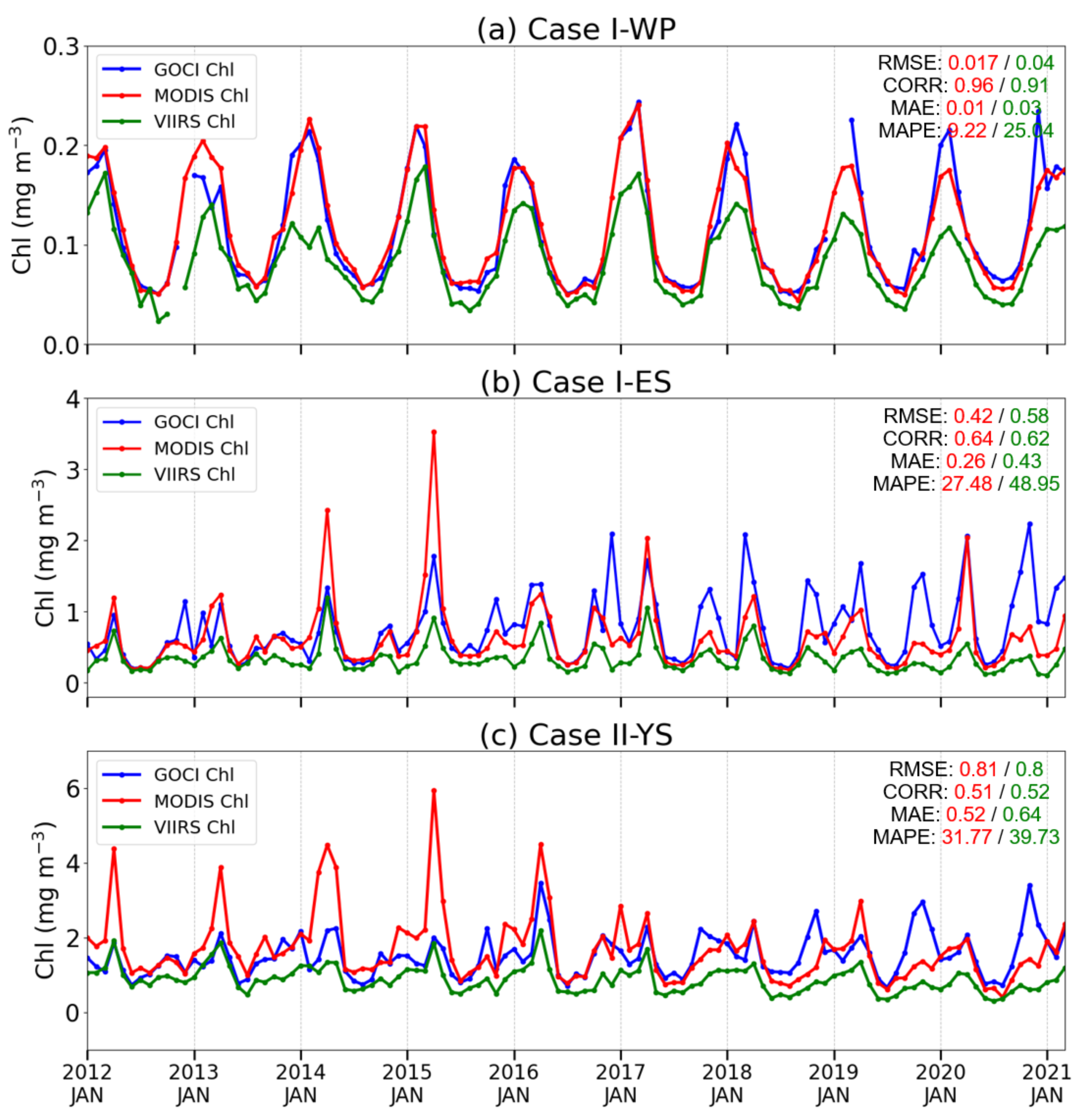
3.5. Inter-Comparison of Chl-a Time Series

This section will investigate whether the abovementioned inter-satellite discrepancies arise for the specified years or the entire period from 2012 to 2021. In Figure 6, we examine the time series of the monthly binned Chl-a data for three selected sites: (a) Case I-WP, (b) Case I-ES, and (c) Case II-YS. In Case I-WP (Figure 6a), the correlations among the three datasets are relatively high (0.91~0.96). However, VIIRS is biased toward lower Chl-a values throughout the entire period (with MAPE = 25.04%). In contrast, the overestimation of MODIS Chl-a at the Case I-ES and Case II-YS sites is not persistent and is somewhat intermittent for specific periods. These discrepancies are only conspicuous in spring 2014 and 2015 for Case I-ES (Figure 6b) and March–April in 2012–2015 for Case II-YS (Figure 6c).
Last, it is noteworthy that the GOCI reveals contrasting inter-satellite discrepancies between the earlier and later (2019–2021) mission periods, particularly for the Case I-ES site. We perform linear regression analysis of the Chl-a monthly time-series (Figure 6b), removing the climatological seasonal cycle. The GOCI reveals an increasing trend in Chl-a values (+0.48 mg m−3 per 9 years during 2012–2020), whereas the MODIS and VIIRS have negative trends (−0.09 and −0.08 mg m−3 per 9 years). The logarithm transforms of the GOCI Chl-a result in the same positive sign but a smaller increasing trend, +0.24 mg m−3 per 9 years. The trend analysis of the National Oceanic and Atmospheric Administration (NOAA) Optimal Interpolation Sea Surface Temperature (OISST) shows that the SST for the Case I-ES site increases by +1.2 K per 9 years. Accordingly, the decreasing Chl-a trends for both the MODIS and VIIRS must be natural marine ecosystem changes in response to ocean warming. The positive Chl-a trends of the GOCI imply the possibility of GOCI sensor degradation in its late mission period.
As in the seasonal distribution, the time-series analysis reveals good consistency among the three satellite data for the entire period, particularly in Case I-WP (CORRGOCI&MODIS ~0.96; CORRGOCI&VIIRS ~0.91). Over more productive waters, they are less consistent: CORRGOCI&MODIS is approximately 0.64 for Cast I-ES and 0.51 for Case II-YS, owing to the striking spring peaks of the MODIS and the late mission increasing tendency of the GOCI.

4. Discussion

Given the lack of a regular in situ optic measurement network over the ocean, stable agreement among (at least) two satellite datasets provides the reliability of ocean color processing procedures that were independently observed and processed. The results in Section 4 reveal the general consistency among the three ocean color data: generally good correlation over the western North Pacific in all seasons and over the East Sea, particularly in summer.
However, each ocean color sensor reveals at least one particular Chl-a discrepancy that differs from the two other data: (i) VIIRS underestimation over the East Sea and the western North Pacific; (ii) MODIS overestimation over the Yellow Sea and the East Sea; and (iii) GOCI increasing trends in the late mission period. This section discusses possible reasons behind a particular sensor bias in the qualitative sense by investigating the time series of Rrs (Section 4.1) and the inter-satellite dependencies as a function of atmospheric quality or water quality (Section 4.2).

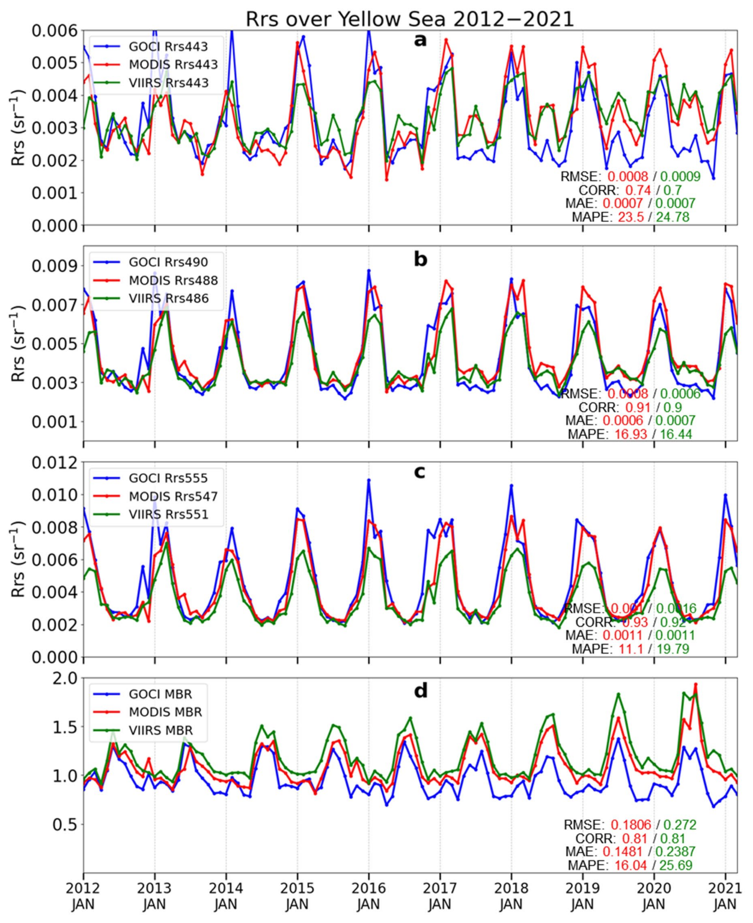
4.1. Multi-Year Time Series of Rrs and Blue to Green Band Ratio

Differences among the three satellites can occur at various steps, such as inherent sensor issues, different atmospheric algorithms, and different Chl-a algorithms. As summarized in Table 3, the GOCI applied the different OC3 coefficients [22] that differed from those of the MODIS and VIIRS Chl-a algorithms [29]. It remains unclear whether Chl-a discrepancies originate from differences in the Chl-a algorithms or the earlier steps. Figure 7, Figure 8 and Figure 9 show the time series of Rrs at the three bands and the maximum blue to green band ratio (MBR) used for the Chl-a estimation (Table 3). The spectral bands of the three satellites are not identical, as shown in Table 1. The blue and green bands for the Chl-a OC3 band-ratio algorithms are 443, 490, and 555 nm for GOCI; 443, 488, and 547 nm for MODIS; and 443, 486, and 551 nm for VIIRS.
First, the systematic underestimation of VIIRS Chl-a relative to MODIS and GOCI occurs over the western North Pacific and the East Sea from the annual and seasonal means (Figure 2 and Figure 3). This systematic difference occurs persistently in the time series throughout the entire analysis period (Figure 6). Large VIIRS blue to green band ratios (MBRs) relative to the MODIS occur consistently for all three selected regions (Figure 7d, Figure 8d and Figure 9d). In particular, the VIIRS 551 nm band’s underestimation relative to the MODIS 547 nm band is notable (Figure 7c, Figure 8c and Figure 9c). Wu et al. [35] performed an inter-comparison of the VIIRS and MODIS calibrations using vicarious approaches. They revealed a negative difference in VIIRS minus MODIS green band radiances both for the selected simultaneous nadir overpasses and desert pixels, which corresponds with the current inter-satellite differences in East Asian seas. Therefore, the inherent sensor calibration issue of the VIIRS and MODIS green bands are responsible for the Chl-a difference, despite using identical atmospheric correction and Chl-a retrieval procedures.
Second, overestimating MODIS Chl-a magnitudes relative to others is evident over the East China Sea and the Yellow Sea, both in the annual and seasonal means (Section 3.2 and Section 3.3). Such a discrepancy only occurs in spring in specific years: 2014–2015 for Case I-ES (Figure 6b) and 2012–2015 for Case II-YS (Figure 6c). Notably, the MODIS episodic (2012, 2013, 2014) overestimation relative to the GOCI (Figure 6c) is attributed to similar MBR values (Figure 9d). This finding indicates that different Chl-a algorithm coefficients impact the Chl-a differences. For example, the same MBR values (~1.3) in spring 2014 (Figure 9d) can derive two times larger Chl-a values in the MODIS (4.2 mg m−3) compared with the GOCI (2.1 mg m−3) in Figure 6d. However, the most prominent 2015 spring MODIS overestimation peak is attributed to the underestimated peaks in the MODIS Rrs in the blue bands (443 nm and 488 nm) compared with the other satellites. In this case, uncertainties both from inherent sensor characteristics and atmospheric correction procedures led to the MODIS’s striking peaks.
Last, the artificial increasing trend of the GOCI (Figure 6) corresponds with the decreasing MBR trends (Figure 7, Figure 8 and Figure 9d). The linear regression analysis of the time series indicates that the GOCI MBR tends to decrease: −0.0011 per 9 years for Case I-ES. However, the MODIS and VIIRS MBR values increase by +0.006 and +0.0009 per 9 years, respectively. The decreasing Rrs trends of the GOCI are evident for the 443 nm and 490 nm bands rather than the 555 nm band. NASA OBPG has put effort into each sensor’s calibration and correction and applied vicarious calibration to stable ground data such as Marine Optical BouY (MOBY) to minimize temporal biases [5]. However, the current GOCI data can have biases due to the sensor’s temporal degradation and the regional characteristics of vicarious calibration sites (Table 2). In addition, the GOCI did not have regular in situ observations like MOBY, where marine-time aerosols purely dominate (Table 2). Therefore, the current NIR inter-calibration process can produce uncertainties in vicarious calibration and atmospheric correction procedures based on the presumed aerosol model. Accordingly, the inconsistent multi-year trends between the GOCI and the well-calibrated MODIS and VIIRS data (443 nm and 490 nm Rrs) imply that sensor calibration correction (or an alternative bias correction algorithm) is required for the next update of GOCI data reprocessing.

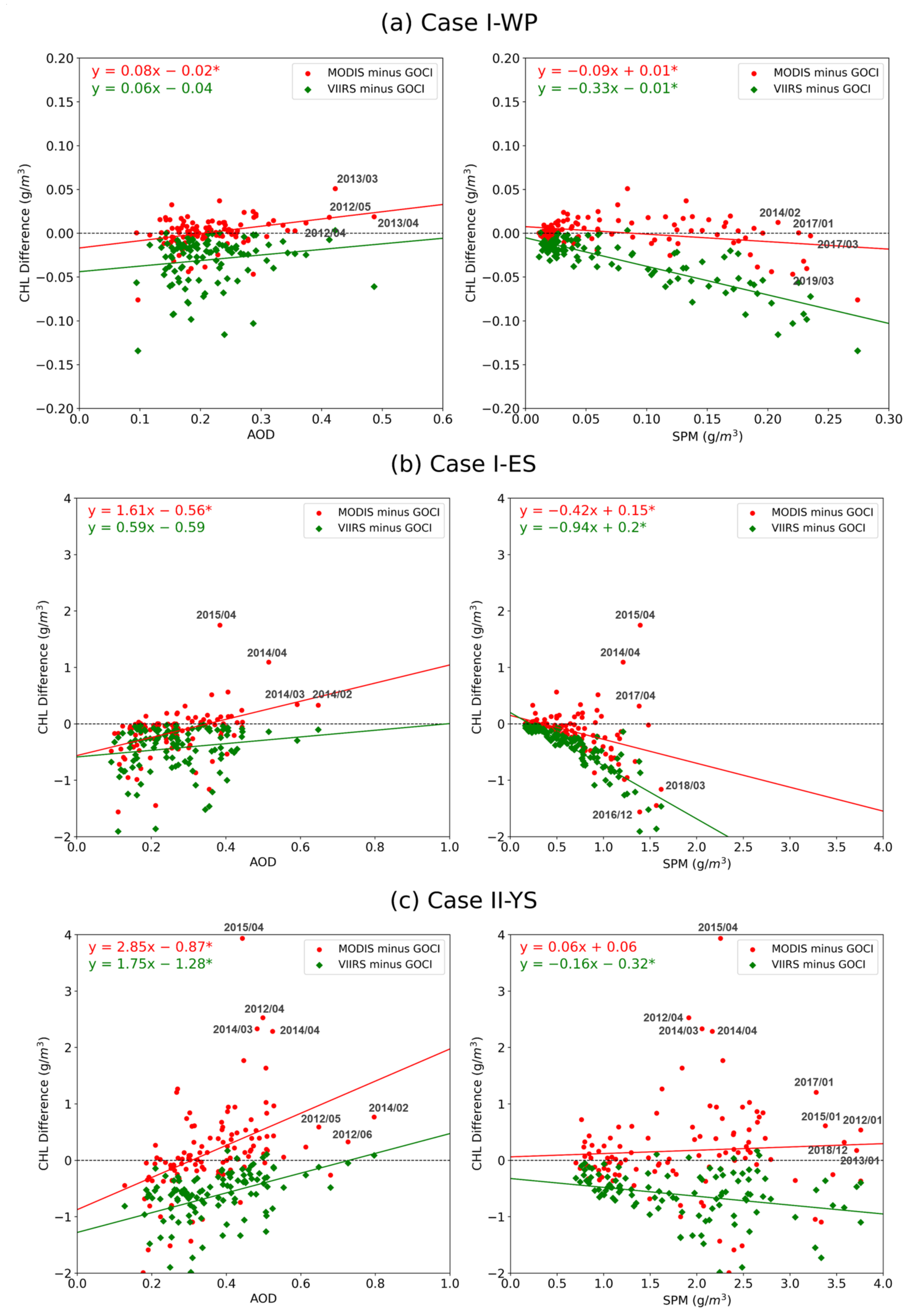
4.2. Inter-Satellite Discrepancy in East Asia’s Dynamic Atmospheric and Ocean Conditions

The current domain encompasses the Yellow Sea, one of the world’s most turbid waters, and the productive East Sea. In addition, East Asia currently has one of the most heavily polluted atmospheres globally, with large anthropogenic emission sources from developing countries and natural aerosol sources from the Gobi deserts and wildfire regions [36]. In Figure 10, we examine inter-satellite Chl-a differences as a function of aerosol optical depth (AOD) and SPM values separately.
Overall, the MODIS˗GOCI Chl-a differences in Figure 10 depend on AOD values, revealing sharper positive regression slopes in Case I-ES (1.61) and Case II-YS (2.85) than in Case I-WP (0.08). The MODIS˗GOCI Chl-a differences cannot be explained solely by water quality conditions since the regression slopes on SPM are not significantly positive for all regions (see right panels in Figure 10). Apparent springtime significant MODIS-GOCI discrepancy events occur under the combined effect of poor aerosol and water quality conditions, as they occur primarily in moderate-to-high SPM and AOD ranges (see left panels of Supplementary Figure S3). For example, the sporadic MODIS overestimation for Case I-ES (Figure 10b) in spring 2014 occurred, with the highest aerosols drifting in the atmosphere (AOD ~ 0.5–0.6) with relatively turbid ocean optical conditions (SPM ~ 1.3). The large inter-satellite difference in 2015 occurred under moderately significant aerosol loading conditions (AOD ~ 0.4) and under more turbid water (SPM ~ 1.5). For Case II-YS, the 2012–2015 springtime with apparent MODIS˗GOCI Chl-a differences reveals moderate-to-high AOD (>0.6 in 2012 and 2014) and SPM (>0.3 in 2013 and 2015) values.
In contrast, the VIIRS˗GOCI Chl-a difference is less dependent on atmospheric aerosol loading (green dots in Figure 10). They show smaller but statistically significant positive slopes (0.59 for Case I-ES and 1.75 for Case II-YS). Instead, the VIIRS-GOCI values rely primarily on SPM with larger negative slopes. Larger VIIRS-GOCI discrepancies are found in more turbid water conditions (see the right panels in Supplementary Figure S3).
The different atmospheric correction (as in Table 2) results between GOCI, VIIRS, and MODIS may be affected by the following factors. First, GOCI atmospheric correction uses Shettle and Fenn’s aerosol models [27], while the VIIRS and MODIS atmospheric correction algorithms use Ahmad’s aerosol models [23]. Second, GOCI’s atmospheric correction scheme determines a best-fit aerosol model in the multiple-scattering domain, while the MODIS-Aqua and VIIRS schemes find a best-fit aerosol model in the single-scattering domain [25].
Different sensor optical characteristics can cause different atmospheric correction results, although vicarious system calibration is applied to all sensors. Notably, the vicarious calibration does not calibrate the longest NIR band gain, assuming that it is already well calibrated. Although the different calibrations of the last NIR band may not cause significantly different atmospheric correction results [37], the difference can be amplified for high aerosol load cases or erroneous aerosol model selection cases. The atmospheric correction algorithms of GOCI, MODIS, and VIIRS select appropriate aerosol models (Table 3) using two NIR wavelengths assuming non or less-absorbing aerosol models. However, yellow dust aerosols, which have strong absorbance characteristics, occur around the Korean Peninsula in spring. This yellow dust’s high aerosol optical thickness and light absorbance characteristics generally cause more significant erroneous aerosol selections during the atmospheric correction process. Amplified aerosol determination errors with each sensor’s different NIR calibration status and characteristics bring different results, although the MODIS and VIIRS employ the same algorithm and aerosol models.
Unrealistic Rrs retrievals may cause a big difference between GOCI and MODIS/VIIRS Chl-a in more turbid waters (Figure 10b,c). To deal with the black pixel assumption over turbid waters, the GOCI uses the regional spectral relationships of water reflectance between red (660 nm) and two NIR wavelengths (745, 865 nm), while MODIS and VIIRS use semi-analytic optical models focusing on global waters. Ahn and Park [39] showed that the semi-analytic approach underestimates NIR water reflectance over GOCI’s observation area compared to the GOCI’s method based on the spectral relationship. Accordingly, we conclude that the challenging East Asian Ocean color environment with atmospheric and ocean optical complexities may invoke significant uncertainties in each sensor’s atmospheric correction procedure, which finally contributed to the inter-satellite difference.

4.3. Seasonal Cycle of Chl-a and Rrs for Low Biomass Region

Recent research by [16] reveals a previously undocumented seasonal bias in Rrs of most polar-orbiting ocean color sensors in the clear water through MOBY evaluation data. Here, we will first compare the seasonal cycle of Rrs from three sensors for Case I whether the GOCI is also biased similarly to the MODIS and VIIRS sensors at low biomass regions.
Case I-WP is located in the dynamic periphery of the subtropical anticyclonic gyre with the world’s most oligotrophic waters with minimal Chl-a concentration [40]. The three ocean color datasets consistently reveal the maximum Chl-a in winter and the minimum Chl-a in summer over the subtropical western North Pacific (Figure 3 and Figure 6a). The summer expansion and winter contraction within the gyre in the Pacific Ocean [40] may explain the seasonal variation in the most oligotrophic region.
For the seasonal cycle of Chl-a at Caes I-WP (Figure 11a), the GOCI reveals the minimum in summer, an increasing trend from November to January, and the maximum in February to March. Due to the significant absorption by phytoplankton biomass from winter to early spring, the Rrs at the blue bands (443 to 490 nm) reveal the minimum (Figure 11b,c). Overall, the GOCI follows the seasonal cycle, with the ocean color satellites consistent with MOBY [16]. The summer peak of MODIS (Figure 11d,e) increases further (e.g., ~7 sr−1 for 488 nm) than GOCI and VIIRS (e.g., ~5.5 sr−1 for GOCI 490 nm and VIIRS 486 nm). However, three data do not agree in the seasonal cycle of Rrs for longer wavelengths (551 to 555 nm). First, the summer-time elevated Rrs seasonal bias [16] is absent for the GOCI (Figure 11c). The GOCI shows the flat Rrs values from spring to fall (March to October), but it reveals the smaller seasonal peak in winter (December to January). By contrast, the MODIS has the primary peak in summer and the secondary in winter (Figure 11f). Finally, the VIIRS reveals the single seasonal peak in spring (Figure 11i).
The bio-geochemical floats (https://biogeochemical-argo.org/data-access.php, [41] (accessed on 1 December 2021)) exit over a region close to the Case I-WP region (September 2018 to March 2019, Supplementary Figure S4; [42]). The Argo observations enable a quick investigation if the satellite observed seasonal evolution is due to natural biogeochemical variability or an artificial signal. For this purpose, a 50 × 50-bin window of the satellite 2-km binning data was selected to match the Argo location. The homogeneous test was performed using the ratio of maximum versus minimum satellite values.
The Argo observation shows stationary Chl-a and bbp in fall, with the increasing trend in winter and the maximum in the early spring, which well represents the climatological seasonal bloom in Figure 3 and Figure 11a. Although the uncertainties in Chl-a exist both in Argo and satellite data, the GOCI well reflects the seasonal phytoplankton bloom in winter to spring (the highest correlation and the lowest RMSE with Argo, Figure 12c). By contrast, the VIIRS is not good at representing the seasonal phytoplankton bloom in this region.
In general, a weak positive relationship between bbp and Rrs (555 nm) is reasonable based on the ocean color model [43]. Based on the positive relationship between ARGO bbp and GOCI Rrs (555) (Supplementary Figure S4b), we assume that the GOCI seasonal cycle may reflect natural bio-geochemical seasonal variation. However, interpreting the inter-satellite difference in the seasonal cycle of Rrs (555) should be carefully concluded in future studies; a more in-depth investigation is necessary to clarify the causes of the GOCI seasonal cycles.

5. Summary and Conclusions

This study presents the current status of the consistency and stability of the world’s first decadal record of geostationary ocean color measurements, the GOCI. We perform an assessment of the multi-year GOCI level 2 data through comparison with the well-calibrated MODIS and VIIRS data. Since its launch in 2010, the GOCI data have been mainly evaluated using in situ ocean biological and optics measurements over the East Asian Marginal Seas [20,22]. Applying hourly varying GOCI data has been beneficial to ocean environmental monitoring at short-term scales, such as red tides [18], floating algae blooms [44], and the resuspension of particles by tidal effects [17]. As the subsequent satellite, GOCI-II loaded on Geo-Kompsat-2A was launched in February 2020 and planned for use until 2030. Multi-mission geostationary ocean color data over the complex bio-optical waters of the East Asian region will accumulate for the next 20 years. At this point, the GOCI must obtain the most accurate decadal record, which is consistent with the long-term calibrated ocean color records. In this aspect, we examined the first multi-year analyses of the level 2 GOCI data using the new atmospheric algorithm [21], the regional OC3 algorithm [22], and the CIDUM [24].
This study shows the inter-satellite comparison results among the three satellite datasets with diverse metrics from individual snap-shots, annual to seasonal climatology, two-dimensional frequency distribution, multi-year time series (Section 3), and scatter plots (Section 4.2). The GOCI Chl-a is retrieved based on the independent atmospheric correction algorithm and the regionally specified Chl-a algorithm, which differs from the MODIS and VIIRS for global ocean applications. The GOCI processing methodology was designed for the complex ocean and atmospheric optical conditions in East Asia. By applying the different methodologies to different sensors, it is not easy to attribute the inter-satellite discrepancies to a particular sensor, as discussed in [45]. The differences in sensor calibration are difficult to detangle quantitatively from differences in atmospheric correction and Chl-a retrieval procedures. However, statistical consistencies among at least two data points provide a valuable tool to confirm the reliability of two ocean color processing procedures that were independently observed and processed.
In general, the current results reveal the consistency between the GOCI and the polar-orbiting ocean color data in the annual and seasonal climatology (Section 4.2 and Section 4.3). The GOCI corresponds well with MODIS and VIIRS in the annual and seasonal patterns of Chl-a, implying the possibility of climatological application. The GOCI reasonably represents the major biological patterns (Section 3.2): the oligotrophic waters over the northwestern Pacific, the sharp gradient of Chl-a along the Kuroshio current, the productive waters over the East Sea, and the highly turbid and productive waters over the East China Sea and the Yellow Sea. During the seasonal cycle (Section 3.3), three satellites commonly reveal double peaks (spring and fall phytoplankton blooms) over the East Sea, spring to summer peaks over the East China Sea, and winter peaks over the western North Pacific, despite some inter-satellite differences in the seasonal cycle of Chl-a magnitude. Additionally, good inter-satellite agreement is remarkable for western North Pacific waters (Figure 6a and Figure 7), which confirms the reliability of GOCI, MODIS, and VIIRS ocean color retrievals for oligotrophic water environments. Even for the productive water environment over the East Sea, the particularly good agreement among the three data points in summer is quite remarkable (Figure 4a vs. Figure 4b).
Given East Asia’s diverse ocean optical complexities and springtime aerosol-rich environments, the three ocean color satellite datasets reveal individual sensor discrepancies that differ from others (Figure 8). First, the VIIRS reveals the systematic underestimation of Chl-a relative to the MODIS and GOCI. The inherent sensor calibration issue of the VIIRS green band is responsible for the systematic inter-satellite discrepancy. Second, the sporadic springtime Chl-a peaks in the MODIS relative to the GOCI and VIIRS may be related to the increasing uncertainties in atmospheric correction procedures in turbid water conditions under aerosol-rich environments.
The GOCI Rrs at 555 nm does not reveal the seasonal bias as in the other ocean color data for low biomass waters [16]. In contrast to the summer peak in the MODIS and VIIRS, the GOCI shows the flat Rrs values from spring to fall (March to October), with the seasonal peak in winter. Based on the similar winter peaks in Argo bbp, the GOCI seasonal cycle may properly represent the bio-geochemical seasonal cycle.
This study also reveals the current limitation of the GOCI data, which requires further improvement. The GOCI sensor degradation effect in the late mission period on Chl-a retrieval will be presented in a separate paper. Planned adjustments to GOCI calibration (2022) in the following GOCI-II data will essentially eliminate this positive bias in Chl-a trends. Adopting the CIDUM procedure [24] significantly lessened the ISRD errors. See Supplementary Figure S2 for the advancement in the seasonal variation in GOCI Chl-a by applying the CIDUM. The remaining GOCI ISRD errors will be corrected based on the artificial intelligence technique.
The current results highlight that inter-satellite comparison metrics can provide a useful test to confirm the reliability of a sensor’s ocean color data. Franz et al. [5] analyzed the sixteen-year SeaWiFS-MODIS-VIIRS time series to investigate the consistent behavior between MODIS and VIIRS Chl-a in 2013 owing to the radiometric performance of the VIIRS. Investigating the inter-satellite data finally leads to a reprocessing of the VIIRS data, leading to a more accurate time series.
The GOCI algorithms had been developed and validated for optically complex environments (e.g., turbid water, seasonal phytoplankton bloom, and seasonal dust). The multi-year GOCI time series without temporal bias will be valuable for understanding the ecological impact of global warming and other anthropogenic changes on this region [3]. In particular, the East Asian Marginal Seas are known to be one of the world’s most rapidly warming ocean regions [46]. At this time, the long-term application of the GOCI data should be made with the caveat to diagnose the ecological impacts or validate ocean ecosystem modeling. Therefore, the current methodology for coherency and inconsistency among the various ocean color missions will be adopted to determine near-real-time GOCI and GOCI-II data for future capabilities and the directions of long-term ocean monitoring applications. However, planned temporal adjustments to GOCI calibration (2022) in the following GOCI-II satellite will essentially eliminate the bias in Chl-a trends.

Supplementary Materials

The following are available online at https://www.mdpi.com/article/10.3390/rs14010072/s1, Figure S1: Figure 1. Histogram (relative frequency) of annual mean Chl-a values (Figure 2) of GOCI, MODIS, and VIIRS from Figure 2. Figure S2: The ISRD improved GOCI Chl-a, as shown in Figure 3, after applying the CIDUM procedure (left panels) in comparison with those before CIDUM (right panels). Figure S3: Inter-satellite discrepancies (shading, color bar on the right) as a function of SPM on the x-axis and AOD on the y-axis: MODIS minus GOCI difference (in left panels) and VIIRS minus GOCI difference (in right panels) for (a) Case I-WP, (b) Case I-ES and (c) Case II-YS.

Author Contributions

Conceptualization: M.-S.P.; methodology: M.-S.P., S.L., S.-J.L. and J.-H.A.; software: M.-S.P. and S.L.; investigation, M.-S.P., S.L., S.-J.L. and J.-H.A.; data curation: S.-J.L.; writing—original draft preparation, M.-S.P.; writing—review and editing, J.-H.A., J.-K.C. and J.-H.R.; visualization: S.L.; funding acquisition: M.-S.P. and J.-H.R. All authors have read and agreed to the published version of the manuscript.

Funding

This research was supported by the “Operation of the Korea Ocean Satellite Center” funded by KIOST, and the “Technology development for Practical Applications of Multi-Satellite data to maritime issues” funded by the Ministry of Ocean and Fisheries, Korea.

Informed Consent Statement

Not applicable.

Data Availability Statement

Note that the GOCI L1B data are available at the KIOST KOSC homepage at http://kosc.kiost.ac.kr (accessed on 1 December 2021), and the data with the ISRD correction will be officially provided soon. To produce Rrs and Chl-a, the GDPS2.0 software downloaded at http://kosc.kiost.ac.kr (accessed on 1 December 2021) is applied. The MODIS and VIIRS level 2 Chl-a and Rrs data are available from the NASA OBPG website at https://oceandata.sci.gsfc.nasa.gov/ (accessed on 1 December 2021). The Argo data are available from the biogeochemical Argo website at https://biogeochemical-argo.org/data-access.php/ (accessed on 1 December 2021).

Acknowledgments

We sincerely appreciate the editor and three anonymous reviewers for their valuable comments and suggestions. In particular, the suggestions by the second reviewer have significantly improved the quality of this paper. The first author thanks Young-Je Park in KOSC, KIOST for his scientific encouragement of this study. The authors also thank NASA and NOAA for operating the MODIS and VIIRS missions. We thank the NASA Goddard Space Flight Center (the Ocean Ecology Laboratory and Ocean Biology Processing Group) for providing the processed MODIS and VIIRS level 2 data.

Conflicts of Interest

The authors declare no conflict of interest.

References

  1. Behrenfeld, M.J.; Randerson, J.T.; McClain, C.R.; Feldman, G.C.; Los, S.O.; Tucker, C.J.; Falkowski, P.G.; Field, C.B.; Frouin, R.; Esaias, W.E.; et al. Biospheric Primary Production During an ENSO Transition. Science 2001, 291, 2594–2597. [Google Scholar] [CrossRef] [Green Version]
  2. Field, C.B.; Behrenfeld, M.J.; Randerson, J.T.; Falkowski, P. Primary production of the biosphere: Integrating terrestrial and oceanic components. Science 1998, 281, 237–240. [Google Scholar] [CrossRef] [Green Version]
  3. Behrenfeld, M.J.; O’Malley, R.T.; Siegel, D.A.; McClain, C.R.; Sarmiento, J.L.; Feldman, G.C.; Milligan, A.J.; Falkowski, P.G.; Letelier, R.M.; Boss, E.S. Climate-driven trends in contemporary ocean productivity. Nature 2006, 444, 752–755. [Google Scholar] [CrossRef]
  4. Dutkiewicz, S.; Hickman, A.E.; Jahn, O.; Henson, S.; Beaulieu, C.; Monier, E. Ocean colour signature of climate change. Nat. Commun. 2019, 10, 578. [Google Scholar] [CrossRef] [PubMed] [Green Version]
  5. Franz, B.A.; Bailey, S.W.; Meister, G.; Werdell, P.J. Quality and consistency of the NASA ocean color data record. In Proceedings of the Ocean Optics XXI, Glasgow, UK, 8–12 October 2012. [Google Scholar]
  6. Eplee, R.E.; Meister, G.; Patt, F.S.; Barnes, R.A.; Bailey, S.W.; Franz, B.A.; McClain, C.R. On-orbit calibration of SeaWiFS. Appl. Opt. 2012, 51, 8702–8730. [Google Scholar] [CrossRef] [PubMed]
  7. Eplee, R.E.; Turpie, K.R.; Meister, G.; Patt, F.S.; Fireman, G.F.; Franz, B.A.; McClain, C.R. A Synthesis of VIIRS Solar and Lunar Calibrations. Earth Obs. Syst. XVIII 2013, 8866, 88661L. [Google Scholar] [CrossRef] [Green Version]
  8. Franz, B.A.; Bailey, S.W.; Werdell, P.J.; McClain, C.R. Sensor-independent approach to the vicarious calibration of satellite ocean color radiometry. Appl. Opt. 2007, 46, 5068–5082. [Google Scholar] [CrossRef]
  9. Gordon, H.R.; Wang, M. Retrieval of water-leaving radiance and aerosol optical thickness over the oceans with SeaWiFS: A preliminary algorithm. Appl. Opt. 1994, 33, 443–452. [Google Scholar] [CrossRef]
  10. Zibordi, G.; Mélin, F.; Berthon, J.F.; Talone, M. In situ autonomous optical radiometry measurements for satellite ocean color validation in the Western Black Sea. Ocean Sci. 2015, 11, 275–286. [Google Scholar] [CrossRef] [Green Version]
  11. Wang, M.; Gordon, H.R. A simple, moderately accurate, atmospheric correction algorithm for SeaWiFS. Remote Sens. Environ. 1994, 50, 231–239. [Google Scholar] [CrossRef]
  12. Wang, M.; Son, S.H. VIIRS-derived chlorophyll-a using the ocean color index method. Remote Sens. Environ. 2016, 182, 141–149. [Google Scholar] [CrossRef]
  13. Brickley, P.J.; Thomas, A.C. Satellite-measured seasonal and inter-annual chlorophyll variability in the Northeast Pacific and Coastal Gulf of Alaska. Deep Sea Res. Part II Top. Stud. Oceanogr. 2004, 51, 229–245. [Google Scholar] [CrossRef]
  14. Hu, C.; Muller-Karger, F.E.; Taylor, C.; Carder, K.L.; Kelble, C.; Johns, E.; Heil, C.A. Red tide detection and tracing using MODIS fluorescence data: A regional example in SW Florida coastal waters. Remote Sens. Environ. 2005, 97, 311–321. [Google Scholar] [CrossRef]
  15. Hu, C. A novel ocean color index to detect floating algae in the global oceans. Remote Sens. Environ. 2009, 113, 2118–2129. [Google Scholar] [CrossRef]
  16. Bisson, K.M.; Boss, E.; Werdell, P.J.; Ibrahim, A.; Frouin, R.; Behrenfeld, M.J. Seasonal bias in global ocean color observations. Appl. Opt. 2021, 60, 6978–6988. [Google Scholar] [CrossRef]
  17. Hoi, J.-K.; Park, Y.J.; Ahn, J.H.; Lim, H.-S.; Eom, J.; Ryu, J.-H.; Choi, C.; Park, Y.J.; Ahn, J.H.; Lim, H.-S.; et al. GOCI, the world’s first geostationary ocean color observation satellite, for the monitoring of temporal variability in coastal water turbidity. J. Geophys. Res. Ocean. 2012, 117, 9004. [Google Scholar] [CrossRef]
  18. Noh, J.H.; Kim, W.; Son, S.H.; Ahn, J.H.; Park, Y.J. Remote quantification of Cochlodinium polykrikoides blooms occurring in the East Sea using geostationary ocean color imager (GOCI). Harmful Algae 2018, 73, 129–137. [Google Scholar] [CrossRef] [PubMed]
  19. Doxaran, D.; Lamquin, N.; Park, Y.J.; Mazeran, C.; Ryu, J.H.; Wang, M.; Poteau, A. Retrieval of the seawater reflectance for suspended solids monitoring in the East China Sea using MODIS, MERIS and GOCI satellite data. Remote Sens. Environ. 2014, 146, 36–48. [Google Scholar] [CrossRef]
  20. Moon, J.E.; Park, Y.J.; Ryu, J.H.; Choi, J.K.; Ahn, J.H.; Min, J.E.; Son, Y.B.; Lee, S.J.; Han, H.J.; Ahn, Y.H. Initial validation of GOCI water products against in situ data collected around Korean peninsula for 2010–2011. Ocean Sci. J. 2012, 47, 261–277. [Google Scholar] [CrossRef]
  21. Ahn, J.; Park, Y.; Kim, W.; Lee, B.; Gordon, H.R.; Brown, J.W.; Evans, R.H. Simple aerosol correction technique based on the spectral relationships of the aerosol multiple-scattering reflectances for atmospheric correction over the oceans. Opt. Express 2016, 24, 29659–29669. [Google Scholar] [CrossRef]
  22. Kim, W.; Moon, J.E.; Park, Y.; Ishizaka, J. Evaluation of chlorophyll retrievals from Geostationary Ocean Color Imager (GOCI) for the North-East Asian region. Remote Sens. Environ. 2016, 184, 482–495. [Google Scholar] [CrossRef]
  23. Ahmad, Z.; Franz, B.A.; McClain, C.R.; Kwiatkowska, E.J.; Werdell, J.; Shettle, E.P.; Holben, B.N. New aerosol models for the retrieval of aerosol optical thickness and normalized water-leaving radiances from the SeaWiFS and MODIS sensors over coastal regions and open oceans. Appl. Opt. 2010, 49, 5545–5560. [Google Scholar] [CrossRef]
  24. Kim, W.; Ahn, J.H.; Park, Y.J. Correction of Stray-Light-Driven Interslot Radiometric Discrepancy (ISRD) Present in Radiometric Products of Geostationary Ocean Color Imager (GOCI). IEEE Trans. Geosci. Remote Sens. 2015, 53, 5458–5472. [Google Scholar] [CrossRef]
  25. Ahn, J.H.; Park, Y.J.; Ryu, J.H.; Lee, B.; Oh, I.S. Development of atmospheric correction algorithm for Geostationary Ocean Color Imager (GOCI). Ocean Sci. J. 2012, 47, 247–259. [Google Scholar] [CrossRef]
  26. Ahn, J.-H.; Park, Y.-J.; Kim, W.; Lee, B.; Oh, I.S. Vicarious calibration of the Geostationary Ocean Color Imager. Opt. Express 2015, 23, 23236–23258. [Google Scholar] [CrossRef]
  27. Shettle, E.P.; Fenn, R.W. Models for the Aerosols of the Lower Atmosphere and the Effects of Humidity Variations on Their Optical Properties; Air Force Geophysics Laboratory, Air Force Systems Command, United States Air Force: Montgomery County, OH, USA, 1979. [Google Scholar]
  28. Bailey, S.W.; Franz, B.A.; Werdell, P.J. Estimation of near-infrared water-leaving reflectance for satellite ocean color data processing. Opt. Express 2010, 18, 7521–7527. [Google Scholar] [CrossRef] [PubMed]
  29. O’Reilly, J.E.; Maritorena, S.; Mitchell, B.G.; Siegel, D.A.; Carder, K.L.; Garver, S.A.; Kahru, M.; McClain, C. Ocean color chlorophyll algorithms for SeaWiFS. J. Geophys. Res. Ocean. 1998, 103, 24937–24953. [Google Scholar] [CrossRef] [Green Version]
  30. Hu, C.; Lee, Z.; Franz, B. Chlorophyll aalgorithms for oligotrophic oceans: A novel approach based on three-band reflectance difference. J. Geophys. Res. Ocean. 2012, 117, 1011. [Google Scholar] [CrossRef] [Green Version]
  31. IOCCG. Guide to the Creation and Use of Ocean-Colour, Level-3, Binned Data Products; Antoine, D., Ed.; Reports of the International Ocean-Colour Coordinating Group, No. 4; International Ocean-Colour Coordinating Group (IOCCG): Dartmouth, NS, Canada, 2004; 88p. [Google Scholar] [CrossRef]
  32. Kim, S.W.; Saitoh, S.I.; Ishizaka, J.; Isoda, Y.; Kishino, M. Temporal and Spatial Variability of Phytoplankton Pigment Concentrations in the Japan Sea Derived from CZCS Images. J. Oceanogr. 2000, 56, 527–538. [Google Scholar] [CrossRef]
  33. MIYASHITA, M. Bi-weekly to Seasonal Variability of Satellite-derived Chlorophyll a Distribution: Controlling Factors in the Ocean South of Honshu Island. J. Remote Sens. Soc. Japan 2005, 25, 169–178. [Google Scholar] [CrossRef]
  34. Moses, W.J.; Gitelson, A.A.; Berdnikov, S.; Povazhnyy, V. Estimation of chlorophyll-a concentration in case II waters using MODIS and MERIS data—successes and challenges. Environ. Res. Lett. 2009, 4, 45005. [Google Scholar] [CrossRef] [Green Version]
  35. Wu, A.; Mu, Q.; Angal, A.; Xiong, X. Assessment of MODIS and VIIRS calibration consistency for reflective solar bands calibration using vicarious approaches. In Proceedings of the Sensors, Systems, and Next-Generation Satellites XXIV, online, 21–25 September 2020; Volume 11530, p. 1153018. [Google Scholar]
  36. Choi, M.; Lim, H.; Kim, J.; Lee, S.; Eck, T.T.; Holben, B.B.; Garay, M.J.; Hyer, E.E.; Saide, P.P.; Liu, H. Validation, comparison, and integration of GOCI, AHI, MODIS, MISR, and VIIRS aerosol optical depth over East Asia during the 2016 KORUS-AQ campaign. Atmos. Meas. Tech. 2019, 12, 4619–4641. [Google Scholar] [CrossRef] [Green Version]
  37. Wang, M.; Gordon, H.R. Calibration of ocean color scanners: How much error is acceptable in the near infrared? Remote Sens. Environ. 2002, 82, 497–504. [Google Scholar] [CrossRef]
  38. Park, M.-S.; Choi, Y.-S.; Ho, C.-H.; Sui, C.-H.; Park, S.K.; Ahn, M.-H. Regional cloud characteristics over the tropical northwestern Pacific as revealed by Tropical Rainfall Measuring Mission (TRMM) Precipitation Radar and TRMM Microwave Imager. J. Geophys. Res. Atmos. 2007, 112. [Google Scholar] [CrossRef] [Green Version]
  39. Ahn, J.-H.; Park, Y.-J.; Fukushima, H. Comparison of Aerosol Reflectance Correction Schemes Using Two Near-Infrared Wavelengths for Ocean Color Data Processing. Remote Sens. 2018, 10, 1791. [Google Scholar] [CrossRef] [Green Version]
  40. Morel, A.; Claustre, H.; Gentili, B. The most oligotrophic subtropical zones of the global ocean: Similarities and differences in terms of chlorophyll and yellow substance. Biogeosciences 2010, 7, 3139–3151. [Google Scholar] [CrossRef] [Green Version]
  41. Bisson, K.M.; Boss, E.; Westberry, T.K.; Behrenfeld, M.J. Evaluating satellite estimates of particulate backscatter in the global open ocean using autonomous profiling floats. Opt. Express 2019, 27, 30191–30203. [Google Scholar] [CrossRef]
  42. Wang, T.; Chen, F.; Zhang, S.; Pan, J.; Devlin, A.T.; Ning, H.; Zeng, W. Remote Sensing and Argo Float Observations Reveal Physical Processes Initiating a Winter-Spring Phytoplankton Bloom South of the Kuroshio Current Near Shikoku. Remote Sens. 2020, 12, 4065. [Google Scholar] [CrossRef]
  43. Stramska, M.; Stramski, D.; Hapter, R.; Kaczmarek, S.; Stoń, J. Bio-optical relationships and ocean color algorithms for the north polar region of the Atlantic. J. Geophys. Res. Ocean. 2003, 108, 3143. [Google Scholar] [CrossRef] [Green Version]
  44. Son, Y.B.; Choi, B.-J.; Kim, Y.H.; Park, Y.-G. Tracing floating green algae blooms in the Yellow Sea and the East China Sea using GOCI satellite data and Lagrangian transport simulations. Remote Sens. Environ. 2015, 156, 21–33. [Google Scholar] [CrossRef]
  45. Mikelsons, K.; Wang, M.; Jiang, L. Statistical evaluation of satellite ocean color data retrievals. Remote Sens. Environ. 2020, 237, 111601. [Google Scholar] [CrossRef]
  46. Lee, S.; Park, M.-S.; Kwon, M.; Kim, Y.H.; Park, Y.-G. Two major modes of East Asian marine heatwaves. Environ. Res. Lett. 2020, 15, 74008. [Google Scholar] [CrossRef]
Figure 1. Chl-a images from the GOCI (left), MODIS-Aqua (center), and VIIRS (right) on 5 September 2012 (ac), 6 September 2012 (df), and 14 April 2014 (gi). The GOCI 03 UTC image is compared with the MODIS and VIIRS images including all overpasses available between 03–05 UTC. The names of regional seas and countries for this study are printed (a). Major ocean color variabilities are indicated with dashed elliptical circles of different colors.
Remotesensing 14 00072 g001
Figure 2. Annual mean Chl-a concentrations from the (a) GOCI, (b) MODIS, and (c) VIIRS averaged from January 2012 to March 2021.
Remotesensing 14 00072 g002
Figure 3. Seasonal (spring, summer, fall, and winter) distribution of Chl-a concentrations from the GOCI (left), MODIS (center), and VIIRS (right) from 2012 to 2021. In panel d, three representative study areas with distinctive optical properties: “I: Case I-subtropical Western Pacific (WP)”, “II: Case I-East Sea (ES)”, and “III: Case II-Yellow Sea (YS)”.
Remotesensing 14 00072 g003
Figure 4. Enlarged images of summer-mean distribution of Chl-a concentrations over the East/Japan Sea from the GOCI, MODIS, and VIIRS.
Remotesensing 14 00072 g004
Figure 5. Two-dimensional contoured frequency analysis diagram (CFAD) of the MODIS versus GOCI Chl-24a (left panels) and those of the VIIRS versus GOCI Chl-a concentrations (right panels) over the Case II-Yellow Sea region: spring (a,e), summer (b,f), fall (c,g), and winter (d,h). Linear regression analysis (y = a x + b) and statistical metrics (RMSE, CORR, MAE, and MAPE) are shown at the right-upper corner.
Remotesensing 14 00072 g005
Figure 6. Time series of chlorophyll-a concentrations for the GOCI (blue), MODIS (red), and VIIRS (green) in the selected areas of (a) Case I-subtropical Western Pacific (WP), (b) Case I-East Sea (ES), and (c) Case II-Yellow Sea (YS), as shown in Figure 3d. The inter-comparison statistics between MODIS (VIIRS) and GOCI are in a red (green) font at the upper-right corner.
Remotesensing 14 00072 g006
Figure 7. Time series (2012–2021) of remote sensing reflectances (Rrs) for the GOCI, MODIS, and VIIRS in the selected area of the subtropical Western Pacific in the (a) blue #1, (b) blue #2, and (c) green bands, and (d) maximum ratio of blue to green bands (MBR).
Remotesensing 14 00072 g007
Figure 8. Same as Figure 7 except for the time series of Rrs in the selected East Sea area.
Remotesensing 14 00072 g008
Figure 9. Same as Figure 7 except for the time series of Rrs in the selected Yellow Sea area.
Remotesensing 14 00072 g009
Figure 10. Scatterplots of inter-satellite Chl-a differences (MODIS-GOCI for red; VIIRS-GOCI for green) versus aerosol optical depth (AOD) in the left panels or suspended particular matter (SPM) in the right panels from the GOCI: Case I-WP, Case I-ES, and Case II-YS. The linear regression analysis results with slopes and intercepts between the Chl-a differences and AOD (SPM) are in the upper left corner of the left (right) panels. * indicate significant value with a 95% confidence level.
Remotesensing 14 00072 g010
Figure 11. Seasonal averages of Chl-a and Rrs with error bars from (ad) GOCI, (eh) MODIS, and (il) VIIRS for Case I-WP. Note that the wavelength of each sensor is slightly different. The error bars indicate the standard errors of the monthly binning Chl-a data.
Remotesensing 14 00072 g011
Figure 12. Time series of (a) Chl-a and (b) bbp (700) from September 2018 to March 2019 from WMO Argo #2902750 observation (with location in Supplementary Figure S4). (c) Scatter plots between Argo versus satellite-derived Chl-a values for fall (September to November in small filled circles) and winter and spring (from December to March in large-filled circles) with the statistics. Note that Argo was processed using Quality Flag information, and unrealistic outlines are removed using a 3× standard deviation threshold. Chl-a is averaged over 0–20 m depth, and bbp is averaged in the euphotic depth (0~200 m) [42].
Remotesensing 14 00072 g012
Table 1. Comparison of the sensor characteristics of the three ocean color satellites, GOCI/COMS, MODIS/Aqua, and VIIRS/NPP.
GOCI/COMSMODIS/AquaVIIRS/NPP
Mission lifeJune 2010–present2002–resentOctober 2011–present
Horizontal resolution (m)500 m1 km750 m
Observational time
over Northeast Asia
8 times a day
00 UTC–08 UTC
03–05 UTC03–05 UTC
Spectral bands
in nm
(1) 412, (2) 443, (3) 490,
(4) 555, (5) 660, (6) 680,
(7) 745, (8) 865
(8) 415, (9) 443, (10) 490, (11) 531, (12) 565, (13) 653, (14) 681, (15) 750, (16) 865(1) 412, (2) 445, (3) 488,
(4) 555, (5) 672, (6) 746,
(7) 865
Table 2. Major methodologies in the atmospheric correction (AC), vicarious calibration, and sensor calibration of the three satellite datasets.
GOCIMODIS and VIIRS
AC candidate
aerosol models
Maritime, coastal, and tropospheric aerosol models with different relative humidity (11 models, [27])Maritime aerosol models with different fine mode fraction and relative humidity (80 models; [23])
AC extrapolation of aerosol reflectance from NIR to VISSpectral relationship of aerosol
multiple-scattering reflection between
different wavelengths [21]
Single scattering reflectance model (epsilon) to convert to multiple-scattering reflectance [9]
AC
NIR turbid water
correction
Empirical relationships of water reflectance between red and two NIR bands [25]Semi-analytic optical model with estimated backscattering and absorption coefficient
[28]
Vicarious
calibration
Using Northwest Pacific for NIR vicarious calibration site
Visible bands calibrated with shipboard
observations of Case I waters around Korea [26]
Using South Pacific Gyre and the Southern
Indian Ocean sites for NIR inter-calibration.
Visible bands calibrated with MOBY data
[8]
on-board calibrationPeriodic solar observations
Temporal correction planned
Periodic lunar and/or solar observations
Temporal correction done in NASA ocean color Data Reprocessing [5,7]
Table 3. Chlorophyll-a (Chl-a) algorithm of the three satellite datasets.
Functional forms of the OCx algorithm log 10 C h l a = C 0 + C 1 log 10 1 X + C 2 log 10 2 X + C 3 log 10 3 X +
C 4 log 10 4 X
XOC3 = max(Rrs(443), Rrs(490))/Rrs(555)
GOCIC0 = 0.0831, C1 = −1.9941, C2 = 0.5629, C3 = 0.2944, C4 = −0.5458
MODIS and VIIRSC0 = 0.2424, C1 = −2.7423, C2 = 1.8017, C3 = 0.0015, C4 = −1.2280
Publisher’s Note: MDPI stays neutral with regard to jurisdictional claims in published maps and institutional affiliations.

