Article

Quantification of the Environmental Impacts of Highway Construction Using Remote Sensing Approach

1
National Engineering Laboratory for Applied Technology of Forestry & Ecology in South China, Central South University of Forestry and Technology (CSUFT), Changsha 410004, China
2
College of Life Science and Technology, Central South University of Forestry and Technology (CSUFT), Changsha 410004, China
3
College of Mechanical and Electronic Engineering, Central South University of Forestry and Technology (CSUFT), Changsha 410004, China
*
Author to whom correspondence should be addressed.
Remote Sens. 2021, 13(7), 1340; https://doi.org/10.3390/rs13071340
Submission received: 10 February 2021 / Revised: 21 March 2021 / Accepted: 29 March 2021 / Published: 1 April 2021
(This article belongs to the Section Environmental Remote Sensing)

Abstract

:
Highways provide key social and economic functions but generate a wide range of environmental consequences that are poorly quantified and understood. Here, we developed a before–during–after control-impact remote sensing (BDACI-RS) approach to quantify the spatial and temporal changes of environmental impacts during and after the construction of the Wujing Highway in China using three buffer zones (0–100 m, 100–500 m, and 500–1000 m). Results showed that land cover composition experienced large changes in the 0–100 m and 100–500 m buffers while that in the 500–1000 m buffer was relatively stable. Vegetation and moisture conditions, indicated by the normalized difference vegetation index (NDVI) and the normalized difference moisture index (NDMI), respectively, demonstrated obvious degradation–recovery trends in the 0–100 m and 100–500 m buffers, while land surface temperature (LST) experienced a progressive increase. The maximal relative changes as annual means of NDVI, NDMI, and LST were about −40%, −60%, and 12%, respectively, in the 0–100m buffer. Although the mean values of NDVI, NDMI, and LST in the 500–1000 m buffer remained relatively stable during the study period, their spatial variabilities increased significantly after highway construction. An integrated environment quality index (EQI) showed that the environmental impact of the highway manifested the most in its close proximity and faded away with distance. Our results showed that the effect distance of the highway was at least 1000 m, demonstrated from the spatial changes of the indicators (both mean and spatial variability). The approach proposed in this study can be readily applied to other regions to quantify the spatial and temporal changes of disturbances of highway systems and subsequent recovery.

1. Introduction

Highways provide key social and economic functions and services to human societies, including transportation, travel, cultural exchange, and flow of materials and information [1,2,3]. At the same time, they generate a wide range of adverse ecological consequences (e.g., habitat destruction, species extinction, landscape fragmentation, and ecosystem degradation) through landscape segmentation, acoustic disturbances, edge effects, and human-aided dispersal of diseases [4,5,6]. The need to understand the spatial and temporal spread of these environment impacts caused by highway is more pressing than ever [7] because of the massive existing road systems and projected large increase in road length in developing countries [8,9,10]. Many studies have demonstrated that highway construction and operation can have diverse landscape and ecological impacts [6,11,12]. The effect distance or road-effect zone, the distance over which significant ecological effects extend outward from a road [11], has been used widely to quantify the ecological impacts of road construction and use [6,13,14,15]. The identification of the road-effect zone is essential to transportation planning and maintenance operations [13]. Various effect distances have been reported, including 1500 m for leopard frog (Rana pipiens) [16], 400 m for desert tortoises (Gopherus agassizii) [17], 250–1000 m for five species of anurans [18], 1300 m for great bustards (Otis tarda) [19], 400 m for land-use types [20], and 2000 m for the vegetation index [14]. It should be realized that the effect distance is variable dependent and therefore multiple effect distances coexist. In addition, the effect distances are asymmetric to a road due to slope, wind, and habitat differences on opposite sides of the road [11,15,20]. Consequently, the road-effect zone is asymmetric to the road and variable longitudinally along the road [14,20]. Defining the longitudinal changes of a road-effect zone makes it possible to estimate the proportion of the land ecologically affected by roads and to identify the critical areas or sections for restoration and protection [21,22]. Despite the usefulness of the road-effect zone it is still very difficult to identify it, mainly because of the need for repetitive sampling in time and space, which is expensive and difficult to achieve.
Understanding the ecological processes in time series are essential for environmental engineering, monitoring, mitigation, and management [23,24]. Thereby, long time series of remotely sensed data have a key role to play as they can capture some aspects of ecosystem changes caused by roads [14,25,26,27]. Gülci et al. (2017) [28] found that approximately 18% of the coniferous forests within a 100-m zone along the road were degraded between 2000 and 2015 using a Landsat-derived normalized difference vegetation index (NDVI). Alphan and Derse [29] analyzed landscape changes in the Mediterranean using NDVI derived from Landsat images and found that forest deforestation occurred at low altitudes in close proximity to roads. However, it is worth mentioning that most of these studies rely on a few cloud-free images every few years, which might not be sufficient to capture the temporal changes of road impacts from construction to operation, let alone minimizing the errors caused by images acquired at different points in time [30,31]. As a result, new remote sensing-based approaches need to be developed to support the monitoring and assessment of highway impacts on the environment.
A detailed understanding of how a highway impacts landscape patterns and ecosystem processes is critical to planners and property managers as they try to mitigate the impacts of highway construction and assist in the restoration of disturbed landscapes [32,33]. The purpose of this study was to develop a new approach using remote sensing images acquired at different points in time to assess the spatial and temporal impacts of highway construction on the environment and the ecological recovery processes. Our objectives were to: (1) develop a new general approach, using remote sensing data across different times for change detection, to quantify environmental impacts of highways; (2) explore the effect distance for ecological indicators along a newly constructed highway; and (3) build an effective environment quality assessment framework for assessing the environmental impacts of highways.

2. Materials and Methods

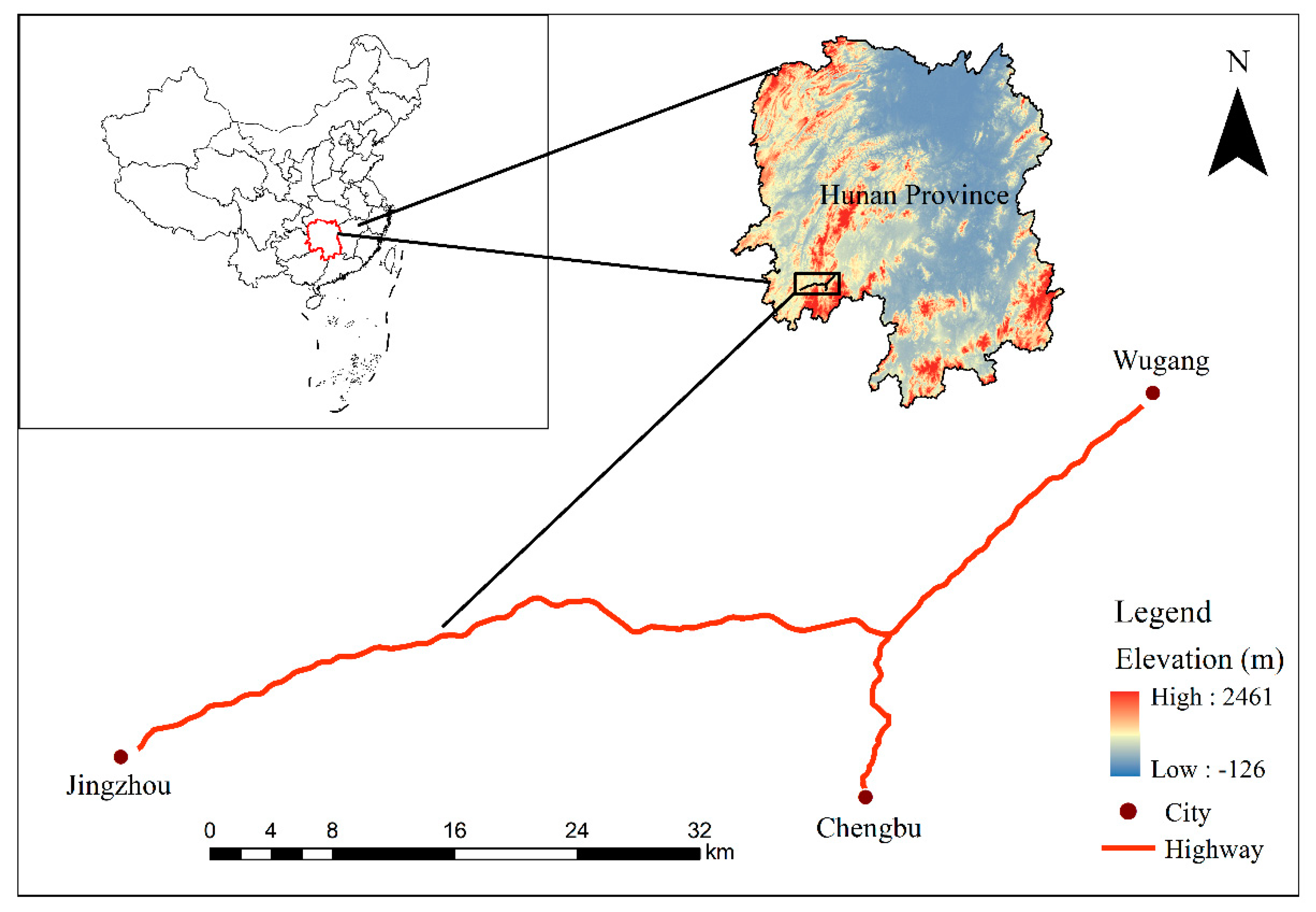
2.1. Study Area and Data Sources

The study site (109°49′–112°57′E, 25°58′–27°40′N) was the Wujing Highway (WJH), a four-lane highway located in the southwest part of Hunan Province, China (Figure 1). The highway stretched for 83 km from the southwest of Wugang City to Jingzhou City, including the main line (72 km) and Chengbu branch line (11 km). WJH construction started in 2013 and was completed at the end of 2017. The region along the highway is typical hilly landform with complex terrain and the highest altitude along the highway is 692 m above sea level. The region has a subtropical climate with the long-term average annual temperature of 16.8 °C. The long-term average annual precipitation is 1218.5 mm, and the monsoon season is from April to July. The land cover of the surrounding areas is mainly composed of agricultural land, forest, water bodies, and smaller villages.
We used a series of Landsat 8 satellite images acquired from 2013 to 2018, downloaded from the Geospatial Data Cloud (http://www.gscloud.cn, accessed on 10 February 2021), to map the spatial and temporal changes of the environmental and ecological factors before, during, and after the WJH construction (Table 1). To retrieve the ecological indicators, the Landsat 8 images at 30 m resolution were acquired from mainly between May and July from 2013 to 2018. Furthermore, the slope data derived from the Shuttle Radar Topography Mission (SRTM) digital elevation model (DEM) at 30 m spatial resolution was downloaded from USGS (https://earthexplorer.usgs.gov/, accessed on 10 February 2021).

2.2. Calculation of Ecological Indicators

The following three indicators were calculated from Landsat images to represent various aspects of the ecological changes along the highway: (1) normalized difference vegetation index, (2) normalized difference moisture index (NDMI), (3) land surface temperature (LST). The methods for deriving these data layers are described below.

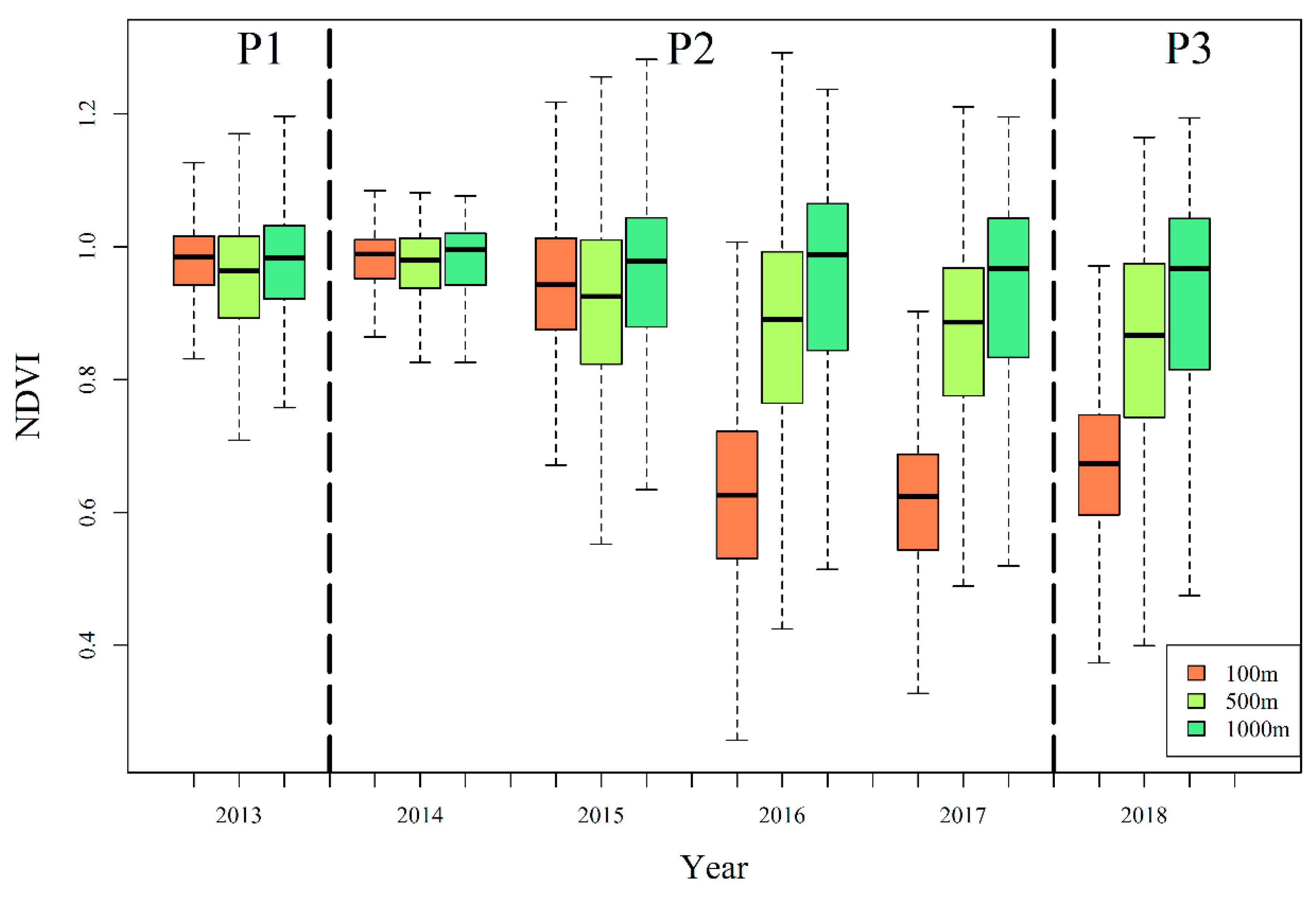
2.2.1. Normalized Difference Vegetation Index

The normalized vegetation index derived from satellites has been frequently used to assess vegetation responses to environmental change in many previous studies [34,35,36]. It is one of the most commonly used vegetation indices for monitoring ecosystem dynamics and processes [37,38]. The NDVI is calculated as follows:
N D V I = ( N I R r e d ) / ( N I R + r e d )
where red and NIR are the spectral reflectance measurements acquired in the red and near-infrared regions, respectively. The NDVI values for vegetation are generally positive, with higher index values being associated with greater green leaf areas and biomass [39].

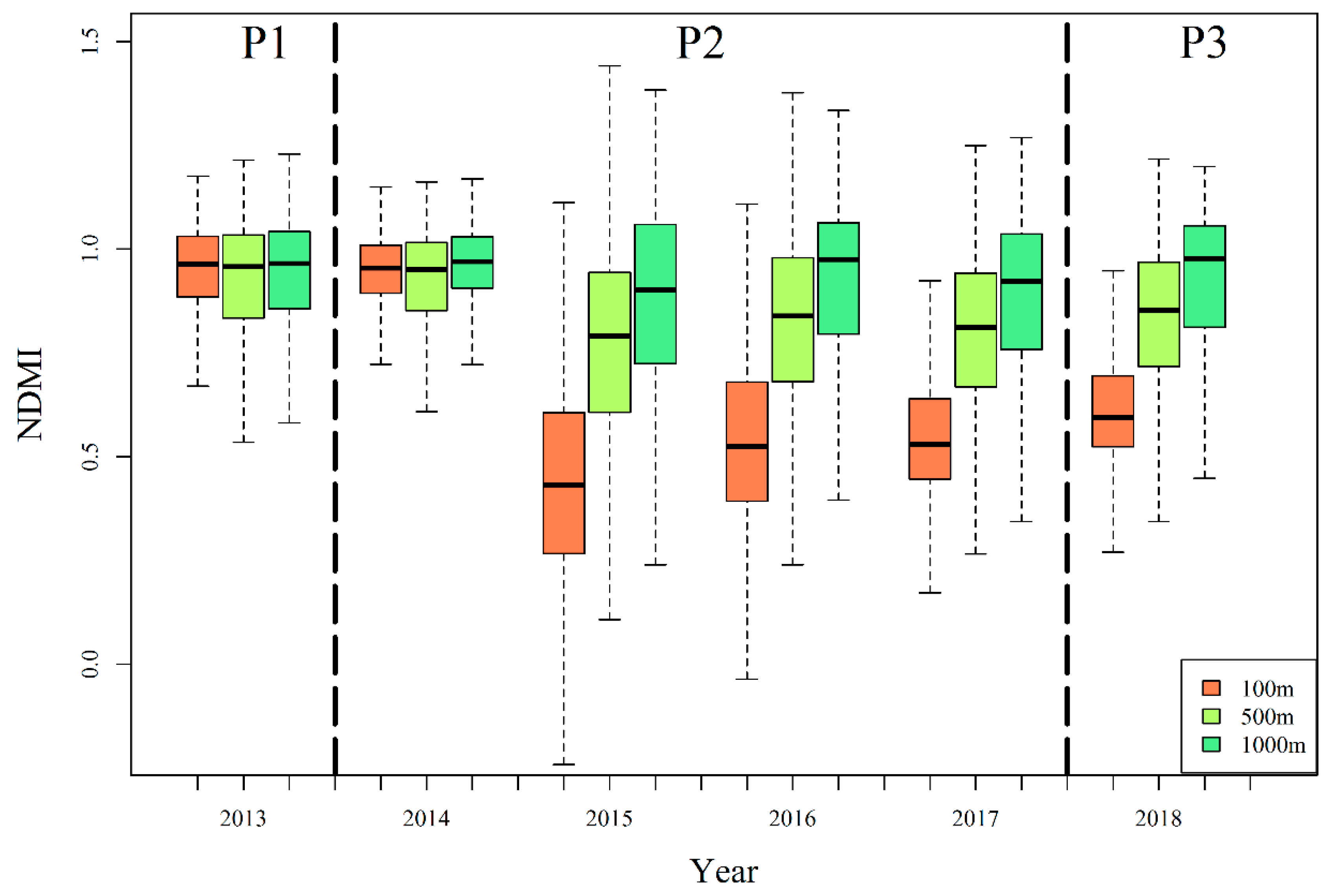
2.2.2. Normalized Difference Moisture Index

Canopy water content is an important indicator of ecosystem stress and health [36]. The normalized difference moisture index is a satellite-derived index that can be calculated from the near-infrared (NIR) and short-wave infrared (SWIR) channels of Landsat [40] as follows:
N D M I = ( N I R S W I R ) / ( N I R + S W I R )
where NIR is the near-infrared band and SWIR is the short-wave infrared band. The NDMI is highly correlated with the water content of canopy [40,41]. The value of NDMI varies from −1 to 1, with larger values indicating greater wetness [42].

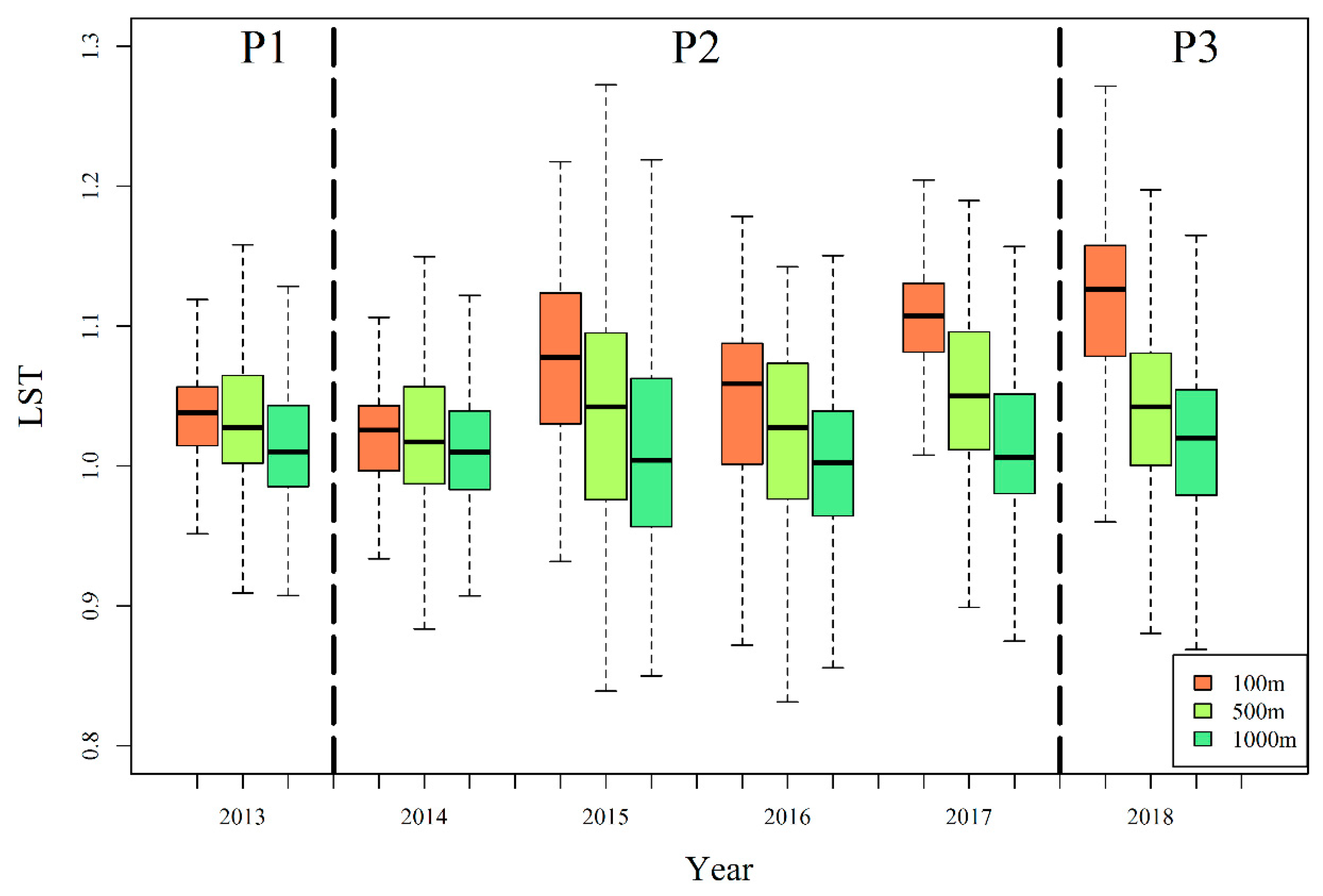
2.2.3. Land Surface Temperature Retrieval

Land surface temperature is an important indicator of ecological conditions that can be derived from remote sensing data [43]. Research on LST shows that the partitioning of sensible and latent heat fluxes and thus surface radiant temperature response is a function of varying surface soil water content and vegetation cover [44,45]. In this study, the information of thermal infrared (TIR) band 10 derived from the Landsat 8 thermal infrared sensor (TIRS) was used to derive the LST using the radiative transfer equation (RTE) [46].
A three-step procedure was adopted to derive the LST [46,47,48]. First, the digital number (DN) of the thermal bands (i.e., bands 10 and 11 in Landsat 8) was converted into to absolute units of at-sensor spectral radiance. Second, the brightness temperature (BT) at each pixel was derived. Finally, the at-sensor brightness temperature was modified to the LST via the varied spectral emissivity depending on real object properties, to reflect the differences in temperature among various cover types on the real land surface.

2.3. Remote Sensing Approach for Assessing Ecological Effects of Highway in Time and Space

Satellite images acquired from the study area captured the spatial and temporal changes of the environment along the highway before, during, and after highway construction realistically. However, these images had to be normalized before they could be used to assess the spatial and temporal changes in environmental conditions since the images were acquired at different points in time which might result in different natural conditions in vegetation and climate [49,50]. As our approach developed in this study was based on the traditional before–during–after control-impact (BDACI) design for collecting field samples to assess the impacts of roads [19,51], we named our approach BDACI remote sensing (BDACI-RS). Specifically, BDACI-RS consists of three major steps: setting buffers along the road, selection of reference or control areas, and normalization of the remote sensing images through time using the reference. These three steps are described below.
The first step was to set buffers along the road. We set the 0–100 m, 100–500 m, and 500–1000 m buffers along the WJH to quantify the effect distance of the highway construction from 2013 to 2018. The maximum buffer of 1000 m was selected following most previous studies, which have shown that effect distances are generally less than 1000 m [52,53,54]. The use of three buffers was to capture the smaller effect distances (<1000 m maximum) along the highway and the possible nonlinear decay of the effects from the highway.
The second step was the selection of reference areas. The reference areas referred to areas that did not experience the impacts of the highway, and they were used as the baseline for change detection in the target area affected by the highway. Two conditions had to be met for the reference areas. First, there had to be no obvious human-induced changes in ecosystem conditions during the entire study period. Second, these reference areas had to have similar soil and climate conditions to the target areas being assessed. These two conditions together ensured that the ecological disparities between the target assessment areas and the reference areas were primarily caused by disturbances, i.e., highway construction in our study. Considering that highway construction can influence the heat balance and vegetation conditions of the landscape surface in the perpendicular direction several kilometers away from the highway [6,14,20,36], a region 5 km away from the highway was selected as the reference area in this study (Figure 2).
The third step was normalization of the ecological conditions in the targeted areas (i.e., the roadside buffers) against those in the reference areas. This was achieved using the following equation, using NDVI as an example:
N D V I n o r m = ( N D V I o b s + 1 ) / ( N D V I m e d i a n , r e f + 1 )
where NDVInorm and NDVIobs are the normalized NDVI and Landsat-derived NDVI, respectively, for the targeted assessment areas, and NDVImedian,ref is the median value of NDVI in the reference areas. We used the median instead of the mean NDVI value to normalize the NDVI in the target areas to avoid the impact of extreme values [55]. Other environmental indicators (e.g., LST and NDMI) were normalized similarly.

2.4. Land Use and Land Cover Classification Using Google Earth Engine

One of the major consequences of highway construction is land use and land cover (LULC) change, especially the transition from natural landscapes to impervious surfaces [56,57]. To explore the impacts of highway construction on LULC change, supervised classification was applied to classify land-cover types along the highway using Google Earth Engine (GEE) (https://earthengine.google.com, accessed on 10 February 2021) following the study by Karan et al. (2016) [40]. The following four data layers were used for LULC classification: the NDVI, the normalized difference built-up index (NDBI), the DEM, and the slope. Four broadly-defined land-cover types, including built-up land, forest, cropland, and water, were classified along the WJH. To set the classification rules, a total of 759 areas of interest (AOIs) were selected as training samples from the Google Earth images along the WJH, including built-up land (203 AOIs), water (102 AOIs), forest (227 AOIs), and cropland (227 AOIs). Additional 300 AOIs for each land-cover type were selected throughout the highway zone to validate the accuracy of classification.

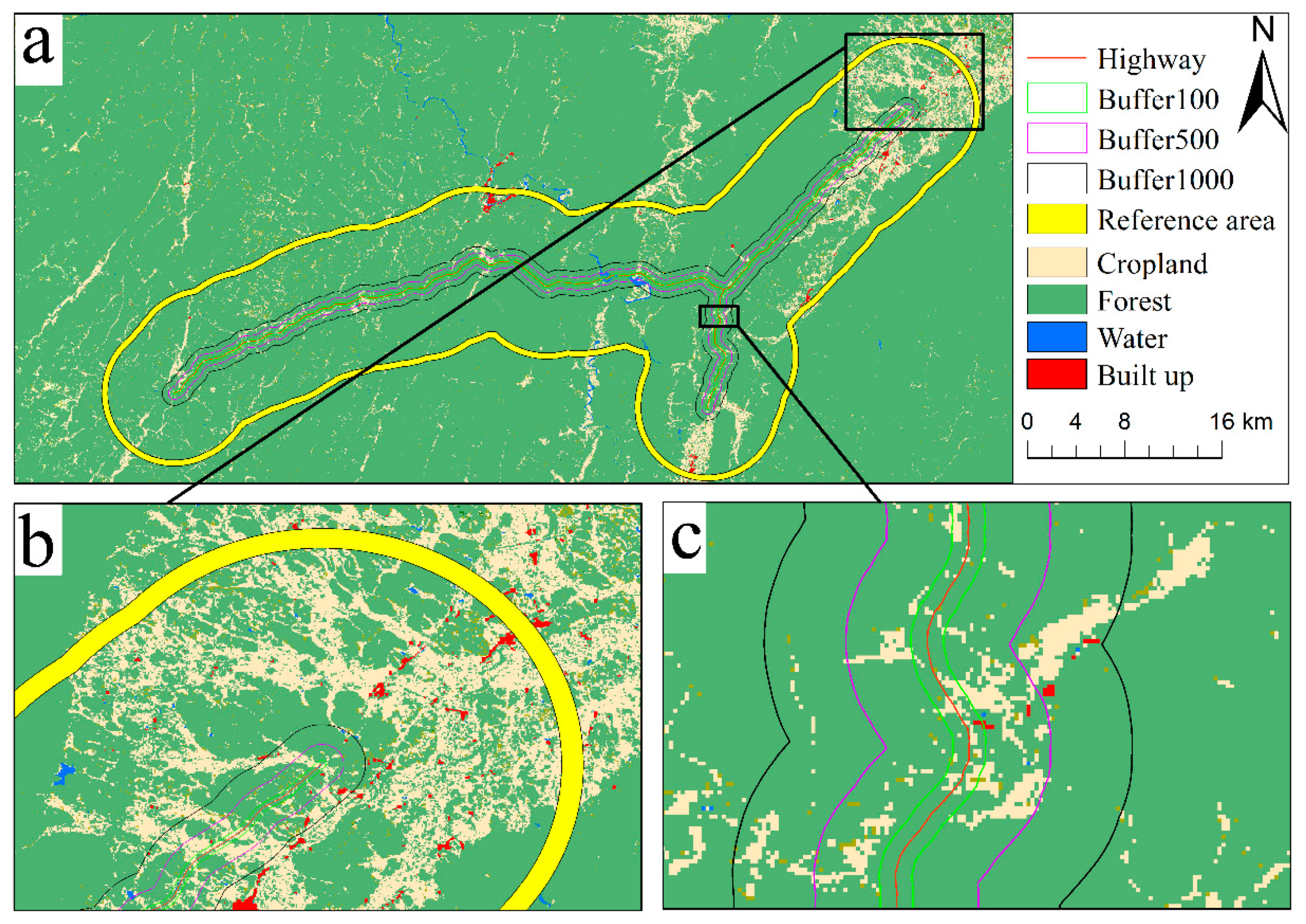
2.5. Identification of the Road-Effect Zone

In general, highway construction affects the region in close proximity the most, and the impact fades away with distance from the highway [18]. To quantify the effect distance of the highway, we examined the changes in LULC and ecological indicators within 0–100 m, 100–500 m, and 500–1000 m buffers on both sides of the highway in ArcGIS 10.2 (ESRI Inc., Redlands, CA, USA). The road-effect zones were quantified in two steps. First, the moving average values of each environmental indicator along the highway in the 0–100 m, 100–500 m, and 500–1000 m zones were calculated to show the location-specific and zone-specific impacts. Second, the location-specific impacts within each zone, calculated above, were summarized, and the temporal changes from 2013 to 2018 were analyzed. These results synoptically show the deterioration and recovery of environmental conditions during and after highway construction in different zones.

2.6. Landscape Patterns

The spatial and temporal changes of landscape patterns can reflect the impact of land use on the ecological environment [58,59,60]. To examine the relationships between landscape changes and highway construction, five indices were selected and calculated to explore the dynamics of the landscape using FRAGSTATS (version 4.2) (Table 2). The percent of landscape (PLAND) provides a general representation of landscape composition, specifically how much of the landscape comprises a particular patch type in a study area [58,61,62]. Patch density (PD) represents the number of patches of a certain type of landscape per spatial unit, reflecting the degree of landscape fragmentation and the density of the patch’s distribution [63]. The edge density (ED) serves as a fundamental index of landscape shape and measures the complexity of the patches [64]. The ED accounts for the length of an edge relative to the area of the patch, and higher ED indicates a more ragged patch [65]. The landscape shape index (LSI) measures the perimeter-to-area ratio for the landscape as a whole and indicates the shape complexity of the landscape [66,67]. The aggregation index (AI) indicates the degree of landscape patch aggregation [68,69].

2.7. Establishment of an Ecological Assessment Model

The construction of highways leads to various changes in ecological conditions [25,70]. To evaluate the overall change, it is necessary to normalize all the ecological metrics as they are in different units or fluctuate within different ranges [27]. The indicators were normalized using the flowing equation:
N i = ( X i X m i n ) / ( X i X m a x )
where Xmin and Xmax are the minimum and maximum of indicator X, respectively, and Ni is the normalized value (ranging from 0 to 1) of the indicator X at pixel i.
Finally, an ecological quality index (EQI) model was built by integrating all the indicators, following previous studies [71,72]:
E Q I i = j = 1 n w j N j , i
where wj and Nj,i, are the weight and normalized value of indicator j for pixel i, respectively. The weights of the indicators, quantifying their relative importance in defining the EQI, were obtained by surveying stakeholders from the government, companies, and land owners, and the results are summarized in Table 3. The ecological quality of a pixel or land parcel was rated as excellent (EQI > 6.5), good (EQI between 5.5 and 6.5), fair (EQI between 4.5 and 5.5), or poor (EQI < 4.5) according to its EQI score, which varied from 0 (worst) to 10 (best).

3. Results

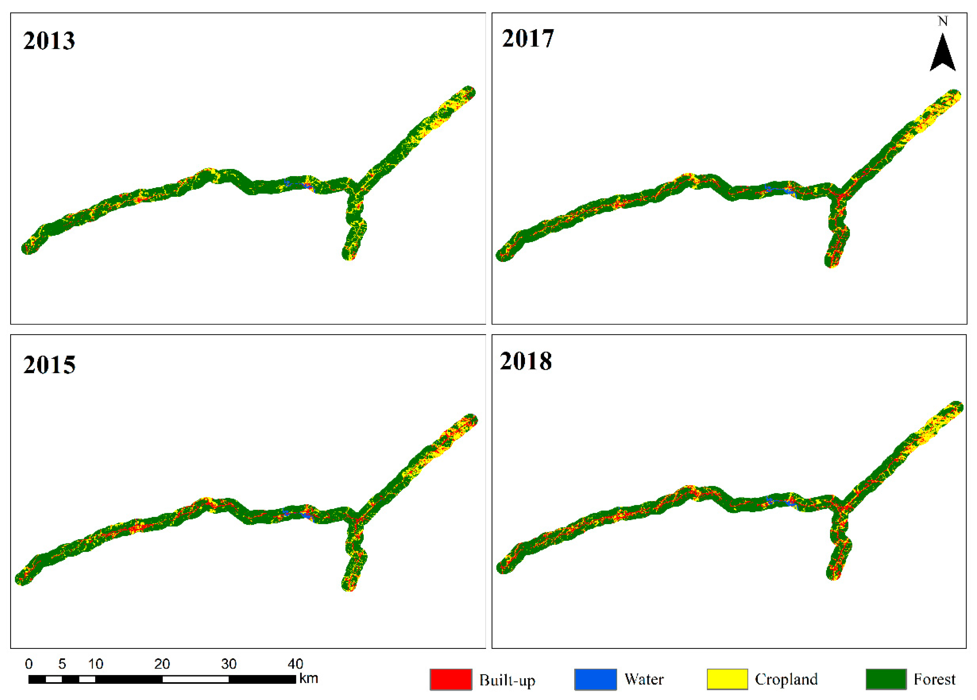
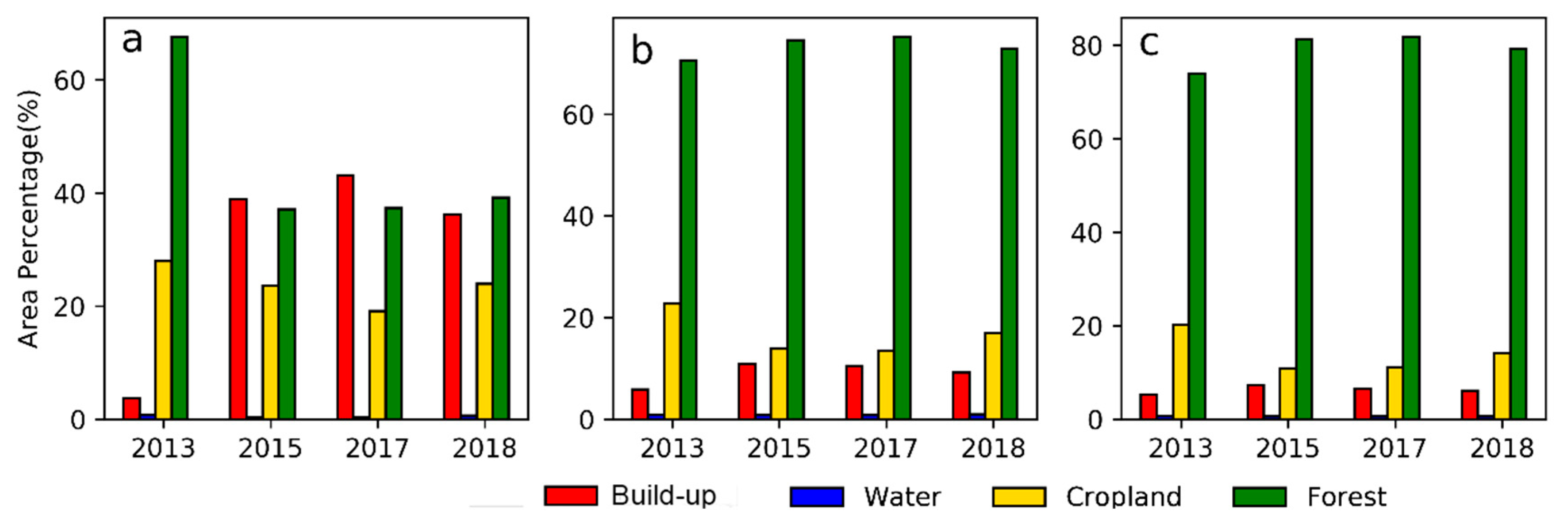
3.1. Impacts of Highway Construction on Land Use/Cover

The maps of major LULC types in 2013, 2015, 2017, and 2018 are shown in Figure 3 and Figure 4. The average overall accuracy of the maps was 85% and the kappa coefficient was 83%, suggesting that the classification was satisfactory [73]. The spatial distribution of LULC types was closely associated with the terrain. The regions with flat terrain were suitable for crop production and traffic networks; thus, these areas were primarily comprised of construction land and cropland. The west section and the north of the Chengbu branch line were mountainous, rugged, and less affected by human activities; therefore, these areas were primarily composed of forest.
The LULC composition along the highway (0–1000 m buffer) experienced substantial change from 2013 to 2018. According to the mapped results, the largest change in LULC was built-up land, which expanded from 7.93 km2 in 2013 to 23.15 km2 in 2018, a net area increase of 15.22 km2 (191.93%). In 2013, about 129.02 km2 (76.52%) of total land area was forest, which shrank to 121.95 km2 (72.31%) in 2015 and further declined to 118.06 km2 (70.00%) in 2018 (Figure 4). The cropland decreased from 30.37 km2 (18.01%) in 2013 to 23.49 km2 (13.93%) in 2017, but this was followed by a rise to 25.84 km2 (15.32%) in 2018. Likewise, water showed a similar trend to cropland, but the magnitude of change in water area was small (0.12%).
Spatially, the LULC compositions in different buffers showed different change intensities during the study period. Before the construction of WJH in 2013, land cover in the 0–100 m buffer was composed of forest, cropland, built-up areas, and water, accounting for 71.80%, 23.90%, 3.50%, and 0.80%, respectively (Figure 4). When construction of the WJH was completed in 2018, the land cover composition in the 0–100 m buffer changed into forest (32.84%), cropland (18.34%), built-up areas (48.06%), and water (0.75%). Overall, in the 0–100 m buffer, forest experienced the largest loss during highway construction, from a coverage of 71.80% to 32.84%; cropland declined from 23.92% to 18.34%; and water remained relatively stable compared with the other three land cover types (Figure 4).
Highway construction also resulted in some LULC changes in the 100–500 m and 500–1000 m buffers as well. In the 100–500 m buffer, the built-up land expanded from 5.20% to 14.20% but the forest area decreased from 74.60% in 2013 to 69.00% in 2018. The expansion of road was mainly at the cost of cropland and forest land, which decreased by 3.50% and 5.60%, respectively. The land cover changes in the 500–1000 m zone basically mimicked the changes seen in the 100–500 m zone, but the built-up land took a small fraction of total area and forest coverage dominated in the total area from 2013 to 2018. The main LULC compositions in the 500–1000 m zone remained relatively stable compared with those in the 0–100 m and 100–500 m zones during the study period (Figure 3).

3.2. Dynamics of Landscape Patterns

The changes of landscape metrics of the 0–1000 m buffer during 2013–2018 are shown in Table 4. The percent of landscape for forest was highest (69.94–76.47) during the study period, followed by cropland (13.94–18.05). The PLAND for water was the lowest (0.76–1.07), showing the sporadic zonal distribution. The PLAND significantly increased in built-up land from 4.07 in 2013 to 13.73 in 2018. The obvious increase of PLAND for built-up land was due to the construction of the highway, which broke the original crop and forest patches, resulting in a more fragmented landscape. Subsequently, the values of the PLAND for cropland and forest land decreased by 2.70 and 6.52, respectively. The patch density obviously increased for built-up land (3.97), cropland (4.59), and forest (0.61) from 2013 to 2018. The PD for water decrease from 0.18 in 2013 to 0.06 in 2018. The evolution of the edge density showed the different degree of the raggedness in land-cover types. The ED for built-up land progressively increased and reached the highest level in 2018. Overall, the ED for cropland and forest land increased by 1.43 and 6.22, respectively, from 2013 to 2018. The LSI of the built-up areas and forest land increased over time, indicating that the landscape patterns experienced drastic changes and the patch shape became increasingly rugged after the highway construction.

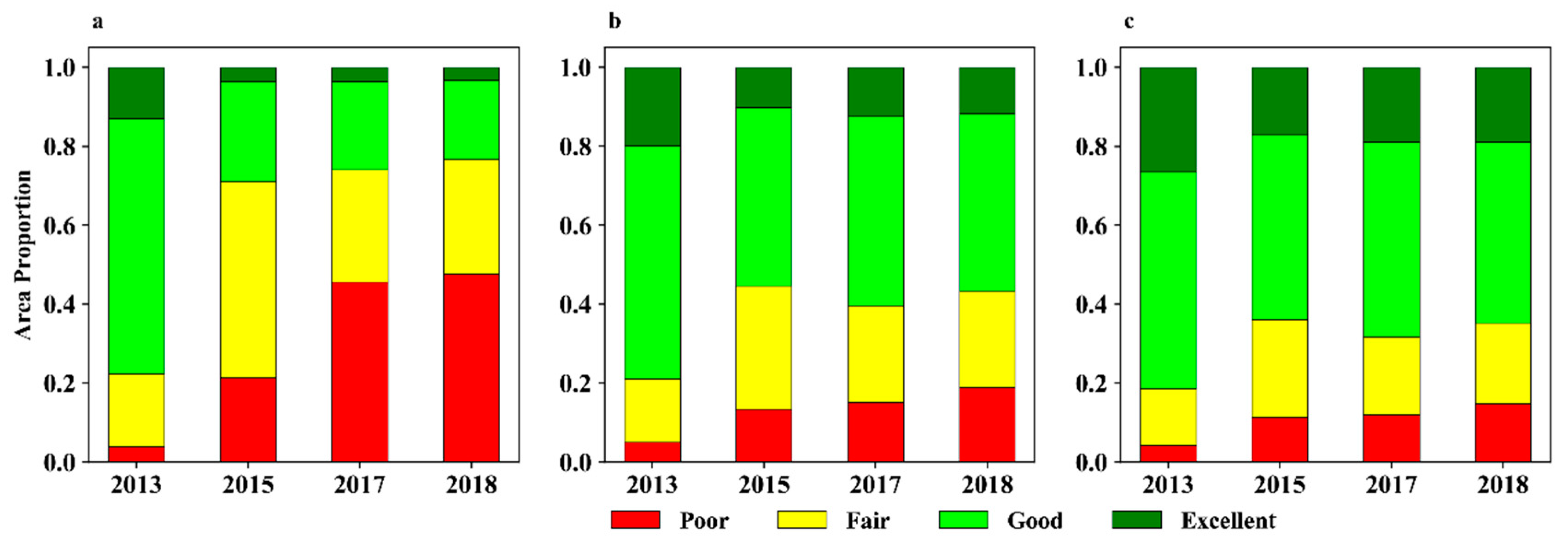
3.3. Changes in Ecological Conditions

The overall spatial and temporal changes in LST in different buffer zones along the highway are shown in Figure 5. The LST experienced the greatest change in the 0–100 m buffer compared with that in the 100–500 m and 500–1000 m buffers. Specifically, the mean and median LST in the 0–100 m buffer increased about 10% per year after highway construction since 2013, reaching the highest level in 2018. Meanwhile, the mean and median LST in the 100–500 m buffer increased by about 5% each year from 2014 whereas that in the 500–1000 m buffer remained relatively stable before and after highway construction. It is noteworthy that the variation of LST, as shown by the inter-quantile range (IQR) of the LST (Figure 5), increased among all buffer zones after highway construction from 2014–2015 and remained high thereafter.
The NDMI in the 0–100 m zone decreased drastically from 2014 to 2015, with the median value decreasing from 0.95 in 2013 to 0.41 in 2015, and it then increased linearly to 0.63 in 2018 (Figure 6). In contrast, the decrease of the NDMI in the 100–500 m zone was relatively smaller, but still obvious, with the median decreasing from 0.98 in 2014 to 0.78 in 2015, and then gradually increasing to 0.87 in 2018. The median and mean NDMI in the 500–1000 m buffer were relatively stable, although they decreased slightly in 2015. The median NDMI in the 500–1000 m zone experienced little change. During the highway construction period, the IQR of the NDMI increased drastically from the early stage of the highway construction in all three buffer zones, followed by a gradual decrease in the IQR from 2015 to 2018.
The NDVI for different years and in three buffer zones is summarized in Figure 7. The median of the NDVI values in the 0–100 m zone decreased quickly from 0.95 in 2013 to 0.63 in 2015; the median NDVI values showed some recovery since 2016 and reached 0.67 in 2018. The median of the NDVI values in the 100–500 m buffer decreased slightly from 0.98 in 2014 to 0.92 in 2015 and to 0.88 in 2016, and then remained relatively stable afterwards. In contrast, the median NDVI values in the 500–1000 m zone changed little from 2013 to 2018. The change in the IQR was very similar across the three buffer zones: it expanded gradually from 2014 to 2016 during highway construction and then gradually shrank.

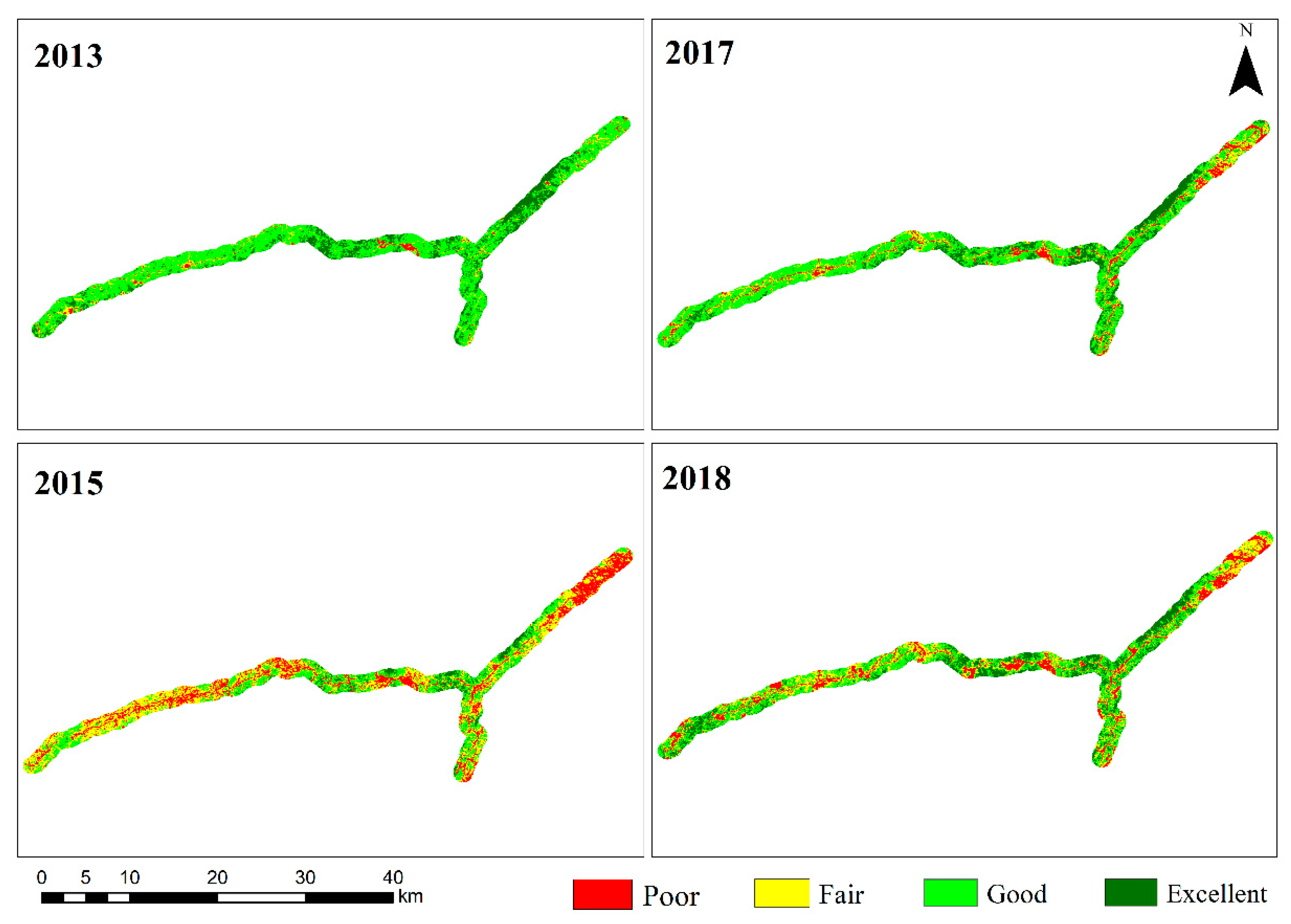
3.4. Overall Change in Ecological Quality Index

Among all three zones, the EQI experienced the most drastic changes in the 0–100 m buffer (Figure 8 and Figure 9). Poor EQI accounted for only less than 5% of the total area in 2013, but it climbed gradually to almost 50% in 2015. Meanwhile, the share for the excellent EQI fell from 12% in 2013 to 2% in 2018; the share for good EQI fell from 75% in 2013 to 17% in 2018; the share for fair EQI increased from 20% in 2013 to 50% in 2015, and then decreased to 26% in 2018. In summary, the overall EQI in the 0–100 m zone fell from predominantly good and excellent (76%) in 2013 to predominantly poor and fair (75%) in 2018.
The area changes of the EQI classes in the 100–500 m zone were different from those in the 0–100 m zone. The trends of the poor and fair classes were similar to those in the 0–100 m zone, although the magnitude of change was smaller. The share for poor EQI increased gradually over time, from 5% in 2013 to 15% in 2018. At the same time, the share for fair EQI first increased from 15% in 2013 to 30% in 2015 and then decreased to 25% in 2018. The decrease in the fractions of the good and excellent classes was smaller as well in comparison to that in the 0–100 m zone. The share for good EQI decreased from 65% in 2013 to 50% in 2015, and showed no obvious change after that. The excellent EQI demonstrated a similar change pattern.
The temporal changes of the four EQI classes in the 500–1000 m buffer zone were similar to those in the 100–500 m zone. However, the change rates of the EQI were relatively smaller, except for the poor class, which increased from 5% to 16%. The total area for the poor and fair EQI classes was 20% in 2013 and increased to 35% in 2018. Correspondingly, the fraction for the good and excellent classes decreased from 80% in 2013 to 65% in 2018.

4. Discussion

4.1. The Effect Distance of Highway

An important question for management and mitigation of road effects on the environment is that of how far from the road its effects extend [11,18]. Among the spatial buffers (0–100 m, 100–500 m, and 500–1000 m) in our analysis, the mean and median value for the NDVI, NDMI, and LST showed substantial changes at a perpendicular distance of <500 m from the highway axis that stabilized at the 500–1000 m zone during the study period. Thus, the road-effect distance determined by the mean and median values was found to be 500 m from highway. This finding is consistent with pervious observations that found effect distances of 400 m for desert tortoises (Gopherus agassizii) [17], 250–1000 m for five species of anurans [18], 1300 m for great bustards (Otis tarda) [19], and 400 m for land-use types [20].
It was unexpected that the road-effect distance determined by spatial variations of these three indicators could extend to 1000 m, and the spatial variations still showed obvious change in the 500–1000 m zone after 2017. This was inconsistent with the result determined by the mean and median values, which showed no significant changes in the 500–1000 m zone. For example, while the median NDVI and NDMI recovered in the 500–1000 m in 2018, the spatial variability of these two indicators showed no sign of recovery. Consequently, the results demonstrated that using the mean and median conditions as the only criteria for quantifying the road-effect distance was inappropriate. The spatial variability, mean, and median values should be considered simultaneously when exploring the effect distance of highway construction.
Our results suggested that the effect distance of the Wujing highway was at least 1000 m from the highway, demonstrated from the spatial and temporal changes of the biophysical indicators and their IQR values. However, due to the recovery and protection policy conducted in the later stage, the road-effect zones for the NDVI, NDMI, and LST will change in the three buffers over time. This is consistent with findings for the Qinghai–Tibet Plateau [14] from a study that examined the impacts of linear infrastructure projects, both highways and railways, on permafrost degradation and vegetation conditions. The authors found that the effect of the engineering activities on vegetation was most evident within a 3000 × 3000 m area, roughly equivalent to 1500 m on each side of the linear infrastructure, and no influence was found beyond 2000 m. Our results were also consistent with the road-effect zones of wildlife activities, which usually extend outward to tens to a few thousands of meters from roads [6].
The mixed effects of highway construction on vegetation, surface moisture, and temperature coexisted and coevolved in a perpendicular distance from the road [18,25,74]. For example, the NDVI and NDMI, as shown in this study, decreased substantially in the 0–100 m and 100–500 m buffers, whereas the LST increased progressively during the study period. A decrease in the NDVI and NDMI could be attributed to the direct removal of vegetation, similar to that of urbanization [75,76], and indirect influences from highway construction, such as changes of moisture and temperature conditions and deposition of dust on vegetation [77,78]. The dust deposited on leaf surfaces could reduce NDVI values by blocking reflectance properties of the underlying leaves in the regions nearest the road [77], therefore reducing photosynthetic activities of vegetation. Nitrogen from vehicular NOX emission could affect vegetation up to 400 m from highway [79,80]. Vegetation deterioration leads to surface exposure and thereby increases the absorption of solar radiation [81], which eventually elevates the land surface temperature. Furthermore, vegetation plays an important role in solar energy transformation by consuming a large proportion of incident solar radiation for water evaporation in the process of evapotranspiration [82]; thus, vegetation removal and a decrease in surface moisture would lead to an increase in surface temperature.
The road-effect zone varied longitudinally and was typically asymmetric with convoluted boundaries, reflecting the coevolution of diverse ecological variables, plus unequal topography and land cover patches on opposite sides of the road, consistent with previous findings [15,83,84]. For example, in the east and west of the WJH, where there is flat terrain and sparse vegetation, the effect distance appeared to extend at least 500 m, whereas in the Chengbu section, where there is mountainous terrain and high forest coverage, the effect distance stabilized in 100–500 m from the highway axis. In terms of the longitudinal changes of the road-effect distance, the environment quality index showed clearly that the most pronounced changes in the EQI were found near Wugang City, where extensive construction disturbance occurred, whilst with the extension of the road to Jingzhou City in the west section, the EQI did not show obvious degradation (Figure 7).

4.2. Environmental Recovery after Highway Construction

Highway construction with detrimental consequences for ecosystems affects the environment and its components [36,85]. In general, highway construction projects dissect the land, leading to habitat fragmentation, shrinkage, and attrition [11], creating effects during construction [85]. In this study, the ecological receptors, such as the NDVI and NDMI, declined around the highway zone. The maximal relative changes in the annual means of the NDVI, NDMI, and LST were about −40%, −60%, and 12%, respectively, in the 0–100 m buffer since 2013. Furthermore, the land cover composition also experienced large changes in the 0–100 m and 100–500 m buffers after the highway construction. This was due to the transition from natural landscapes to impervious surfaces, which led to the initiation or acceleration of destructive processes such as soil erosion [86] and vegetation degradation [87].
Nevertheless, after highway construction finished in 2017, the vegetation and moisture conditions gradually recovered in the later stage: the NDVI and NDMI in the 100 m buffer recovered by about 3% and 12% per year, respectively, probably benefitting from environmental restoration efforts (e.g., slope protection and greening) put in place to prevent soil erosion and vegetation degradation since 2016. Noticeably, the natural forests and artificial mixed forests along the highway were well protected, as indicated by the relatively smaller temporal changes of the EQI along some sections of the road. This effect might be attributable to the government policies geared to improving forest quality and the proportions of natural and mixed forests in the region [88,89]. For example, due to the Sloping Land Conversion From Cropland to Forest program, a program implemented nationally to curb soil erosion and promote ecological restoration [90], vegetation, temperature, and surface wetness can all work together to improve the environment quality.

4.3. Overall Change of EQI

The model used, which consisted of compound indicators including the NDVI, NDMI, LST, and terrain indicators, effectively revealed the integrated impact of highway construction, expressed as the area changes of the four quality classes. From 2013 to 2015, the areas in the fair and poor categories exhibited upward trends while the good and excellent categories decreased rapidly with the road expansion. This corresponded well with land cover conversion and landscape fragmentation due to highway construction and associated urbanization. After completion of the highway at the end of 2017, the fractions of poor and fair quality areas decreased while the good and excellent quality areas began to increase. The fast restoration of EQI following the completion of highway construction can be partially attributed to the environmental restoration efforts, such as the slope protection and greening put in place to prevent soil erosion and vegetation degradation.
This study found that the overall distribution of the EQI changes was uneven across the road zone. The EQI in the 0–100 m and 100–500 m buffer declined faster than that in the 500–1000 m zone, probably caused by the expansion of construction land, cultivated land, and/or unused land. Among these three buffers, the EQI in the 500–1000 m buffer remained relatively stable compared to that in the 0–100 m and 100–500 m zones. However, this does not suggest that there was no impact in the 500–1000 m buffer away from the highway, because the poor grade area in the 500–1000 m zone increased from 2013 to 2018. However, the overall EQI along the road zone began to recover after the highway construction in 2017, resulting from the implementation of environmental restoration projects, such as elimination of illegal logging and deforestation to gain farming fields and grazing [25].

4.4. A Remote Sensing Approach for Monitoring the Ecological Impacts of Infrastructure Projects

The before–during–after control-impact approach had been widely used to guide the collection of field samples for assessing the impacts of human infrastructures on the environment [11,19,51]. The BDACI approach in essence reduces the effects of temporal and spatial variations by subtracting naturally varying temporal effects. This is a key advantage because one of the main challenges in assessing the environmental impacts of engineering works is addressing the large temporal changes of environmental indicators before, during, and after the construction of infrastructures [19,51,91]. However, there are very few published examples of the use of BDACI for assessing the environmental impacts of roads, mainly because of the need for repetitive sampling over time, which is expensive and difficult to achieve [19]. The BDACI-RS approach proposed in this study could overcome the difficulties in applying the traditional BDACI approach and compliment BDACI by adding the remote sensing capability to the overall assessment of the environmental effects of roads. Overall, BDACI-RS could be used practically and in a cost-effective manner to monitor environmental changes during infrastructure construction and operation, which is essential to support decision-making and mitigation activities.
Using the remote sensing images individually, one could monitor the spatial changes of ecological processes resulted from various human activities and natural disturbances [92]. Many multidisciplinary studies had been conducted to evaluate the potential ecological effects of roads. However, quantifying the spatial and temporal changes using infrequent remote sensing images, such as in humid areas with extensive cloud cover, can be challenging [50]. Therefore, instead of using the remote sensing images directly, we first normalized the images using the data from the nearby reference areas to minimize the impacts of spatial and temporal heterogeneity of the acquired images. This normalization process makes all the images comparable in time and space. The BDACI-RS approach is generic and in principal can be applied to assess the impacts of any kind of disturbance and engineering work, such as highway construction.
The approach proposed in this study can quantitatively characterize the road-effect distances of the environmental indicators that can be derived from remotely sensed data. However, the road-effect distances of other essential indicators, including traffic noise pollution, air pollution, and animal movement along the highway, must still rely on field-based observations. Furthermore, the quality of the chosen reference zone can impact the results of the BDACI-RS approach. Therefore, efforts should be put in place to locate the best reference zone representing the undisturbed environment as close as possible to the road being investigated.

5. Conclusions

In this study, we proposed the BDACI-RS approach, and applied it to quantify the spatial and temporal changes of environmental impacts resulting from the construction of the WJH in Hunan province. The main findings are summarized below.
This study developed the BDACI-RS approach to quantify the effect distance of a highway using remotely sensed data; this approach can be readily applied to other regions to map and explore the spatial and temporal changes of disturbances resulting from highway systems. In addition, our study revealed that using the changes in mean and median conditions, as done in many previous studies, cannot effectively determine the road-effect distance. We found that the change of the spatial variability of ecological conditions should be considered simultaneously with the changes in mean and median values when exploring the effect distance of highway construction. The effect distance of the WJH was at least 1000 m from the highway, as demonstrated by the spatial changes of the indicators (both means and spatial variability).
Highway construction greatly affected the land use and land cover in the proximity of highway. Large LULC changes were found in the 0–100 m and 100–500 m buffers, compared with those in the 500–1000 m zone. Vegetation and moisture conditions, indicated by the normalized difference vegetation index and the normalized difference moisture index, respectively, demonstrated obvious decrease–increase (i.e., degradation–recovery) trends in the 0–100 m and 100–500 m buffers, corresponding well with highway construction and operation phases, while land surface temperature showed a progressive increase. An integrated environment quality index, defined by the NDVI, LST, NDMI, and slope, showed that the environmental impact of the highway manifested the most in its close proximity and faded away with distance.

Author Contributions

S.L. designed the research; S.F., S.L. performed research; and S.F., S.L., L.J., Y.Z., W.Y., B.J., M.L., W.L., Y.N., Z.W., Q.L. and J.J. contributed to the writing of the paper. All authors have read and agreed to the published version of the manuscript.

Funding

This research was funded by the National Natural Science Foundation of China, grant numbers: U20A2089 and 41971152 and the Hunan Innovative Talent Program to SL, grant number: 2019RS1062.

Acknowledgments

This work was supported by research grants from the National Natural Science Foundation of China (U20A2089 and 41971152) and Hunan Innovative Talent Program (2019RS1062) to S.L. We thank the anonymous reviewers for their valuable comments.

Conflicts of Interest

The authors declare that they have no known competing financial interests or personal relationships that could have appeared to influence the work reported in this paper.

References

  1. Weiss, D.J.; Nelson, A.; Gibson, H.; Temperley, W.; Peedell, S.; Lieber, A.; Hancher, M.; Poyart, E.; Belchior, S.; Fullman, N. A global map of travel time to cities to assess inequalities in accessibility in 2015. Nature 2018, 553, 333. [Google Scholar] [CrossRef]
  2. Dulac, J. Global Land Transport Infrastructure Requirements; International Energy Agency: Paris, France, 2013; Volume 20, p. 2014. [Google Scholar]
  3. Perz, S.G. Sustainable development: The promise and perils of roads. Nature 2014, 513, 178. [Google Scholar] [CrossRef] [PubMed]
  4. Creutzig, F.; Jochem, P.; Edelenbosch, O.Y.; Mattauch, L.; van Vuuren, D.P.; McCollum, D.; Minx, J. Transport: A roadblock to climate change mitigation? Science 2015, 350, 911–912. [Google Scholar] [CrossRef] [PubMed] [Green Version]
  5. Shannon, G.; Angeloni, L.M.; Wittemyer, G.; Fristrup, K.M.; Crooks, K.R. Road traffic noise modifies behaviour of a keystone species. Anim. Behav. 2014, 94, 135–141. [Google Scholar] [CrossRef]
  6. Torres, A.; Jaeger, J.A.; Alonso, J.C. Assessing large-scale wildlife responses to human infrastructure development. Proc. Natl. Acad. Sci. USA 2016, 113, 8472–8477. [Google Scholar] [CrossRef] [PubMed] [Green Version]
  7. Brady, S.P.; Richardson, J.L. Road ecology: Shifting gears toward evolutionary perspectives. Front. Ecol. Environ. 2017, 15, 91–98. [Google Scholar] [CrossRef]
  8. Meijer, J.R.; Huijbregts, M.A.; Schotten, K.C.; Schipper, A.M. Global patterns of current and future road infrastructure. Environ. Res. Lett. 2018, 13, 064006. [Google Scholar] [CrossRef] [Green Version]
  9. Southworth, J.; Marsik, M.; Qiu, Y.; Perz, S.; Cumming, G.; Stevens, F.; Rocha, K. Roads as drivers of change: Trajectories across the tri-national frontier in MAP, the Southwestern Amazon. Remote Sens. 2011, 3, 1047–1066. [Google Scholar] [CrossRef] [Green Version]
  10. Ibisch, P.L.; Hoffmann, M.T.; Kreft, S.; Pe’er, G.; Kati, V.; Biber-Freudenberger, L.; DellaSala, D.A.; Vale, M.M.; Hobson, P.R.; Selva, N. A global map of roadless areas and their conservation status. Science 2016, 354, 1423–1427. [Google Scholar] [CrossRef]
  11. Forman, R.T.; Alexander, L.E. Roads and their major ecological effects. Annu. Rev. Ecol. Syst. 1998, 29, 207–231. [Google Scholar] [CrossRef] [Green Version]
  12. Klarenberg, G.; Muñoz-Carpena, R.; Campo-Bescós, M.A.; Perz, S.G. Highway paving in the southwestern Amazon alters long-term trends and drivers of regional vegetation dynamics. Heliyon 2018, 4, e00721. [Google Scholar] [CrossRef] [PubMed]
  13. Forman, R.T. Estimate of the area affected ecologically by the road system in the United States. Conserv. Biol. 2000, 14, 31–35. [Google Scholar] [CrossRef]
  14. Song, Y.; Jin, L.; Wang, H. Vegetation changes along the Qinghai-Tibet Plateau engineering corridor since 2000 induced by climate change and human activities. Remote Sens. 2018, 10, 95. [Google Scholar] [CrossRef] [Green Version]
  15. Forman, R.T.; Deblinger, R.D. The ecological road-effect zone of a Massachusetts (USA) suburban highway. Conserv. Biol. 2000, 14, 36–46. [Google Scholar] [CrossRef]
  16. Carr, L.W.; Fahrig, L. Effect of road traffic on two amphibian species of differing vagility. Conserv. Biol. 2001, 15, 1071–1078. [Google Scholar] [CrossRef]
  17. Boarman, W.; Sazaki, M. A highway’s road-effect zone for desert tortoises (Gopherus agassizii). J. Arid Environ. 2006, 65, 94–101. [Google Scholar] [CrossRef]
  18. Eigenbrod, F.; Hecnar, S.J.; Fahrig, L. Quantifying the road-effect zone: Threshold effects of a motorway on anuran populations in Ontario, Canada. Ecol. Soc. 2009, 14, 24. [Google Scholar] [CrossRef] [Green Version]
  19. Torres, A.; Palacín, C.; Seoane, J.; Alonso, J.C. Assessing the effects of a highway on a threatened species using before–during–after and before–during–after-Control–Impact designs. Biol. Conserv. 2011, 144, 2223–2232. [Google Scholar] [CrossRef]
  20. Wu, C.-F.; Lin, Y.-P.; Chiang, L.-C.; Huang, T. Assessing highway’s impacts on landscape patterns and ecosystem services: A case study in Puli Township, Taiwan. Landsc. Urban Plan. 2014, 128, 60–71. [Google Scholar] [CrossRef]
  21. Assis, J.C.; Giacomini, H.C.; Ribeiro, M.C. Road Permeability Index: Evaluating the heterogeneous permeability of roads for wildlife crossing. Ecol. Indic. 2019, 99, 365–374. [Google Scholar] [CrossRef]
  22. Guisande, C.; Rueda-Quecho, A.J.; Rangel-Silva, F.A.; Ríos-Vasquez, J.M. EIA: An algorithm for the statistical evaluation of an environmental impact assessment. Ecol. Indic. 2018, 93, 1081–1088. [Google Scholar] [CrossRef]
  23. Schäfer, R.B.; Bundschuh, M.; Rouch, D.A.; Szöcs, E.; Peter, C.; Pettigrove, V.; Schulz, R.; Nugegoda, D.; Kefford, B.J. Effects of pesticide toxicity, salinity and other environmental variables on selected ecosystem functions in streams and the relevance for ecosystem services. Sci. Total Environ. 2012, 415, 69–78. [Google Scholar] [CrossRef]
  24. Wu, L.; Ye, K.; Gong, P.; Xing, J. Perceptions of governments towards mitigating the environmental impacts of expressway construction projects: A case of China. J. Clean. Prod. 2019, 236, 117704. [Google Scholar] [CrossRef]
  25. Giunta, M. Assessment of the environmental impact of road construction: Modelling and prediction of fine particulate matter emissions. Build. Environ. 2020, 176, 106865. [Google Scholar] [CrossRef]
  26. Jones, J.A.; Swanson, F.J.; Wemple, B.C.; Snyder, K.U. Effects of roads on hydrology, geomorphology, and disturbance patches in stream networks. Conserv. Biol. 2000, 14, 76–85. [Google Scholar] [CrossRef]
  27. Mo, W.; Wang, Y.; Zhang, Y.; Zhuang, D. Impacts of road network expansion on landscape ecological risk in a megacity, China: A case study of Beijing. Sci. Total Environ. 2017, 574, 1000–1011. [Google Scholar] [CrossRef] [PubMed] [Green Version]
  28. Gülci, S.; Akay, A.E.; Oğuz, H.; Gülci, N. Assessment of the road impacts on coniferous species within the road-effect zone using NDVI analysis approach. Fresenius Environ. Bull. 2017, 26, 1654–1662. [Google Scholar]
  29. Alphan, H.; Derse, M.A. Change detection in Southern Turkey using normalized difference vegetation index (NDVI). J. Environ. Eng. Landsc. Manag. 2013, 21, 12–18. [Google Scholar] [CrossRef]
  30. Vollmer, D.; Shaad, K.; Souter, N.J.; Farrell, T.; Dudgeon, D.; Sullivan, C.A.; Fauconnier, I.; Macdonald, G.M.; Mccartney, M.P.; Power, A.G.; et al. Integrating the social, hydrological and ecological dimensions of freshwater health: The Freshwater Health Index. Sci. Total Environ. 2018, 627, 304–313. [Google Scholar] [CrossRef] [PubMed]
  31. Messager, M.L.; Lehner, B.; Grill, G.; Nedeva, I.; Schmitt, O. Estimating the volume and age of water stored in global lakes using a geo-statistical approach. Nat. Commun. 2016, 7, 13603. [Google Scholar] [CrossRef] [PubMed]
  32. Chi, Y.; Zhang, Z.; Gao, J.; Xie, Z.; Zhao, M.; Wang, E. Evaluating landscape ecological sensitivity of an estuarine island based on landscape pattern across temporal and spatial scales. Ecol. Indic. 2019, 101, 221–237. [Google Scholar] [CrossRef]
  33. Clements, G.R. The environmental and social impacts of roads in Southeast Asia. Ph.D. Thesis, James Cook University, Townsville, Australia, 2013. [Google Scholar]
  34. Pettorelli, N.; Vik, J.O.; Mysterud, A.; Gaillard, J.-M.; Tucker, C.J.; Stenseth, N.C. Using the Satellite-Derived NDVI to Sssess Ecological Responses to Environmental Change. Trends Ecol. Evol. 2005, 20, 503–510. [Google Scholar] [CrossRef] [PubMed]
  35. Gao, B.-C. NDWI—A normalized difference water index for remote sensing of vegetation liquid water from space. Remote Sens. Environ. 1996, 58, 257–266. [Google Scholar] [CrossRef]
  36. Nedbal, V.; Brom, J. Impact of highway construction on land surface energy balance and local climate derived from LANDSAT satellite data. Sci. Total Environ. 2018, 633, 658–667. [Google Scholar] [CrossRef]
  37. Liu, M.; Yang, W.; Zhu, X.; Chen, J.; Chen, X.; Yang, L.; Helmer, E.H. An Improved Flexible Spatiotemporal DAta Fusion (IFSDAF) method for producing high spatiotemporal resolution normalized difference vegetation index time series. Remote Sens. Environ. 2019, 227, 74–89. [Google Scholar] [CrossRef]
  38. Carlson, T.N.; Ripley, D.A. On the relation between NDVI, fractional vegetation cover, and leaf area index. Remote Sens. Environ. 1997, 62, 241–252. [Google Scholar] [CrossRef]
  39. Zhang, J.; Zhang, L.; Xu, C.; Liu, W.; Qi, Y.; Wo, X. Vegetation variation of mid-subtropical forest based on MODIS NDVI data—A case study of Jinggangshan City, Jiangxi Province. Acta Ecol. Sin. 2014, 34, 7–12. [Google Scholar] [CrossRef]
  40. Karan, S.K.; Samadder, S.R.; Maiti, S.K. Assessment of the capability of remote sensing and GIS techniques for monitoring reclamation success in coal mine degraded lands. J. Environ. Manag. 2016, 182, 272–283. [Google Scholar] [CrossRef] [PubMed]
  41. Hardisky, M.; Klemas, V.; Smart, M. The influence of soil salinity, growth form, and leaf moisture on the spectral radiance of. Spartina Alterniflora 1983, 49, 77–83. [Google Scholar]
  42. Zhang, H.; Gorelick, S.M.; Zimba, P.V.; Zhang, X. A remote sensing method for estimating regional reservoir area and evaporative loss. J. Hydrol. 2017, 555, 213–227. [Google Scholar] [CrossRef]
  43. Rozenstein, O.; Qin, Z.; Derimian, Y.; Karnieli, A. Derivation of land surface temperature for Landsat-8 TIRS using a split window algorithm. Sensors 2014, 14, 5768–5780. [Google Scholar] [CrossRef]
  44. Owen, T.; Carlson, T.; Gillies, R. An assessment of satellite remotely-sensed land cover parameters in quantitatively describing the climatic effect of urbanization. Int. J. Remote Sens. 1998, 19, 1663–1681. [Google Scholar] [CrossRef]
  45. Chen, X.-L.; Zhao, H.-M.; Li, P.-X.; Yin, Z.-Y. Remote sensing image-based analysis of the relationship between urban heat island and land use/cover changes. Remote Sens. Environ. 2006, 104, 133–146. [Google Scholar] [CrossRef]
  46. Li, W.; Cao, Q.; Lang, K.; Wu, J. Linking potential heat source and sink to urban heat island: Heterogeneous effects of landscape pattern on land surface temperature. Sci. Total Environ. 2017, 586, 457–465. [Google Scholar] [CrossRef] [PubMed]
  47. Wang, Y.-C.; Hu, B.K.; Myint, S.W.; Feng, C.-C.; Chow, W.T.; Passy, P.F. Patterns of land change and their potential impacts on land surface temperature change in Yangon, Myanmar. Sci. Total Environ. 2018, 643, 738–750. [Google Scholar] [CrossRef]
  48. Simwanda, M.; Ranagalage, M.; Estoque, R.C.; Murayama, Y. Spatial analysis of surface urban heat islands in four rapidly growing African Cities. Remote Sens. 2019, 11, 1645. [Google Scholar] [CrossRef] [Green Version]
  49. Fluet-Chouinard, E.; Lehner, B.; Rebelo, L.-M.; Papa, F.; Hamilton, S.K. Development of a global inundation map at high spatial resolution from topographic downscaling of coarse-scale remote sensing data. Remote Sens. Environ. 2015, 158, 348–361. [Google Scholar] [CrossRef]
  50. Feng, S.; Liu, S.; Huang, Z.; Jing, L.; Zhao, M.; Peng, X.; Yan, W.; Wu, Y.; Lv, Y.; Smith, A.R. Inland water bodies in China: Features discovered in the long-term satellite data. Proc. Natl. Acad. Sci. USA 2019, 116, 25491–25496. [Google Scholar] [CrossRef] [Green Version]
  51. Roedenbeck, I.A.; Fahrig, L.; Findlay, C.S.; Houlahan, J.E.; Jaeger, J.A.; Klar, N.; Kramer-Schadt, S.; van der Grift, E.A. The Rauischholzhausen agenda for road ecology. Ecol. Soc. 2007, 12, 11. [Google Scholar] [CrossRef]
  52. Abo-Qudais, S.; Alhiary, A. Effect of distance from road intersection on developed traffic noise levels. Can. J. Civ. Eng. 2004, 31, 533–538. [Google Scholar] [CrossRef]
  53. Raaschou-Nielsen, O.; Andersen, Z.J.; Hvidberg, M.; Jensen, S.S.; Ketzel, M.; Sørensen, M.; Hansen, J.; Loft, S.; Overvad, K.; Tjønneland, A. Air pollution from traffic and cancer incidence: A Danish cohort study. Environ. Health 2011, 10, 67. [Google Scholar] [CrossRef] [Green Version]
  54. Chen, L.-C.; Kendall, M.; Thurston, G.D. Personal Exposures to Traffic-Related Air Pollution and Acute Respiratory Health among Bronx School Children. Environ. Health Perspect. 2011, 119, 559. [Google Scholar]
  55. Raymond, P.A.; Hartmann, J.; Lauerwald, R.; Sobek, S.; C McDonald, M.; Hoover, D.; Butman, R.; Striegl, E.M.; Humborg, C. Global carbon dioxide emissions from inland waters. Nature 2013, 503, 355. [Google Scholar] [CrossRef] [PubMed] [Green Version]
  56. Deng, C.; Wu, C. Examining the impacts of urban biophysical compositions on surface urban heat island: A spectral unmixing and thermal mixing approach. Remote Sens. Environ. 2013, 131, 262–274. [Google Scholar] [CrossRef]
  57. Liu, W.; Zhan, J.; Zhao, F.; Yan, H.; Zhang, F.; Wei, X. Impacts of urbanization-induced land-use changes on ecosystem services: A case study of the Pearl River Delta Metropolitan Region, China. Ecol. Indic. 2019, 98, 228–238. [Google Scholar] [CrossRef]
  58. Li, H.; Peng, J.; Liu, Y.; Hu, Y. Urbanization impact on landscape patterns in Beijing City, China: A spatial heterogeneity perspective. Ecol. Indic. 2017, 82, 50–60. [Google Scholar] [CrossRef]
  59. Raiter, K.G.; Prober, S.M.; Possingham, H.P.; Westcott, F.; Hobbs, R.J. Linear infrastructure impacts on landscape hydrology. J. Environ. Manag. 2018, 206, 446–457. [Google Scholar] [CrossRef]
  60. Fei, W.; Zhao, S. Urban land expansion in China’s six megacities from 1978 to 2015. Sci. Total Environ. 2019, 664, 60–71. [Google Scholar] [CrossRef] [PubMed]
  61. Zhao, H.; Cui, B.; Zhang, H.; Fan, X.; Zhang, Z.; Lei, X. A landscape approach for wetland change detection (1979–2009) in the Pearl River Estuary. Procedia Environ. Sci. 2010, 2, 1265–1278. [Google Scholar] [CrossRef] [Green Version]
  62. Xu, C.; Zhao, S.; Liu, S. Spatial scaling of multiple landscape features in the conterminous United States. Landsc. Ecol. 2019, 35, 223–247. [Google Scholar] [CrossRef]
  63. McGarigal, K. FRAGSTATS Help; University of Massachusetts: Amherst, MA, USA, 2015. [Google Scholar]
  64. Ramezani, H.; Holm, S.; Allard, A.; Ståhl, G. Monitoring landscape metrics by point sampling: Accuracy in estimating Shannon’s diversity and edge density. Environ. Monit. Assess. 2010, 164, 403–421. [Google Scholar] [CrossRef] [PubMed]
  65. Herold, M.; Scepan, J.; Clarke, K.C. The use of remote sensing and landscape metrics to describe structures and changes in urban land uses. Environ. Plan. A 2002, 34, 1443–1458. [Google Scholar] [CrossRef] [Green Version]
  66. Chen, F.; Chen, J.; Wu, H.; Hou, D.; Zhang, W.; Zhang, J.; Zhou, X.; Chen, L. A landscape shape index-based sampling approach for land cover accuracy assessment. Sci. China Earth Sci. 2016, 59, 2263–2274. [Google Scholar] [CrossRef]
  67. Liu, Y.; Peng, J.; Wang, Y. Efficiency of landscape metrics characterizing urban land surface temperature. Landsc. Urban Plan. 2018, 180, 36–53. [Google Scholar] [CrossRef]
  68. He, H.S.; DeZonia, B.E.; Mladenoff, D.J. J. An aggregation index (AI) to quantify spatial patterns of landscapes. Landsc. Ecol. 2000, 15, 591–601. [Google Scholar]
  69. Hou, H.; Wang, R.; Murayama, Y. Scenario-based modelling for urban sustainability focusing on changes in cropland under rapid urbanization: A case study of Hangzhou from 1990 to 2035. Sci. Total Environ. 2019, 661, 422–431. [Google Scholar] [CrossRef]
  70. Karlson, M.; Mörtberg, U.; Balfors, B. Road ecology in environmental impact assessment. Environ. Impact Assess. Rev. 2014, 48, 10–19. [Google Scholar] [CrossRef]
  71. El-Gafy, M.; Abdelrazig, Y.; Abdelhamid, T. Environmental impact assessment for transportation projects: Case study using remote-sensing technology, geographic information systems, and spatial modeling. J. Urban Plan. Dev. 2011, 137, 153–158. [Google Scholar] [CrossRef]
  72. Ying, X.; Zeng, G.M.; Chen, G.Q.; Tang, L.; Wang, K.L.; Huang, D.Y. Combining AHP with GIS in synthetic evaluation of eco-environment quality—A case study of Hunan Province, China. Ecol. Model. 2007, 209, 97–109. [Google Scholar] [CrossRef]
  73. Foody, G.M. Explaining the unsuitability of the kappa coefficient in the assessment and comparison of the accuracy of thematic maps obtained by image classification. Remote Sens. Environ. 2020, 239, 111630. [Google Scholar] [CrossRef]
  74. Zhou, T.; Luo, X.; Hou, Y.; Xiang, Y.; Peng, S. Quantifying the effects of road width on roadside vegetation and soil conditions in forests. Landsc. Ecol. 2020, 35, 69–81. [Google Scholar] [CrossRef] [Green Version]
  75. Zhao, S.; Liu, S.; Zhou, D. Prevalent vegetation growth enhancement in urban environment. Proc. Natl. Acad. Sci. USA 2016, 113, 6313–6318. [Google Scholar] [CrossRef] [PubMed] [Green Version]
  76. Jia, W.; Zhao, S.; Liu, S. Vegetation growth enhancement in urban environments of the Conterminous United States. Glob. Chang. Biol. 2018, 24, 4084–4094. [Google Scholar] [CrossRef] [PubMed]
  77. Ackerman, D.E.; Finlay, J.C. Road dust biases NDVI and alters edaphic properties in Alaskan arctic tundra. Sci. Rep. 2019, 9, 1–8. [Google Scholar] [CrossRef] [PubMed]
  78. Rahul, J.; Jain, M.K. An investigation in to the impact of particulate matter on vegetation along the national highway: A review. Res. J. Environ. Sci. 2014, 8, 356–372. [Google Scholar] [CrossRef] [Green Version]
  79. Angold, G. The impact of a road upon adjacent heathland vegetation: Effects on plant species composition. J. Appl. Ecol. 1997, 34, 409–417. [Google Scholar] [CrossRef]
  80. Redling, K.; Elliott, E.; Bain, D.; Sherwell, J. Highway contributions to reactive nitrogen deposition: Tracing the fate of vehicular NOx using stable isotopes and plant biomonitors. Biogeochemistry 2013, 116, 261–274. [Google Scholar] [CrossRef]
  81. Li, D.; Liao, W.; Rigden, A.J.; Liu, X.; Wang, D.; Malyshev, S.; Shevliakova, E. Urban heat island: Aerodynamics or imperviousness? Sci. Adv. 2019, 5, eaau4299. [Google Scholar] [CrossRef] [PubMed] [Green Version]
  82. Kunert, N.; Aparecido LM, T.; Higuchi, N.; dos Santos, J.; Trumbore, S. Higher tree transpiration due to road-associated edge effects in a tropical moist lowland forest. Agric. For. Meteorol. 2015, 213, 183–192. [Google Scholar] [CrossRef]
  83. Pariente, S.; Helena, Z.; Eyal, S.; Anatoly, F.G.; Michal, Z. Road side effect on lead content in sandy soil. Catena 2019, 174, 301–307. [Google Scholar] [CrossRef]
  84. Liang, J.; Liu, Y.; Ying, L.; Li, P.; Xu, Y.; Shen, Z. Road impacts on spatial patterns of land use and landscape fragmentation in three parallel rivers region, Yunnan Province, China. Chin. Geogr. Sci. 2014, 24, 15–27. [Google Scholar] [CrossRef] [Green Version]
  85. Spellerberg, I. Ecological effects of roads and traffic: A literature review. Glob. Ecol. Biogeogr. Lett. 1998, 7, 317–333. [Google Scholar] [CrossRef]
  86. Kleinschroth, F.; Laporte, N.; Laurance, W.F.; Goetz, S.J.; Ghazoul, J. Road expansion and persistence in forests of the Congo Basin. Nat. Sustain. 2019, 2, 628–634. [Google Scholar] [CrossRef]
  87. Deljouei, A.; Sadeghi SM, M.; Abdi, E.; Bernhardt-Römermann, M.; Pascoe, E.L.; Marcantonio, M. The impact of road disturbance on vegetation and soil properties in a beech stand, Hyrcanian forest. Eur. J. Res. 2018, 137, 759–770. [Google Scholar] [CrossRef]
  88. Wang, J.; Wang, K.; Zhang, M.; Zhang, C. Impacts of climate change and human activities on vegetation cover in hilly southern China. Ecol. Eng. 2015, 81, 451–461. [Google Scholar] [CrossRef]
  89. Igondova, E.; Pavlickova, K.; Majzlan, O. The ecological impact assessment of a proposed road development (the Slovak approach). Environ. Impact Assess. Rev. 2016, 59, 43–54. [Google Scholar] [CrossRef]
  90. Yuan, W.; Li, X.; Liang, S.; Cui, X.; Dong, W.; Liu, S.; Xia, J.; Chen, Y.; Liu, D.; Zhu, W. Characterization of locations and extents of afforestation from the Grain for Green Project in China. Remote Sens. Lett. 2014, 5, 221–229. [Google Scholar] [CrossRef]
  91. Hu, X.; Xu, H. A new remote sensing index for assessing the spatial heterogeneity in urban ecological quality: A case from Fuzhou City, China. Ecol. Indic. 2018, 89, 11–21. [Google Scholar] [CrossRef]
  92. Reymondin, L.; Argote, K.; Jarvis, A.; Navarrete, C.; Coca, A.; Grossman, D.; Villalba, A.; Suding, P. Road Impact Assessment Using Remote Sensing Methodology for Monitoring Land-Use Change in Latin America: Results of Five Case Studies; Inter-American Development Bank: Washington, DC, USA, 2013. [Google Scholar]
Figure 1. The location of the study area and the Wujing Highway (WJH).
Remotesensing 13 01340 g001
Figure 2. The highway (red line), the buffer zones, and the reference area. (a) The land-use type along the highway derived from the remote sensing data; (b) the reference area is shown by the outer strip with a width of 500 m located 5000 m away from the highway; (c) the three buffers divided along the highway zone.
Remotesensing 13 01340 g002
Figure 3. The land cover and land use change of the WJH from 2013 to 2018.
Remotesensing 13 01340 g003
Figure 4. Land cover compositions in the 0–100 m (a), 100–500 m (b), and 500–1000 m (c) zones perpendicular along the highway.
Remotesensing 13 01340 g004
Figure 5. Temporal changes in the normalized land surface temperature (LST) in different buffer zones along the highway from 2013 to 2018. The top and bottom of the boxes represent 75 and 25 percentiles (i.e., Q3 and Q1), respectively; the line in the box is the median; the height of the whole box is the interquartile range (IQR = Q3 − Q1); the top and bottom whiskers represent the Q3 + 1.5 * IQR and Q1 − 1.5 * IQR values, respectively. This convention is used for other boxplots throughout the paper. P1 and P3 represent the periods before and after highway construction, respectively. P2 represents the period during highway construction.
Remotesensing 13 01340 g005
Figure 6. Temporal changes in the normalized difference moisture index (NDMI) in different zones along the highway from 2013 to 2018. P1 and P3 represent the periods before and after highway construction, respectively. P2 represents the period during highway construction.
Remotesensing 13 01340 g006
Figure 7. Temporal changes in the normalized difference vegetation index (NDVI) in different zones along the highway from 2013 to 2018. P1 and P3 represent the periods before and after highway construction, respectively. P2 represents the period during highway construction.
Remotesensing 13 01340 g007
Figure 8. The ecological impact assessment for the environment quality index (EQI) from 2013 to 2018.
Remotesensing 13 01340 g008
Figure 9. Overall EQI change from 2013 to 2018 in the (a) 100 m buffer, (b)100–500 m buffer, and (c) 500–1000 m buffer.
Remotesensing 13 01340 g009
Table 1. The Landsat data information used in this study.
Landsat Scene IDPathRowData
LC81250422013194LGN001254213 July 2013
LC81250422014165LGN001254214 June 2014
LC81250422015104LGN001254214 April 2015
LC81250422016107LGN001254216 April 2016
LC81250422017125LGN00125425 May 2017
LC81250422018144LGN001254224 May 2018
Table 2. The landscape metrics used in this study.
Landscape MetricsAcronymRangeUnitDescription
Percentage of landscapePLAND0 < PLAND ≤ 100%The percentage the landscape of the corresponding patch type.
Patch densityPDPD > 0number/100 haThe number of patches per 100 hectares.
Edge densityEDED ≥ 0m/haThe length of edge relative to the area of the patch of a land cover type.
Landscape shape indexLSILSI > 0/A perimeter-to-area ratio for the landscape as a whole, indicating the shape complexity of the landscape.
Aggregation IndexAI0 < AI ≤ 100%Degree of aggregation of landscape patch aggregation.
Table 3. The factors of environmental quality evaluation and their weights.
FactorEcological IndicatorWeight
VegetationNDVI0.3
MoistureNDMI0.3
Surface temperatureLST0.2
TopographySlope0.1
ElevationDEM0.1
Table 4. The dynamics of the landscape index during 2013–2018.
YearLULCLandscape Index
PLANDPDEDLSIAI
2013Built-up4.715.2225.4838.8161.15
Water0.760.181.806.7984.98
Cropland18.056.7060.7748.0075.51
Forest76.481.5752.6623.3794.36
2015Built-up11.004.5743.2843.0571.89
Water1.000.041.705.6789.47
Cropland15.7211.0164.2354.2370.27
Forest72.292.7061.4227.3293.17
2017Built-up11.058.2155.7755.1762.18
Water1.040.071.876.1288.14
Cropland13.897.7349.3944.6772.84
Forest74.011.8646.0721.5294.49
2018Built-up13.749.1964.0656.7266.66
Water0.960.071.775.9788.53
Cropland15.3511.2962.2153.0070.59
Forest69.952.1858.8926.8493.19
Publisher’s Note: MDPI stays neutral with regard to jurisdictional claims in published maps and institutional affiliations.

