Article

Mapping the Distribution of Coffee Plantations from Multi-Resolution, Multi-Temporal, and Multi-Sensor Data Using a Random Forest Algorithm

by
Anggun Tridawati
1,2,3,
Ketut Wikantika
1,2,*,
Tri Muji Susantoro
4,
Agung Budi Harto
1,2,
Soni Darmawan
5,
Lissa Fajri Yayusman
2 and
Mochamad Firman Ghazali
3
1
Remote Sensing and Geographic Information Science Research Group, Department of Geodesy and Geomatics, Faculty of Earth Sciences and Technology, Institut Teknologi Bandung, Bandung 40132, Indonesia
2
Center for Remote Sensing, Institut Teknologi Bandung, Bandung 40132, Indonesia
3
Department of Geodesy and Geomatics Engineering, Faculty of Engineering, Universitas Lampung, Sumantri Brojonegoro No 1, Bandar Lampung 35141, Indonesia
4
Research and Development Center for Oil and Gas Technology “LEMIGAS”, Ministry of Energy and Mineral Resources, Jakarta 12230, Indonesia
5
Institut Teknologi Nasional Bandung, PHH Mustofa No 23, Bandung 40124, Indonesia
*
Author to whom correspondence should be addressed.
Remote Sens. 2020, 12(23), 3933; https://doi.org/10.3390/rs12233933
Submission received: 7 October 2020 / Revised: 26 November 2020 / Accepted: 27 November 2020 / Published: 1 December 2020

Abstract

:
Indonesia is the world’s fourth largest coffee producer. Coffee plantations cover 1.2 million ha of the country with a production of 500 kg/ha. However, information regarding the distribution of coffee plantations in Indonesia is limited. This study aimed to assess the accuracy of classification model and determine its important variables for mapping coffee plantations. The model obtained 29 variables which derived from the integration of multi-resolution, multi-temporal, and multi-sensor remote sensing data, namely, pan-sharpened GeoEye-1, multi-temporal Sentinel 2, and DEMNAS. Applying a random forest algorithm (tree = 1000, mtry = all variables, minimum node size: 6), this model achieved overall accuracy, kappa statistics, producer accuracy, and user accuracy of 79.333%, 0.774, 92.000%, and 90.790%, respectively. In addition, 12 most important variables achieved overall accuracy, kappa statistics, producer accuracy, and user accuracy 79.333%, 0.774, 91.333%, and 84.570%, respectively. Our results indicate that random forest algorithm is efficient in mapping coffee plantations in an agroforestry system.

Graphical Abstract

1. Introduction

Coffee is one of the most important trade commodities in the world. Coffee trees were first found in the mountains of Ethiopia in the 9th century. They were planted in Indonesia in 1699 by the Dutch Vereenigde Oostindische Compagnie (VOC). The planting patterns that have been developed by coffee farmers can generally be classified into two categories: monoculture (mono-cropping) and agroforestry [1]. In Indonesia, coffee-based agroforestry is a well-developed model proficient in supporting social, ecological, and economic interests. According to the International Coffee Organization [2], Indonesia is the fourth largest coffee producer in the world, even though Indonesia stands out as having the second-largest amount of land devoted to coffee plantations, after Brazil [3]. Nevertheless, coffee production in Indonesia is relatively low: 500 kg/ha, with a total area of 1.2 million ha. This is in strong contrast to Vietnam which produces 2.7 million tons of coffee per ha, while having a total area of 630,000 ha [4]. Indonesia has a great potential for becoming the largest coffee producer in the world if the country were able to increase its production efficiency. This is supported by high market demand and the availability of land that is highly suited for coffee development. Therefore, the mapping of coffee plantations is essential for identifying the centers of coffee production. Remote sensing technology has been widely proven to be a cost-effective, fast, efficient method that is essential in monitoring and mapping vegetation [5,6].
Several techniques for mapping coffee plantations were previously used by researchers. These include: supervised pixel-based classification [7,8], object-based classification [9,10], hybrid classification [11], use of spectral variables [12], topographic variables [7,13,14], tasseled cap, and the correlation of NDVI and precipitation [14]. Generally, the aforementioned research uses the classification technique. Classification algorithms can be divided into two models: parametric and nonparametric [15]. A parametric algorithm requires statistical parameters derived from normally distributed training data; whereas, a nonparametric algorithm does not require statistical parameters. Most researchers have been using remote sensing data to map coffee plantations to improve accuracy; in general, they have used Maximum Likelihood (ML) as a parametric algorithm [7,12]. The ML algorithm groups pixels based on the probability of a class in normal distribution [16]. However, the normal distribution assumption is often ignored, especially in complex areas (high spectral heterogeneity). This parametric algorithm is also hindered by difficulties in integrating spectral variables with other variables [17].
In the classification process, nonparametric algorithms performed well [17]. The random forest algorithm is one of the most popular nonparametric algorithms and provides high accuracy results [18,19,20,21]. This algorithm is also used to rank variables [22]. Several recent studies have explored the application of random forest algorithms in mapping land cover [20,21,23], invasive plant species [24], landslide areas [25], bamboo patches [26] and larch trees [27]. Kelley et al. [14] used a random forest algorithm from integrating multi-temporal tasseled cap derived from Landsat 8 imagery, temperatures, topography, and precipitation to map coffee plantations in northern Nicaragua which resulted in user accuracy of 82.1% and producer accuracy of 80.0%. Previous studies indicate that the mapping of coffee plantations has mostly been done with medium resolution imagery [11,14]. However, very high-resolution (VHR) satellite imagery is needed for mapping coffee plantations due to 70% of the world’s coffee is grown on small-holder plantations which are less than 10 ha [28].
Since 1999, the availability of VHR imagery such as IKONOS 2, Quickbird, OrbView-3, Rapid-Eye, WorldView-2, and Geo-Eye 1 has made vegetation mapping easier. Pan-sharpened GeoEye-1 is a VHR image that was launched in 2008 with a panchromatic geometric resolution (PAN) of 0.46 m. Aguliar et al. [29] state that pan-sharpened GeoEye-1 achieved higher accuracy than the pan-sharpened WorldView 2 for discriminating shadows, buildings, vacant land, and vegetation. On the other hand, research related to the use of texture in improving the accuracy of mapping coffee plantations has rarely been done. Whereas, it has been found that a combination of spectral images and texture produces a higher accuracy than classifications based only on the spectral image [30]. Other research results indicate that classification accuracy achieved by adding texture variables extracted from ALOS PRISM was higher than when only using a combination of ALOS AVNIR and ASTER GDEM topographical data for the delineation of a Shifting Cultivation Landscape [31]. Gao et al. [27] explain that adding textural variables extracted from Landsat imagery using the random forest algorithm produced an increase in the overall accuracy of 2.92%. Therefore, this research carried out an analysis with the addition of textural variables for mapping coffee plantations in an agroforestry system. It is hoped that the addition of these variables can improve the classification accuracy of coffee plantations.
Coffee trees exhibit different characteristics in different seasons. In rainy season, these trees thrive and have dense green leaves, while in dry season (the harvest period) leaves are reduced due to pruning by coffee farmers. Pruning needs to be done to maintain productivity as well as the sustainability of coffee plantation cultivation. However, this does cause a difference in the spectral value of coffee plantations. Loss of leaves due to pruning results in lower NIR channel values and higher red channel values [32]. Therefore, the use of multi-temporal data becomes an alternative solution to represent the condition of coffee plantations in different seasons through the vegetation index. Multi-temporal data were also very significant for monitoring changes in land cover and plant phenology [33].
Multi-temporal VHR satellite imagery could not be obtained in this research; therefore medium resolution data obtained from Sentinel 2, was used. Jia et al. [33] explain that the addition of multi-temporal data derived from medium-resolution images achieved a significant increase in the accuracy of high-resolution image classification, especially in terms of differentiating plantation types. Souza et al. [10] mapped coffee plantations by integrating multi-temporal variables extracted from Landsat (30 m) and Rapid-Eye imagery (5 m), achieving significant accuracy compared to when only using Rapid-Eye. Sentinel 2 is a new generation of medium-resolution imagery launched in 2015 and has significant potential for mapping coffee plantations [34]. It has 13 bands that consist of the spatial resolution of 10 m (for the visible and near-infrared light bands) and 20 m (for the near-infrared and shortwave infrared bands) from blue wavelengths (0.458–0.523 µm) to SWIR (2.100–2.280 µm) which are sufficient for calculating a range of indices to successfully map coffee plantations. In this research, multi-temporal Sentinel 2 was used as a variable on Landsat 8 for mapping coffee plantations, applying what was used by Kelley et al. [14]. These variables include the multi-temporal vegetation index of greenness, wetness, brightness, slope, aspect, elevation, and multi-temporal NDVI. The main development of this research is the use of VHR satellite imagery obtained from GeoEye-1 and the addition of textural variables; namely, entropy, standard deviation, correlation, mean, and contrast in mapping coffee plantations in the agroforestry system. Therefore, we pursue two primary objectives:
(1)
Assessing the accuracy of random forest classification derived from integrating multi-sensor, multi-temporal, and multi-resolution remote sensing data from pan-sharpened GeoEye-1, multi-temporal Sentinel 2, and DEM for mapping coffee plantations.
(2)
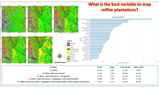
Determining the most important variables derived from random forest classifications for mapping coffee plantations.

2. Materials and Methods

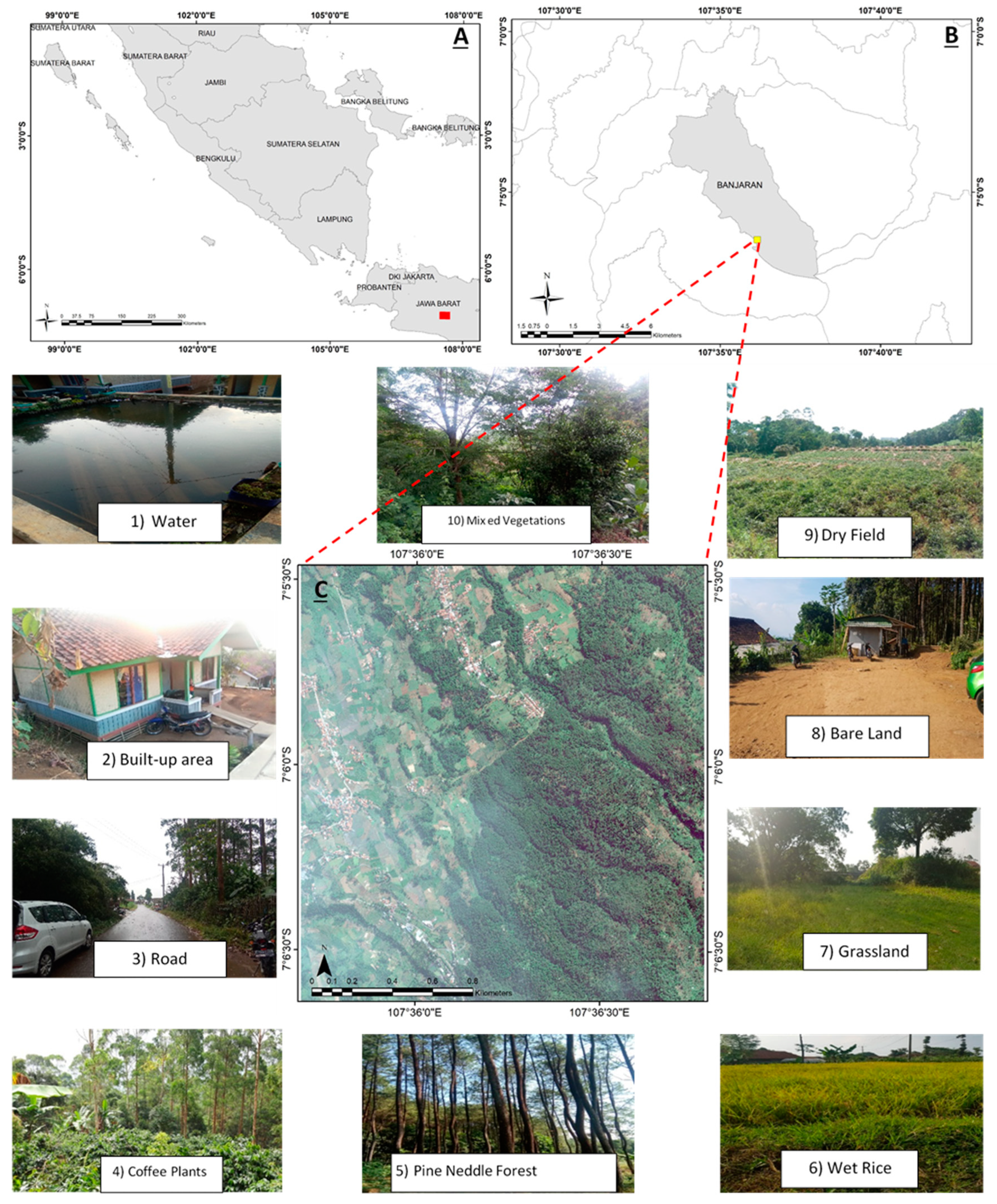
2.1. Description of Research Area

The research was conducted in parts of Mount (Mt.) Puntang, in Banjaran district in West Java, Indonesia. The research area focused on approximately 433.7 ha where is located between 107. 595°E to 107.613°E and 7.091°S to 7.111°S. The area is mainly mountainous from the central portion to the southeast, while the northwestern part is predominantly plain. The elevation ranges between 1000 and 1200 m above sea level, and the terrain is flat to undulating. The annual precipitation is 2500 mm per year.
Coffee plantations have a biannual growing cycle [35]. There are some phases of growing coffee plantations including firstly, the phase correlates to vegetation production from September to March, the second phase is maturation and dormancy of the buds from April to August of the first year, the third phase is flowering of the buds from September to December, the fifth phase is the fruit ripens for three months, and the final phase occurs in July and August of the second year which is the senescence. On the dry season which is the leaves of coffee trees are reduced due to pruning by coffee farmers occurs from March to September, meanwhile on the rainy season which is trees thrive and have dense green leaves occurs from September to March. The research area was chosen due to Mt. Puntang being one of the best coffee production centers in West Java and won an award at the 2016 Specialty Coffee Association of America (SCAA) Contest in Atlanta. The research area can be seen in Figure 1.

2.2. Data and Preprocessing
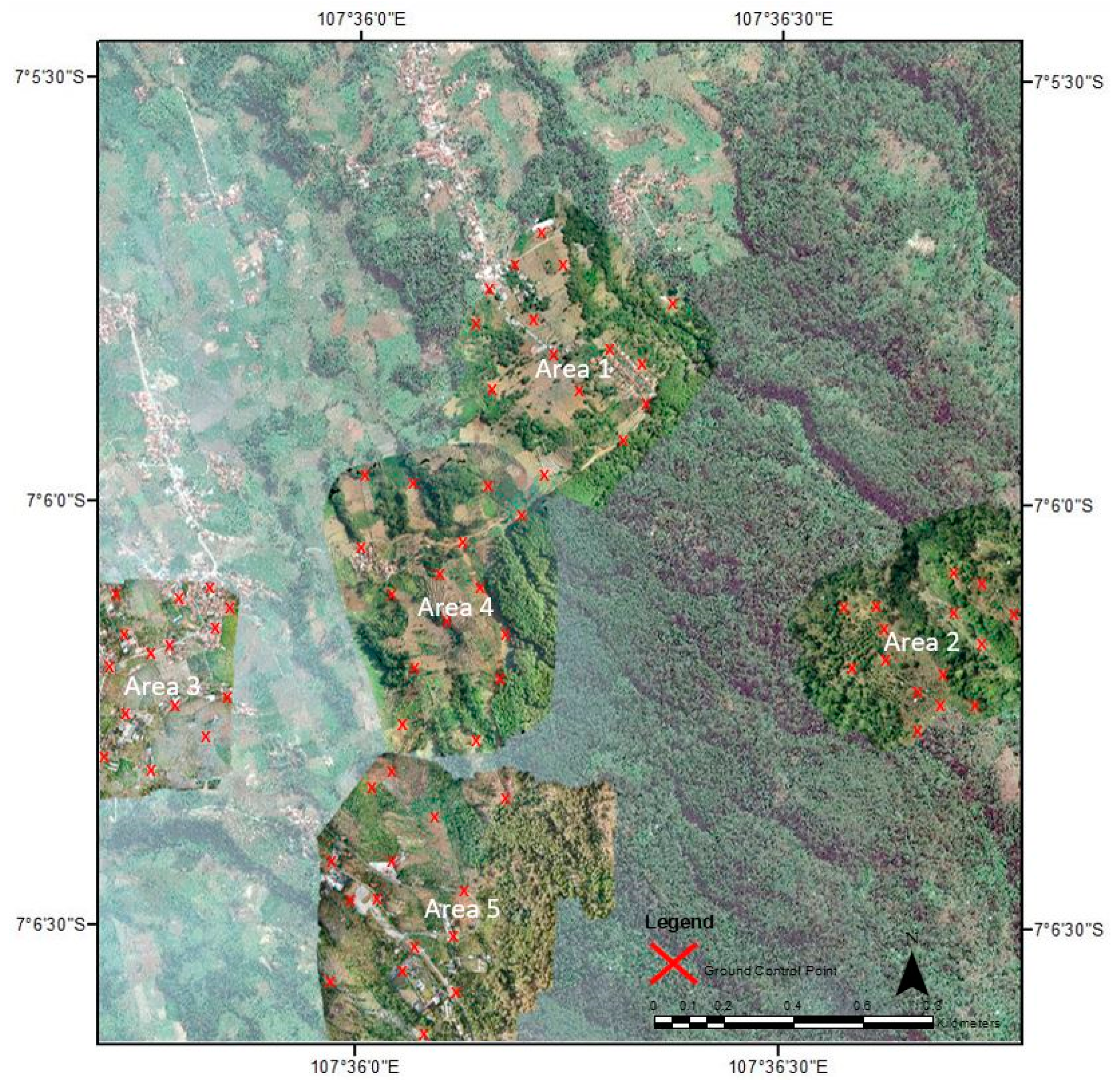
The aim of this research was to map coffee plantations based on multi-resolution, multi-temporal, and multi-sensor data using remote sensing; these data can be seen in Table 1.
In this research, we preprocessed images focusing on geometric, radiometric, and terrain corrections. All images were projected onto Universal Transverse Mercator (UTM) with WGS 84 Datum. Radiometric correction was also required for pan-sharpened GeoEye-1 and Sentinel 2. The dark object subtraction (DOS) atmospheric correction was applied for multi-temporal Sentinel 2 [36]. Next, the digital number (DN) of the pan-sharpened GeoEye-1 was converted to reflectance based on the GeoEye-1 corrections formula and calibration coefficients [37]. Another way of improving the classification of land cover in mountainous terrains consists of using terrain corrections [38]. In this research, the terrain correction method used was Minnaert correction [39]. Minnaert is a popular and widely used terrain correction method for mapping forest areas [40,41]. This equation requires information regarding the sun azimuth and elevation at the time of image acquisition, DEM, and the original image. The different spatial resolution of images was integrated by resampling data using the nearest neighbor to a grid cell-size equivalent to the highest resolution of data involved in this process. All images were resampled to 0.5 m.
We applied either NDVI or tasseled cap transformation to the multi-temporal Sentinel 2 images [42,43,44]. Multi-scale and multi-feature textures were chosen for analysis including entropy, mean, contrast, standard deviation, and correlation with window size 5 × 5, 15 × 15, and 25 × 25 derived from a green band of pan-sharpened GeoEye-1. In total, 29 variables were used in this research (Table 1). Normalization needs to be done due to the different range of images [45]. The dataset was transformed using the min-max normalization method by processing the minimum and maximum value of each attribute [46,47].
Before running the random forest algorithm, we had to set three parameters; which were: the number of trees, the number of variables predictor (mtry), and the number of minimum node sizes [48]. We varied these parameters across a wide range of values to achieve the best parameter combination (number of trees = 400 to 1000; the number of variables predictor: all variables and square root; minimum node size: 2 to 10). Next, we applied a random forest algorithm [18] using the best parameters to construct classification models by combining multi-sensor, multi-temporal, and multi-resolution remote sensing data from pan-sharpened GeoEye-1, Sentinel 2, and DEMfor mapping coffee plantations. Variable importance was also measured and models were created based on the most important variables. Each model was trained and validated with the reference data collected being based on aerial photographs and field surveys.

2.3. Field Surveys

Regarding the field surveys, we collected VHR aerial imagery data obtained from Unmanned Aerial Vehicle (UAV) platforms on 30 August 2019. These were used as references in making training and testing points. The VHR aerial imagery data were collected at five different locations (Figure 2). The locations were chosen based on the variations in land cover and were expected to represent coffee plantations in the research area. Both DJI Phantom 4 pro and Mavic 4 pro have same specifications, including the sensor of 20 MP camera resolution, 1” CMOS, a spectral resolution of 5472 × 3648 pixels, a mean ground sample distance (GSD) of 3 cm/pixel for a flight height of 100 m above take-off level with 80% overlap, and have three visible bands (red, green, and blue). The VHR aerial imagery was carried out using Agisoft Metashape 1.6 [49] with a total of 120 photos in Area 1; 92 photos in Area 2; 546 photos in Area 3; 223 photos in Area 4, and 573 photos in Area 5. Several steps were taken in the process: (1) creating a flight plan, (2) aligning photos in order to equalize the same points between photos (matching points) which were then used as tie points to build a point cloud, (3) building a dense cloud to interpolate the point cloud from aligning photos to form an object, (4) employing building mesh to build a 3D model of the resulting VHR aerial imagery. We also performed distortion geometric correction by using a ground control point (GCP). The number of GCP for each UAV image is 15 GCP which is distributed evenly. The accuracy of the geometric corrections is indicated from the Root Mean Square Error (RMSE) value per pixel in the image. In general, these values are less than one pixel. If the value is greater than one, there is a possibility that the image is still distorted [50]. The RMSE of UAV image in each area can be seen in Table 2.

2.4. Land Cover Classification Scheme

Based on existing land cover in the research area, we determined ten land cover for classification due to the differences in land cover patterns and gradients in elevation (Table 3). We used a balanced sample of 400 pixels to each class as training samples [50] and 150 pixels to each class as testing samples in the classification model [51]. The number of testing samples is in keeping with recommendations from ISO 19157:2013 [52]. All samples obtained from field surveys and VHR aerial imagery (3 cm spatial resolution) were interpreted. A stratified random sampling approach was then applied. Stratified random sampling is a probability sampling technique wherein the sampling is carried out randomly by first dividing the population into strata since the elements of populations are not proportionally stratified [53,54].

2.5. Textural Analysis

We applied textural features using the Gray Level Co-occurrence Matrix (GLCM) which is a a statistical method used to extract the second order statistical textural features from the given image [55]. These textural features were extracted from a matrix containing gray level occurrence frequencies (digital numbers) of pairs of pixels at fixed relative positions in an image. GLCM has some advantages including easily done and has been shown to give very good results in a large field of applications [56]. Furthermore, Maillard shows that GLCM gives better results than semi-variogram and the Fourier spectra for simple situations where the textures are visually easily separable [57]. Therefore, GLCM was chosen because this method outperforms other methods in distinguishing textures [58,59]. Some studies show that the integration of spectral and textural features using GLCM improves classification accuracy [30,31,55,60,61].
In this research, five textural features were applied: contrast, correlation, standard deviation, entropy, and mean [25,29,62]. These features were chosen due to the strong correlation frequently reported between many of the features, can reduce the complexity of the algorithm, and are more efficient than using all the features [29]. The textures were derived from the green band of pan-sharpened GeoEye-1 image as variables in coffee plantation discrimination. In addition, green band is useful to determine vegetation types, vigor, and to differentiate between healthy and unhealthy plants [63]. According to Karjono [64], a classification based on a combination of several windows (multi-scale texture) provides higher accuracy than using only one window size (single-scale texture). Rodriguez-Galiano et al. [21] also show that the use of multi-scale texture in random forests increases the accuracy by 30% in some categories, which is better than when only using a single-texture window size. By referring to previous research Franklin et al. [65], three different window sizes of 5 × 5, 15 × 15, and 25 × 25 were obtained. These windows size were obtained based on semivariograms and then were applied to diagonal (1, 1) orientations.
Entropy   =   i = 0 N 1 j = 0 N 1 P i , j ln P i , j
Mean   =   i = 0 N 1 j = 0 N 1 iP i , j
Standard   Deviation   =   i = 0 N 1 j = 0 N 1 P i , j ( i μ i ) 2
Contrast   =   i = 0 N 1 j = 0 N 1 P i , j ( i j ) 2
Correlation   =     i = 0 N 1 j = 0 N 1 ( i μ i ) ( j μ j ) σ i σ j P i , j
where P i , j is the ( i j ) th entry in GLCM, μ i is the mean vector of class i with the formula μ i = i j iP i , j , μ j   is the mean vector of class j with the formula μ j = i j jP i , j , σ i is standard deviations of P i with formula σ i = i j ( i μ i ) 2 P i , j , and σ j is standard deviations of P j with formula σ j = i j ( j μ j ) 2 P i , j   .

2.6. Derivation of Topography Data

The integration of topographical data and remote sensing imagery can improve the accuracy of classifications in mapping coffee plantations. Topographical indexes including elevation, slope, and aspect were widely used by researchers for mapping coffee plantations [7,13,14,66]. According to Kelley et al. [14], adding these topographical variables (elevation, slope, and aspect) in mapping coffee plantations increases classification accuracy by 7.8–20.1%.
In this study, all topographical data layers (elevation, aspect, and slope) were derived from DEMNAS data provided by the Geospatial Information Agency-Indonesia (BIG). DEMNAS is an elevation model with 0.27 arc-second (8.3 m) resolution (Tides.big.go.id), which is derived from various data sources: Interferometric Synthetic Aperture Radar (IFSAR) at 5-m resolution, TerraSAR-X at 5-m resolution, and Advanced Land Observing Satellite-Phased Arrayed L-band SAR (ALOS PALSAR) at 11.25 m resolution. It adds Masspoint data from stereo-plotting results. This dataset contains one band for elevation.

2.7. Derivation of Vegetation Index

The vegetation index is the transformation of two or more spectral bands from different electromagnetic waves to produce information about land cover change and green biomass [67]. Normalized Difference Vegetation Index (NDVI) is the most popular vegetation index [44]. We applied NDVI to the multi-temporal Sentinel 2 for mapping coffee plantations, given its success in improving the accuracy of coffee plantation mapping [7,14,66]. According to Cordero-Sancho and Sader [7], mapping coffee plantations using a combination of NDVI and DN produces better accuracy results than when using only DN. Hailu et al. [66] classified coffee in an agroforestry system using SPOT 5 images. The results of this research indicate that NDVI is the best variable for land cover classification as it produces an overall accuracy of 87.8%.
NDVI   =   NIR RED NIR + RED
where NIR is reflection in the near-infrared spectrum, RED is reflection in the red range of the spectrum.

2.8. Tasseled Cap Transformation

The tasseled cap algorithm was invented by Kauth and Thomas [68] who extracted it from the Landsat MSS; the tasseled cap produces three functions consisting of brightness, greenness, and yellowness. In 1984, Crist and Cicone further developed this algorithm by changing the yellowness index to the wetness index. Tasseled cap has been used for monitoring agricultural land [69], plant health [70], and detecting changes in land cover [71]. Kelley et al. [14] used tasseled cap from Landsat 8 OLI data as additional data for the identification of coffee plants in agroforestry systems. The results of their research show that the use of tasseled cap improves accuracy in the mapping of coffee plantations.
Following previous research Kelley et al. [14], we applied tasseled cap as ancillary data to a multi-temporal Sentinel 2 image to obtain an index of brightness, greenness, and wetness. Tasseled cap was used in this research because this transformation compresses information from a number of bands and minimizes information loss; it is suitable for application in areas of high complexity (heterogeneous) [72]. We used coefficient values following the Sentinel 2 reflectance data provided by Shi and Xu [43] which is this specific coefficient derived from PCP method can effectively enhance brightness, greenness, and wetness characteristics of the Sentinel-2 multispectral at sensor reflectance. In addition, these coefficients can accurately interpret the corresponding biophysical characteristics of land cover better than coefficient derived by Nedkov [43]. These coefficients can be seen in Table 4.

2.9. Optimization Parameter of Random Forest Algorithm

Before constructing the random forest classification, we investigated the best random forest parameter to obtain an optimal classification result. The parameters tested in this research were: tree, mtry, and minimum node size [48]. Studies have used 100 trees [73], 500 trees [14,74,75], and 1000 trees [76]. Du et al. [19] indicate that trees between 10 and 200 had no influence on classification accuracy. Some researchers also maintain that 300 is the minimum number of trees needed to retain accuracy [74,77]. In this research, trees were tested ranged from 400 to 1000.
Mtry is the number of variables used in splitting each node. The variables used for splitting each tree were randomly selected to minimize the correlation between the trees [21,74]. According to Breiman [18], mtry can be calculated using the √k, where k is the total number of variables. Some researchers have also followed this formula [78,79,80]. In this research, we tested both mtry = √k [18] and mtry = k (all variables). The minimum node size is the minimum number of samples required for each node splitting. Breiman [18] suggest using 2 minimum node sizes for all the trees in the land cover classification to allow them to grow fully without pruning. In this research, the minimum node sizes tested ranged from 2 to 10. To obtain optimal parameters, a random forest classification model was constructed based on the results of a cross combination of all the parameters. These cross combinations parameters produce 126 classification models. Random forest classification was run using the Vigra tool in SAGA 7.6.2 software [81].

2.10. Mapping Coffee Plantations Based on a Full Model Approach

We constructed a random forest classification algorithm for mapping coffee plantations derived from pan-sharpened GeoEye-1, multi-temporal Sentinel 2, and DEM data (total of 29 variables) as the input image denoted as model 5 (M5) using the best random forest parameters. We then compared the classification accuracy produced by a model derived from using 29 variables with the other four-classification model to determine the effect of textures, spectral bands, topography, NDVI, and tasseled cap for mapping coffee plantations. These models can be seen in Table 5.

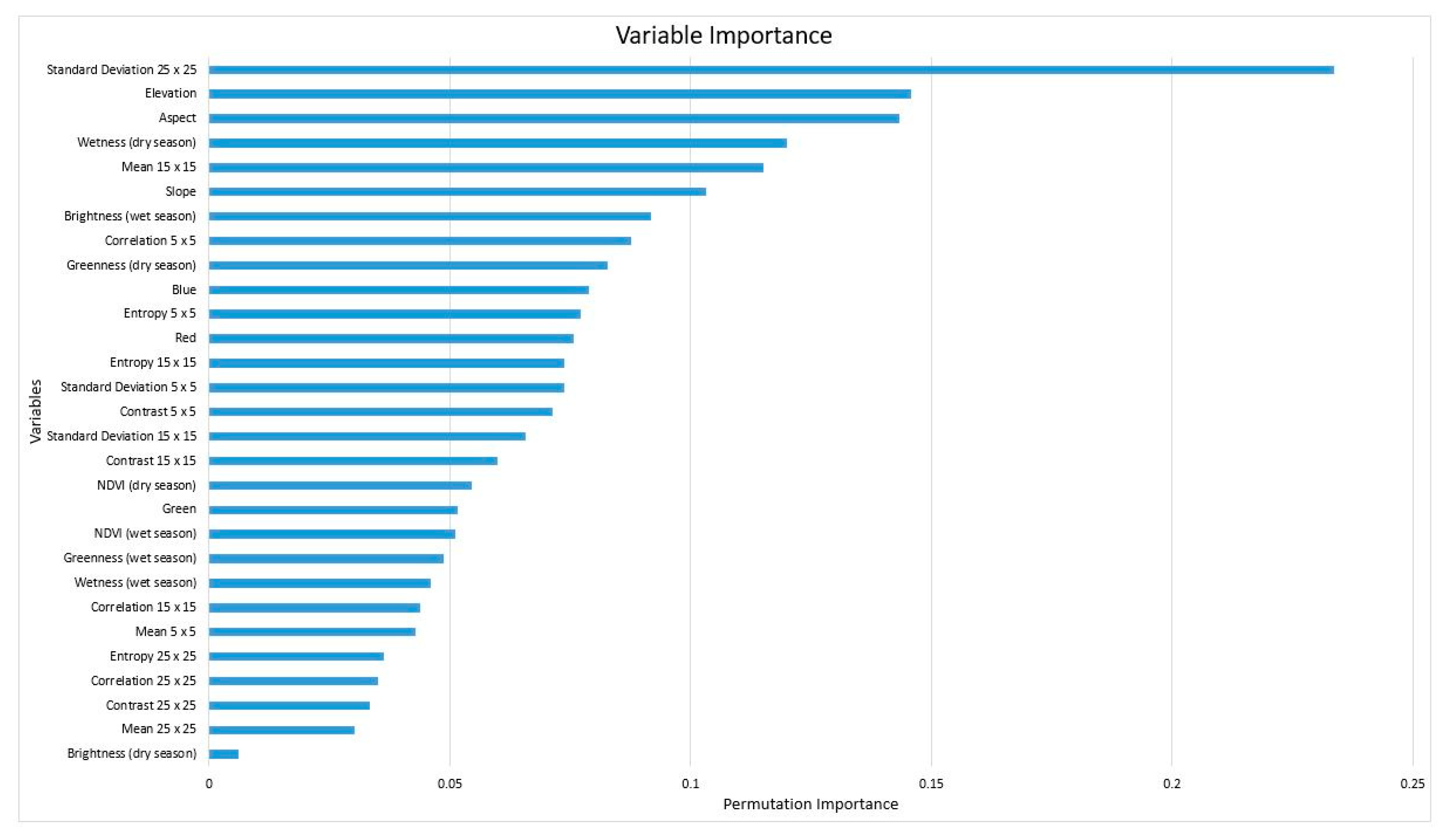
2.11. Variables of Importance

In total, 29 variables were obtained from pan-sharpened GeoEye-1, multi-temporal Sentinel 2, and DEM which were used for mapping coffee plantations (Table 1). It is important to know the influence of each variable on the classification result. The importance of the variables is measured based on the value of permutation or the mean decrease accuracy (MDA). In this process, random permutations of the variables at the out of the bag (OOB) value were measured. OOB error is a method for validating the random forest model. The accuracy change value was then measured to determine the variable of importance. Based on the value of the variable of importance, the most important variables were then selected to produce a more efficient classification model which was then used for mapping coffee plantations in the research area.

2.12. Accuracy Assessment of Classification Model

Accuracy assessment was used to compare the result of each classification model with the ground truth. Following previous research, the accuracy of each classification was evaluated using a confusion matrix [82]. This approach can assist in identifying misclassifications between different land cover and potential sources of error. The percentage of the classification accuracy results was seen from the following values: kappa statistics, overall accuracy, user accuracy, and producer accuracy [83]. Ideally, all non-diagonal elements in the matrix should be zero, which means that there are no deviations in the matrix [63].
Kappa   statistics   =   N i = 1 n Xii i = 1 n Xi + ( X + i )   N 2 i = 1 n Xi + ( X + i ) ×   100 %
Overall   Accuracy   =   i = 1 n Xii N   ×   100 %
Users   Accuracy   =   Xii X + i   ×   100 %
Producer   Accuracy   =   Xii X + i   ×   100 %
where N = the number of all pixels used for observation, R = the number of rows in the error matrix (number of classes), Xii = Diagonal values of the contingency matrices of row i and column i, X + i = column pixel number i, and Xi + row pixel number i.

3. Results

3.1. Parameter Optimal in Random Forest Algorithm
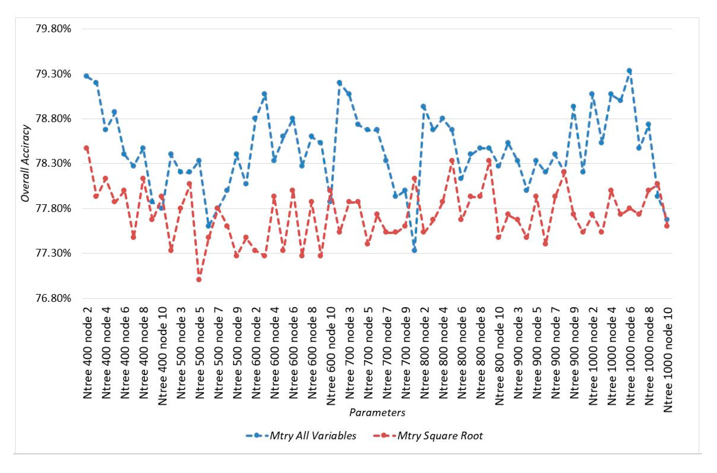
3.1.1. Mtry

The use of mtry = k (all variables) was significant in producing higher accuracy than when using mtry = √k (square root) (Figure 3). The highest accuracy derived by the parameter combination of mtry = k, tree = 1000 and minimum node size = 6 produced overall accuracy and kappa statistics of 79.333% and 0.774, respectively; whereas, the lowest accuracy obtained by the parameter combinations of mtry = √k, tree = 500 and minimum node size = 5 produced overall accuracy and kappa statistics of 77% and 0.744, respectively. The use of mtry = k (all variables) and mtry = √k (square root) produced an average of the overall accuracy of 78.450% and 77.740%, respectively.

3.1.2. Tree

The average of overall accuracy obtained by each tree can be seen in Table 6. The highest overall accuracy obtained by using tree = 1000 produced an overall accuracy of 78.644%. Nevertheless, the relative use of trees numbering from 400 to 1000 did not provide a significantly fluid increase in accuracy. The average overall accuracy of each tree is in the range of 78%. The uses of the tree did not significantly influence the classification accuracy compared to the uses of mtry.

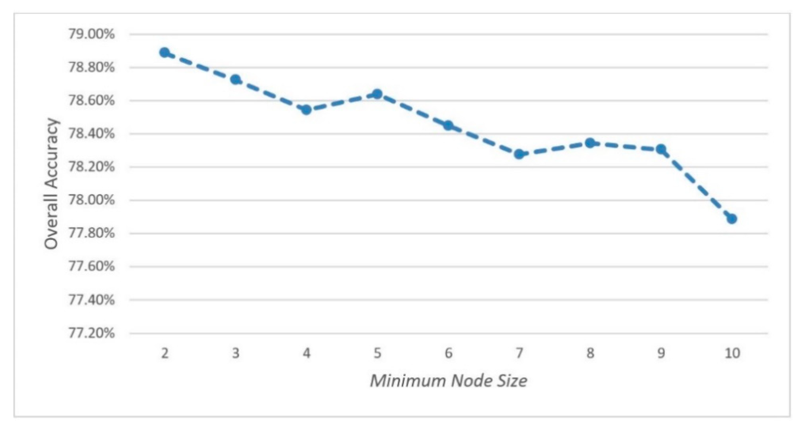
3.1.3. Minimum Node Sizes

Figure 4 shows an average of overall accuracy obtained from using minimum node sizes 2 to 10. It has been shown that using minimum sizes 2 to 10, produced a decreasing overall accuracy which is proportional to the increasing number of minimum node sizes used. The node size parameter specified the minimum number of samples in each node. The more samples of each node, the lower the accuracy resulted. The highest overall accuracy of 78.886% was produced by using two minimum samples in each node; whereas, using 10 minimum node sizes produced the lowest overall accuracy of 77.886%.
The determination of minimum node size is used as a control in constructing trees. Decreasing the tree size will be controlled by setting a higher node size value. Trees with the lowest minimum node size (set to 2) will be allowed to grow fully until the smallest sample size of each node is obtained; on the other hand, if a larger minimum node size is used, tree growth will be limited, indicating that the tree must be pruned. This minimizes the possibility of overfitting due to the complexity of the resulting model.

3.1.4. Combination of All Parameters

A total of 126 classification models were applied to obtain best parameter combination using all variables (29 variables) and the same training points. The highest and lowest overall accuracy percentages obtained for each model can be seen in Table 7.
The highest accuracy obtained by combining the parameters of mtry = k, tree = 1000, and minimum node = 6 produced an overall accuracy of 79.333%; whereas, the lowest accuracy obtained by the combination of parameters mtry = √k, tree = 700, and minimum node size = 10 produced an overall accuracy of 77.333%. Based on Figure 4, an average of the overall accuracy of minimum node size 2 provides the highest accuracy of 78.886%. Meanwhile, the combination parameters of tree = 1000, mtry = k, and minimum node size = 6 produces higher overall accuracy than the using of minimum node size 2 which is 79.333%. It indicated that producing the best accuracy requires a combination of parameters used as input classifications. Therefore, the parameter combination of mtry = k, tree = 1000, and minimum node = 6 used as random forest parameters for mapping coffee plantations.

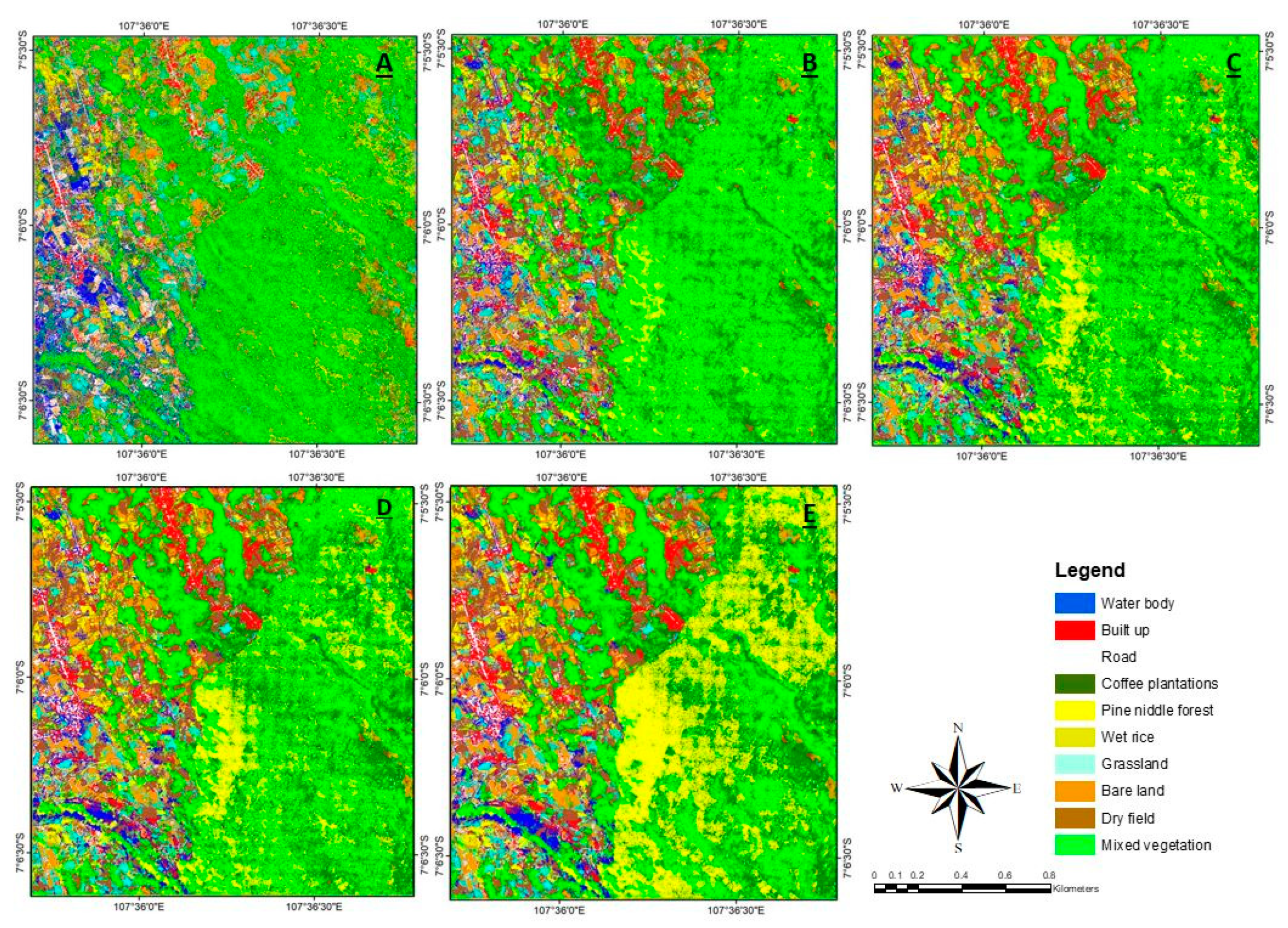
3.2. Distribution of Coffee Plantations

The spatial distribution of coffee plantations which were derived from the full set of pan-sharpened VHR image, topography, texture, multi-temporal NDVI, and multi-temporal tasseled cap (M5) using the random forest algorithm (mtry = k, tree = 1000 and minimum node = 6) produced overall accuracy, kappa statistics, producer accuracy and user accuracy of 79.333%, 0.774, 92.000%, and 90.790%, respectively. The results of the confusion matrix of classification accuracy produced by this model can be seen in Table 8.
The accuracy of the classification results (rows) of all variables against the reference data (columns) can be seen in Table 8. The confusion matrix denotes overall accuracy (OA), kappa statistics, user accuracy (UA), and producer accuracy (PA). This model shows good performance in mapping coffee plantations (class 4) as confirmed by high producer and user accuracy rates of 90.79% and 92%, respectively. In contrast, classes 1 (water body), 2 (built-up), and 3 (road) produce a relatively low value of producer accuracy and user accuracy. This is due to all variables used as input classification model in this study indeed the variables for mapping coffee plantations, not for the other class. Based on the classification that was done using all the variables (29 variables), we compared this with four other models (Table 9) to investigate the influence of textures, spectral bands, topography, NDVI, and tasseled cap for mapping coffee plantations. A total of five models were tested in this research. The results of the overall classification accuracy produced from the entire model can be seen in Table 9, while the classification results can be seen in Figure 5.
The classification accuracy obtained by all models can be seen in Table 9. These data show a trend of increasing the accuracy of land cover classification in line with the increasing number of variables. The use of the M5 model (RGB + Texture + Elevation + NDVI + Tasseled Cap) significantly provides the highest overall accuracy for mapping coffee plantations. In the M1, the classification model derived from the spectral data of the pan-sharpened GeoEye-1 (the red, green, and blue bands) produced the lowest accuracy compared to the other models. Applying this model produced overall accuracy, kappa statistics, producer accuracy, and user accuracy of 58.540%, 0.530, 65.888%, and 59.899%, respectively. The application of a textural variable (M2) in the random forest classification model showed a significant increase (14.6%) in overall accuracy. An overall improvement accuracy of 2.21% was also reported; while producer accuracy increased by 2.58% and user accuracy increased by 2.37% when topographical variables (elevation, aspect, and slope) were added to this research (M3). On the other hand, the M4 model shows that the use of the NDVI variable has the lowest improvement in accuracy, only 0.51%. Producer accuracy also decreased by 1.59% while user accuracy increased by 2.56%. Nevertheless, the addition of multi-temporal data; namely, the NDVI vegetation index and the tasseled cap, increased the overall accuracy of mapping coffee plantations. The addition of multi-temporal tasseled cap showed an increase in accuracy of 3.47%. Producer accuracy increased by 1.33% and user accuracy increased by 3.61%.

3.3. Mapping Coffee Plantations Using Variables of Importance

As mentioned above, although random forests can be used for dimensional data, the classification results can improve accuracy only when using the most important variables. The variable importance obtained by the full model can be seen in Figure 6.
The variables of importance derived by the full set of RGB + Texture + Elevation + NDVI + Tasseled cap model using random forest (mtry = k, tree = 1000, and minimum node size = 6) can be seen in Figure 6. Based on this data, the five most important variables are: standard deviation 25 × 25, elevation, aspect, wetness index (dry season), and mean 15 × 15. The brightness (dry season) is the variable with the lowest level of importance. Several textural variables with a size of 25 × 25 also have low importance. The results show that the topographical effects (aspect, elevation, and slope) had a relatively large influence. This is due to coffee plants growing on mountain slopes, which means that topographical influences greatly contribute to differentiating coffee trees from other land covers. Furthermore, we selected a model based on the median and the mean value of permutation importance, as well as ±5 variables from the median. Therefore, the 10 most important, 12 most important, 15 most important and 20 most important variables were selected. The classification results can be seen in Table 10.
The classification accuracy obtained by variations of the most important variables can be seen in Table 10. This data indicates that the use of the 12 most important variables produced the highest overall accuracy, kappa statistics, producer accuracy, and user accuracy percentages of 79.333%, 0.774, 91.33%, and 84.57%, respectively. The 12 most important variables are the standard deviation of 25 × 25, elevation, aspect, wetness index (dry season), mean 15 × 15, slope, brightness (wet season), correlation 5 × 5, greenness (dry season), blue channel, entropy 5 × 5, and the red channel. This model provides the same overall and kappa statistics using all variables, but with the different producer and user accuracy.

4. Discussion

4.1. Parameter of Random Forest Classifications

In total, 126 model classifications were used for selecting the best parameter in constructing random forest classifications. Mtry is the number of variables selected randomly when splitting nodes. Mtry is used as a control in the variable selection process, indicating that the smaller the mtry value, the stronger the randomization will be. On the other hand, there is no randomization taking place in the split selection when using all the variables, indicating that all variables are allowed in splitting. In this research, the use of all variables (29 variables) significantly produced higher accuracy than the method proposed by Breiman [18]; namely, √k. Based on these results, it can be seen that the fewer variables used for splitting, the lower the accuracy; whereas, the more variables used for splitting, the better the produced accuracy will be. This is also in line with research conducted by Gao [27], who found that the higher the number of mtries, the higher the produced accuracy.
The use of trees from 400 to 1000 does not provide a significant and fluid increase in accuracy. This is following the previous researches [84,85] who stated that tree has no significant influence on classification accuracy compared to mtry. In this research, the best accuracy was obtained by using the tree = 1000 which produced an average of overall accuracy of 78.64%. Although Gao [27] report that the use of tree 500 obtained high accuracy; however, the use of tree 500 in this research obtained the lowest accuracy. This is due to the different morphological conditions in the research area [86].
The lower number of samples in each node will provide better accuracy, otherwise, the more samples tends to decrease the accuracy. This research follows the recommendation made by Breiman [18], who indicates that the use of a minimum node size 2 will give good classification results. This is due to the small minimum node size, causing the tree to continue splitting until the nodes are truly pure; however, this condition will result in overfitting. Therefore, it is necessary to analyze the parameter combination.
Although an average of overall accuracy of minimum node size 2 provides the highest accuracy, that of 78.886% (Figure 4), the combination of each tree for each minimum node size gives a higher percentage of accuracy; namely, 79.333% as a result of the parameter combination of tree = 1000, mtry = k, and minimum node size = 6 (Table 7). Based on the results that were obtained, it can be concluded that to obtain the best accuracy it is necessary to cross-combine all of the mtry parameters, the minimum node size, and the number of trees; these are then used as input random forest parameters in classifying.

4.2. Distribution of Coffee Plantations

In this section, the effects of increasing the variables for a particular model are analyzed. The classification used only the spectral data from the pan-sharpened GeoEye-1 which produced the lowest accuracy compared to other models. The results show that this model cannot discriminate coffee plants from other crops, including pine needle trees; due to the research area being influenced by topographical effects and spectral similarities with other vegetation [87]. This is in line with research conducted by Mukashema [88] who found that using only spectral of high-resolution images is insufficient for mapping coffee plantations accurately. Therefore, additional variables are needed to differentiate coffee plants from other land cover classifications.
The addition of textural variable in the random forest classification model significantly increases overall accuracy by 14.6%. This is in line with previous research conducted by [65,89] that textural variables have high contribution to accuracy. On the other hand, it was difficult to distinguish coffee plantations from other vegetation in an area that has different elevations and slopes. Therefore, by including topographical variables (elevation, aspect, and slope) it is possible to distinguish coffee plants from mixed vegetation that grow at different elevations and slopes. In areas with low elevation, coffee plants can be distinguished from mixed vegetation. By adding topographical variables, an increase in the overall accuracy of 2.21% was seen, along with producer accuracy of 2.58%, and user accuracy of 2.37%. The improvement in accuracy obtained by adding topographical data in mapping coffee plantations is also noted by previous research [14].
This research also indicates that the use of NDVI variable data shows the lowest increase in overall accuracy, that of 0.51% (M4). This model is comparable with prior research [14]. Kelley [14] indicate that the use of NDVI variables increases overall accuracy by only 1%. However, the addition of multi-temporal data; namely, the NDVI vegetation index and the tasseled cap obtained by M4 and M5 models, increases the overall accuracy of mapping coffee plantations. The addition of tasseled cap multi-temporal data showed an increase in overall accuracy of 3.47%, producer accuracy of 1.33%, and a user accuracy increase of 3.61%.
The most significant finding of this research is that the highest accuracy was achieved by full models (integration of pan-sharpened GeoEye-1, multi-temporal Sentinel 2, and DEM), using the best random forest parameters (mtry = k, tree = 1000, and minimum node size = 6). This model achieved an overall accuracy of 79.333% and a kappa statistics of 0.774. The overall accuracy obtained by this research was significantly higher than that of Sancho [7] who reported 65% accuracy, and the 76.7% accuracy reported by Huerta [11]. The overall accuracy of land cover mapping by this model is lower than that achieved by Kelley [14], which is 90.5%. This is probably due to differences in the image resolution used (30 m), the scale of the area under research (regional), and the use of precipitation data. In this research, precipitation data were not used for two reasons. The first reason is because of the unavailability of this data for the research area. Precipitation data currently available is CHIRPS with a resolution of 0.05° (5 km), while the research area is 4 km. Secondly, precipitation data contributes only slightly to the overall accuracy, which is 1%; otherwise, it reduces coffee user accuracy to 4.4% [14].
This research integrated pan-sharpened GeoEye-1, multi-temporal Sentinel 2, and DEM using random forest classification (mtry = k, tree = 1000, and minimum node size = 6) which show good results in mapping coffee plantations as evidenced by high producer and user accuracy rates of 92% and 90.79%, respectively. These high values indicate that classification techniques using the random forest algorithm can be used for mapping coffee plants and land cover in agroforestry areas. In this research, producer accuracy and user accuracy were significantly higher than that reported by Sancho [7] who reported a user accuracy of 79.3% and a producer accuracy of 75%; Kelley [14] reported 82.1% user accuracy and 80% producer accuracy. However, some misclassifications between coffee and mixed vegetation still occurred. This is due to the unavoidable spectral similarity of coffee plants to other vegetation.

4.3. Important Variables

Classification results achieved from 12 important variables indicate that the random forest algorithm is a reliable approach for improving efficiency in classification. The use of the 12 most important variables provides reliable overall accuracy, kappa statistics, producer accuracy, and user accuracy which are 79.333%, 0.774, 91.333%, and 84.570%, respectively. This model achieved the same overall accuracy by using all the above-mentioned variables. This research is also in line with that of Gao [27], who also found that the random forest algorithm can reduce the variables. The model was derived by applying the 12 most important variables: standard deviation 25 × 25, elevation, aspect, wetness (dry season), mean 15 × 15, slope, brightness (wet season), correlation 5 × 5, greenness (dry season), blue, entropy 5 × 5, and red. The most important variable in this research is the standard deviation 25 × 25. Previous studies also suggest that the use of textures can improve accuracy [27,65].
Topographical effects (aspect, elevation, and slope) show higher importance in this model due to the fact that coffee plants mostly grow on mountain slopes so that topographical effects greatly contribute to differentiating coffee from other land covers. Table 9 shows that adding topographical effects (aspect, slope, and elevation) significantly increases accuracy in discriminating coffee plantations. However, the multi-temporal NDVI variable is relatively weak. This is in accordance with the results described in Table 9; i.e., the addition of the NDVI variable in the classification model only obtained an increase in accuracy of 0.5%. In this research, we conclude that the NDVI variable provides a minor contribution. This is because NDVI is a vegetation index that is affected by canopy density, chlorophyll content, and useful for measuring neighborhood greenness [90]. Whereas, the coffee plantation has spectral similarities with other plantations and has trees different characteristics in different seasons [87]. This result is also in line with Kelley [14] who state that the use of NDVI variables increases overall accuracy by only 1%.

5. Conclusions

Mapping coffee plantations using satellite imagery is particularly challenging due to spectral similarities with other plantations. Hence, the classification scheme for mapping coffee plantations requires proper understanding of the data used on the field. This research focuses on the suitability of integrating pan-sharpened GeoEye-1, multi-temporal Sentinel 2, and DEM using random forest algorithm for coffee plantation mapping in the agroforestry system. The spectral band as well as textural variables extracted from pan-sharpened GeoEye-1, multi-temporal NDVI, and tasseled cap extracted from Sentinel 2, and topographical effects (slope, aspect, and elevation) extracted from DEM were used as input in a random forest classification model. In total, 29 variables were used for constructing a random forest classification using the best parameters combination (mtry = k, tree = 1000, and minimum node size = 6). This model indicates that the integration of pan-sharpened GeoEye-1, multi-temporal Sentinel 2, and DEM shows the best performance in mapping coffee plantations in the agroforestry system and provides overall accuracy of kappa statistics, producer accuracy, and user accuracy of 79.333%, 0.774, 92.000%, and 90.790%, respectively. High classification accuracy was also achieved by using the most 12 important variables: standard deviation 25 × 25, elevation, aspect, wetness (dry season), mean 15 × 15, slope, brightness (wet season), correlation 5 × 5, greenness (dry season), blue, entropy 5 × 5, and red. This combination of variables provides overall accuracy of: kappa statistics, producer accuracy, and user accuracy of 79.333%, 0.774, 91.333%, and 84.570%, respectively. Our results indicate that using a random forest algorithm can increase efficiency in mapping coffee plantations in the agroforestry system when using only the 12 most important variables. In future work, we hope to explore these random forest parameters and variables in various other coffee-producing terrain and further develop this research, using both spatial and temporal high resolution for increasing accuracy in mapping coffee plantations.

Author Contributions

A.T., K.W., T.M.S., A.B.H. and S.D., conceived and designed the experiments; A.T., T.M.S., K.W. and L.F.Y. performed the experiments; A.T., T.M.S., K.W. and L.F.Y. investigations; A.T., M.F.G. and A.B.H. analyzed the data; A.T. and T.M.S. constructed the model; A.T., T.M.S. and S.D. validated the model; A.T. wrote the paper; and all authors read the paper and provided revision suggestions. All authors have read and agreed to the published version of the manuscript.

Funding

This research received no external funding and the APC was funded by Center for Remote Sensing, Institut Teknologi Bandung-Indonesia.

Acknowledgments

The authors would like to thank Digital Globe for providing data support for this research. The authors would also like to thank the Department of Geomatics and Engineering of Bandung Institute of Technology (ITB), the Center for Remote Sensing-Institut Teknologi Bandung (ITB), Indonesia, Institut Teknologi Nasional, Universitas Lampung, and KJSKB Ketut Tomy Suhari for their support. Special thanks also to Yohannes Dian Aditya, M. Ali, Haikal, Efrila Aji, Sapta Yonda, and Nilton for assisting in the field survey.

Conflicts of Interest

The authors declare that there is no conflict of interest.

References

  1. Supriadi, H.; Pranowo, D. Prospek pengembangan agroforestri berbasis kopi di Indonesia. Perspektif 2016, 14, 135–150. [Google Scholar]
  2. ICO. Exports of All Forms of Coffee by Exporting Countries to All Destinations. 2019. Available online: http://www.ico.org (accessed on 12 September 2019).
  3. FAO. Food and Agriculture Organization of the United Nations: FAOSTAT Statistical Database. Available online: http://www.fao.org/faostat/en/#data (accessed on 30 July 2020).
  4. ICO. Historical Data. 2017. Available online: http://www.ico.org (accessed on 6 June 2017).
  5. Lu, Y.C.; Daughtry, C.; Hart, G.; Watkins, B. The current state of precision farming. Food Rev. Int. 1997, 13, 141–162. [Google Scholar]
  6. LeBoeuf, J. Practical applications of remote sensing technology—An industry perspective. HortTechnology 2000, 10, 475–480. [Google Scholar]
  7. Cordero-Sancho, S.; Sader, S.A. Spectral analysis and classification accuracy of coffee crops using Landsat and a topographic-environmental model. Int. J. Remote Sens. 2007, 28, 1577–1593. [Google Scholar]
  8. Martínez-Verduzco, G.C.; Galeana-Pizaña, J.M.; Cruz-Bello, G.M. Coupling community mapping and supervised classification to discriminate Shade coffee from Natural vegetation. Appl. Geogr. 2012, 34, 1–9. [Google Scholar]
  9. Dos Santos, J.A.; Gosselin, P.-H.; Philipp-Foliguet, S.; Torres, R.d.S.; Falao, A.X. Multiscale classification of remote sensing images. IEEE Trans. Geosci. Remote Sens. 2012, 50, 3764–3775. [Google Scholar]
  10. Souza, C.G.; Arantes, T.B.; Carvalho, L.M.T.d.; Aguiar, P. Multitemporal variables for the mapping of coffee cultivation areas. Pesqui. Agropecuária Bras. 2019, 54, e00017. [Google Scholar]
  11. Ortega-Huerta, M.A.; Komar, O.; Price, K.P.; Ventura, H.J. Mapping coffee plantations with Landsat imagery: An example from El Salvador. Int. J. Remote Sens. 2012, 33, 220–242. [Google Scholar]
  12. Langford, M.; Bell, W. Land cover mapping in a tropical hillsides environment: A case study in the Cauca region of Colombia. Int. J. Remote Sens. 1997, 18, 1289–1306. [Google Scholar]
  13. Arias, S.B. Using Image Analysis and GIS for Coffee Mapping; McGill University Libraries: Montreal, QC, Canada, 2007. [Google Scholar]
  14. Kelley, L.C.; Pitcher, L.; Bacon, C. Using Google Earth engine to map complex shade-grown coffee landscapes in Northern Nicaragua. Remote Sens. 2018, 10, 952. [Google Scholar]
  15. Schowengerdt, R.A. Remote Sensing: Models and Methods for Image Processing; Elsevier: Amsterdam, The Netherlands, 2006. [Google Scholar]
  16. Sisodia, P.S.; Tiwari, V.; Kumar, A. Analysis of supervised maximum likelihood classification for remote sensing image. In Proceedings of the International conference on recent advances and innovations in engineering (ICRAIE-2014), Jaipur, India, 9–11 May 2014; pp. 1–4. [Google Scholar]
  17. Lu, D.; Weng, Q. A survey of image classification methods and techniques for improving classification performance. Int. J. Remote Sens. 2007, 28, 823–870. [Google Scholar] [CrossRef]
  18. Breiman, L. Random forests. Mach. Learn. 2001, 45, 5–32. [Google Scholar] [CrossRef] [Green Version]
  19. Du, P.; Samat, A.; Waske, B.; Liu, S.; Li, Z. Random forest and rotation forest for fully polarized SAR image classification using polarimetric and spatial features. ISPRS J. Photogramm. Remote Sens. 2015, 105, 38–53. [Google Scholar] [CrossRef]
  20. Pal, M. Random forest classifier for remote sensing classification. Int. J. Remote Sens. 2005, 26, 217–222. [Google Scholar] [CrossRef]
  21. Rodriguez-Galiano, V.; Chica-Olmo, M.; Abarca-Hernandez, F.; Atkinson, P.M.; Jeganathan, C. Random Forest classification of Mediterranean land cover using multi-seasonal imagery and multi-seasonal texture. Remote Sens. Environ. 2012, 121, 93–107. [Google Scholar] [CrossRef]
  22. Sartono, B.; Syafitri, U.D. Metode pohon gabungan: Solusi pilihan untuk mengatasi kelemahan pohon regresi dan klasifikasi tunggal. Indones. J. Stat. Appl. 2010, 15, 1–7. [Google Scholar]
  23. Van Beijma, S.; Comber, A.; Lamb, A. Random forest classification of salt marsh vegetation habitats using quad-polarimetric airborne SAR, elevation and optical RS data. Remote Sens. Environ. 2014, 149, 118–129. [Google Scholar] [CrossRef]
  24. Cutler, D.R.; Edwards, T.C., Jr.; Beard, K.H.; Cutler, A.; Hess, K.T.; Gibson, J.; Lawler, J.J. Random forests for classification in ecology. Ecology 2007, 88, 2783–2792. [Google Scholar] [CrossRef]
  25. Stumpf, A.; Kerle, N. Object-oriented mapping of landslides using Random Forests. Remote Sens. Environ. 2011, 115, 2564–2577. [Google Scholar] [CrossRef]
  26. Ghosh, A.; Joshi, P.K. A comparison of selected classification algorithms for mapping bamboo patches in lower Gangetic plains using very high resolution WorldView 2 imagery. Int. J. Appl. Earth Obs. Geoinf. 2014, 26, 298–311. [Google Scholar] [CrossRef]
  27. Gao, T.; Zhu, J.; Zheng, X.; Shang, G.; Huang, L.; Wu, S. Mapping spatial distribution of larch plantations from multi-seasonal Landsat-8 OLI imagery and multi-scale textures using random forests. Remote Sens. 2015, 7, 1702–1720. [Google Scholar] [CrossRef] [Green Version]
  28. Coltri, P.P.; Zullo, J.; do Valle Goncalves, R.R.; Romani, L.A.S.; Pinto, H.S. Coffee crop’s biomass and carbon stock estimation with usage of high resolution satellites images. IEEE J. Sel. Top. Appl. Earth Obs. Remote Sens. 2013, 6, 1786–1795. [Google Scholar] [CrossRef]
  29. Aguilar, M.; Saldaña, M.; Aguilar, F. GeoEye-1 and WorldView-2 pan-sharpened imagery for object-based classification in urban environments. Int. J. Remote Sens. 2013, 34, 2583–2606. [Google Scholar] [CrossRef]
  30. Liu, J.; Liu, H.; Lv, Y.; Xue, X. Classification of high resolution imagery based on fusion of multiscale texture features. In Proceedings of the 35th International Symposium on Remote Sensing of Environment, Beijing, China, 22–26 April 2013; pp. 22–26. [Google Scholar]
  31. Hurni, K.; Hett, C.; Epprecht, M.; Messerli, P.; Heinimann, A. A texture-based land cover classification for the delineation of a shifting cultivation landscape in the Lao PDR using landscape metrics. Remote Sens. 2013, 5, 3377–3396. [Google Scholar] [CrossRef] [Green Version]
  32. Moreira, M.A.; Adami, M.; Rudorff, B.F.T. Análise espectral e temporal da cultura do café em imagens Landsat. Pesqui. Agropecuária Bras. 2004, 39, 223–231. [Google Scholar] [CrossRef]
  33. Jia, K.; Liang, S.; Zhang, N.; Wei, X.; Gu, X.; Zhao, X.; Yao, Y.; Xie, X. Land cover classification of finer resolution remote sensing data integrating temporal features from time series coarser resolution data. ISPRS J. Photogramm. Remote Sens. 2014, 93, 49–55. [Google Scholar] [CrossRef]
  34. Hunt, D.A.; Tabor, K.; Hewson, J.H.; Wood, M.A.; Reymondin, L.; Koenig, K.; Schmitt-Harsh, M.; Follett, F. Review of Remote Sensing Methods to Map Coffee Production Systems. Remote Sens. 2020, 12, 2041. [Google Scholar] [CrossRef]
  35. Camargo, Â.P.d.; Camargo, M.B.P.d. Definição e esquematização das fases fenológicas do cafeeiro arábica nas condições tropicais do Brasil. Bragantia 2001, 60, 65–68. [Google Scholar] [CrossRef] [Green Version]
  36. Chavez, P.S. Image-based atmospheric corrections-revisited and improved. Photogramm. Eng. Remote Sens. 1996, 62, 1025–1035. [Google Scholar]
  37. Kuester, M. Absolute Radiometric Calibration: 2016v0; Digital Globe: Westminster, CO, USA, 2017. [Google Scholar]
  38. Dorren, L.K.; Maier, B.; Seijmonsbergen, A.C. Improved Landsat-based forest mapping in steep mountainous terrain using object-based classification. For. Ecol. Manag. 2003, 183, 31–46. [Google Scholar] [CrossRef]
  39. Minnaert, M. The reciprocity principle in lunar photometry. Astrophys. J. 1941, 93, 403–410. [Google Scholar] [CrossRef]
  40. Riaño, D.; Chuvieco, E.; Salas, J.; Aguado, I. Assessment of different topographic corrections in Landsat-TM data for mapping vegetation types (2003). IEEE Trans. Geosci. Remote Sens. 2003, 41, 1056–1061. [Google Scholar] [CrossRef] [Green Version]
  41. Hantson, S.; Chuvieco, E. Evaluation of different topographic correction methods for Landsat imagery. Int. J. Appl. Earth Obs. Geoinf. 2011, 13, 691–700. [Google Scholar] [CrossRef]
  42. Nedkov, R. Orthogonal transformation of segmented images from the satellite Sentinel-2. Comptes Rendus De L’academie Bulg. Des. Sci. 2017, 70, 687–692. [Google Scholar]
  43. Shi, T.; Xu, H. Derivation of Tasseled Cap Transformation Coefficients for Sentinel-2 MSI At-Sensor Reflectance Data. IEEE J. Sel. Top. Appl. Earth Obs. Remote Sens. 2019, 12, 4038–4048. [Google Scholar] [CrossRef]
  44. Rousel, J.; Haas, R.; Schell, J.; Deering, D. Monitoring vegetation systems in the great plains with ERTS. In Proceedings of the Third Earth Resources Technology Satellite—1 Symposium, Washington, DC, USA, 10–14 December 1973; NASA SP-351. pp. 309–317. [Google Scholar]
  45. Patro, S.; Sahu, K.K. Normalization: A preprocessing stage. arXiv 2015, arXiv:1503.06462. [Google Scholar] [CrossRef]
  46. Al Shalabi, L.; Shaaban, Z.; Kasasbeh, B. Data mining: A preprocessing engine. J. Comput. Sci. 2006, 2, 735–739. [Google Scholar] [CrossRef] [Green Version]
  47. Han, J.; Pei, J.; Kamber, M. Data Mining: Concepts and Techniques; Elsevier: Amsterdam, The Netherlands, 2011. [Google Scholar]
  48. Probst, P.; Wright, M.N.; Boulesteix, A.L. Hyperparameters and tuning strategies for random forest. Wiley Interdiscip. Rev. Data Min. Knowl. Discov. 2019, 9, e1301. [Google Scholar] [CrossRef] [Green Version]
  49. Agisoft. Agisoft Metashape User Manual: Professional Edition, Version 1.5; Agisoft: St. Petersburg, Russia, 2019. [Google Scholar]
  50. Sevilla, C.G. Research Methods Slovin; Rex Print. Co.: Quezoncity, Philippines, 2007. [Google Scholar]
  51. Fitzpatrick-Lins, K. Comparison of sampling procedures and data analysis for a land-use and land-cover map. Photogramm. Eng. Remote Sens. 1981, 47, 343–351. [Google Scholar]
  52. International Organization for Standardization. ISO 19157: 2013, Geographic Information-Data Quality. 2013. Available online: http://www.iso.org/iso/iso_catalogue (accessed on 2 April 2015).
  53. Margono, D.S. Metodologi Penelitian Pendidikan; PT Rineka Cipta: Jakarta, Indonesia, 2004. [Google Scholar]
  54. Sugiyono, D. Statistika Untuk Penelitian; CV ALFABETA: Bandung, Indonesia, 2006. [Google Scholar]
  55. Haralick, R.M.; Shanmugam, K.; Dinstein, I.H. Textural features for image classification. IEEE Trans. Syst. Man Cybern. 1973, 6, 610–621. [Google Scholar] [CrossRef] [Green Version]
  56. Mohanaiah, P.; Sathyanarayana, P.; GuruKumar, L. Image texture feature extraction using GLCM approach. Int. J. Sci. Res. Publ. 2013, 3, 1. [Google Scholar]
  57. Maillard, P. Comparing texture analysis methods through classification. Photogramm. Eng. Remote Sens. 2003, 69, 357–367. [Google Scholar] [CrossRef] [Green Version]
  58. Weszka, J.S.; Dyer, C.R.; Rosenfeld, A. A comparative study of texture measures for terrain classification. IEEE Trans. Syst. ManCybern. 1976, 4, 269–285. [Google Scholar] [CrossRef]
  59. Conners, R.W.; Harlow, C.A. A theoretical comparison of texture algorithms. IEEE Trans. Pattern Anal. Mach. Intell. 1980, 2, 204–222. [Google Scholar] [CrossRef] [PubMed]
  60. Marceau, D.J.; Howarth, P.J.; Dubois, J.-M.M.; Gratton, D.J. Evaluation of the grey-level co-occurrence matrix method for land-cover classification using SPOT imagery. IEEE Trans. Geosci. Remote Sens. 1990, 28, 513–519. [Google Scholar] [CrossRef]
  61. Wikantika, K. Integration of spectral and textural features from IKONOS image to classify vegetation cover in mountainous area. J. Manaj. Hutan Trop. 2006, 12, 51–62. [Google Scholar]
  62. Baraldi, A.; Panniggiani, F. An investigation of the textural characteristics associated with gray level cooccurrence matrix statistical parameters. IEEE Trans. Geosci. Remote Sens. 1995, 33, 293–304. [Google Scholar] [CrossRef]
  63. Lillesand, T.; Kiefer, R.W.; Chipman, J. Remote Sensing and Image Interpretation; John Wiley & Sons: Hoboken, NJ, USA, 2015. [Google Scholar]
  64. Karjono. Klasifikasi Tutupan Lahan Berbasis Rona Dan Tekstur Dengan Menggunakan Citra Alos Prism; Institut Pertanian Bogor: Bogor, Indonesia, 2015. [Google Scholar]
  65. Franklin, S.; Wulder, M.; Gerylo, G. Texture analysis of IKONOS panchromatic data for Douglas-fir forest age class separability in British Columbia. Int. J. Remote Sens. 2001, 22, 2627–2632. [Google Scholar] [CrossRef]
  66. Hailu, B.T.; Maeda, E.E.; Hurskainen, P.; Pellikka, P.P. Object-based image analysis for distinguishing indigenous and exotic forests in coffee production areas of Ethiopia. Appl. Geomat. 2014, 6, 207–214. [Google Scholar] [CrossRef]
  67. Liu, W.; Kogan, F. Monitoring regional drought using the vegetation condition index. Int. J. Remote Sens. 1996, 17, 2761–2782. [Google Scholar] [CrossRef]
  68. Kauth, R.J.; Thomas, G. The Tasselled Cap—A Graphic Description of the Spectral-Temporal Development of Agricultural Crops as Seen by Landsat; LARS Symposia: West Lafayette, IN, USA, 1976; p. 159. [Google Scholar]
  69. Gilbertson, J.K.; Van Niekerk, A. Value of dimensionality reduction for crop differentiation with multi-temporal imagery and machine learning. Comput. Electron. Agric. 2017, 142, 50–58. [Google Scholar] [CrossRef]
  70. Mišurec, J.; Kopačková, V.; Lhotáková, Z.; Campbell, P.; Albrechtová, J. Detection of spatio-temporal changes of Norway spruce forest stands in Ore Mountains using Landsat time series and airborne hyperspectral imagery. Remote Sens. 2016, 8, 92. [Google Scholar] [CrossRef] [Green Version]
  71. Allen, H.; Simonson, W.; Parham, E.; Santos, E.d.B.e.; Hotham, P. Satellite remote sensing of land cover change in a mixed agro-silvo-pastoral landscape in the Alentejo, Portugal. Int. J. Remote Sens. 2018, 39, 4663–4683. [Google Scholar] [CrossRef]
  72. Baig, M.H.A.; Zhang, L.; Shuai, T.; Tong, Q. Derivation of a tasselled cap transformation based on Landsat 8 at-satellite reflectance. Remote Sens. Lett. 2014, 5, 423–431. [Google Scholar] [CrossRef]
  73. Guan, H.; Li, J.; Chapman, M.; Deng, F.; Ji, Z.; Yang, X. Integration of orthoimagery and lidar data for object-based urban thematic mapping using random forests. Int. J. Remote Sens. 2013, 34, 5166–5186. [Google Scholar] [CrossRef]
  74. Lawrence, R.L.; Wood, S.D.; Sheley, R.L. Mapping invasive plants using hyperspectral imagery and Breiman Cutler classifications (RandomForest). Remote Sens. Environ. 2006, 100, 356–362. [Google Scholar] [CrossRef]
  75. Immitzer, M.; Atzberger, C.; Koukal, T. Tree species classification with random forest using very high spatial resolution 8-band WorldView-2 satellite data. Remote Sens. 2012, 4, 2661–2693. [Google Scholar] [CrossRef] [Green Version]
  76. Colditz, R.R. An evaluation of different training sample allocation schemes for discrete and continuous land cover classification using decision tree-based algorithms. Remote Sens. 2015, 7, 9655–9681. [Google Scholar] [CrossRef] [Green Version]
  77. Akar, Ö.; Güngör, O. Integrating multiple texture methods and NDVI to the Random Forest classification algorithm to detect tea and hazelnut plantation areas in northeast Turkey. Int. J. Remote Sens. 2015, 36, 442–464. [Google Scholar] [CrossRef]
  78. Gislason, P.O.; Benediktsson, J.A.; Sveinsson, J.R. Random forests for land cover classification. Pattern Recognit. Lett. 2006, 27, 294–300. [Google Scholar] [CrossRef]
  79. Chan, J.C.-W.; Paelinckx, D. Evaluation of Random Forest and Adaboost tree-based ensemble classification and spectral band selection for ecotope mapping using airborne hyperspectral imagery. Remote Sens. Environ. 2008, 112, 2999–3011. [Google Scholar] [CrossRef]
  80. Waske, B.; Benediktsson, J.A.; Árnason, K.; Sveinsson, J.R. Mapping of hyperspectral AVIRIS data using machine-learning algorithms. Can. J. Remote Sens. 2009, 35, S106–S116. [Google Scholar] [CrossRef]
  81. Köthe, U. The VIGRA Image Analysis Library; University of Heidelberg: Heidelberg, Germany, 2013. [Google Scholar]
  82. Foody, G.M.; Mathur, A. Toward intelligent training of supervised image classifications: Directing training data acquisition for SVM classification. Remote Sens. Environ. 2004, 93, 107–117. [Google Scholar] [CrossRef]
  83. Congalton, R.G. A review of assessing the accuracy of classifications of remotely sensed data. Remote Sens. Environ. 1991, 37, 35–46. [Google Scholar] [CrossRef]
  84. Ghosh, A.; Sharma, R.; Joshi, P. Random forest classification of urban landscape using Landsat archive and ancillary data: Combining seasonal maps with decision level fusion. Appl. Geogr. 2014, 48, 31–41. [Google Scholar] [CrossRef]
  85. Kulkarni, V.Y.; Sinha, P.K. Pruning of random forest classifiers: A survey and future directions. In Proceedings of the 2012 International Conference on Data Science & Engineering (ICDSE), Cochin, India, 18–20 July 2012; pp. 64–68. [Google Scholar]
  86. Vetrivel, A.; Gerke, M.; Kerle, N.; Vosselman, G. Identification of damage in buildings based on gaps in 3D point clouds from very high resolution oblique airborne images. ISPRS J. Photogramm. Remote Sens. 2015, 105, 61–78. [Google Scholar] [CrossRef]
  87. Moran, M.S.; Inoue, Y.; Barnes, E. Opportunities and limitations for image-based remote sensing in precision crop management. Remote Sens. Environ. 1997, 61, 319–346. [Google Scholar] [CrossRef]
  88. Mukashema, A.; Veldkamp, A.; Vrieling, A. Automated high resolution mapping of coffee in Rwanda using an expert Bayesian network. Int. J. Appl. Earth Obs. Geoinf. 2014, 33, 331–340. [Google Scholar] [CrossRef]
  89. Chen, D.; Stow, D.; Gong, P. Examining the effect of spatial resolution and texture window size on classification accuracy: An urban environment case. Int. J. Remote Sens. 2004, 25, 2177–2192. [Google Scholar] [CrossRef]
  90. Rewh, I.C.; Stoep, A.V.; Kearney, A.; Smith, N.L.; Dunbar, M.D. Validation of the normalized difference vegetation index as a measure of neighborhood greenness. Ann. Epidemiol. 2011, 21, 946–952. [Google Scholar]
Figure 1. Overview of the research area in parts of Mt. Puntang, Banjaran district in West Java, Indonesia (A) Mt. Puntang in the context of Java Island (B) The research area in the context of Banjaran district (C). A subset of pan-sharpened GeoEye-1 image representing the research area and showing the areas of studied land cover classifications used.
Remotesensing 12 03933 g001
Figure 2. Pan-sharpened GeoEye-1 image overlapped with VHR aerial imagery obtained from unmanned aerial vehicle in the research area.
Remotesensing 12 03933 g002
Figure 3. Influence of Mtry on Classification Accuracy.
Remotesensing 12 03933 g003
Figure 4. Effects of Minimum Node Size on Classification Accuracy.
Remotesensing 12 03933 g004
Figure 5. Classification Result of All Models (A). M1 (RGB), (B). M2 (RGB + multi-scale texture), (C). M3 (RGB + multi-scale texture + Topography), (D). M4 (RGB + multi-scale texture + Topography + multi-temporal NDVI), (E). M5 (RGB + multi-scale texture + Topography + multi-temporal NDVI + multi-temporal Tasseled cap).
Remotesensing 12 03933 g005
Figure 6. Variables of Importance Derived from Full Model.
Remotesensing 12 03933 g006
Table 1. Dataset Used in Random Forest Classification Process.
DatasetResolutionUse (Variables)Source
Pan-sharpened GeoEye-1Spatial: 0.46 m
Date: 18 June 2019
(1) band red Digital Globe
(2) band green
(3) band blue
(4) entropy 5 × 5
(5) entropy 15 × 15
(6) entropy 25 × 25
(7) mean 5 × 5
(8) mean 15 × 15
(9) mean 25 × 25
(10) standard deviation 5 × 5
(11) standard deviation 15 × 15
(12) standard deviation 25 × 25
(13) correlation 5 × 5
(14) correlation 15 × 15
(15) correlation 25 × 25
(16) contrast 5 × 5
(17) contrast 15 × 15
(18) contrast 25 × 25
Sentinel 2 (Dry season)Spatial: 10 m
Date: 21 May 2019
(19) NDVI USGS
(20) brightness (dry season)
(21) greenness (dry season)
(22) wetness (dry season)
Sentinel 2 (Wet season)Spatial: 10 m
Date: 19 November 2019
(23) NDVIUSGS
(24) brightness (wet season)
(25) greenness (wet season)
(26) wetness (wet season)
Digital Elevation Model (DEM)Spatial: 8.3 m(27) elevationBIG
(28) slope
(29) aspect
Aerial PhotographSpatial: 3 cm
Date: 31 August 2019
ValidationField Survey
Table 2. The RMSE of UAV image in each area.
Area 1Area 2Area 3Area 4Area 5
RMSE0.02860.02740.019700.034780.0381
Table 3. Description of Land Cover Classifications Used.
Class (Id)Description
Water body (1)Inland water bodies, including river
Built-up (2)Land used as a temporary or permanent residence environment, residential environment, or places such as homes, schools, or offices
Road (3)Area dominated by roads
Coffee plantations (4)Coffee plantations mostly in agroforestry area
Pine neddle forest (5)Forested area predominantly covered with mixed species of pine needle trees
Wet rice (6)Irrigated agricultural fields including rice fields
Grassland (7)Areas where vegetation is dominated by grasses
Bare land (8)Land with no crops being grown
Dry field (9)Dry land planted with seasonal or annual crops, such as corn, onions, secondary crops
Mixed vegetation (10)Forested area predominantly covered with mixed species of vegetation
Table 4. Coefficient Tasseled cap.
Tasseled CapBlueGreenRedNIRMIR-1MIR-2
Brightness0.35100.38130.34370.71960.23960.1949
Greenness−0.3599−0.3533−0.47340.66330.0087−0.2856
Wetness0.25780.23050.08830.1071−0.7611−0.5308
Table 5. Dataset for Comparison and Classification.
Model (Dataset)Bands
M1 (RGB)3
M2 (RGB + multi-scale texture)18
M3 (RGB + multi-scale texture + Topography)21
M4 (RGB + multi-scale texture + Topography + multi-temporal NDVI)23
M5 (RGB + multi-scale texture + Topography + multi-temporal NDVI + multi-temporal Tasseled cap)29
Table 6. The Average of Classification Accuracy (%).
TreeThe Average of Overall Accuracy
40078.533%
50078.111%
60078.541%
70078.437%
80078.533%
90078.348%
100078.644%
Table 7. Classification Accuracy and Computation Time Obtained by Combination Parameters.
TreeThe Highest Overall Accuracy (%)Computation Time (Minutes)The Lowest Overall Accuracy (%)Computation Time (Minutes)
400Node size 2 (79.267%)20Node size 10 (77.800%)23
500Node size 9 (78.400%)23Node size 6 (77.600%)22
600Node size 3 (79.067%)21Node size 10 (77.876%)26
700Node size 2 (79.200%)24Node size 10 (77.333%)27
800Node size 2 (78.933%)27Node size 6 (78.133%)29
900Node size 9 (78.933%)32Node size 4 (78.000%)30
1000Node size 6 (79.333%)31Node size 10 (77.677%)38
Table 8. The accuracy of the classification results (rows) of all variables against the reference data (columns). PA, Producer Accuracy; UA, User Accuracy; OA, Overall Accuracy.
29 Variables
ID12345678910TotalUA (%)
1100200004021012778.74
2231161220140233019360.10
30291120010270016966.27
4000138000001415290.79
500001360000714395.10
610300111704012688.10
71800001313905117678.98
800220080970012776.38
963040003117413785.40
10201614300012415082.67
Total150150150150150150150150150150OA79.33
PA (%)66.6777.3374.6792.0090.6774.0092.6764.6778.0080.67Kappa0.77
Table 9. Classification Accuracy of All Models.
No.VariablesOA (%)KappaCoffee PA (%)Coffee UA (%)
1M1 (RGB)58.540 0.53065.88859.899
2M2 (RGB + multi-scale texture)73.140 0.70089.68882.255
3M3 (RGB + multi-scale texture + Topography)75.3500.72092.26684.622
4M4 (RGB + multi-scale texture + Topography + multi-temporal NDVI)75.8600.73090.67787.188
5M5 (RGB + multi-scale texture + Topography + multi-temporal NDVI + multi-temporal Tasseled cap)79.3330.77492.00090.799
Table 10. Classification Accuracy of Most Important Variables.
VariablesOverall Accuracy (%)Kappa StatisticCoffee PA (%)Coffee UA (%)
10 most important variables67.733%0.58580.670%87.055%
12 most important variables79.333%0.77091.333%84.571%
15 most important variables77.600%0.75192.676%87.422%
20 most important variables77.860%0.75491.333%90.133%
Publisher’s Note: MDPI stays neutral with regard to jurisdictional claims in published maps and institutional affiliations.

