Ground Moving Target Tracking and Refocusing Using Shadow in Video-SAR

Abstract

Stable and efficient ground moving target tracking and refocusing is a hard task in synthetic aperture radar (SAR) data processing. Since shadows in video-SAR indicate the actual positions of moving targets at different moments without any displacement, shadow-based methods provide a new approach for ground moving target processing. This paper constructs a novel framework to refocus ground moving targets by using shadows in video-SAR. To this end, an automatic-registered SAR video is first obtained using the video-SAR back-projection (v-BP) algorithm. The shadows of multiple moving targets are then tracked using a learning-based tracker, and the moving targets are ultimately refocused via a proposed moving target back-projection (m-BP) algorithm. With this framework, we can perform detecting, tracking, imaging for multiple moving targets integratedly, which significantly improves the ability of moving-target surveillance for SAR systems. Furthermore, a detailed explanation of the shadow of a moving target is presented herein. We find that the shadow of ground moving targets is affected by a target’s size, radar pitch angle, carrier frequency, synthetic aperture time, etc. With an elaborate system design, we can obtain a clear shadow of moving targets even in X or C band. By numerical experiments, we find that a deep network, such as SiamFc, can easily track shadows and precisely estimate the trajectories that meet the accuracy requirement of the trajectories for m-BP.

1. Introduction

Synthetic Aperture Radars (SAR) that are mounted on aircrafts, satellites or other platforms are usually used to obtain images of regions of interest for all-weather all-time high-resolution reconnaissance [1,2,3]. In recent years, many SAR system such as bi-static (multi-static) SAR, linear array SAR, three dimension SAR and frequency-modulated continuous-wave (FMCW) SAR have been designed to obtain SAR data [4,5,6,7,8,9,10], and many techniques such as displacement phase center antenna (DPCA), differential interferometry, along-track interferometry, space time adaptive processing (STAP), adaptive digital beam forming and phase unwrapping have been employed to process SAR data [11,12,13,14,15,16,17]. However, ground moving target imaging is still a challenging task due to the unknown target’s trajectory. Since moving targets are always of great interest in reconnaissance and surveillance tasks, a persistent endeavor has been carried out in the SAR community.

In early moving target imaging problems, a Moving Target Indicator (MTI) radar is utilized to detect moving targets and estimate the motion parameters under a relatively high signal-to-clutter ratio condition. The keystone transform [18] is popular for its capability of eliminating an arbitrary linear range migration, which might blur the moving target in the SAR image [19].

Video-SAR, a novel SAR imaging technique, is able to achieve dynamic observation via a sequence of high-frame-rate and high-resolution images of the scenes. It is first presented by Sandia national laboratories [20] in 2003. From their videos, the shadows of moving targets appear clearly, which indicates the actual positions of moving targets at different moments without any displacement.

As a consequence, shadow detection and tracking have attracted considerable attention [21,22,23,24] in video-SAR image processing. Raynal et al. from Sandia national laboratories introduced the details of characteristics and formation of the shadow in the frame of the video-SAR [21]. Xu et al. proposed a knowledge-aided shadow detection algorithm with an adaptive threshold to improve the shadow detection performance, which also proved the significance of shadow information in moving target detection [23]. Liu et al. proposed a local feature analysis method based on single-frame imagery, which can detect moving target shadows accurately [25].

As an advanced image processing technique, deep neural networks have been used in SAR image detection [26,27,28], classification [29,30,31,32], and filtering [33,34] in recent years. Since the shadows of different targets, especially with similar sizes, are similar and difficult to be tracked, deep networks provide a potential way for shadow tracking for video-SAR. In [35], convolutional neural networks were applied to extract the shadows of moving targets in video-SAR and the probability graph with the information of target positions and genres was output, which can be used for detection and tracking of moving targets. In 2020, Ding et al. in [36] applied Faster-RCNN [37] to detect the shadow of the ground moving target, and the improved sliding window density clustering algorithm was used to suppress false alarms in the initial detection.

In this paper, for the task of refocusing the ground moving target in video-SAR, a novel framework is constructed by combining video-SAR back-projection (v-BP) algorithm, moving target back-projection (m-BP) and deep neural network for shadow tracking. With this framework, we can perform detecting, tracking, refocusing (imaging), and classification for multiple moving targets integratedly, which greatly improves the ability of moving-target surveillance for a SAR system. The main contributions of this paper can be summarized as follows:

(1)

The characteristics of the ground moving target’s shadow are analyzed in detail. Not only the size of the target, the influence of wavelength, angle of incidence, synthetic aperture time for the shadow in the SAR video are also discussed in this paper, which is significant for future SAR system and algorithm design.

(2)

To obtain SAR videos quickly and efficiently, a video-SAR imaging method v-BP is designed. With this method, repeated processing of multiplexed data segments can be avoided to improve the efficiency of multi-frame imaging and achieve real-time high frame rate monitoring. Furthermore, due to its fixed projection grid, the imaging results are registered automatically, which is convenient for estimating the position and velocity of moving targets.

(3)

The m-BP algorithm is proposed to refocus the ground moving target, and a deep-learning-based tracking network SiamFc is introduced to reconstruct the trajectory of the target. Our m-BP can refocus the ground moving target with rich geometrical features by using the trajectory obtained by SiamFc.

The remainder of this paper is organized as follows. In Section 2, the signal model and imaging analysis of the moving target are introduced. In Section 3, the signal model of the shadow is provided and effects of system parameters are discussed in detail. The video-SAR imaging algorithm and moving target refocusing algorithm is presented in Section 4. Experimental results and discusion are provided in Section 5 and Section 6, and Section 7 ultimately concludes this paper.

2. Signal Model and Imaging Analysis of the Ground Moving Target

2.1. Signal Model

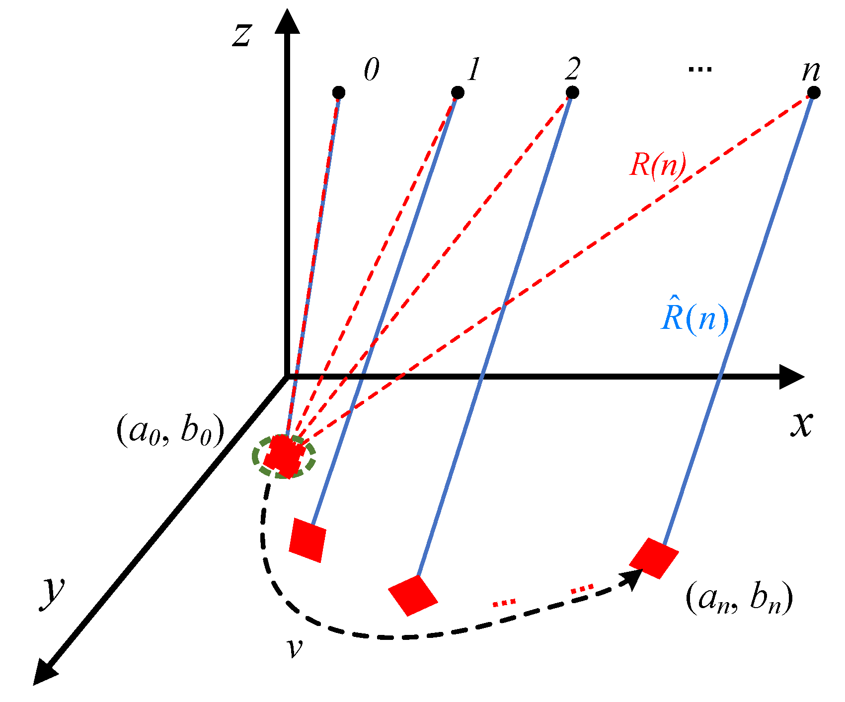
To analyze the signal characteristics of moving target, we model the geometry of an SAR system for observing a ground moving target as shown in Figure 1, in which x denotes azimuth direction, i.e., the direction that the platform moves, y and z denote range and height directions, respectively. The platform is at position $(x_n,y_n,z_n)$, where $n\in \left[-T/2,T/2\right]$ is slow time and T is data acquisition time.

The linear frequency modulated (LFM) signal emitted by the radar system can be expressed as:

$$s_t\left(t\right)=A{e}^{j2\pi f_{c}t}{e}^{j\pi K{t}^2},t\in [-T_p/2,T_p/2],$$

(1)

where A denotes the signal amplitude, $f_c$ represents the carrier frequency and K indicates the frequency sweep rate, t is fast time, and $T_p$ is pulse width of the LFM signal.

The corresponding received signal at different slow times can thus be expressed as:

$$s_r(t,n)=\sigma e^{-jk2\widehat{R}\left(n\right)}{e}^{j\pi K{(t-\tau )}^2},$$

(2)

in which the first term, $\sigma$, represents the target backscattering coefficient, the second term is the Doppler signal, and the third term denotes fast-time signal. n is slow time, $\tau$ represents target echo delay,

$$\tau =\frac{2\widehat{R}\left(n\right)}{c},$$

(3)

where c denotes speed of light and $\widehat{R}\left(n\right)$ is the slant range. Given that the moving target is at position $(a_n,b_n)$ at time n and the platform is at position $(x_n,y_n,z_n)$, Slant range of the moving target $\widehat{R}\left(n\right)$ is

$$\widehat{R}\left(n\right)=\sqrt{{(x_n-a_n)}^2+{(y_n-b_n)}^2+z_n^2}.$$

(4)

Ignoring range migration correction and only focusing on azimuth signal, we can write the moving target azimuth signal model as:

$$\widehat{s}\left(n\right)=e^{-jk2\widehat{R}\left(n\right)},$$

(5)

where $k=2\pi /\lambda$ represents wave number and $\lambda$ denotes signal wavelength.

2.2. Imaging Analysis

Typical SAR imaging algorithms include range Doppler (RD), chirp scaling (CS), back-projection (BP), etc. The imaging procedures of these algorithms can be considered as the process of matched filtering [38]. This section briefly reviews the features of moving targets in SAR images based on the BP algorithm.

The basic idea of BP is to calculate the distance between each pixel in the projection region and the SAR Antenna Phase Center (APC) in the aperture and coherently accumulate the echoes to reconstruct the scattering coefficient of each pixel, the procedures of which mainly consist of [38]:

(a) 

Range compression: range compression is implemented via pulse compression technique on the received SAR echoes at different times to achieve aggregation of scattering point energy along the range direction.

(b) 

Calculating echo delay: calculating echo delay from scattering point $\mathbf{p}$ to SAR at different times:

$$\tau =\frac{2R(n,\mathbf{p})}{c},$$

(6)

where $R(n,\mathbf{p})$ is

$$R(n,\mathbf{p})=\sqrt{{\left(x_n-u\right)}^2+{\left(y_n-v\right)}^2+{\left(z_n-w\right)}^2},$$

(7)

$(x_n,y_n,z_n)$ is the position of APC at time n, $u,v$ is the position of $\mathbf{p}$ and w is the projected height. The projection coordinate system is usually a Cartesian coordinate system and w is 0.

(c) 

Data interpolation/resampling in range: since the range compressed SAR data obtained in (a) is discrete and the echo delay calculated in (b) is continuous, to acquire echo at time $\tau$, interpolation is essential to the discrete SAR data after range compression and resampling is necessary at time $\tau$.

(d) 

Coherent accumulation: compensate the Doppler phase generated by the scattering point $(u,v)$ at different times and add the compensated data at different times to obtain the scattering coefficient of $(u,v)$. The signal with the compensated Doppler phase can be calculated by the following formula:

$$s\left(n\right)=e^{jk2R\left(n\right)},$$

(8)

where $R\left(n\right)$ is the slant range of stationary target.

For moving target, the azimuth signal after phase compensation using the standard SAR imaging algorithm can be obtained by Equations (5) and (8):

$$\begin{array}{cc}\hfill \Delta s\left(n\right)& =e^{jk2R\left(n\right)}{e}^{-jk2\widehat{R}\left(n\right)}\hfill \\ & =e^{-j2k\Delta R\left(n\right)}\hfill \end{array}$$

(9)

Due to the serious mismatch between the moving target signal and the reference signal of the stationary target, there exists offset and defocusing to the moving target in the SAR image.

$$\begin{array}{cc}\hfill \Delta R\left(n\right)& =\widehat{R}\left(n\right)-R\left(n\right)\hfill \\ \hfill & ={[{(x_n-a_n)}^2+{(y_n-b_n)}^2+z_n^2]}^{1/2}-{[{(x_n-a_0)}^2+{(y_n-b_0)}^2+z_n^2]}^{1/2}.\hfill \end{array}$$

(10)

Expanding Equation (10) with Taylor expansion, we can obtain:

$$\Delta R\left(n\right)=〈{\mathit{\alpha }}_n,\mathit{v}〉n+\frac{1}{\widehat{R}\left(n\right)}\left[〈\mathit{v},\mathit{v}〉-{\left(\frac{〈{\mathit{\alpha }}_n,\mathit{v}〉}{\widehat{R}\left(n\right)}\right)}^2\right]n^2,$$

(11)

where

$$\begin{array}{cc}\hfill {\mathit{\alpha }}_n& =\frac{[x_n-a_0,y_n-b_0,z_n]}{\widehat{R}\left(n\right)},\hfill \\ \hfill \mathit{v}& =[v_x,v_y,v_z],\hfill \end{array}$$

(12)

${\mathit{\alpha }}_n$ is the line of sight vector and $\mathit{v}$ is the velocity vector. $〈·,·〉$ represents inner product operation. While $\widehat{R}\left(n\right)\gg 1$, we can ignore $\frac{〈{\mathit{\alpha }}_n,\mathit{v}〉}{\widehat{R}\left(n\right)}$ term and Equation (11) can be simplified:

$$\Delta R\left(n\right)=〈{\mathit{\alpha }}_n,\mathit{v}〉n+\frac{{\parallel \mathit{v}\parallel }^2}{\widehat{R}\left(n\right)}{n}^2.$$

(13)

It can thus be obtained

$$\Delta s\left(n\right)=e^{-j2k\left(〈{\mathit{\alpha }}_n,\mathit{v}〉n+\frac{{\parallel \mathit{v}\parallel }^2}{\widehat{R}\left(n\right)}{n}^2\right)},$$

(14)

where the first term mainly causes distinct offset to moving target in SAR image and the second term leads to defocusing of moving targets. A lot of literature has quantitatively analyzed the offset and defocusing of moving targets [39,40,41,42,43].

2.2.1. Defocusing in Azimuth

Substitute Equation (11) to the radar azimuth echo formula and obtain:

$$\begin{array}{cc}\hfill \Delta s\left(n\right)& =e^{jk2R\left(n\right)}{e}^{-jk2\tilde{R}\left(n\right)}\hfill \\ & =e^{-j2k\Delta R\left(n\right)}\hfill \\ & =e^{-j2k\left(〈{\mathit{\alpha }}_n,\mathit{v}〉n+\frac{{\parallel \mathit{v}\parallel }^2}{\widehat{R}\left(n\right)}{n}^2\right)},\hfill \end{array}$$

(15)

in which $k=2\pi /\lambda$ is wave number and $\lambda$ is wavelength. The second term in this equation indicates azimuth defocusing. The bandwidth should be smaller than the azimuth resolution of the system. Assume azimuth sampling rate as PRF and accumulated points as Na. The azimuth frequency resolution (undersampling is not taken into consideration) is:

$$\begin{array}{c}T=Na/PRF,\hfill \\ \Delta f=1/T=PRF/Na.\hfill \end{array}$$

(16)

The frequency function is obtained by second-order phase derivation:

$$\frac{8\pi }{\lambda }\frac{{\parallel \mathit{v}\parallel }^2}{{\widehat{R}}_n}n=2\pi \left(\frac{4}{\lambda }\frac{{\parallel \mathit{v}\parallel }^2}{\widehat{R}\left(n\right)}\right)n.$$

(17)

The slope of sweep frequency signal is $\frac{4}{\lambda }\frac{{\parallel \mathit{v}\parallel }^2}{\widehat{R}\left(n\right)}$, and the bandwidth of the secondary signal is

$$B=\left(\frac{4}{\lambda }\frac{{\parallel \mathit{v}\parallel }^2}{\widehat{R}\left(n\right)}\right)T.$$

(18)

For example, suppose the target is moving at the speed of 5 m/s, the wavelength is 0.03 m, the range of action is 12 km, the synthetic aperture time is 5 s and PRF is 2000. The generated bandwidth by the moving target is thus 1.3889 and the azimuth frequency resolution is 0.2 Hz. Defocusing happens.

2.2.2. Offset in Azimuth

Azimuth offset is generated by the first order component

$$e^{-j\frac{4\pi }{\lambda }{v}_{r}n},$$

(19)

and its phase function is

$$4\pi \frac{v_r}{\lambda }n=2\pi \left(\frac{2v_r}{\lambda }\right)n.$$

(20)

The frequency offset generated by the moving target is

$$\frac{2v_r}{\lambda }\left(Hz\right).$$

(21)

In addition, calculate the physical distance of offset: under squint condition, distance history in the azimuth of the stationary target is $\widehat{R}\left(n\right)$ and expand it by Taylor expansion with respect to n, we have

$$\widehat{R}\left(n\right)=\widehat{R}\left(0\right)+\frac{v_p\Delta y}{R}n.$$

(22)

Modulating it on the echo signal, we have

$$e^{-j\frac{4\pi }{\lambda }\frac{v_p\Delta y}{R}n}.$$

(23)

Equaling Equations (19)–(23), we have

$$2\frac{v_r}{\lambda }=2\frac{v_p\Delta y}{\lambda R},$$

(24)

i.e., the offset of moving target is

$$\Delta y=\frac{v_{r}R}{v_p}.$$

(25)

For example, suppose the target radial velocity is 3 m/s, the range of action is 800 km and the platform speed is 7600 m/s. The target offset is thus 3 × 800 × 1000/7600 = 315.8 m.

From the above analysis we can observe that there exists severe offset and defocusing of the moving target in the SAR image. Offset and defocusing may lead to the moving target to be located outside the imaging region and increase the difficulty of moving target detection. In addition, in order to interpret a moving target, apart from detecting the moving target, refocusing is also needed.

3. Shadow Characteristics of Moving Target

The shadow is crucial to track a moving target on the ground, and we will discuss the influence of wavelength, angle of incidence, aperture time, target size and speed on the shadows in detail in this section. It should be noticed that the diffraction effect is ignored in our analysis because the target size is much larger than the wavelength.

3.1. Size of Shadow

Because of the shielding effect of the target, the scattering point on the ground cannot interact with the radar electromagnetic wave, which leads to shadowing.

For stationary targets, the SAR image is composed of the target and its shadow. When the target is moving (i.e., range and azimuth velocity are both not zero), its shadow will separate form its defocused image significantly due to the deviation phenomenon caused by the Doppler frequency, which makes the shadow easy to be detected.

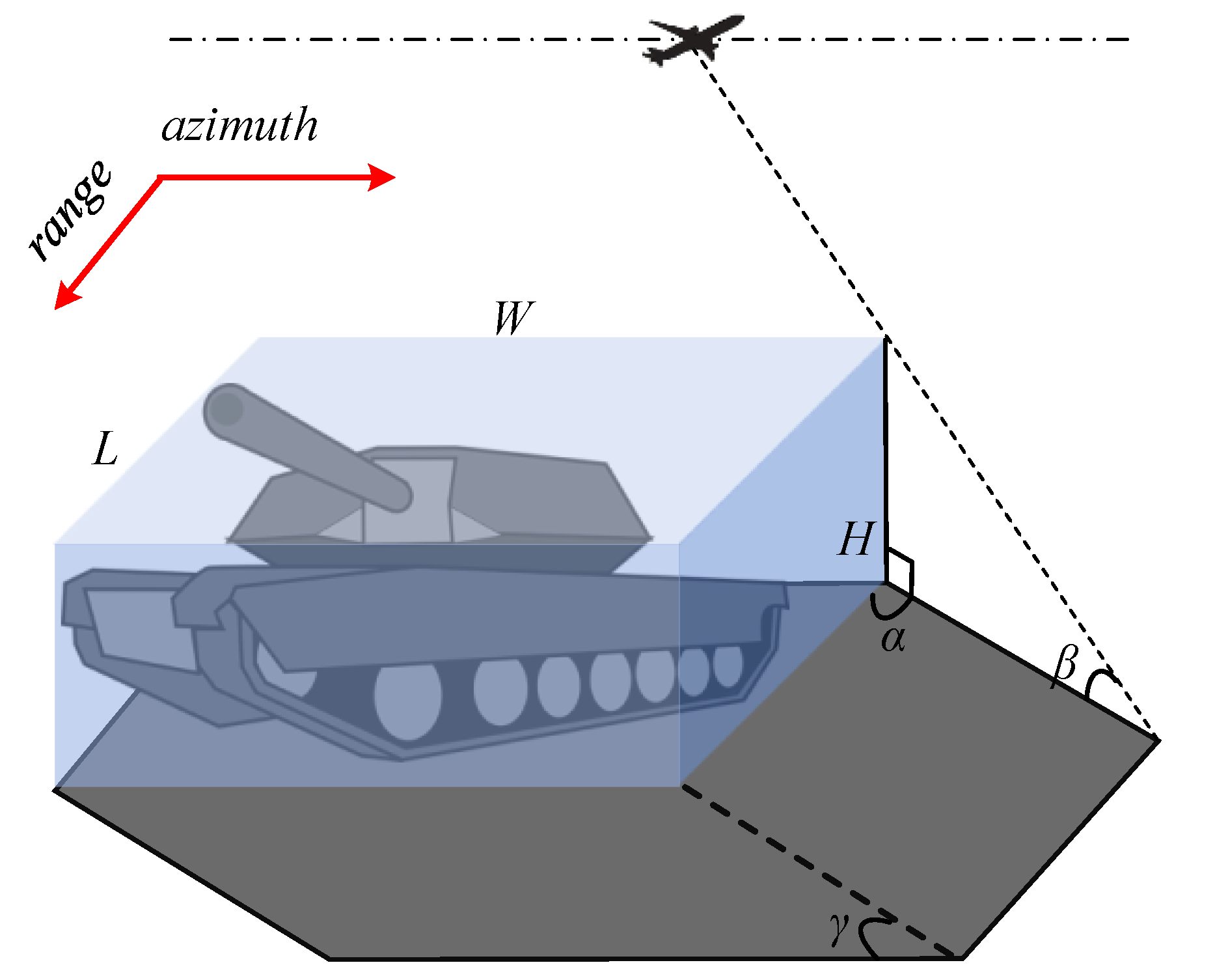
For moving targets, the shadow is composed of two components. One is the coverage area directly below the target and the other is the sheltered area, as shown in Figure 2, in which the azimuth and range direction is the same as the directions of the shadow’s length and width, respectively.

It can be observed from the figure that the width of the shadow can be computed by:

$$W_{\mathrm{shadow}}=W_{}+H_{}tan({90}^{\circ }-\beta )sin\alpha ,$$

(26)

where W and H denote the width and height of the target, respectively. $\beta$ is the pitch angle, $\alpha$ is the angle between the radar beam direction and the direction of target length. When the object can be modeled as a cube as illustrated in Figure 2, the length of the target is perpendicular to the azimuth direction, and the angle is the squint angle $\theta$. The length of the shadow of the target can be calculated by:

$$L_{\mathrm{shadow}}=L_{}+H_{}tan({90}^{\circ }-\beta )sin\gamma ,$$

(27)

where $L_{}$ is the length of target and $\gamma$ equals $({90}^{\circ }-\theta )$.

From the above analysis we can observe that the size of the target shadow is not only related to the size of target itself, it is also decided by the antennas pitch and squint angles. The larger the target width is and the taller the height is, the larger the shadow width is; the longer the target is and the larger the squint angle is, the longer the shadow is.

3.2. Effect of Shadow on Echo

Given a ground scattering point P sheltered by moving target, the sheltered time is decided by size and speed of target, i.e.,

$$T_{\mathrm{shadow}}=\frac{L_{\mathrm{target}}}{v_t},$$

(28)

where $v_t$ is the target velocity. $T_{\mathrm{shadow}}$ is the sheltered time and the synthetic aperture time of its corresponding scattering point is $T_{Aper}$. Given a point target, echo within a synthetic aperture time can be ideally expressed as:

$$s\left(n\right)=e^{jkR\left(n\right)},n\in \left[\frac{-T_{Aper}}{2},\frac{T_{Aper}}{2}\right].$$

(29)

When the target is above the shadow, the scattering point has partial echo sheltered in the synthetic aperture time and its echo is:

$$s\left(n\right)=U\left(n\right)e^{jkR\left(n\right)},n\in \left[\frac{-T_{Aper}}{2},\frac{T_{Aper}}{2}\right],$$

(30)

where

$$U\left(n\right)=\left\{\begin{array}{c}1,n\notin {\mathrm{T}}_{shadow},\hfill \\ 0,n\in {\mathrm{T}}_{shadaw}.\hfill \end{array}\right.$$

(31)

We can find that the generation of shadow needs the scattering point to be sheltered by the target within synthetic aperture time, i.e.,

$$T_{\mathrm{shadow}}\ge T_{\mathrm{Aper}}.$$

(32)

We define

$$T_{\mathrm{shadow}}=\kappa T_{\mathrm{Aper}},$$

(33)

where $\kappa$ is the shelter factor. To make the shadow significant, the synthetic aperture time should be less than or equal to the sheltered time, i.e., $\kappa \ge 1$. At this moment, the scattering point P is completely sheltered and the echo at this position is 0. When $\kappa \le 1$, the ground scatterers are partially sheltered, it can be considered as a sub-aperture imaging problem, and we have a dim and low-resolution image of these ground scatterers.

3.3. The Degradation of Shadow

Sheltered time is decided by target size and speed. Given a sheltered time, system parameters also have a significant influence on the shadow. When the size and speed of moving targets are fixed, $T_{shadow}$ is fixed. To ensure that all the sheltered areas in the imaging result are shaded, the maximum synthetic aperture time of SAR is $T_{shadow}$. The azimuth resolution of SAR is:

$${\rho }_{azi}=\frac{\lambda R}{2T_{Shadow}{v}_p},$$

(34)

where R is the distance from target to radar platform, $v_p$ is the velocity of radar platform.

3.3.1. Blur Due to Small Aperture

Assume the length of the moving target along the velocity direction is 5 m and the width is 2 m. The speed of the moving target is 5 m/s, the wavelength of SAR is 0.03 m, the distance from platform to target is 12 km and $v_p=100$ m/s. The synthetic aperture time is thus $T_{Aper}=1$ s. The azimuth resolution of SAR (side-looking) is 1.8 m. For a target with a length of $5$ m, the resolution of 1.8 m causes that the number of pixel of the shadow in the image is less than 3. Considering the sidelobe effect, the target is difficult to be detected from the image. When the system resolution increases to 0.2 m, the shadow occupies 50 pixels in the image, which is easy to be detected. In addition, since the resolution increases, the target locating accuracy improves, which further increases the speed accuracy of the system.

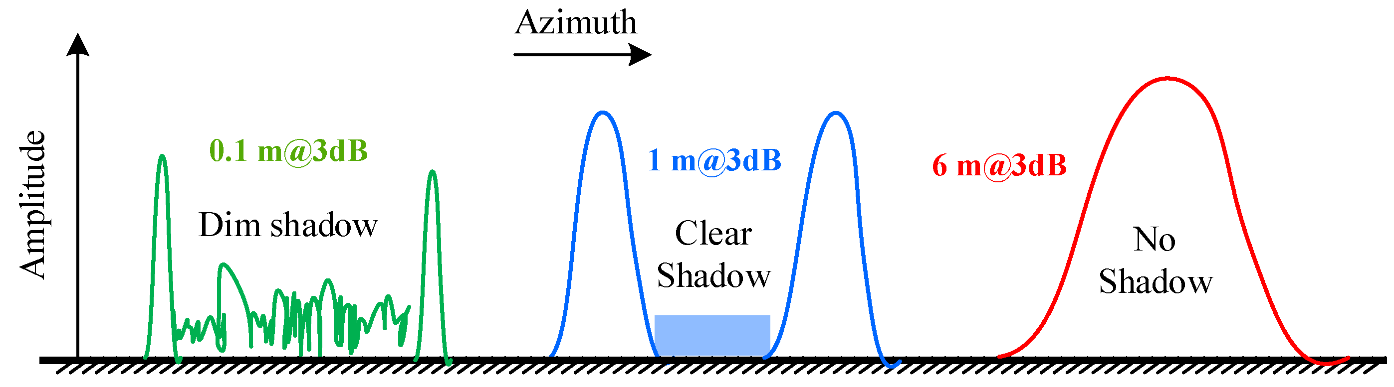
Generally, when the azimuth resolution is very low, the shadow of the target will always be submerged with the background noise, which makes it difficult to reconnoiter the shadow, as illustrated in Figure 3 (right). The increasing of the azimuth resolution improves the quality of the target shadow, which makes the shadow clear, as illustrated in Figure 3 (middle). However, when the azimuth resolution reaches a certain resolution, improving resolution does not help with further improving the imaging performance of shadow. The accumulated energy of the background in one pixel reduces with the increasing of the resolution, which reduces the contrast between shadow and background. As shown in Figure 3 (left), the shadow of the ground moving target may be dim when the resolution is high.

3.3.2. Fading Due to Large Aperture

For a target with the length $L_{target}$ of 6 m and width of 3 m, assuming that the target can be detected while it has 6 pixels, the resolution is 1 m/s. Suppose the system wavelength is 0.03 m, the platform speed $v_p$ is 300 m/s, the distance from the target to the platform is 12 km.

$${\rho }_{azi}=\lambda R/2L_{Aper}.$$

(35)

According to Equation (35), the synthetic aperture length $L_{Aper}$ is 180 m. The synthetic aperture time is:

$$T_{Aper}=L_{Aper}/v_p=0.6s.$$

(36)

The maximum detectable speed is:

$$v_{max}=L_{target}/T_{Aper}=10m/s.$$

(37)

If the target moves at the speed of 5 m/s, the shelter factor in (33) is $\kappa =10/5=2$ and the echo in the shadow area is 0.

If we continue to increase azimuth resolution by raising synthetic aperture, the azimuth resolution is 0.1 m/s while the aperture reaches 1800 m. The synthetic aperture time is 6 s at the moment and the maximum detectable speed is 1 m/s. If the target speed is still 5 m/s and shelter factor is $\kappa =1/5=0.2$, the echo in the shadow area includes background energy, which leads to target shadow degradation.

From the above analysis we can observe that to detect the moving target the system should be designed in the following manner: short wavelength, high-speed platform and close range, i.e., shorter time to achieve greater aperture and resolution. On the target side, the faster the target speed is, the shorter the aperture time should be; the larger the target size is, the larger the shadow is.

4. Methodology

Our proposed framework for tracking and refocusing the ground moving target in the SAR image can be regarded as three parts. First, a video-SAR back-projection (v-BP) algorithm is designed to obtain SAR videos. Then, we employ deep-learning-based tracking network SiamFc to track and locate the shadows of the ground moving target to reconstruct its trajectory. Finally, the candidate trajectory is applied to refocus the ground moving target using the moving target back-projection (m-BP) algorithm newly proposed in this paper.

4.1. Video-Sar Back-Projection

Different from traditional SAR imaging, video-SAR can obtain multi-frame images, which is helpful for surveillance tasks. Video-SAR algorithms root from the standard SAR imaging algorithms, such as back-projection algorithm [44,45,46] or polar format algorithm (PFA) [47]. Compared to the polar format algorithm, the back-projection-based algorithm projects the echoes to the same projection grid, i.e., automatic multi-frame registration, which is beneficial to tracking the shadow of moving targets. To this end, the video-SAR back-projection algorithm (v-BP) is designed to obtain automatic-registered SAR videos in this work.

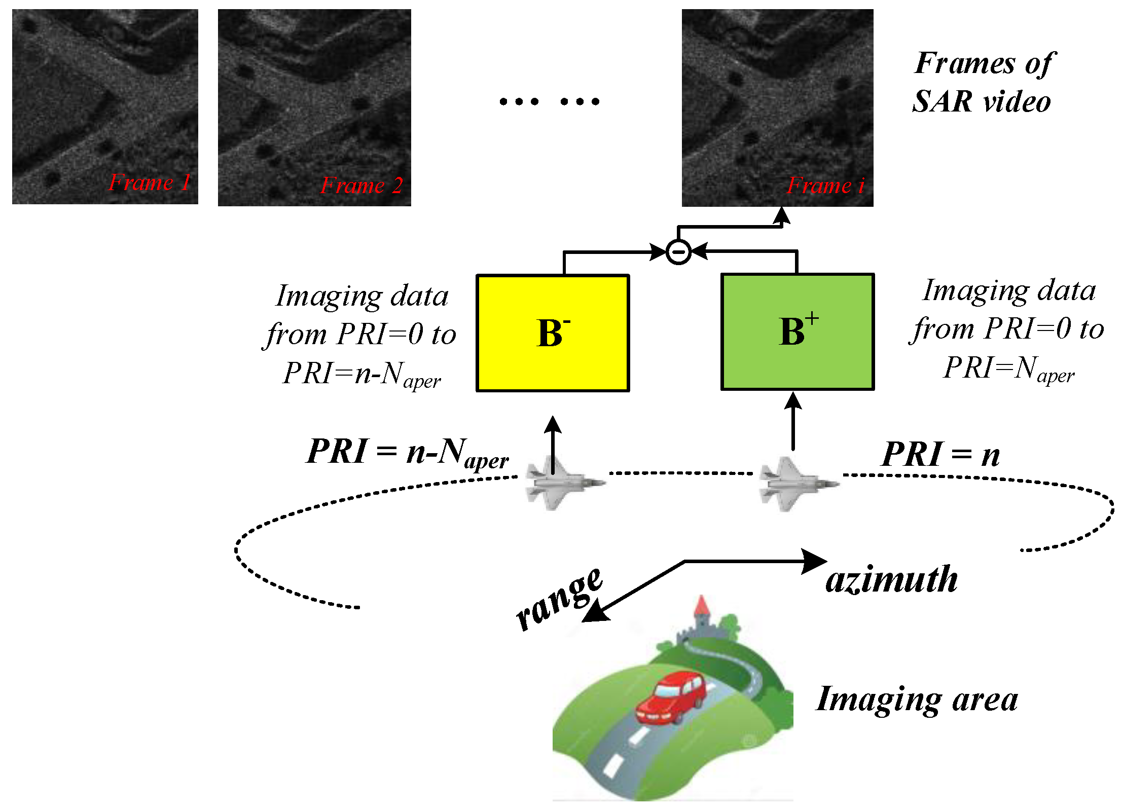
The diagram of the v-BP algorithm is illustrated in Figure 4. The transmitter radiates LFM pulses into the observation area with a fixed pulse repetition frequency (PRF), and the electromagnetic waves inspire the scattering electromagnetic fields that arrive at the receiver with some delays. The receiver acquires the echoes corresponding to the different pulse repetition indices (PRIs) after a specific delay, and arranges them into a 2-D array, which is known as the SAR raw data. $B^{+}$ and $B^{-}$ are two buffers that store the imaging results of the corresponding raw data from the first PRI to the n-th PRI and the first PRI to the $(n-N_{aper})$-th PRI, respectively, in which $N_{aper}$ is the number of PRIs contained in every synthetic aperture time of video-SAR. Each frame of the video-SAR can be obtained by subtracting $B^{-}$ with $B^{+}$.

More details about the v-BP are shown in Algorithm 1, in which $P(·)$ represents the standard BP imaging processing module that includes range compression, calculating echo delay, data resampling and coherent accumulation. f denotes frame interval, i.e., the number of f PRI data is added to the current frame from the previous frame. The number of f and $N_{aper}$ can be adjusted arbitrarily in our video-SAR imaging algorithm.

As shown in algorithm 1, raw data is fed into $P(·)$ in the form of a data stream to perform imaging processing and is stored in the $B^{+}$ buffer. When the number of PRI reaches $N_{aper}$, the imaging result is read from $B^{+}$ buffer and used as initial frame $F\left(0\right)$ in video-SAR. Meanwhile, the data in $B^{+}$ buffer is imposed on $B^{-}$ buffer. A new frame $F\left(i\right)$ is obtained by $B^{+}-B^{-}$ after each newly-processed the number of f PRI raw data by BP module $P(·)$, until all the data is processed.

With this method, repeated processing of multiplexed data segments can be avoided to further improve the efficiency of multi-frame imaging and achieve real-time high frame rate monitoring. Furthermore, due to its fixed projection grid, the shadow motion has a clear geometric meaning, which is convenient for estimating the position and velocity of moving targets and provides necessary information for moving target focusing.

Algorithm 1 Video-SAR back-projection algorithm.

Ensure:  $B^{+}=0$;  $B^{-}=0$;  $i=0$;  for n in all PRIs do   $B^{+}=B^{+}+P\left(n\right)$;   if $mod(n,f)==0$ then    if $n==N_{aper}$ then     $F\left(i\right)=B^{+}$;     $B^{-}=B^{+}$;     $i=i+1$;    end if    if  $n>N_{aper}$ then     $F\left(i\right)=B^{+}-B^{-}$;     $B^{-}=B^{+}$;     $i=i+1$;    end if   end if  end if

4.2. Tracking Via Shadow

With the knowledge provided in the last section, a sound SAR system (typically in the spotlight mode) can be designed and a SAR video with vivid shadows for multiple targets via v-BP can be obtained. Then, tracking algorithm should be adopted to estimate the trajectories of moving targets. There are many algorithms for tracking task, including traditional correlation filter based methods [48,49] and deep learning based methods [50,51,52].

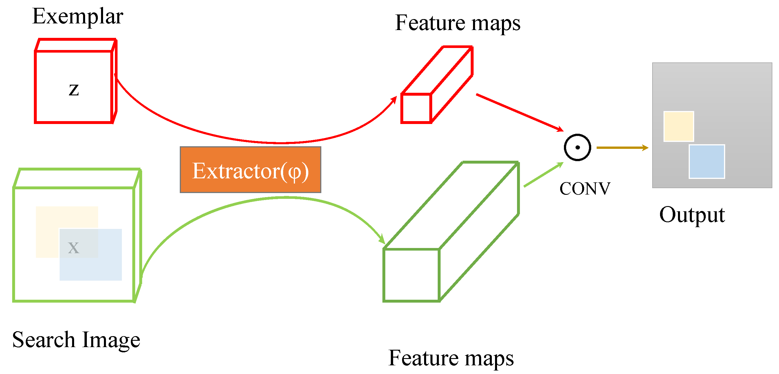
In this work, a deep learning tracking method, fully-convolutional Siamese network (SiamFc) [50] is employed to track shadows. SiamFc is a tracking network based on the feature similarity, it is also an extremely simple tracker that has the advantages of high precision, high speed, etc. It has widely been used in many computer vision tasks and obtained state-of-the-art tracking results. The network architecture of SiamFc is shown in Figure 5.

SiamFc has two branches with two inputs, z and x. Specifically, z is the exemplar image, i.e., the object to be tracked, and x is the much larger search image. SiamFc learns a function $f(z;x)$ that compares z to x and returns a high score if the two images depict the same object and a low score otherwise. The output of SiamFc is a scalar-valued score map, the dimension of which depends on the size of the search image x. Simply speaking, the network aims to locate z in x. To achieve this, a convolutional embedding function $\phi$, working as a feature extractor, is applied to both inputs. Combining the results of feature maps with a cross-correlation layer, we have

$$f(z;x)=\phi \left(z\right)\ast \phi \left(x\right)+b_1,$$

(38)

where $b_1$ denotes the value at each position of the score map and ∗ is the convolution operator. The convolution operation works to extract the part of x that is most similar to z. During tracking, the score map is calculated from the search image centered on the target position of the previous frame. The current location of the target can be obtained by multiplying the position of the maximum score with the stride of the network.

4.3. Moving Target Back-Projection

According to the analysis in Section II, the exist of $\Delta s\left(n\right)$ in (9) caused by $\Delta R\left(n\right)$ leads to offset and defocusing of the moving target in the SAR image [39,40,41,42,43], and the reference signal in (8) needs to be modified as the form of Equation (5) to refocus the moving target. Thus, we have

$$\Delta s\left(n\right)=e^{jk2\widehat{R}\left(n\right)}{e}^{-jk2R\left(n\right)}\equiv 1.$$

(39)

Therefore, to achieve accurate imaging of moving targets, the precise instantaneous positions within synthetic aperture time are necessary, which is estimated by utilizing the shadows of moving targets in this paper. With the instantaneous positions, a moving target back-projection (m-BP) algorithm is then applied for imaging of a moving target.

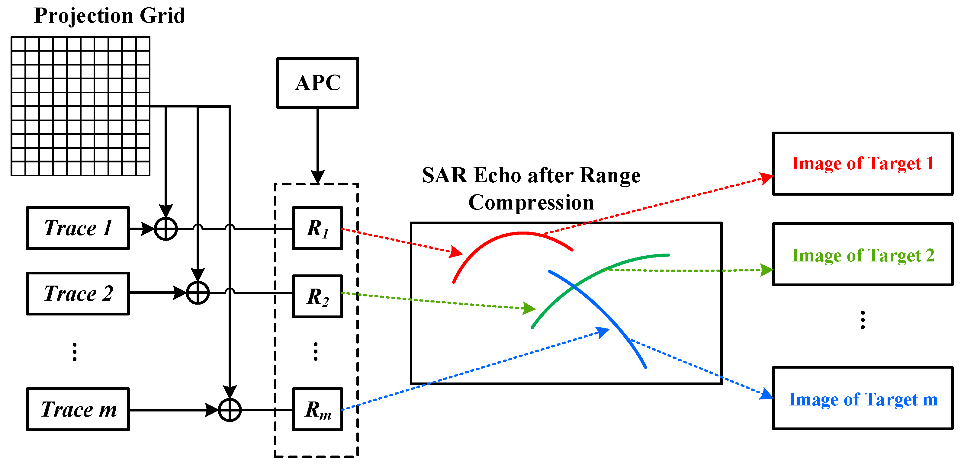
The flow chart of the m-BP proposed in this paper is shown in Figure 6, where m denotes the number of moving targets in the scene. Trace 1, Trace 2 and Trace m are the trajectories obtained by shadow tracking of the targets during imaging. A projection grid is the projection space of BP imaging, and APC denotes the antenna phase center.

To achieve imaging of moving targets, the projection grid of m-BP takes the moving target as the reference. When calculating the instantaneous distance, the coordinate of a pixel with respect to the original point of moving target is added to the current position of the original point. The grid position at the current moment is obtained, and the instantaneous distance of the grid point is from the grid position to APC as shown in Equation (4). If there are multiple targets, the distance history of each target needs to be calculated by using its respective trajectory, and m-BP needs to be called separately for imaging.

5. Experiment and Analysis

Our experiment was developed on CUDA C and the hardware platform was Intel i7-8700 CPU, NVIDIA GTX1080 GPU. To analyze effects of SAR platform parameters, such as height, speed, bandwidth and frequency, on tracking and refocusing results, we have carried out many simulation experiments. The SAR system works on spotlight mode to achieve continuous observation of the same area and obtain video-SAR data of this area.

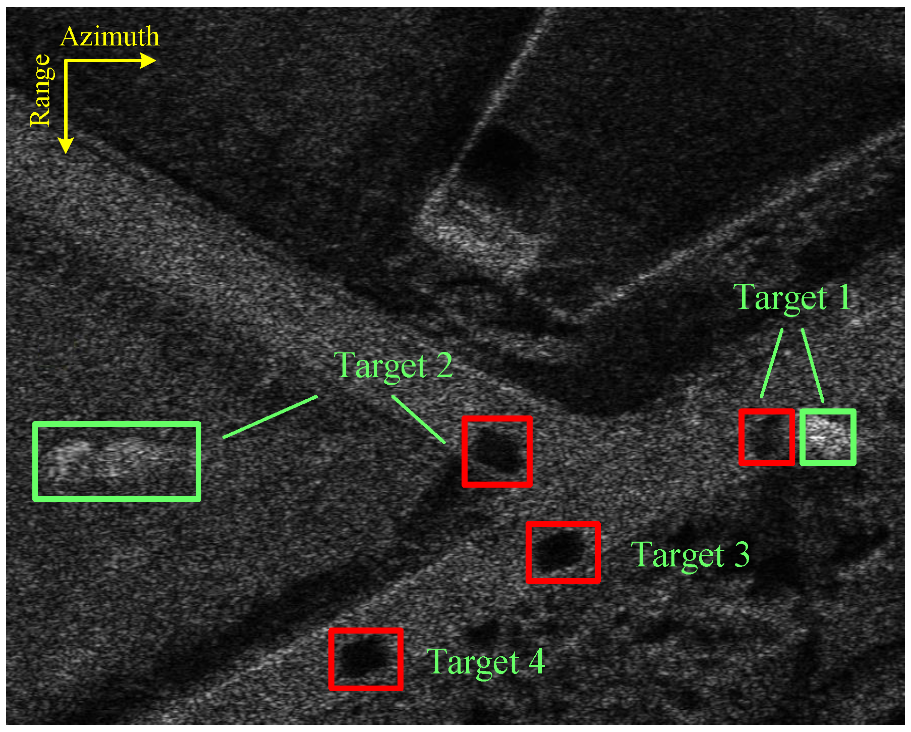
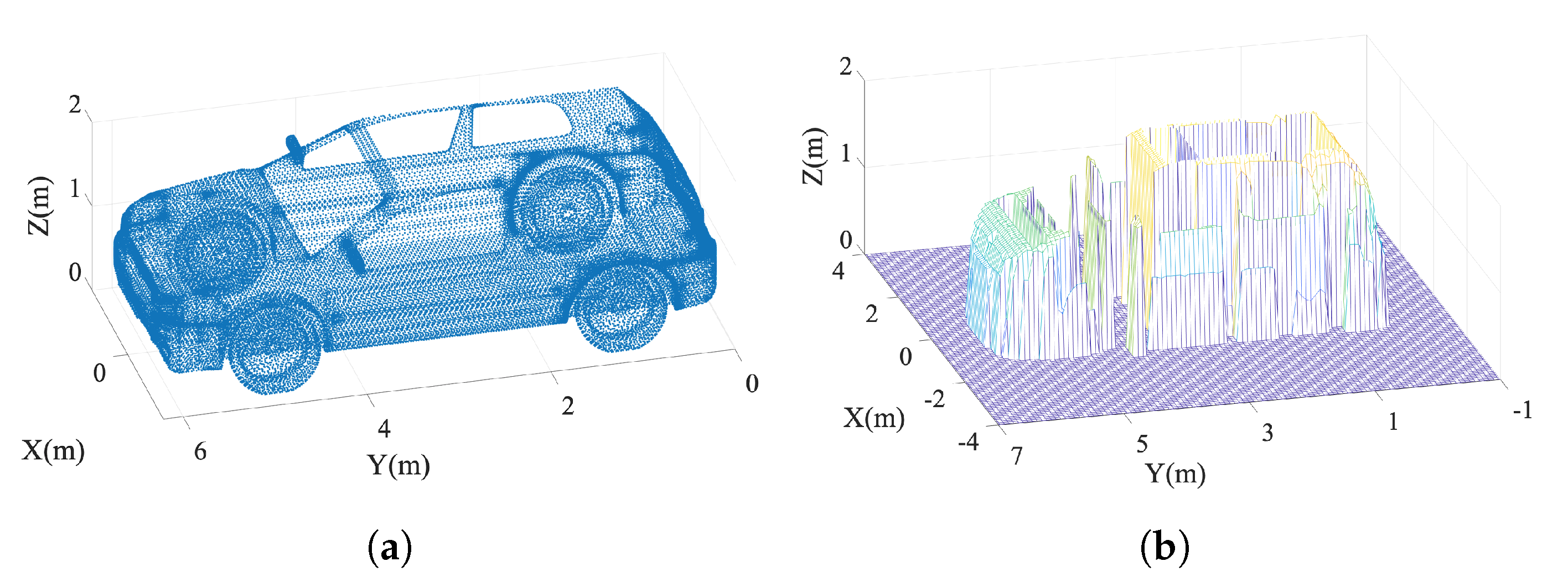
As shown in Figure 7, roads and vehicles are considered as background and moving targets, respectively. We applied FEKO [53] to construct scattering amplitudes of moving targets and implement target modeling. Since the problems of convergence, mesh size and frequency sweep analysis are independent of SAR simulation, surface current can be used as scattering characteristics. A geometric model of the moving target and a scattering coefficient model are illustrated in Figure 8. Simulation results of multiple moving targets with different speeds are shown in Figure 7, where shadows are marked with red rectangles and targets are marked with green rectangles. Azimuth speeds of these four targets are 0.5, 1.4, 3 and 3 m/s, respectively. Range speeds are the same as azimuth speeds. From the figure we can observe that, the larger the range speed is, the greater the target offset is. The larger the azimuth speed is, the more serious the target defocusing is.

When the speed is $(3\times 3)$ m/s, the moving target is completely off the road and cannot be located according to the imaging position directly. No matter how the target speed varies, its shadow position is fixed relative to the road, and it can thus be applied to locate tracking.

5.1. Shadow Feature

From the previous analysis we can find that moving target cannot be focused in the imaging result and offset also exists. However, the location of the shadow is fixed, which is conducive to interpreting the characteristics of the moving target. In this section, we analyze the influence of emission electromagnetic wave wavelength, radar platform speed, platform height, target speed and other factors on moving target shadow by modifying imaging parameters of simulation software. During simulation, we applied a fixed grid (0.1 m) imaging.

5.1.1. Effect of System Parameters on Shadow

Simulation parameters are as follows: imaging resolution is 0.1 m; PRF is 2000 Hz; platform speed is 330 m/s; platform height is 10 km; squint angle is ${45}^{\circ }$; bandwidth is 2 Ghz; SNR is 40 dB.

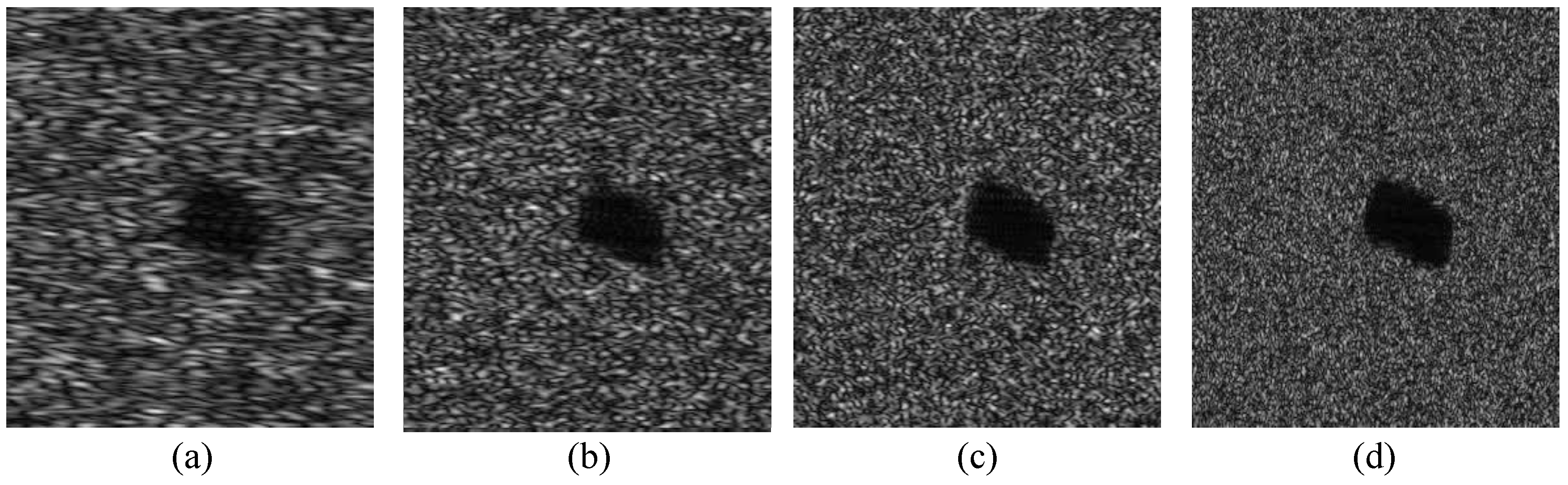
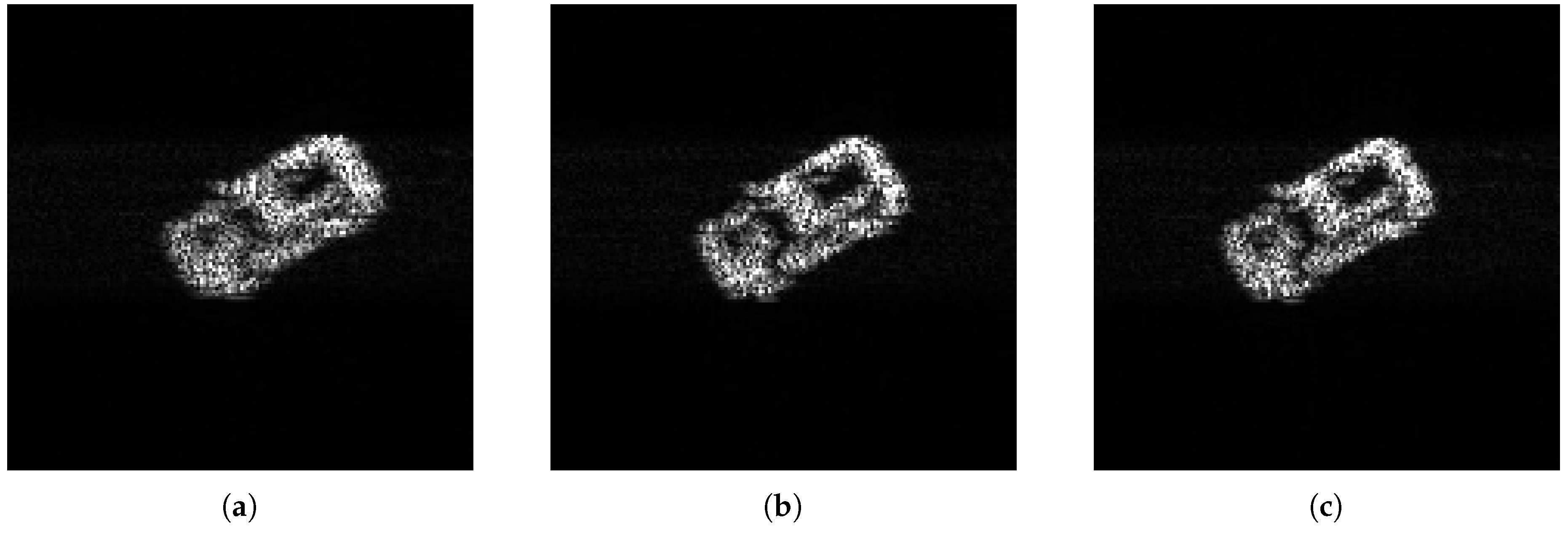
Figure 9 gives simulation results with different emission frequencies. From the figure we can observe that when the frequency is 5 GHz, the imaging effect of the shadow is poor, almost submerged by the surrounding environment. When the carrier frequency is 10 GHz, the clarity of the target shadow contour is significantly improved and when the carrier frequency increases to 16 GHz, the difference between the shadow edge and background is very obvious.

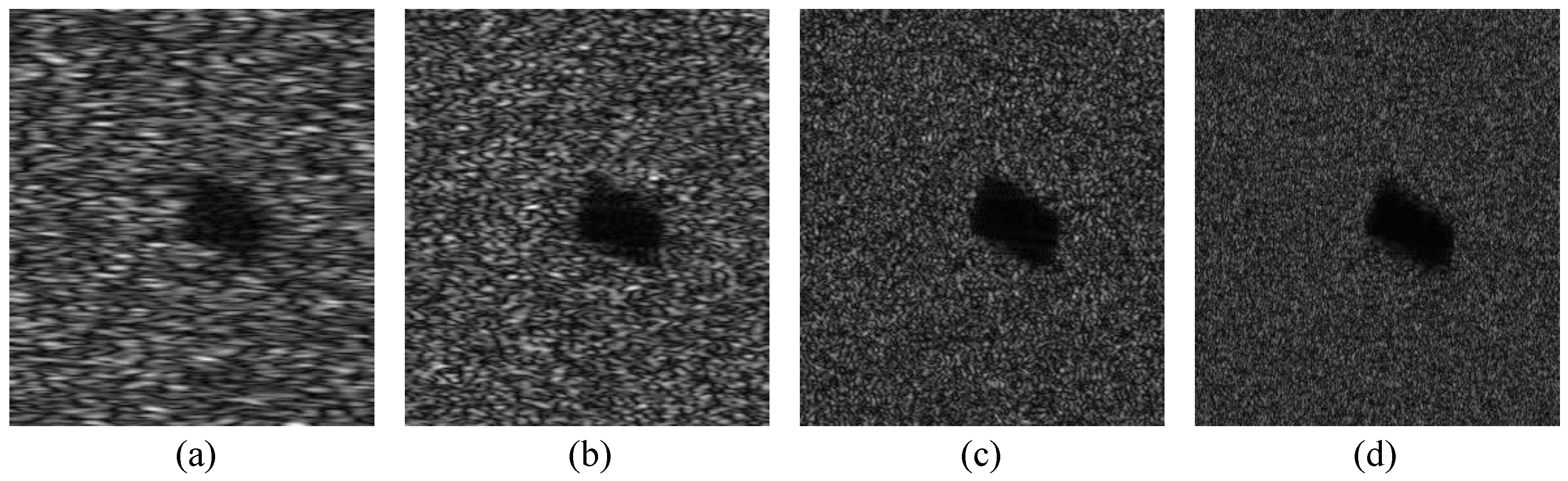
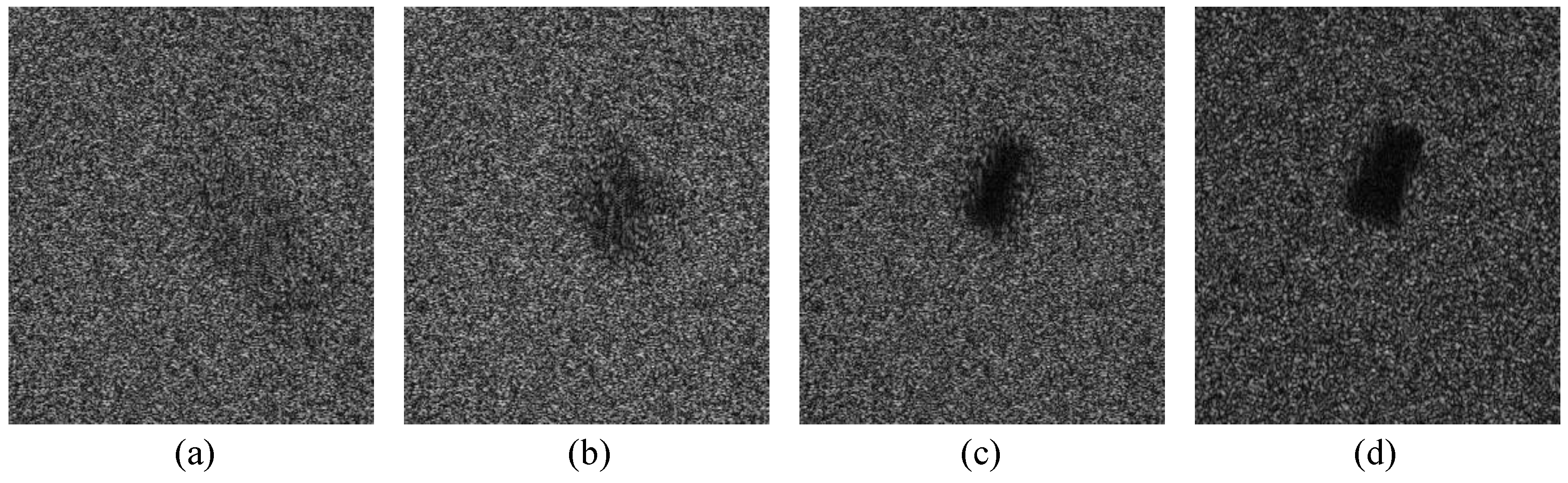
In addition, similar to the influence of frequency, with the increasing of synthetic aperture, the system resolution gradually increases, and the shadow of the target becomes clearer in the imaging result, as illustrated in Figure 10. Furthermore, the imaging result of the shadow is also affected by synthetic aperture time when the size of the aperture is fixed. As shown in Figure 11, for the target with speed of $(5\times 5)$ m/s, the shadow barely exists in the imaging result when the synthetic aperture time is 2 s. The shadow starts to exist in the imaging result but still without shape and contour information when the synthetic aperture time reduces to 1 s. The contour of the target shadow appears in the imaging result but with blurry edges when the synthetic aperture time continues decreasing to 0.5 s, and a clear shadow shows up in the imaging result when the synthetic aperture time is 0.3 s.

Overall, as the frequency increases, the wavelength decreases, the system resolution also increases, and the shadow of the target becomes clearer. Meanwhile, the increasing of synthetic aperture also makes the resolution of the system higher, and the shadow of the moving target thus becomes clearer. When the synthetic aperture time is relatively short, the ground scattering point corresponding to the shadow can be blocked by the target all the time during imaging and a clearer shadow can thus be obtained.

5.1.2. Effect of Target Parameters on Shadow

Simulation parameters are as follows: imaging resolution is 0.1 m; frequency is 35 GHz; PRF is 2000 Hz; platform speed is 330 m/s; platform height is 10 km; squint angle is ${45}^{\circ }$; bandwidth is 2 GHz; SNR is 40 dB.

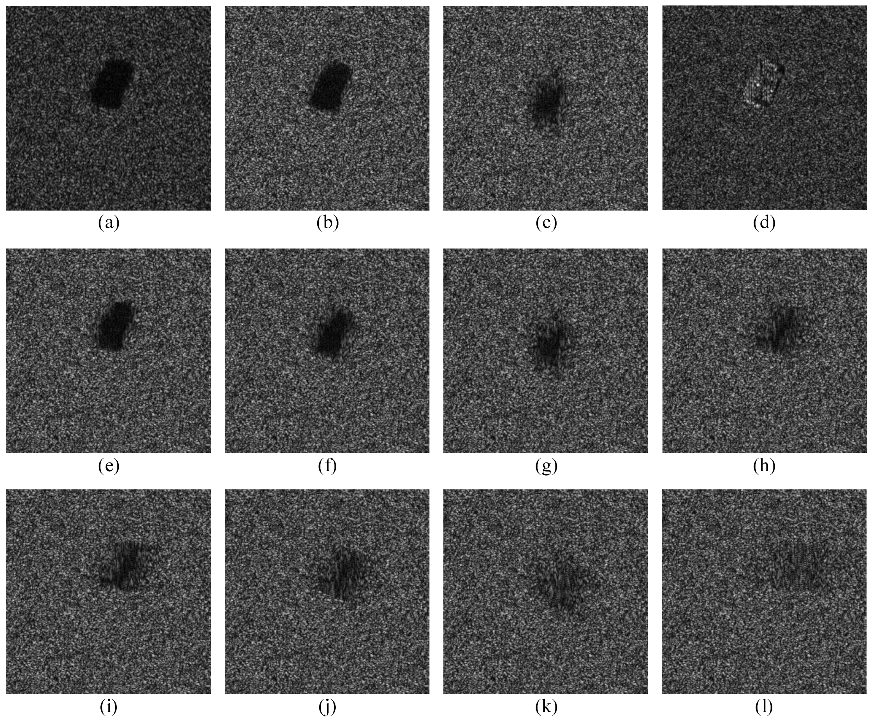
The simulation result is shown in Figure 12. From the figure we can observe that when the target azimuth speed is 0 and range speed is 1 m/s, the shadow can be prominently displayed in the imaging result. When range speed increases to 2 m/s, the shadow blurs at the edge of range, but the main body remains essentially contoured. When azimuth speed increases to 5 m/s, even though the target shadow can be seen in the imaging result, its edge shape and information of the subject are lost. It is thus impossible to distinguish the attributes.

From (d) we can find that, when range speed is 0, target imaging result is defocused, but there barely exists an offset. So that the shadow directly below the target in the imaging result is blocked by the target itself, and only a small area of the shadow is presented in the imaging result.

From the first row of the figure we can find that, when range speed is not 0, the shadow contours gradually blur (especially in the azimuth direction) as azimuth speed increases. Comparing (c) with (h) in the figure we can observe that, the increasing of range and azimuth speeds aggravate the fuzziness of the shadow in that direction. When the speed is high, the target shadow is mainly submerged in the clutter background as shown in (k) and (l).

Overall, offset will not exist in the imaging result when target radial velocity is 0 and available shadow can not be obtained. Offset happens in the target imaging result when radial velocity is not 0 and shadow appears at the actual position of target. When the target speed is small, the shadow contour is clear and the shape is complete. As the speed of the target increases, the shadow edge becomes blurred. When the speed is high, the shadow is completely submerged in the imaging scene.

5.2. Shadow Tracking

To validate the effectiveness of SiamFc on shadow tracking, we compare our method with two state-of-the-art traditional tracking methods, Minimum Output Sum of Squared Error (MOSSE) [48] and kernelized correlation filter (KCF) [49], and a learning based tracking method real-time recurrent regression network (Re${}^3$) [54]. Accuracy, robustness, and center distance error [55] are considered as evaluation metrics for tracking.

During simulation, to obtain high quality moving target shadow video, we have sacrificed the SAR azimuth resolution of the video to a certain extent, and its theoretical resolution is less than 0.5 m. Each aperture contains 2000 PRI data, the number of PRI between frames is 640, and the video frame rate is 1, which can be adjusted later as demanded.

Ten sets of simulated video data are used for training of the SiamFc network, while five sets of data are used for testing. Each set of videos consists of 60 images with a size of $1024\times 1024$. Network parameters are initialized by Gaussian distribution and gradient descent is adopted to train 2000 epochs with batch size of four. More information about the simulation data is shown in

Table 1. Details about the simulated data used for testing the algorithms.

Imaging Resolution	Carrier Frequency	PRF	Platform Speed	Platform Height
0.125 m	35 GHz	2000 Hz	330 m/s	10 km
squint angle	bandwidth	image size	FPS	PRI interval
45${}^{\circ }$	2GH	1024 × 1024	1	640

. The learning rate is annealed geometrically at each epoch from $0.01$ to $0.0005$. Figure 13, Figure 14, Figure 15 and Figure 16 give the tracking results of partial frames of SAR data in the same video with MOSSE, KCF, Re${}^3$ and SiamFc, respectively.

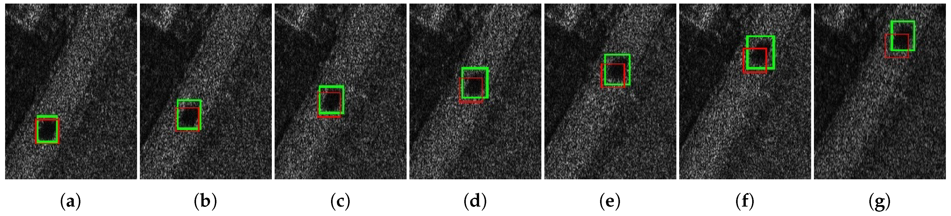
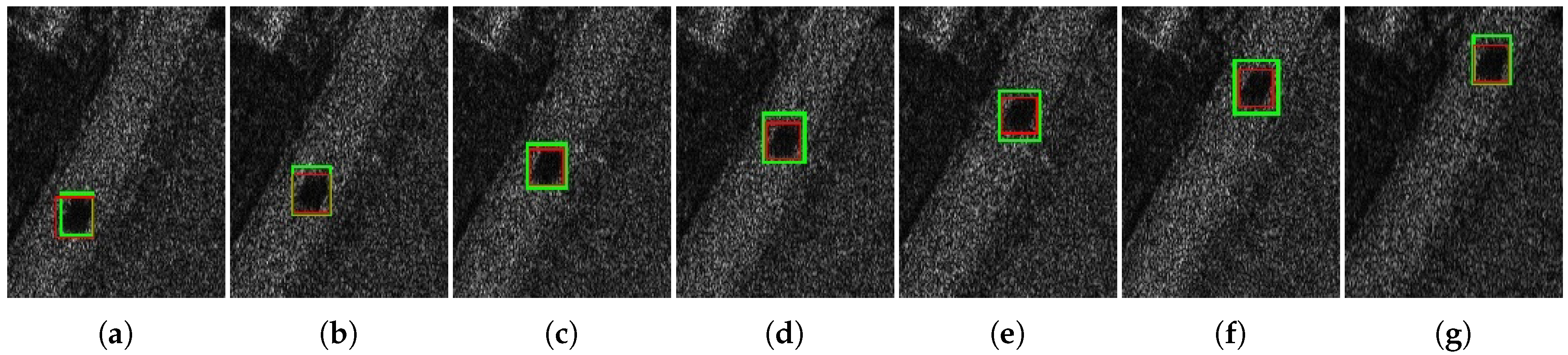
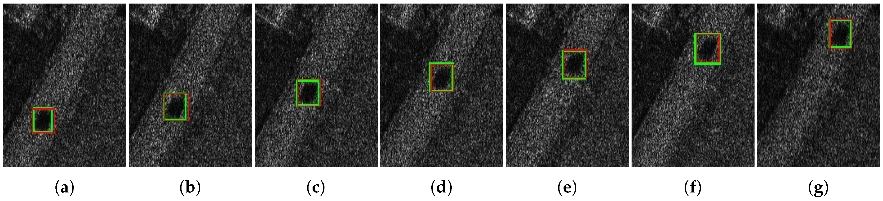
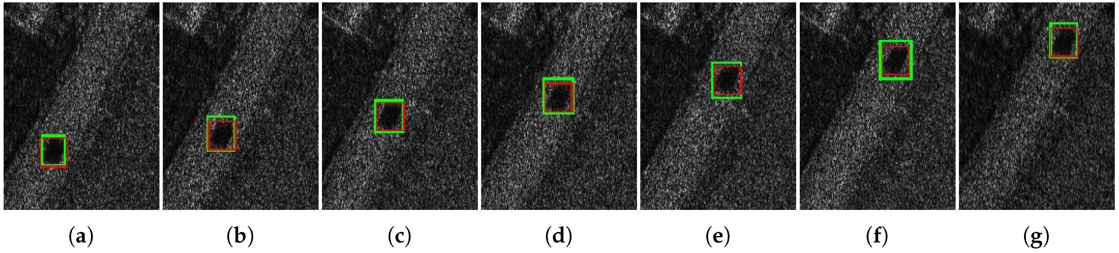
We can observe that these three algorithms can all realize continuously tracking of the shadow of a moving target, but with different performance. When the initial frame is at frame 0, the prediction box of MOSSE at the first frame is basically the same as ground truth. However, as time goes by, the tracking effect gradually gets worse, and the prediction box is offset from the ground truth. At frame 60, the coincidence rate of the two is very low, and the prediction box only covers part of the shadow. KCF and SiamFc perform much better than MOSSE, the tracking results of these two are not affected by the shifts of shadow. Nevertheless, we can also find that, SiamFc performs better than KCF since the prediction boxes of SiamFc are closer to the ground truths.

The comparison results of these three methods with all testing sets are shown in

Table 2. Tracking results with different methods on the simulated SAR dataset.

Index	Accuracy	Robustness	Distance
MOSSE	0.506	0.81	17.26
KCF	0.721	1.00	6.25
Re${}^3$	0.764	0.98	6.01
SiamFc	0.739	1.00	6.13

. From Table 2 we can observe that the tracking performance of MOSSE is not ideal, the center distance error of which reaches $16.33$. It indicates that the tracking result of MOSSE deviates greatly from the true position of the target, which is consistent with Figure 13. KCF achieves comparably good tracking result, accuracy, robustness, and center distance error of which are $0.701$, 1, and $7.28$, respectively. However, its accuracy is $0.039$ lower than SiamFc and center distance error is $1.24$ higher than SiamFc.

As a correlation filter-based tracking algorithm, MOSSE directly uses the appearance (pixels) feature of images to produce correlation peaks for each interested target in the scene while yielding low responses to the background. To obtain better performance, multi-channel HOG [56] feature is applied in KCF [57]. Furthermore, the SiamFc employs CNN to extract features of interested targets, which is extremely effective compared with a HOG feature and appearance (pixels) feature. Therefore, the SiamFc network has better tracking performance on the shadow of a moving target compared with traditional algorithms MOSSE and KCF.

Although Re${}^3$ has a slightly better accuracy and center distance error, its robustness is worse than SiamFc. More importantly, Re3 has a more complex structure than SiamFc and many tedious training tricks cannot be neglected to obtain a good tracking performance.

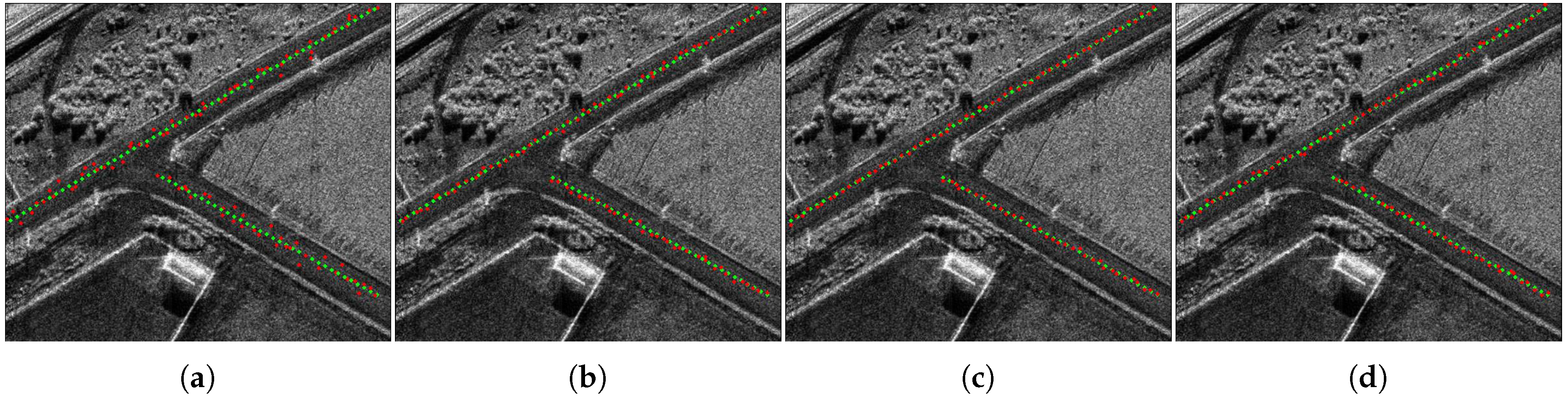
In addition, we reconstruct the trajectory of a moving target based on the tracking result as illustrated in Figure 17. The green dots denote the true positions of the simulated target and the red dots represent the centers of prediction boxes during tracking. Consistent with the previous analysis, the tracking results of SiamFc and KCF are closer to the true positions of the target, while the tracking results of MOSSE show a larger deviation.

5.3. Moving Target Refocusing

In this section, we first provide the effects of radar carrier frequency and target speed on moving target refocusing without estimation error. Then, we give the refocusing result based on the estimated trajectory. The influence of estimation error on refocusing is ultimately analyzed. The simulation parameters for moving targets are as follows: imaging resolution is 0.1 m; platform speed is 330 m/s; squint angle is ${45}^{\circ }$; bandwidth is 2 GHz; SNR is 40 dB.

5.3.1. Refocusing Analysis of Moving Target in Precise Compensation

Refocusing results of moving targets with different carrier frequencies and different target speeds are illustrated in Figure 18 and Figure 19.

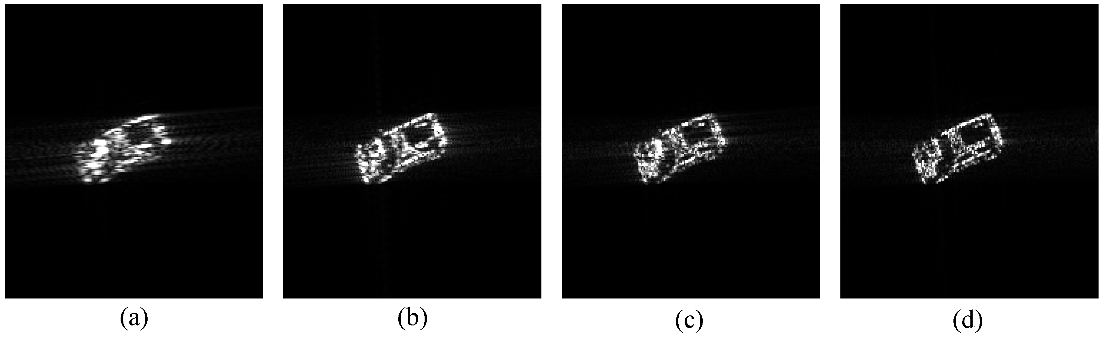
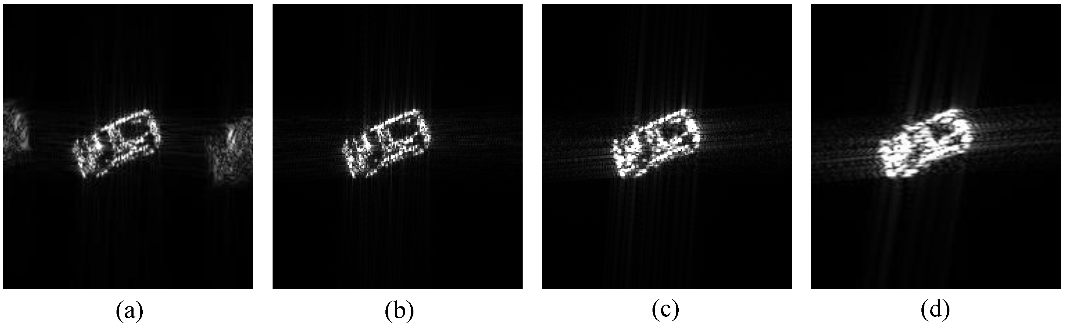
By comparison we can find that, the higher the frequency is, the shorter the wavelength is, the higher the system resolution is and the better the moving target refocusing is. When the carrier frequency is 5 GHz, the main contour of the target can be presented. The higher the carrier frequency is, the more obvious the target contour information is. When the carrier frequency is 35 GHz, the imaging result is able to present the detailed features of the moving target. Furthermore, as shown in Figure 19, when the system resolution is fixed, the increasing of the target speed causes a worse effect of refocusing. When the speed is $(1\times 1)$ m/s, the target detail features are significant and the refocusing effect is good. When the speed is $(5\times 5)$ m/s, the moving target can be refocused, but the resolution is significantly reduced.

5.3.2. Refocusing of Moving Target Based on Tracking Results

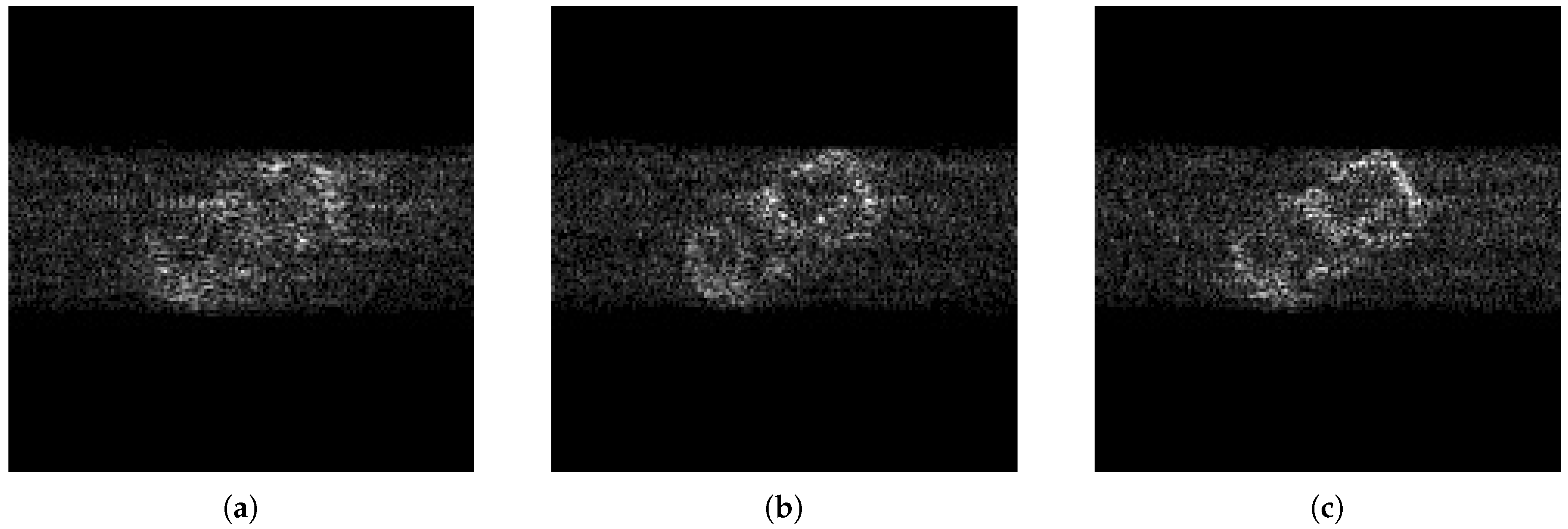
Refocusing results based on estimated trajectories of these three tracking methods are shown in Figure 20. The range and azimuth speeds of the target are both 5 m/s and imaging resolution is 0.1 m. We can observe that since the refocusing algorithm is sensitive to trajectory accuracy, there exists obvious defocusing phenomenon in the refocusing result by directly applying an estimated trajectory. However, SiamFc has higher estimation accuracy, and its moving target imaging result is relatively better. The geometric characteristics of the target can be basically observed. MOSSE on the contrary has low positioning accuracy of the target and a poor refocusing result, which makes it difficult to distinguish target contour information.

On the other hand, since this paper only discusses the case of uniform linear motion, the target trajectory can be smoothed by linear fitting. The refocusing result of moving target using linear smoothed trajectory is shown in Figure 21. It can be seen that after smoothing, the three methods all perform well in refocusing, and the difference in performance is also small.

It can be seen from the above analysis that for linear motion, due to its simple and regular motion, most trajectory estimation error can be eliminated by smoothing technology, and the accuracy required for shadow tracking is low. However, the ground target always performs non-uniform linear motion. At this time, the smoothing order is high, and the trajectory estimation error may not be completely eliminated. Therefore, for general moving targets, a high-precision trajectory estimation method is necessary.

5.3.3. Effect of Motion Parameters on Refocusing

When the target moves linearly with a uniform speed, only the target speed needs to be estimated to reconstruct the target trajectory and refocus image. In this section, by adjusting the actual speed of the moving target and the estimated speed during refocusing, we analyze the effect of speed error on refocusing.

As analyzed previously, azimuth speed leads to target offset in the imaging result. In the same way, the estimation error of range speed leads to deviation of the azimuth position of the target when the target is refocused.

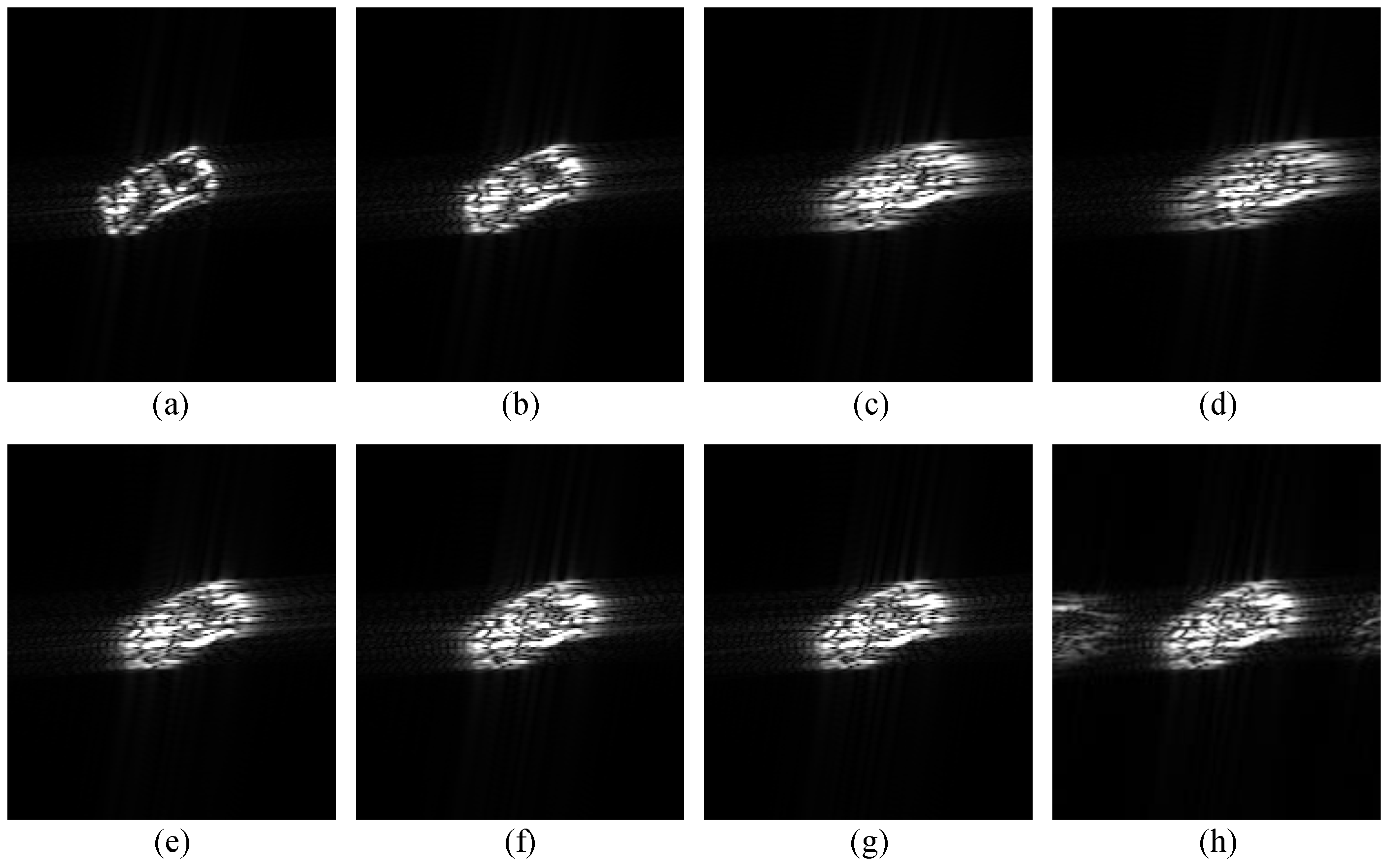
a∼e in Figure 22 give different azimuth speed errors when speed is $(10\times 10)$ m/s. The corresponding target speeds of f∼h are $(10\times 5)$ m/s, $(10\times 2)$ m/s and $(10\times 1)$ m/s. It can be found that when speed error is less than 0.5 m/s, the existence of error causes the target to be unable to be fully focused, resulting in blurry imaging results. However, the basic shape and scattering properties of the target can still be preserved, which provide the basis for detection and identification of further targets. When the estimated speed error continues to increase, target defocusing after image refocusing is serious, the shape and electromagnetic scattering characteristics of the target mainly disappear. Meanwhile, from e∼h in the figure we can observe that, when range speed is fixed, the focusing result is only related to the absolute speed error. The azimuth speed is different, but the absolute error is the same, the focusing result is still the same.

6. Discussion

Runtime is one significant evaluation index to measure the efficiency and feasibility of algorithms. This section will give the statistics of the run time of different parts of our refocusing framework based on the Intel i7-8700 CPU, NVIDIA GTX1080 GPU hardware platform.

For video-SAR, when the size of the image is $1024\times 1024$ and the frame interval is 320 PRI, the imaging time per frame is 0.6655 s, and when the video-SAR frame interval is 640 PRI, the imaging time per frame is 1.1438 s. For SiamFc, the tracking time of each frame is less than 0.01 s for a single target. m-BP has the same efficiency as the standard BP. When the aperture size is 20,000 PRI and the number of sampling points in the range is 20,000, the focusing time of the moving target is about 32 s.

It can be observed from the analysis above, video-SAR imaging and tracking steps basically satisfy the real-time processing, especially the SiamFc, which can track shadows with the speed of 100 frames per second. As shown in Algorithm 2 to obtain high quality imaging results of the moving targets, the m-BP algorithm calculates the slant ranges of all the pixels in the imaging plane for the whole synthetic aperture time and then compensates the Doppler phase of each pixel at different times for further coherent accumulation operation, which are time-consuming and bring in computational burden. Therefore, optimization is needed for the m-BP framework in future work to realize real-time processing of moving target refocusing.

Algorithm 2 Moving Target Back-projection (m-BP).

Require:    SAR echo after range compression, antenna phrase center (APC) and trajectory of moving target. Ensure:    1: Determine the image area. Select the imaging plane and its pixel interval. The imaging plane takes the moving target as the reference system. The pixel interval should be a little smaller than the theoretical resolution. 2: Select a pixel and calculate its slant range. Use the instantaneous position of the moving target as a reference coordinate to calculate the slant range between the pixel in the imaging space and the APC at time n. For the pixel p, its slant range at time n can be calculated as $$R(n,p)={∥\mathbf{P}\left(n\right)-{\mathbf{P}}_p∥}_2.$$ (40) where $\mathbf{P}\left(n\right)$ denotes the position of the APC at time n, ${\mathbf{P}}_p$ is the position of pixel p in imaging plane, which is obtained by adding the coordinate of the pixel with respect to the original point of moving target and the current position of the original point. 3: Calculate echo delay and get the echo data. The echo delay of pixel p at time n can be calculated as $$\tau (p,n)=\frac{2R(n,p)}{c}.$$ (41) And then the echo data can be obtained according to the relationship between the echo delay and the range compression data. 4: Coherent accumulation. Compensate the Doppler phase of pixel p at different times, and add the data after compensation. 5: Repeat steps 2∼4 until all of the pixels in the image plane are processed.

7. Conclusions

This paper constructs a framework to track and refocus the ground moving target in video-SAR by combining v-BP, m-BP and shadow-detection deep network. We find that: (1) The shadow of ground moving target is affected by the target’s dimension, radar pitch angle, carrier frequency, synthetic aperture duration, etc; typically, higher carrier frequency, higher platform speed and smaller synthetic aperture duration tend to result in a distinct shadow. (2) By adjusting the synthetic aperture duration, we can obtain a SAR video with distinct shadow by video BP in a well-defined coordinate system, which is necessary for shadow tracking and trajectory estimation. (3) By using the detection network with a distance-based target association algorithm, we can easily track multiple shadows and precisely estimate the trajectories; the velocity error is less than 0.1 m/s in our numerical experiments, which validates the accuracy of our target-refocusing method by using moving-target BP.

In future work, we will continue work on the tracking of multiple targets with complicated motion trajectories.

References

- Zhang, B.; Hong, W.; Wu, Y. Sparse microwave imaging: Principles and applications. Sci. China Inf. Sci. 2012, 55, 1722–1754. [Google Scholar] [CrossRef] [Green Version]
- Chen, F.; Lasaponara, R.; Masini, N. An overview of satellite synthetic aperture radar remote sensing in archaeology: From site detection to monitoring. J. Cult. Herit. 2017, 23, 5–11. [Google Scholar] [CrossRef]
- Jing, W.; Xing, M.; Qiu, C.W.; Bao, Z.; Yeo, T.S. Unambiguous reconstruction and high-resolution imaging for multiple-channel SAR and airborne experiment results. IEEE Geosci. Remote Sens. Lett. 2008, 6, 102–106. [Google Scholar] [CrossRef]
- Ji, P.; Xing, S.; Dai, D.; Pang, B. Deceptive Targets Generation Simulation Against Multichannel SAR. Electronics 2020, 9, 597. [Google Scholar] [CrossRef] [Green Version]
- Kim, S.; Yu, J.; Jeon, S.Y.; Dewantari, A.; Ka, M.H. Signal processing for a multiple-input, multiple-output (MIMO) video synthetic aperture radar (SAR) with beat frequency division frequency-modulated continuous wave (FMCW). Remote Sens. 2017, 9, 491. [Google Scholar] [CrossRef] [Green Version]
- Li, L.; Zhang, X.; Pu, L.; Pu, L.; Tian, B.; Zhou, L.; Wei, S. 3D SAR Image Background Separation Based on Seeded Region Growing. IEEE Access 2019, 7, 179842–179863. [Google Scholar] [CrossRef]
- Garcia-Fernandez, M.; Alvarez-Lopez, Y.; Las Heras, F. Autonomous airborne 3d sar imaging system for subsurface sensing: Uwb-gpr on board a uav for landmine and ied detection. Remote Sens. 2019, 11, 2357. [Google Scholar] [CrossRef] [Green Version]
- Liu, X.W.; Zhang, Q.; Yin, Y.F.; Chen, Y.C.; Zhu, F. Three-dimensional ISAR image reconstruction technique based on radar network. Int. J. Remote Sens. 2020, 41, 5399–5428. [Google Scholar] [CrossRef]
- Tian, B.; Zhang, X.; Wei, S.; Ming, J.; Shi, J.; Li, L.; Tang, X. A Fast Sparse Recovery Algorithm via Resolution Approximation for LASAR 3D Imaging. IEEE Access 2019, 7, 178710–178725. [Google Scholar] [CrossRef]
- Pu, W.; Wang, X.; Wu, J.; Huang, Y.; Yang, J. Video SAR Imaging Based on Low-Rank Tensor Recovery. IEEE Trans. Neural Networks Learn. Syst. 2020. [Google Scholar] [CrossRef]
- Esposito, C.; Natale, A.; Palmese, G.; Berardino, P.; Lanari, R.; Perna, S. On the Capabilities of the Italian Airborne FMCW AXIS InSAR System. Remote Sens. 2020, 12, 539. [Google Scholar] [CrossRef] [Green Version]
- Filippo, B. COSMO-SkyMed staring spotlight SAR data for micro-motion and inclination angle estimation of ships by pixel tracking and convex optimization. Remote Sens. 2019, 11, 766. [Google Scholar] [CrossRef] [Green Version]
- Bao, J.; Zhang, X.; Tang, X.; Wei, S.; Shi, J. Moving Target Detection and Motion Parameter Estimation VIA Dual-Beam Interferometric SAR. In Proceedings of the IGARSS 2019-2019 IEEE International Geoscience and Remote Sensing Symposium, Yokohama, Japan, 28 July–2 August 2019; pp. 1350–1353. [Google Scholar]
- Li, J.; Huang, Y.; Liao, G.; Xu, J. Moving Target Detection via Efficient ATI-GoDec Approach for Multichannel SAR System. IEEE Geosci. Remote Sens. Lett. 2016, 13, 1320–1324. [Google Scholar] [CrossRef]
- Bollian, T.; Osmanoglu, B.; Rincon, R.; Lee, S.K.; Fatoyinbo, T. Adaptive antenna pattern notching of interference in synthetic aperture radar data using digital beamforming. Remote Sens. 2019, 11, 1346. [Google Scholar] [CrossRef] [Green Version]
- Zhou, L.; Yu, H.; Lan, Y. Deep Convolutional Neural Network-Based Robust Phase Gradient Estimation for Two-Dimensional Phase Unwrapping Using SAR Interferograms. IEEE Trans. Geosci. Remote Sens. 2020. [Google Scholar] [CrossRef]
- Gao, Y.; Zhang, S.; Li, T.; Chen, Q.; Zhang, X.; Li, S. Refined two-stage programming approach of phase unwrapping for multi-baseline SAR interferograms using the unscented Kalman filter. Remote Sens. 2019, 11, 199. [Google Scholar] [CrossRef] [Green Version]
- Perry, R.; Dipietro, R.; Fante, R. SAR imaging of moving targets. IEEE Trans. Aerosp. Electron. Syst. 1999, 35, 188–200. [Google Scholar] [CrossRef]
- Zhu, D.; Li, Y.; Zhu, Z. A keystone transform without interpolation for SAR ground moving-target imaging. J. Appl. Remote Sens. 2007, 4, 18–22. [Google Scholar] [CrossRef]
- Wells, L.; Sorensen, K.; Doerry, A.; Remund, B. Developments in SAR and IFSAR systems and technologies at Sandia National Laboratories. In Proceedings of the 2003 IEEE Aerospace Conference Proceedings (Cat. No.03TH8652), Big Sky, MT, USA, 8–15 March 2003; Volume 2, pp. 2_1085–2_1095. [Google Scholar]
- Raynal, A.M.; Bickel, D.L.; Doerry, A.W. Stationary and moving target shadow characteristics in synthetic aperture radar. Radar Sens. Technol. XVIII 2014, 9077, 90771B. [Google Scholar]
- Miller, J.; Bishop, E.; Doerry, A.; Raynal, A.M. Impact of ground mover motion and windowing on stationary and moving shadows in synthetic aperture radar imagery. In Proceedings of the SPIE 2015 Defense & Security Symposium, Algorithms for Synthetic Aperture Radar Imagery XXII, Baltimore, MD, USA, 23 April 2015; Volume 9475. [Google Scholar]
- Xu, H.; Yang, Z.; Tian, M.; Sun, Y.; Liao, G. An extended moving target detection approach for high-resolution multichannel SAR-GMTI systems based on enhanced shadow-aided decision. IEEE Trans. Geosci. Remote Sens. 2017, 56, 715–729. [Google Scholar] [CrossRef]
- Zhang, Y.; Mao, X.; Yan, H.; Zhu, D.; Hu, X. A novel approach to moving targets shadow detection in VideoSAR imagery sequence. In Proceedings of the 2017 IEEE International Geoscience and Remote Sensing Symposium (IGARSS), Fort Worth, TX, USA, 23–28 July 2017; pp. 606–609. [Google Scholar]
- Liu, Z.; An, D.; Huang, X. Moving Target Shadow Detection and Global Background Reconstruction for VideoSAR Based on Single-Frame Imagery. IEEE Access 2019, 7, 42418–42425. [Google Scholar] [CrossRef]
- Wang, C.; Shi, J.; Yang, X.; Zhou, Y.; Wei, S.; Li, L.; Zhang, X. Geospatial Object Detection via Deconvolutional Region Proposal Network. IEEE J. Sel. Top. Appl. Earth Obs. Remote Sens. 2019, 12, 3014–3027. [Google Scholar] [CrossRef]
- Wei, S.; Su, H.; Ming, J.; Wang, C.; Yan, M.; Kumar, D.; Shi, J.; Zhang, X. Precise and Robust Ship Detection for High-Resolution SAR Imagery Based on HR-SDNet. Remote Sens. 2020, 12, 167. [Google Scholar] [CrossRef] [Green Version]
- Su, H.; Wei, S.; Liu, S.; Liang, J.; Wang, C.; Shi, J.; Zhang, X. HQ-ISNet: High-Quality Instance Segmentation for Remote Sensing Imagery. Remote Sens. 2020, 12, 989. [Google Scholar] [CrossRef] [Green Version]
- Du, K.; Deng, Y.; Wang, R.; Zhao, T.; Li, N. SAR ATR based on displacement-and rotation-insensitive CNN. Remote Sens. Lett. 2016, 7, 895–904. [Google Scholar] [CrossRef]
- Zhou, Y.; Chen, T.; Tian, J.; Zhou, Z.; Wang, C.; Yang, X.; Shi, J. Complex Background SAR Target Recognition Based on Convolution Neural Network. In Proceedings of the 2019 6th Asia-Pacific Conference on Synthetic Aperture Radar (APSAR), Xiamen, China, 26–29 November 2019; pp. 1–4. [Google Scholar]
- Zhang, Z.; Wang, H.; Xu, F.; Jin, Y.Q. Complex-valued convolutional neural network and its application in polarimetric SAR image classification. IEEE Trans. Geosci. Remote Sens. 2017, 55, 7177–7188. [Google Scholar] [CrossRef]
- Wang, C.; Shi, J.; Zhou, Y.; Yang, X.; Zhou, Z.; Wei, S.; Zhang, X. Semisupervised Learning-Based SAR ATR via Self-Consistent Augmentation. IEEE Trans. Geosci. Remote Sens. 2020, 1–12. [Google Scholar] [CrossRef]
- Yang, X.; Zhou, Y.; Wang, C.; Shi, J. SAR Images Enhancement Via Deep Multi-Scale Encoder-Decoder Neural Network. In Proceedings of the IGARSS 2019-2019 IEEE International Geoscience and Remote Sensing Symposium, Yokohama, Japan, 28 July–2 August 2019; pp. 3368–3371. [Google Scholar]
- Zhou, Y.; Shi, J.; Yang, X.; Wang, C.; Kumar, D.; Wei, S.; Zhang, X. Deep multi-scale recurrent network for synthetic aperture radar images despeckling. Remote Sens. 2019, 11, 2462. [Google Scholar] [CrossRef] [Green Version]
- Zhang, Y.; Yang, S.; Li, H.; Xu, Z. Shadow Tracking of Moving Target Based on CNN for Video SAR System. In Proceedings of the IGARSS 2018-2018 IEEE International Geoscience and Remote Sensing Symposium, Valencia, Spain, 22–27 July 2018; pp. 4399–4402. [Google Scholar]
- Ding, J.; Wen, L.; Zhong, C.; Loffeld, O. Video SAR Moving Target Indication Using Deep Neural Network. IEEE Trans. Geosci. Remote Sens. 2020. [Google Scholar] [CrossRef]
- Ren, S.; He, K.; Girshick, R.; Sun, J. Faster r-cnn: Towards real-time object detection with region proposal networks. In Advances in Neural Information Processing Systems; The MIT Press: Cambridge, MA, USA, 2015; pp. 91–99. [Google Scholar]
- Jun, S.; Long, M.; Xiaoling, Z. Streaming BP for non-linear motion compensation SAR imaging based on GPU. IEEE J. Sel. Top. Appl. Earth Obs. Remote Sens. 2013, 6, 2035–2050. [Google Scholar] [CrossRef]
- Tang, X.; Zhang, X.; Shi, J.; Wei, S.; Tian, B. Ground Moving Target 2-D Velocity Estimation and Refocusing for Multichannel Maneuvering SAR with Fixed Acceleration. Sensors 2019, 19, 3695. [Google Scholar] [CrossRef] [PubMed] [Green Version]
- Jin, G.; Dong, Z.; He, F.; Yu, A. Background-Free Ground Moving Target Imaging for Multi-PRF Airborne SAR. IEEE Trans. Geosci. Remote Sens. 2018, 57, 1949–1962. [Google Scholar] [CrossRef]
- Tang, X.; Zhang, X.; Shi, J.; Wei, S.; Pu, L. Ground slowly moving target detection and velocity estimation via high-speed platform dual-beam synthetic aperture radar. J. Appl. Remote Sens. 2019, 13, 026516. [Google Scholar] [CrossRef]
- Zhu, S.; Liao, G.; Qu, Y.; Zhou, Z.; Liu, X. Ground moving targets imaging algorithm for synthetic aperture radar. IEEE Trans. Geosci. Remote Sens. 2010, 49, 462–477. [Google Scholar] [CrossRef]
- Suwa, K.; Yamamoto, K.; Tsuchida, M.; Nakamura, S.; Wakayama, T.; Hara, T. Image-based target detection and radial velocity estimation methods for multichannel SAR-GMTI. IEEE Trans. Geosci. Remote Sens. 2016, 55, 1325–1338. [Google Scholar] [CrossRef]
- Moses, R.L.; Ash, J.N. An autoregressive formulation for SAR backprojection imaging. IEEE Trans. Aerosp. Electron. Syst. 2011, 47, 2860–2873. [Google Scholar] [CrossRef]
- Moss, R.L.; Ash, J.N. Recursive SAR imaging. In Algorithms for Synthetic Aperture Radar Imagery XV; Zelnio, E.G., Garber, F.D., Eds.; International Society for Optics and Photonics, SPIE: Bellingham, WA, USA, 2008; Volume 6970, pp. 180–191. [Google Scholar] [CrossRef]
- Song, X.; Yu, W. Processing video-SAR data with the fast backprojection method. IEEE Trans. Aerosp. Electron. Syst. 2016, 52, 2838–2848. [Google Scholar] [CrossRef]
- Zuo, F.; Li, J.; Hu, R.; Pi, Y. Unified Coordinate System Algorithm for Terahertz Video-SAR Image Formation. IEEE Trans. Terahertz Sci. Technol. 2018, 8, 725–735. [Google Scholar] [CrossRef]
- Bolme, D.S.; Beveridge, J.R.; Draper, B.A.; Lui, Y.M. Visual object tracking using adaptive correlation filters. In Proceedings of the 2010 IEEE Computer Society Conference on Computer Vision and Pattern Recognition, San Francisco, CA, USA, 13–18 June 2010; pp. 2544–2550. [Google Scholar]
- Henriques, J.F.; Caseiro, R.; Martins, P.; Batista, J. High-speed tracking with kernelized correlation filters. IEEE Trans. Pattern Anal. Mach. Intell. 2014, 37, 583–596. [Google Scholar] [CrossRef] [Green Version]
- Bertinetto, L.; Valmadre, J.; Henriques, J.F.; Vedaldi, A.; Torr, P.H. Fully-convolutional siamese networks for object tracking. In European Conference on Computer Vision; Springer: Berlin/Heidelberg, Germany, 2016; pp. 850–865. [Google Scholar]
- Chu, Q.; Ouyang, W.; Li, H.; Wang, X.; Liu, B.; Yu, N. Online multi-object tracking using CNN-based single object tracker with spatial-temporal attention mechanism. In Proceedings of the IEEE International Conference on Computer Vision, Venice, Italy, 22–29 October 2017; pp. 4836–4845. [Google Scholar]
- Zhai, M.; Chen, L.; Mori, G.; Javan Roshtkhari, M. Deep learning of appearance models for online object tracking. In Proceedings of the European Conference on Computer Vision (ECCV), Munich, Germany, 8–14 September 2018. [Google Scholar]
- Dong-an, F.C.S.; Zhi-xiong, W. Simulation of RCS of Ship by Using Feko and Hypermesh. Equip. Environ. Eng. 2008, 5, 61–64. [Google Scholar]
- Farhadi, D.G.A.; Fox, D. Re 3: Real-Time Recurrent Regression Networks for Visual Tracking of Generic Objects. IEEE Robot. Autom. Lett. 2018, 3, 788–795. [Google Scholar]
- Čehovin, L.; Kristan, M.; Leonardis, A. Is my new tracker really better than yours? In Proceedings of the IEEE Winter Conference on Applications of Computer Vision, Steamboat Springs, CO, USA, 24–26 March 2014; pp. 540–547. [Google Scholar]
- Dalal, N.; Triggs, B. Histograms of oriented gradients for human detection. In Proceedings of the 2005 IEEE Computer Society Conference on Computer Vision and Pattern Recognition (CVPR’05), San Diego, CA, USA, 20–25 June 2005; Volume 1, pp. 886–893. [Google Scholar]
- Chen, Z.; Hong, Z.; Tao, D. An experimental survey on correlation filter-based tracking. arXiv 2015, arXiv:1509.05520. [Google Scholar]
Figure 1.
Geometry of synthetic aperture radar (SAR) system for observing a ground moving target.
Figure 2.
Schematic illustration of shadow size. The blue box and the gray plane represent the target and its shadow, respectively.
Figure 3.
Schematic of different system resolutions. The red, blue and green lines in the figure represent resolution of 6, 1 and 0.1 m, respectively.
Figure 4.
The diagram of video-SAR back-projection algorithm. () is a physical memory storage used to temporarily store imaging data from pulse repetition indices (PRI) = 0 to PRI = n-Naper (PRI = n).
Figure 5.
Network architecture of SiamFC.
Figure 6.
Flow chart of the moving target back-projection (m-BP) algorithm.
Figure 7.
Simulation results of moving targets.
Figure 8.
Car model used in experiment. (a) Geometric model. (b) Scattering coefficient model.
Figure 9.
Effect of wavelength on shadow (horizontal is azimuth; vertical is range), (a) 5 GHz, (b) 10 GHz (c) 16 GHz, (d) 35 GHz.
Figure 10.
Effect of aperture on shadow (horizontal is azimuth; vertical is range), (a) 100 m, (b) 200 m (c) 500 m, (d) 1000 m.
Figure 11.
Effect of synthetic aperture time on shadow (horizontal is azimuth; vertical is range). Target speed is m/s, aperture size is 800 m and carrier frequency is 16 GHz; (a)2 s, (b)1 s (c) 0.5 s, (d) 0.3 s.
Figure 12.
Imaging results of moving target shadow with different speeds (horizontal is azimuth; vertical is range). The speed of target is (a) m/s (b) m/s (c) m/s (d) m/s (e) m/s (f) m/s (g) m/s (h) m/s (i) m/s (j) m/s (k) m/s (l) m/s. The first is range speed and the second is azimuth speed.
Figure 13.
Partial tracking results of Minimum Output Sum of Squared Error (MOSSE) of simulated video-SAR data. Green rectangles are the true trajectories of the target, and red rectangles represent tracking results. (a–g) are the corresponding results of frame 1, 10, 20, 30, 40, 50 and 60, respectively.
Figure 14.
Partial tracking results of kernelized correlation filter (KCF) of simulated video-SAR data. Green rectangles are the true trajectory of target, and red rectangles represent tracking results. (a–g) are the corresponding results of frame 1, 10, 20, 30, 40, 50 and 60, respectively.
Figure 15.
Partial tracking results of Re of simulated video-SAR data. Green rectangles are the true trajectory of target, and red rectangles represent tracking results. (a–g) are the corresponding results of frame 1, 10, 20, 30, 40, 50 and 60, respectively.
Figure 16.
Partial tracking results of SiamFc of simulated video-SAR data. Green rectangles are the true trajectory of target, and red rectangles represent tracking results. (a–g) are the corresponding results of frame 1, 10, 20, 30, 40, 50 and 60, respectively.
Figure 17.
Trajectory reconstruction result on simulated SAR data. Green dots denote true trajectory of target, and red dots represent tracking results. (a)MOSSE, (b) KCF, (c) Re, (d) SiamFc.
Figure 18.
Refocusing results with different carrier frequencies, target speed is m/s; (a) 5 GHz, (b) 10 GHz (c) 16 GHz, (d) 35 GHz.
Figure 19.
Refocusing results with different target speeds, carrier frequency is 10 GHz; (a) m/s, (b) m/s (c) m/s, (d) m/s.
Figure 20.
Refocusing results based on target trajectory (horizontal is azimuth; vertical is range). (a) MOSSE, (b) KCF, (c) SiamFc.
Figure 21.
Refocusing results after smoothing the target trajectory (horizontal is azimuth; vertical is range). (a) MOSSE, (b) KCF, (c) SiamFc.
Figure 22.
Refocusing results with different speed errors. Target speed in (a–d) is m/s; azimuth speed errors are 0, 0.3, 0.8 and 1 m/s, respectively. Target range speed in (e–h) is 10 m/s and azimuth speeds are 10, 5, 2 and 1 m/s; speed errors are all 0.3 m/s.