S3MPC: Improvement on Inland Water Tracking and Water Level Monitoring from the OLTC Onboard Sentinel-3 Altimeters

Abstract

The Sentinel-3A and Sentinel-3B satellites were launched, respectively, on 16 February 2016 and 25 April 2018 as part of the European Copernicus program. The Sentinel-3 Surface Topography Mission makes use of the altimeter instruments onboard Sentinel-3A and Sentinel-3B to provide elevation measurements not only of the ocean water level but also of the inland waters and ice caps. For the first time, the altimeters onboard Sentinel-3A and Sentinel-3B are operated in Synthetic Aperture Radar mode over all Earth surfaces. They also benefit from elevation priors (the Open-Loop Tracking Command) allowing them to precisely position their receiving window to track the backscattered signal from the inland water targets to be monitored rather than relying on the traditional Closed-Loop tracking mode. This paper makes use of the Sentinel-3A/Sentinel-3B tandem phase to assess the benefits of the Open-Loop tracking mode compared to Closed-Loop. Longer time series are also used to highlight the improvements in terms of the percentage of points over which the altimeter hooks on water surfaces and water surface height estimation brought by the switch of Sentinel-3A from the Closed-Loop to Open-Loop tracking mode as well as the successive Open-Loop Tracking Command updates. In particular, it is shown that from a Level-3 water level product service perspective, the increase in the number of water bodies with valid water surface height estimates is of the order of 25% in Open-Loop with respect to Closed-Loop with similar precision. It is also emphasized that the Open-Loop Tracking Command update onboard Sentinel-3A from v. 4.2 to v. 5.0 yielded a 30% increase in the number of water bodies over which valid water surface height could be estimated. Eventually, the importance of knowing whether a water target was associated with a fine-tuned Open-Loop Tracking Command or an interpolated one is stressed and the recommendation to provide such a flag in the Sentinel-3 Level2 Payload Data Ground Segment products is emitted.

1. Introduction

Since the beginning of the spatial altimetry era in the 1990s, altimetry experts have investigated the feasibility of using altimetry data to monitor continental surface water levels [1,2,3,4]. Indeed, space altimetry responds to the societal need to access global, homogeneous and long water level records on continental surface water bodies [5]. Even though the observation of continental water has never been a primary objective of altimetry missions, most of them have been able to provide significant continental surface water height estimations for a wide range of applications.

Over the years, these feasibility studies led to several operational services, providing Level-3 Water Level products derived from altimetry worldwide. A nonexhaustive list of these services includes THEIA/Hydroweb [6] (http://hydroweb.theia-land.fr/), G-REALM [7] (https://ipad.fas.usda.gov/cropexplorer/global_reservoir/), DAHITI [8] (https://dahiti.dgfi.tum.de/en/), Copernicus Global Land Service (https://land.copernicus.eu/global/products/wl), Copernicus Climate Change Service (https://cds.climate.copernicus.eu/), etc. These services build on the observation capacity of most satellites from the altimetry constellation: ERS-1, ERS-2, Envisat, SARAL, TOPEX/Poseidon, Jason-1, Jason-2, Jason-3, Sentinel-3A (S3A), Sentinel-3B (S3B), Geosat-Follow-on, Cryosat-2 and Icesat.

From 1991 to 2010, all altimeters onboard satellites used so-called conventional pulse-limited Low-Resolution Mode (LRM) altimeters. The European Space Agency’s Cryosat-2 mission, launched in 2010, carries a Synthetic Aperture Radar (SAR)/Interferometric Radar Altimeter (SIRAL). It provided the opportunity to demonstrate the interest of “Delay/Doppler altimeter” or “Synthetic Aperture Radar Mode (SAR mode) altimeter” for oceanic surfaces [9,10], sea ice [11], land ice [12] and inland waters [13,14] with respect to the so-called conventional pulse-limited LRM.

This SAR mode concept was later on used in the framework of the Copernicus Program onboard the Sentinel-3 Surface Topography missions: Sentinel-3A, and Sentinel-3B, both carrying the SAR Radar Altimeter (SRAL).

However, the SAR mode is not the only new altimetry concept that may improve water surface height retrieval over inland waters. The altimeter tracking system is also a key aspect. As recalled by [15], “two different tracking modes have been used on past and current altimeters: (i) the “Closed-Loop” (CL) mode, also called autonomous mode, which requires the acquisition phase to set up the echo window reception; (ii) the “Open-Loop” (OL) mode, also called Diode/DEM (authors note: Diode stands for Détermination Immediate d’Orbite par Doris Embarqué and DEM stands for Digital Elevation Model which is a file containing elevation information as a function of longitude and latitude) on altimeters such as Poseidon-3B (authors note: SRAL for Sentinel-3A&B), allows tracking directly the signal inside the reception window, thanks to parameters defined in onboard pseudo-DEM tables”. Those onboard tables are also called the Open-Loop Tracking Command (OLTC). Jason-2 was the first to hold the Open-Loop mode capacity and [16] demonstrated performance improvement in sea level and wave height estimates in coastal regions compared to CL. OL was later used on Jason-3, and [17] showed, in a study over some French rivers covering 86 reaches, that water surface height could be estimated in 40% more targets. The OL tracking mode is also available on the Sentinel-3A and Sentinel-3B altimeters [15] and it was shown by [18], in a study over Chinese rivers, it allows better tracking of water surfaces than the CL mode, in particular in mountainous areas. It was also pointed out in [19], that in the OL tracking mode, the OLTC does not always contain the adequate elevation prior to tracking water surfaces over recently built reservoirs. This concerned 65% out of the 71 globally distributed reservoirs they considered.

This article focuses on the comparison of the Sentinel-3A and Sentinel-3B performances between the CL and OL tracking modes, in terms of targeting inland waters and estimating their water surface height. The tandem phase during which both satellites were flying in close succession provides a unique opportunity to assess the interest and the performances of the OL tracking mode compared to the CL tracking mode on inland waters. Several years of Sentinel-3A time series data are also used to explore the improvements brought by the successive OLTC updates applied to the altimeter.

In this article, the backscatter coefficient, Sigma0, is used as before to determine whether the altimeter hooked or not on a water surface. Sigma0 indeed provides useful information on land surface characteristics and is indeed higher over inland waters as shown in [20], that are smoother and more reflective surfaces than land. The selection of the measures over inland waters based on Sigma0 values is, therefore, a standard method previously used in several studies (e.g., [21,22]).

This article details four situations to assess the benefits of the OL tracking mode and its associated OLTC updates. First, the tandem phase between S3A in the OL tracking mode and S3B in the CL tracking mode is considered to emphasize the increase in water targets observed in the CL mode. Then, targets over which S3A was switched from CL to OL in March 2019 are considered to discuss, over a one-year-long time series, the improvement in terms of hooking over water targets. The third and fourth cases discuss the benefits of the OLTCv4.2 to OLTCv5.0 update onboard S3A, particularly on the importance of providing fine-tuned elevation priors in the OLTC for the different targets.

2. The Sentinel-3 Mission and Altimetric Data

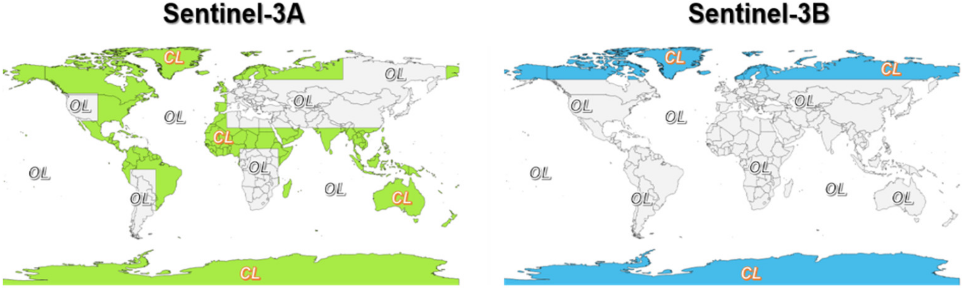
2.1. The S3 Satellites

Sentinel-3A was launched on 16 February 2016 and Sentinel-3B on 25 April 2018. The expected lifetime of each mission is 7.5 years and they are expected to be pursued by the Sentinel-3C and Sentinel-3D missions. Both S3A and S3B have sun-synchronous almost circular orbits with a 98.65° inclination, and therefore, allowing nadir observations up to 81.35° of latitude. This corresponds to a mean altitude of about 815 km above Earth. Such orbits have a 101 min period and are designed so that the satellite ground track repeats over a 27-day cycle. Station keeping maneuvers ensures that the across-track drift with respect to the nominal ground track remains smaller than 1 km [23]. After its commissioning phase, S3B was positioned into a tandem orbit with S3A: it had the same ground track as S3A and overflew it 30 s before. This phase was of great importance for calibration purposes of all the instruments onboard S3 (SRAL, Microwave Radiometer (MWR), Ocean and Land Color Instrument (OLCI) and Sea and Land Surface Temperature Radiometer (SLSTR)). As for the altimetry mission it can also be exploited to allow comparisons between the acquisition modes (Low-Resolution Mode vs. SAR), as well as tracking modes (CL vs. OL), the subject on which this article focuses on.

2.2. The Altimetry Datasets

The principle of altimetry is to emit radio wave pulses and to record the time between the emission and the reception of the reflected echoes. The measured backscatter energy as a function of time is called the waveform. Its shape depends on the characteristics of the surface the radio wave was reflected on, in particular of the surface rugosity. The analysis of a waveform provides valuable information such as the distance between the satellite and the reflecting surface (hereafter range), the amplitude of the backscattered signal (Sigma0), the significant wave height, etc., [18,24,25].

These physical parameters are deduced from the waveform thanks to so-called “retracking” methods that consist of fitting a physical or an empirical model to the waveform. Because the waveform’s shape strongly depends on the reflecting surface characteristics, different retracking algorithms are used on different surfaces (e.g., ocean retracking algorithm Samosa [26] for oceanic surfaces, Offset Center of Gravity (OCOG) for complex shapes resulting from backscattered signals over small water bodies and land).

For an extensive description of the Sentinel-3 Surface Topography Mission refer to [27].

This study uses the Sentinel-3A and Sentinel-3B Level2 Short-Time Critical (STC) 20 Hz data. These data are available within 2–3 days after acquisition in the form of one file per track (different from NRT that are granules, not necessarily identical from one cycle to another). These STC data are used by several projects providing operational monitoring of the inland water levels (e.g., Copernicus Global Land Service, Copernicus Climate Change Service, THEIA/Hydroweb).

The fields used in the study are the backscatter coefficient Sigma0 derived from the OCOG retracking algorithm, as well as the orbit, range (OCOG retracking algorithm) and geophysical corrections necessary to compute the estimated water surface height. The OCOG retracking algorithm has been considered in this study over the other retracking algorithms available in the Payload Data Ground Segment (PDGS) Land products (such as SAMOSA). This choice has been done assuming that OCOG is empirical and should thus provide range estimations with sufficient precision (with respect to the purpose of this study) for most of the water bodies considered, from small rivers to large lakes. As presented in [27] OCOG would be more robust than the ocean retracking algorithm should the waveforms present several peaks.

The higher the backscatter coefficient, the better the reflectivity of the radar wave. As water body surfaces favor reflectivity, a high Sigma0 value has a strong probability to indicate that the altimeter signal was reflected on some water body. The water surface height (WSH) elevation is computed with the following formula: Equation (1): Water surface height estimate calculation from the L2 data.

WSH = altitude − range (OCOG) − corr − geoid

(1)

where altitude is the distance between the satellite and the reference ellipsoid (WGS84), range (OCOG) is the distance (estimated with the OCOG retracking algorithm) between the satellite and the reflective surface returning the radar signal within the altimeter receiving window (whose width is about 60 m for both Sentinel-3A and Sentinel-3B) and corr represents the geophysical corrections. They are to account for the variation of the velocity of the radar wave due to the atmospheric effects as well as the tides (Equation (2)). Geoid is the distance between the reference ellipsoid and the EGM2008 geoid model, and therefore, the water surface height is referenced relatively to the EGM2008 geoid model. All values are extracted from the L2 land PDGS STC datafiles.

The geophysical corrections are computed with the following equation, in which dry corr stands for dry tropospheric correction (ECMWF Gauss model), wet corr for wet tropospheric correction (ECMWF Gauss model), iono corr for ionospheric correction (GIM model), pole tide is provided in the PDGS product as the Wahr85 model and solid earth tide as the Cartwright71 model. Equation (2): Geophysical corrections applied to the range to account for atmospheric and tide effects.

Corr = dry corr + wet corr + iono corr + pole tide + solid earth tide

(2)

2.3. The Open-Loop Tracking Mode, Open-Loop Tracking Command Principle and its Expansion Process

The Sentinel-3 satellites can be operated either in CL or OL tracking mode in different areas as defined by a tracking mode bit. During the S3A/S3B tandem phase, Sentinel-3B was operated in the OL tracking mode over two cycles in the ±60° latitude band overland and in CL outside as illustrated in Figure 1. It was fully operated in CL during the other cycles of the tandem phase. After reaching its nominal orbit, Sentinel-3B OL patches remained the same (an extension of the OL patches overland beyond 60° is planned in summer 2020) and S3B was operated in the OL tracking mode. Regarding Sentinel-3A, the situation is slightly more complex. Until March 2019, S3A was operated in the OL tracking mode overland in the patches presented in Figure 1 and in CL outside. After March 2019, the OL patches were extended to the full ±60° latitude band overland (similarly to S3B).

In OL tracking mode, the altimeter uses an elevation prior uploaded onboard the altimeter to position its receiving window. This information is provided by the OLTC. The first OLTC (called Diode/DEM tracking mode) was implemented in the POSEIDON-3 altimeter on Jason-2 as an experimental mode. The generation process and first inflight validation were described in [28]. The quality and the consistency of the water masks and DEM used for the generation of the targets (altitude and position) were recognized at that time as fundamental for the successful acquisition of data over inland waters.

Collecting such data was also recognized as a difficult task as the target altitudes must be known with an accuracy of around 10 m. Therefore, the first data used (from Generic Mapping Tool (GMT) [29]) were soon replaced by a water mask derived from GlobCover [30] and the ACE2 DEM [31] complemented with targets coming from the THEIA/HydroWeb database [1,6] for the generation of the OLTC that was used during the commissioning of Sentinel-3A in 2016. In addition, around 500 targets were defined over Europe for Sentinel-3A using alternative data and methods [17]. This led to the Sentinel-3A OLTC version 4.2 (v. 4.2) which has been in use until 9 March 2019.

After the validation of the new generation process [17], it was implemented at a larger scale (globally) for hydrology targets only in order to define the version 5.0 (v. 5.0) of the Sentinel-3A OLTC (activated on 9 March 2019) and the version 2.0 (v. 2.0) of the Sentinel-3B OLTC (activated on 27 November 2018). The main differences with respect to the previous process are that separate processing for river targets and lake/reservoir targets and the input data are used. For lakes, we used data from the Global Lake and Wetland Database (GLWD) [32] which provides polygons and reference heights. We also used SRTM Water Body Database (SWBD) [33] and the newly published Global Surface Water Explorer (GSWE) [34] masks for localization of the water bodies and a filtered version of SRTM for reference height. For rivers, the first step is the generation of a network with centerlines of the rivers complemented with their altitude profile. This allowed removing some errors present in the input DEM by taking into account the fact that the river altitude decreases in the downstream direction. A further step is to compute the intersection between the water bodies and the satellite nominal ground tracks. A last but important step is to verify that the generated altitudes are consistent with the altitudes found in major databases of Virtual Stations (VS), defined as the intersection between the satellite ground track and the water bodies from THEIA/HydroWeb [6], G-REALM [7], DAHITI [8], etc. If not, we retain the altitude found in the VS database. Indeed, when working at the global scale with automatic methods, it is not possible to avoid a small fraction of errors (e.g., some reservoirs built after 2000 may not be present in the DEM data nor in the input database of reservoirs and the existing DEM are known to have many sources of errors).

The OLTC thus contains elevation prior specified over the water targets for which some elevation information was available in at least one of the databases presented before. It also contains elevation prior “interpolated” between those targets. In this article, we call “targets for which the OLTC has fine-tuned” the water targets at which the associated OLTC was precisely defined using external databases. Other water targets that are not present in any hydrological database are associated with an elevation prior in the OLTC that comes from the previous closest target, we called them water bodies for which the OLTC is not fine-tuned.

2.4. Further Improvements of the OLTC

In 2020, new OLTC data were generated for Sentinel-3A (OLTCv6.0) and Sentinel-3B (OLTCv3.0). The new Sentinel-3B OLTC was activated on 18 June 2020. After careful examination of the quality of three published databases, it was decided to use the Global Reservoir and Dam Database v. 1.3 (GRaND) [35] and HydroLakes [36] databases that contain more than 10 million lakes instead of GLWD for the generation of the lakes/reservoirs targets. The river network has also been expanded in order to observe smaller rivers (currently larger than 30 m). In addition, the covered zone is extended beyond a latitude of 60°N in order to cover the arctic regions whose observation is considered very important in the climate change context. As the upload of Sentinel-3B OLTCv3.0 is very recent (18 June 2020, OLTC versions and their respective use dates onboard the Sentinel-3 altimeters are detailed on https://www.altimetry-hydro.eu/) at the time of writing and Sentinel-3A OLTCv6.0 is not yet uploaded (

Table 1. Description of successive Open-Loop Tracking Command (OLTC) versions on Sentinel-3A and Sentinel-3B. The versions used in the analysis presented in this article are in bold.

Mission	OLTC Version	Date of Activation	Number of Hydro Targets (Total)	Number of Hydro Targets by Type: Rivers/Lakes/Reservoirs/Glaciers, Identified for OLTC Definition	Geographical Area Covered in Open-Loop Mode Over Land
Sentinel-3A	V4.1	18 April 2016	2253	2007/246/-/-	4 areas of interest
Sentinel-3A	V4.2	24 May 2016	2253	2007/246/-/-	4 areas of interest
Sentinel-3B	V1.0 (tandem)	6 June 2018	2253	2007/246/-/-	Global
Sentinel-3B	V2.0	27 November 2018	32,515	17,016/14,245/1231/23	Latitudes inside ± 60°
Sentinel-3A	V5.0	9 March 2019	33,261	17,409/14,427/1386/39	Latitudes inside ±60°
Sentinel-3B	V3.0	18 June 2020	73,629	21,719/47,738/4149/23	Global
Sentinel-3A	V6.0	September 2020 (TBC)	74,050	20,100/47,637/4262/51	Global

), the discussion on the benefits of these last versions is left for a future publication.

An important modification in these new OLTC tables is that a target altitude is explicitly defined for every point overland. This was not the case in previous OLTC. If no hydrology target was identified, the position of the altimeter tracking window was imposed by the previous target. This behavior explains why a waterbody that was not defined in the OLTC could only be observed by chance. In the 2020 OLTC, when there is no hydrology target identified in the vicinity of a point, an altitude is defined using the DEM altitude. The choice of the altitude maximizes the chance to observe a waterbody (choice of the altitude at the bottom of the valleys), provided the DEM is correct. The target altitude is kept constant over around 20 km in order to respect altimeter memory constraints onboard Sentinel-3A and Sentinel-3B. These constraints will not be present for Sentinel-3C and Sentinel-3D thanks to a larger onboard memory. It must be noted that the prior altitude is also kept constant around fine-tuned targets. If two fine-tuned targets are closer than 6 km for rivers and the prior altitude difference between the two targets is higher than 5 m, the prior altitude is changed at the middle point. This method allows the observation of close targets with high altitude differences while keeping enough data points around each target for the retracker processing.

3. Methods

In order to compare the performances of the tracking modes, this paper makes use of the data acquired during the tandem phase during which S3B was circulated between various configurations while S3A remained as the reference as presented in Figure 2. The performance improvements brought by the OLTC updates are evaluated on another period, longer than the tandem phase, by comparing one year of data acquired by S3A in CL or in OL with the OLTCv4.2 with one year of data acquired with OLTCv5.0 in OL.

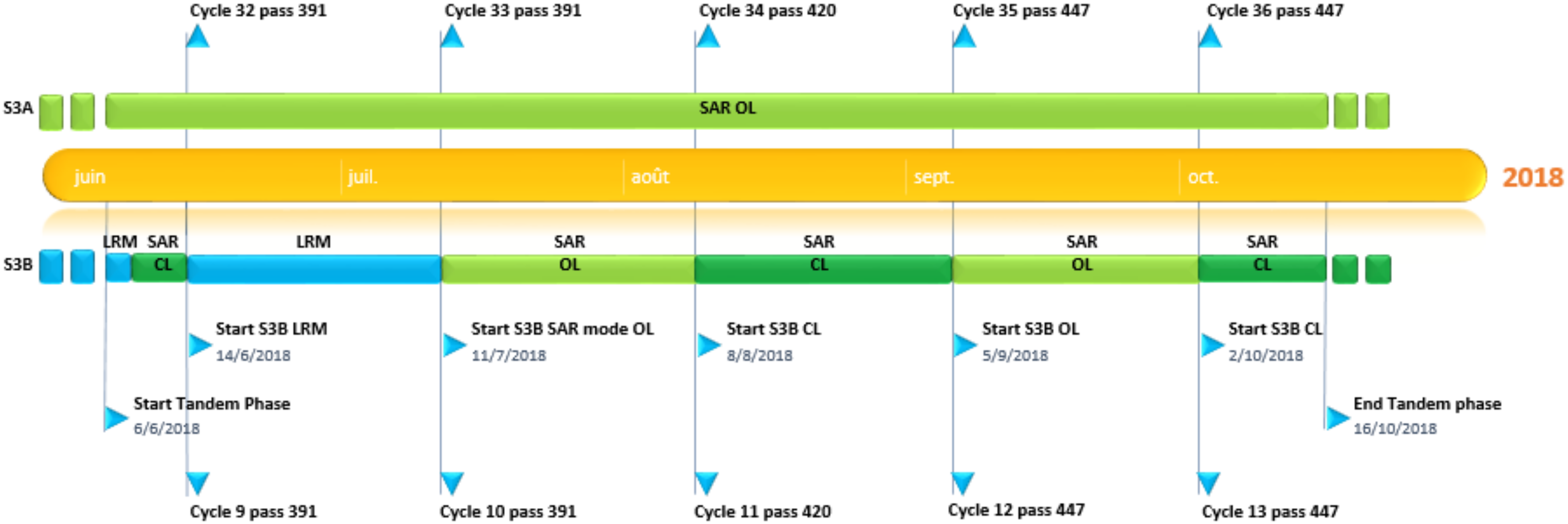
3.1. Timeline and Use of the Tandem Phase Data for the Different Purposes

Regarding the comparison of the OL and CL tracking modes, the period covering S3B Cycle 11 Pass 420 to Cycle 12 Pass 446 is of interest. Indeed, S3B was in the CL tracking mode, while over the same period S3A, over some regions, was in the OL tracking mode. This corresponds to S3A to Cycle 34 Pass 420 to Cycle 35 Pass 446.

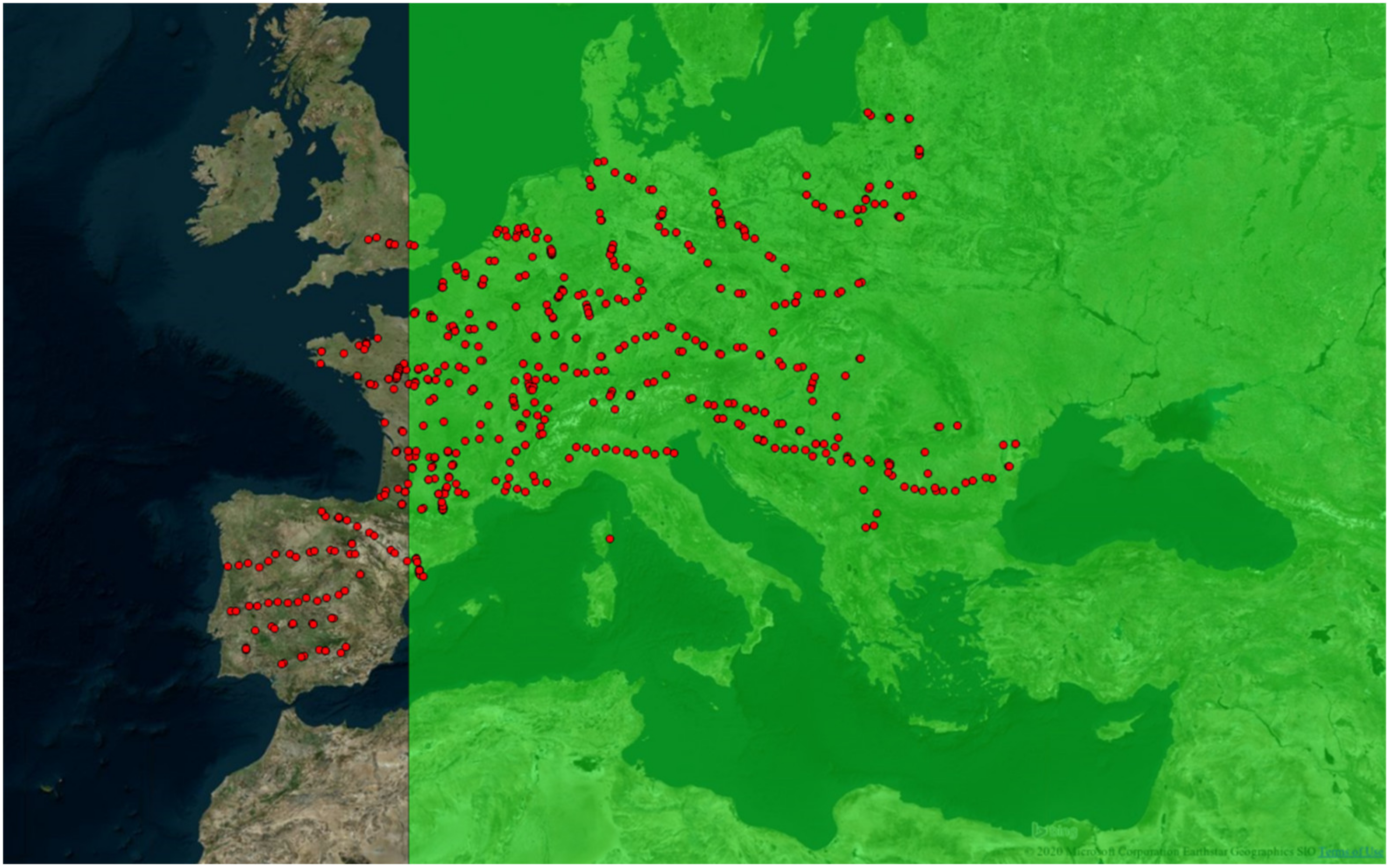
3.2. Target Selection

To ensure the comparison of the acquisition and tracking modes in terms of their capabilities over water surfaces, the altimetric along-track data were extracted in polygons centered around hydrological targets. To assess the performances of the OL tracking mode we considered those targets for which a specifically tuned elevation prior in the OLTCv5.0 was provided.

The database of the centers of the hydrological targets used as references for the OLTC is accessible on https://www.altimetry-hydro.eu/ and is regularly updated based on hydrologists’ feedback and their compilation by CNES. Polygons were defined around these targets as a 3 × 3 km square on rivers, along-track-oriented, and along all the water transects (intersection of theoretical ground track and water body extension), also with a 3 km buffer in the across-track direction, for the lakes. The extraction within the OLTC polygons is interesting as these polygons are not restricted to the extent of the water bodies for the smallest ones but rather to a 3 km long box along the satellite track, centered on the water target. This is of particular interest to consider such extended polygons especially around small lakes or rivers for which the transects are shorter than 300 m, since for such targets, no 20 Hz data might have its associated nadir point positioned within the water body although the instrument footprint embraces it. Off-nadir measurements are, therefore, of great interest to tackle the smallest water bodies.

3.3. Editing Performed on the 20 Hz Data

In the perspective of the use of the Level-2 PDGS land products in the Level-3 services, it is also relevant to assess the impact of the OL and CL tracking modes on the estimation of the water level over the transects (defined as the crossing of one ground track with a water body). To that respect, the following editing algorithm is used to select the 20 Hz data and compute the Level-3-like water level estimate over one transect and their associated uncertainty. This algorithm is the one used in the Copernicus Global Land Water Level Service (described in this Level-3 product Algorithm Theoretical Basis Document (ATBD) [37]), with a few minor simplifications. It is described below:

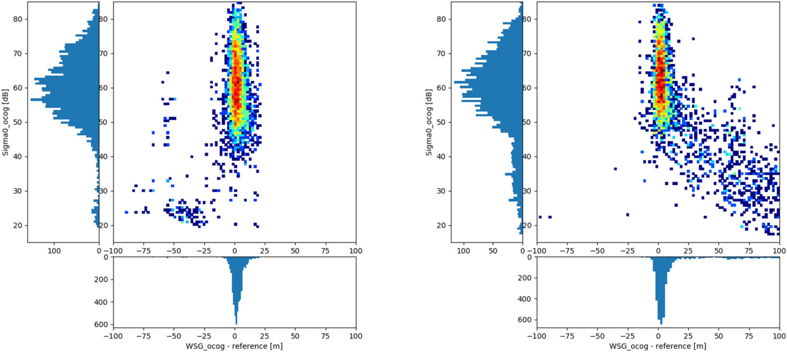
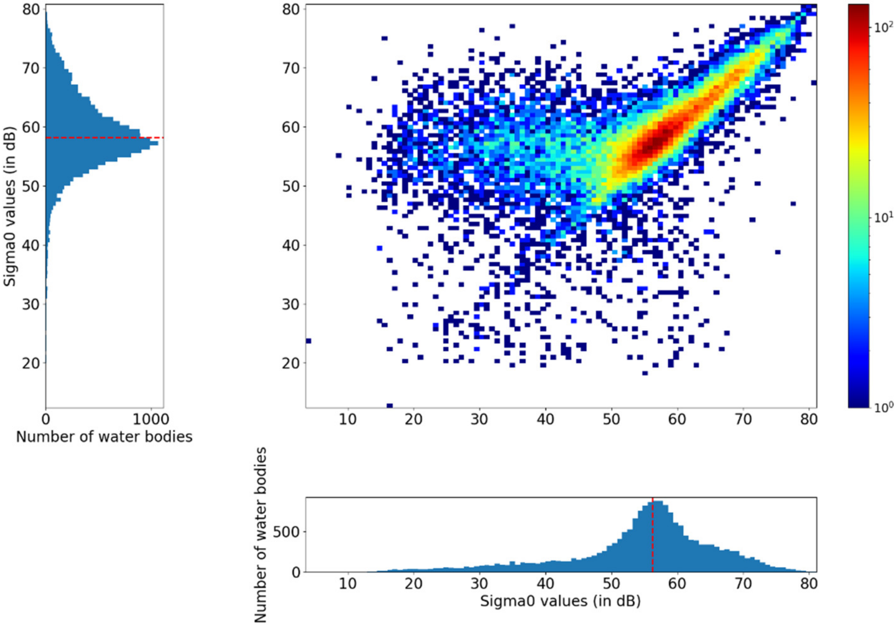
• Sigma0 OCOG thresholding:

  ○

  Only 20 Hz points with a Sigma0 OCOG value higher than 55 dB over rivers and 45 dB over lakes are selected. The thresholds were empirically estimated based on the Sigma0 OCOG distributions over these two types of targets. We point out that these thresholds correspond to the Sigma0 OCOG values of the L2 S3 PDGS Land products prior to the L2 processing baseline IPF-SM-2 v. 6.18 that was installed in January 2020. This processing baseline introduced a −18 dB (−10 log(64) [38]) correction on all Sigma0 OCOG values (switch on Cycle 53 Pass 116 for S3A and Cycle 34 Pass 598 for S3B of the STC products). This editing can be applied for more recent data by shifting the Sigma0 OCOG thresholds by about −18 dB.

  ○

  Among the points selected in the previous step, the 50% percentile of the points presenting the highest Sigma0 OCOG values is then selected.

• Criteria on WSH standard dispersion:

  ○

  The median value of the selected 20 Hz points over the same transect is computed.

  ○

  Only 20 Hz points within 10 m of the median value are selected.

  ○

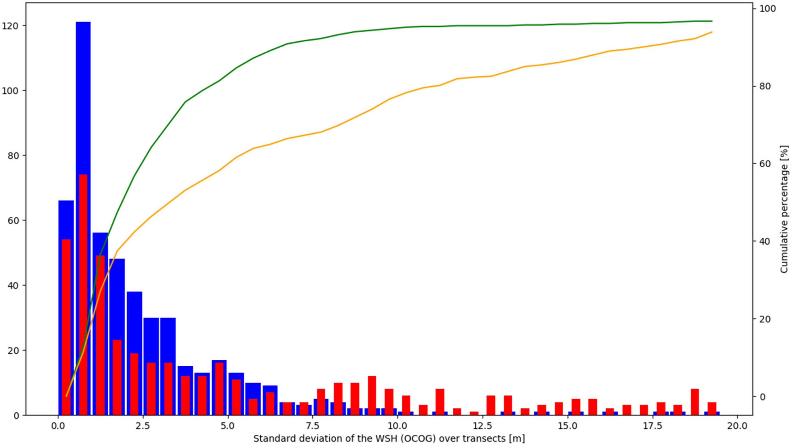
  The standard deviation ($\sigma =\frac{1}{n}{{\displaystyle \sum }}_{i=1}^n\sqrt{{\left(x_i-\overline{x}\right)}^2}$) of the selected 20 Hz points over a similar transect are computed.

  ○

  Only 20 Hz points within three times the standard deviation around the median value are selected.

  ○

  The final “compressed” value of the WSH estimate of the transect is computed as the median of the selected 20 Hz points. The standard deviation of the valid points is also computed (denoted as ${\sigma }_v$).

4. Results

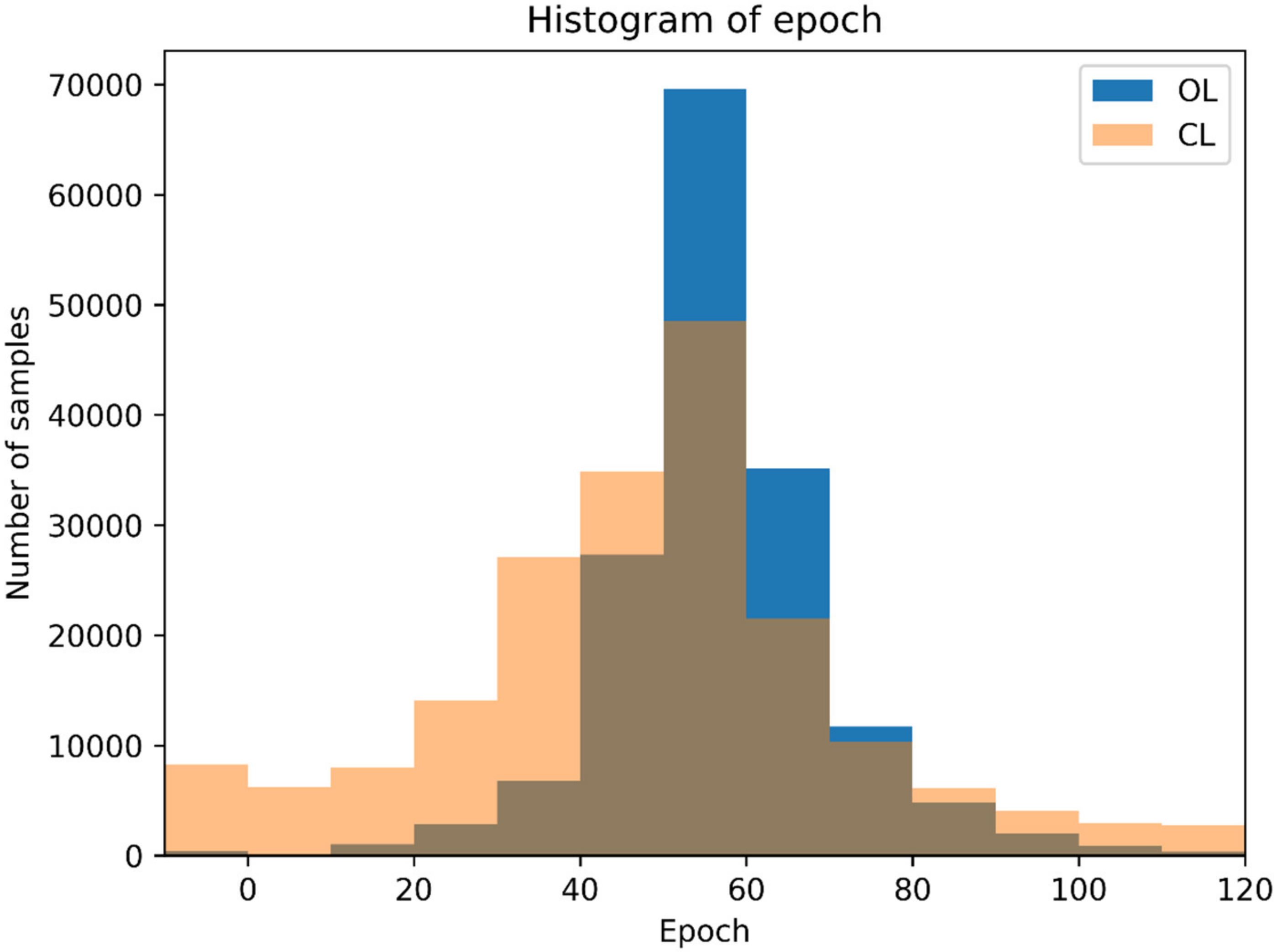
4.1. Improvements of the Retrievals in OL Compared to the CL Tracking Mode

4.1.1. Exploiting the Tandem Phase to Compare Similar Scenes in CL and OL

During the S3A/S3B tandem phase, a period of one cycle was covered by S3A in the OL tracking mode and S3B in the CL tracking mode. This provides a unique opportunity to assess the performances of each of these two modes. In the OL mode, the altimeter uses an a priori elevation, provided by the OLTC, to set up its acquisition window, contrary to the CL mode where it adapts the window positioning to track the maximum backscattered energy based on the previous acquisitions. The OL/CL comparisons in this section are only performed over the OLTCv4.2 river targets over Europe. It is indeed not relevant to assess the quality of the OLTC to focus on water targets for which it was not precisely set. Data are only extracted within the 3 × 3 km polygons (hereafter OLTCv4.2 polygons) defined around the Virtual Stations (intersection between S3A ground tracks and rivers) for which the OLTC prior was fine-tuned (as described in Section 2.3; Figure 3). In this section, the analysis is only performed over rivers so that the discussion on the 20 Hz points is not dominated by the large number of points over the largest lakes. There are 515 such OLTCv4.2 Virtual Stations. An example of such an extraction is presented in Figure 4, which shows the S3A and S3B 20 Hz points extracted within a Virtual Station polygon. The S3A data (western track) are observed in the OL mode and present much higher Sigma0 OCOG values than the S3B data (eastern track) observed in the CL mode.

The backscatter coefficient is an indicator of the reflectivity of the reflecting surfaces, and therefore, an indicator of the water tracking and the water surface height estimates are compared between S3A and S3B over the OLTCv4.2 polygons.

First, data availability is compared between the two OL and CL tracking modes. The percentages of acquired data (not necessarily valid) are larger in OL. Indeed, there is no missing 20 Hz data over 513 out of the 515 OLTCv4.2 stations with S3A (the two remaining stations being on a track for which no observations were recorded). These 20 Hz data consist of 4666 points for S3A while it drops to 4232 for S3B: in the CL mode, there is about 9.3% missing data. Thanks to the use of a prior elevation in the OL tracking mode, the tracking window is instantaneously adapted, in the CL tracking mode, however, some adaptation time is needed when the backscattered signal is lost. The percentage of invalid data (missing in the L2 products as well as data points for which the range in the L2 products is set to the default value, i.e., NaN) in OL is 1.1% while it reaches 12% in CL). As shown in [15], in Figure 5, when S3A and S3B both were operated in the OL tracking mode during the tandem phase, the waveforms obtained by both instruments were very similar showing the consistency between the two altimeters. The significant difference in terms of data availability we point out between S3A and S3B during the tandem phase when they operated in different tracking modes can, therefore, be attributed to the CL tracking mode.

The validity of the available data is then assessed. The fact that these values correspond to tracked water targets is now discussed. As presented in Figure 5, in the CL tracking mode, the Sigma0 OCOG distribution presents a tail at low (<45 dB) values. In OL, the distribution is much better centered around high values. This means that the CL was hooked on low reflectivity targets, more likely not to be water, when the OL was tracking higher reflectivity surfaces, more likely to be water. The density plot in Figure 5 represents the density of 20 Hz points as a function of the backscattered energy and as a function of the difference between the WSH estimate and the WSH reference elevation. Reference elevation is taken as the tracking command that was set in the OLTCv4.2 (from hydrological priors). The “WSH—reference elevation” value, therefore, indicates whether the altimeter was tracking the desired waterbody or not. We point out that rivers exhibit low and high regimes throughout a year, and therefore, a correct measurement can deviate from the reference value but this difference remains smaller than 10 m. Low differences (<10 m) are associated with high Sigma0 values as expected. This diagnosis enables checking whether ranges associated with high Sigma0 values are indeed associated with water bodies.

As seen in the density plot (Figure 5, left), in the OL tracking mode, the vast majority of 20 Hz points present an absolute difference between the estimated WSH and the reference elevation (|WSH-reference elevation| values) lower than 10 m associated with Sigma0 values > 45 dB. These high sigma0 values show that the retracked range is indeed associated with a highly reflective target corresponding to the water surface. It proves that the S3A onboard OLTC was properly set up to track the water free surface. Few points (2.6%) present low (<45 dB) Sigma0 and |WSH-reference elevation| values larger than 20m indicating that the OLTC was not suited to track the water body. Some points present Sigma0 values higher than 45 dB and |WSH-reference| values around 60 m possibly indicating that either the OLTC was not well adapted or the range to another water body within the altimeter footprint has been retracked.

Figure 5 (right) shows that CL properly tracks a large fraction of the water bodies considered in this study (Sigma0 > 45 dB and |WSH-reference elevation| value < 20 m) but also hooks on much more other reflecting targets (|WSH-reference elevation| > 20 m) either not at the altimeter nadir or with low reflectivity (Sigma0 < 45 dB). Of the points, 12.6% present a low (<45 dB) Sigma0 and |WSH-reference elevation| values larger than 20 m. It is worth pointing out that almost all of these “outlier” measurements are associated with targets with a higher elevation than the studied water body (positive WSH-reference value), meaning that the CL is tracking the hills rather than the rivers or reservoirs lying on the bottom of the valleys, which would be more useful.

Figure 6 presents the inverse cumulative distribution function of |WSH-reference elevation| (|…| are used to refer to the absolute value). It, therefore, represents the percentage of points for which the |WSH-reference elevation| difference is larger than the values in the X-axis. This percentage decreases much faster in OL than in CL which is consistent with the results shown in the WSH-reference histograms in Figure 5. Half the points have a |WSH-reference elevation| value lower than 2.8 m in OL and 4.2 m in CL. The percentages of points for which |WSH-reference elevation| > 60 m is 0.4% in OL and 16.2% in CL. The remaining 0.4% in OL is associated with extraction areas over polygons where the OLTCv4.2 was not properly set up or where water was missing. The 16.2% points in CL give an order of magnitude of the number of cases where the altimeter hooked on another reflective surface rather than on the water body present at nadir.

When considering individual 20 Hz points the benefits of the OL tracking mode with a well-set OLTC clearly are shown with respect to the CL tracking mode. Level-3 water level satellite products use these 20 Hz points and perform different editing to select the best-suited high-frequency points to compute one value of water level estimate (and associated uncertainty for some products) over one transect (=water body crossing). This means that one single water level estimate is computed from the S3A 20 Hz points in Figure 4 (and similarly for S3B). From the perspective of the use of the Level-2 PDGS land products in these Level-3 services, it is also relevant to assess the impact of the OL/CL tracking modes on the estimation of the water level over the transects. The algorithm described in Section 3.3 is used to perform the editing on 20 Hz data and compute the WSH estimate from the valid (nonedited) 20 Hz points across the transects and the associated dispersion of these selected valid 20 Hz points.

The standard deviation of the WSH estimates computed from all the 20 Hz points of each transect (Figure 7) is compared between the OL and CL tracking modes. This allows comparing the precision of the WSH median estimate per transect. First, without editing, the median over all transects of the standard deviation per transect is of the order of 1.7 m in OL and 3.1 m in CL. This shows WSH transect dispersion is smaller in OL than in CL, and also points out the need for dedicated editing on the 20 Hz points before using them.

With the Level-3-like editing (Section 3.3), only 371 stations present at least two valid 20 Hz points in CL which is 25% smaller than the 494 stations presenting at least two valid 20 Hz points in OL. After editing, the median standard deviation per transect is of the order of 42.8 cm in OL and 37.8 cm in CL. The slightly smaller value after editing in CL is explained by the fact that CL presents less valid (with respect to the editing presented in Section 3.3) 20 Hz points and moreover only hooks on targets presenting low surrounding terrain elevation gradients as presented in Figure 8 while in OL more water targets are observed in those complex terrain situations. Figure 8 shows that the water targets over which no valid data was found in CL are mainly situated in mountainous or hilly areas where the tracker does not have sufficient time to adapt to the terrain elevation changes and to position the receiving window to track the backscattered radar signal.

Therefore, from a Level-3 water level product perspective, the OL tracking mode allows considering more targets (25% in this study case) than would have been with the CL tracking mode, without compromising the precision of the water level estimates.

4.1.2. Sentinel-3A Switch from CL to OL Tracking Modes

The previous section emphasized the potential of the OL tracking mode with respect to the CL tracking mode to detect water and monitor water surface heights. This section presents the benefits of extending the OL tracking mode area in S3A from the continental patches (Figure 1, left) to a full ±60° latitude band (similar to the one used by S3B during the OL cycle of the tandem phase as illustrated in Figure 1, right). Over this area switched from CL to OL in March 2019, the OLTC was fine-tuned for 18,724 targets. Those targets were observed in CL before Cycle 43.

Sentinel-3A L2 data were extracted over these 18,724 OLTCv5.0 polygons, over 13 cycles covered in CL (Cycles 29 to 41) and 13 cycles covered in OL (Cycles 43 to 55). The distribution of the median over each period of the Sigma0 OCOG values per water body is presented in Figure 9. In CL tracking mode, the median per target of Sigma0 OCOG presents a tail at low values, about 15% of the targets present a median value lower than 45 dB was defined as the threshold for water surface detection cut off. This means that no water is detected on these targets. On the other hand, in the OL tracking mode, only 5% of the targets present a median value lower than 45 dB. They are either large lakes for which waves play a significant role in reducing the backscattered energy or targets for which the OLTC is not yet well suited for the receiving window to be correctly positioned to track the backscattered radar signal. Over 10% of the 18,724 targets considered, switching to CL the tracking mode allowed increasing the median values of Sigma0, confirming the altimeter now better tracks these water targets. The scatter plot in Figure 9 represents the density of water bodies as a function of the median Sigma0 OCOG per water body before March 2019 (CL in the horizontal axis) and after (OL in the vertical axis). It shows that after switching to the OL tracking mode, the 10% gain in the number of water bodies for which water is now tracked comes at the cost of a small number of degradations in water detection.

The same editing as presented in Section 3.3 is then applied on the L2 20 Hz data and the median and standard deviation of the WSH per transect are computed. The median of the WSH standard deviation is then calculated for each target, over the CL and OL tracking mode periods. The distributions for both periods are represented in Figure 10. The distributions are very similar as shown by the cumulative distribution functions. This means that once water is tracked by the altimeter, OL does not significantly improve the WSH estimate precision over CL tracking mode. Nevertheless, in the CL mode 2.1% more targets (16,656 versus 16,314) are tracked at least over 1 cycle (for the computation of the median per target of the SWH standard deviation). This result appears different from the 25% more transects obtained in OL during the tandem phase (Section 4.1.1). The areas covered in CL by S3A before March 2019 were mainly areas with weak elevation gradient (S3A OL patches positions before March 2019 in Figure 1, left). The tracker did not need as many significant elevation changes in the positioning of the tracking window as in mountainous areas already covered in OL before March 2019. The lower elevation gradients in the areas where S3A was operated in CL before March 2019 explains why the CL mode tracks, at least over one cycle, as many targets as the OL mode.

The raw number of targets for which WSH is estimated at least once after editing should be considered carefully. Figure 11 presents the distribution of the number of cycles per target used for the calculation of the medians displayed in the histograms of Figure 10. It appears, as shown by the cumulative distribution function, that the targets, observed in OL, present one more valid cycle (i.e., a cycle for which there are at least two valid 20 Hz points over a transect after applying the editing algorithm) on which to estimate WSH than with the CL tracking mode.

The larger number of cycles in OL for which S3A provided a valid WSH estimate compared to CL confirms the results obtained by comparing OL and CL tracking modes during the tandem phase (Section 4.1.1). The benefits from the OL tracking mode appear worldwide but are more significant over areas with significant elevation gradients.

4.2. Benefits of the Improvements of the Open-Loop Tracking Command

This section focuses on showing the improvements brought by the OLTC updates onboard S3A and S3B as described in Section 2.3. As the OLTCv6.0, for S3A, and OLTCv3.0, for S3B, were recently updated at the time of writing, in this article, we focus on the benefits of version 5.0 compared to version 4.2 of the S3A OLTC. The upload of the OLTCv5.0 took place between 1 March 2019 and 9 March 2019 (Cycle 42 Pass 100 to Cycle 42 Pass 317 of S3A, during this period S3A tracking mode was switched to CL). In order to avoid this CL period that occurred during the OLTC update, the comparison between the S3A OLTC versions are, therefore, performed on the 13 cycles 29 to 41 using OLTCv4.2 and on the 13 cycles 43 to 55 using OLTCv5.0.

The comparisons between the OLTC versions are only performed over the areas for which OLTCv5.0 was fine-tuned, since the OLTC was not precisely set (it was interpolated) outside of these polygons neither in OLTCv4.2 nor in OLTCv5.0. Only the OLTCv5.0 targets situated in the areas where S3A was in OL during the use of OLTCv4.2 (white areas in Figure 1) are considered in order to compare the effect of updating the OLTC version and not having CL vs. OL effects (already detailed in Section 4.1) to account for.

Two study cases are presented:

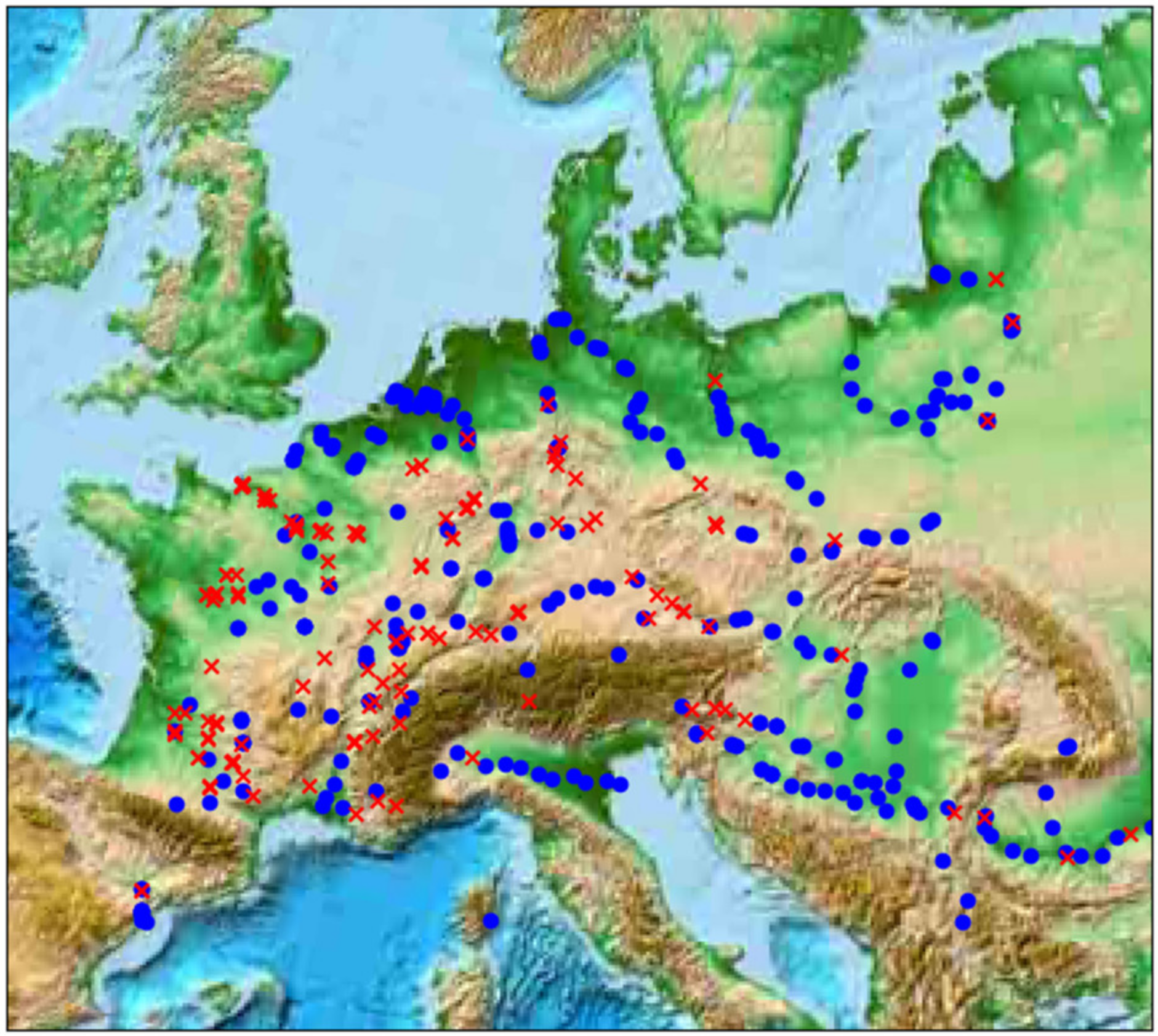
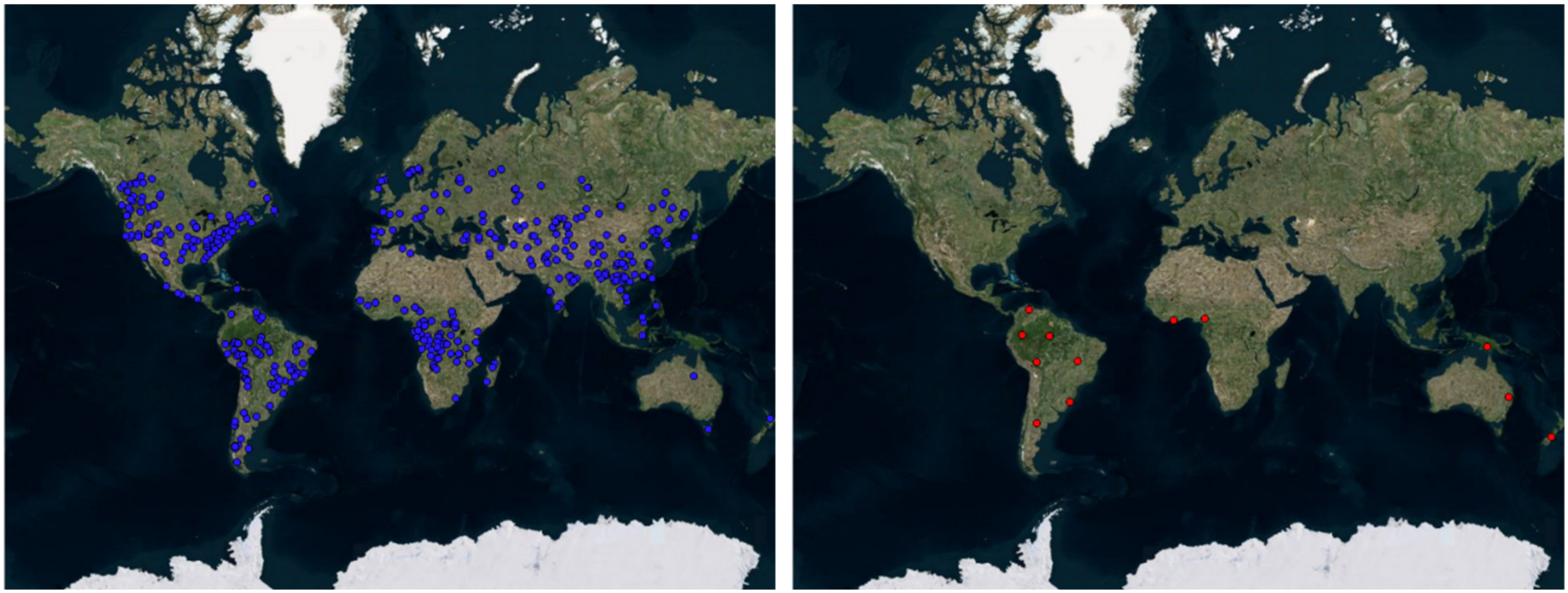
• Comparison of the S3A performances in OL over targets over which the OLTC was fine-tuned already in OLTCv4.2. This is mainly a sanity check diagnosis; no particular difference is expected (unless the OLTC is erroneous in one OLTC version).
• Comparison of the S3A performances in OL over targets over which no fine-tuned OLTC value (therefore the OLTC for these targets consisted of an interpolation) was defined in OLTCv4.2. This study case is expected to emphasize the improvements, in terms of water tracking and water level estimations, by switching from an “interpolated” OLTC to a tuned one.

4.2.1. Over Targets Already Having a Fine-Tuned Elevation Prior in OLTCv4.2

Among the 33,261 OLTCv5.0 targets over which the OLTC was fine-tuned (over some water bodies from external databases as detailed in Section 2.3), 14,537 are in the continental patches over which S3A was already operated in OL before March 2019 (Figure 1, left). In total, 1299 of these 14,537 targets were already having fine-tuned elevation in OLTCv4.2. The current section, therefore, focuses on those 1299 targets (rivers and lakes).

The 20 Hz Sigma0 OCOG values were extracted over each target, and their median per target was computed over the OLTCv4.2 period as well as over the OLTCv5.0 period. The scatter plot in Figure 12 presents the joint distribution of these Sigma0 OCOG medians over both periods. The histograms on the axis present the distribution with each version of the OLTC. The low Sigma0 OCOG (<45 dB) tail in v. 4.2 shows that the OLTC over some targets was not appropriate to properly track the water, this represented less than 10% of the targets in OLTCv4.2. This has been improved in OLTCv5.0 with less than 3% of targets where the median Sigma0 OCOG is lower than 45 dB.

The standard deviation of the WSH estimates computed from all the 20 Hz points of each transect is computed for each cycle, and then, its median is computed over both the OLTCv4.2 period and the OLTCv5.0 period for each transect. Figure 13 presents the distribution of both these medians. The distributions are very similar (50% percentile = 17 cm and 17 cm, meaning that for half of the targets the valid 20 Hz data present a 17 cm dispersion across the water bodies, 95% percentile = 85 cm and 86 cm over, respectively, the OLTC v. 4.2 and v. 5.0 periods which shows that the dispersion is also the same over the 5% of the targets presenting the largest dispersion) meaning the precision of the WSH estimates is similar for the targets tracked with a fine-tuned OLTC in both v. 4.2 and v. 5.0. In total, 1200 transects were tracked in v. 4.2 and 1235 in v. 5.0; this 2.9% increase in the number of tracked targets is due to the improvement in the OLTC between the two versions.

As expected, the OLTCv4.2 to v. 5.0 did not have a major impact on the targets for which a fine-tuned OLTC was already present in v. 4.2. The improvement mainly concerned targets for which the OLTC was not adapted.

4.2.2. Over Targets Without a Fine-Tuned Elevation Prior in OLTCv4.2 (but Nevertheless Observed with the OL Tracking Mode)

Among the 33,261 OLTCv5.0 targets over which the OLTC was fine-tuned, 14,537 are in the continental patches over which S3A was already operated in OL before March 2019. In total, 13,238 of these 14,537 targets did not already have a fine-tuned elevation prior in OLTCv4.2. The current section focuses on those 13,238 targets (rivers and lakes).

The 20 Hz Sigma0 OCOG values were extracted over each target, and their median per target was computed over the OLTCv4.2 period as well as over the OLTCv5.0 period. Figure 14 presents the joint distribution of these Sigma0 OCOG medians in both OLTCv4.2 and OLTCv5.0. The two distributions are very different, the one from the OLTCv4.2 points exhibits an important tail for values lower than 45 dB which represents about 22% of the transects while this number drops to about 7% in OLTCv5.0. As shown by the density plot, the vast majority of the targets for which the Sigma0 0C0G value was lower than 45 dB in OLTCv4.2 present values higher than 45 dB in OLTCv5.0. This comes at the cost of minor degradations (points below the first bisector). As the OLTC was not specifically tuned in v. 4.2 for all the considered targets it is not surprising to have such a percentage of low Sigma0 transects. It is, nevertheless, worth pointing out that more than 75% of the transects for which the OLTC was not tuned in v. 4.2 present a high Sigma0 distribution similar to v. 5.0. This means that the OLTC does not have to be specified for all water bodies but rather when there are elevation changes larger than the tracking window size (about 60 m).

Ref. [17] have used Jason-3 data and “Banque Hydro” in situ measurements to show that a significant Sigma0 increase was linked with differences between the altimetric WSH and the OLTC elevations (that were validated on “Banque Hydro” in situ data) smaller than 10 m. This supports the use of high sigma0 values as a prior for ensuring that the altimeter tracks the right water target defined in the OLTC.

The impact in terms of WSH estimate precision is also assessed by comparing the distribution of the median per water body of the SWH standard deviation along the transects after editing on the 20 Hz points (Figure 15), considering only rivers to assess the impact on the smallest targets. Improvements in the OLTC resulted in an increase in the number of river targets over which water level is estimated after the editing: from 5788 in OLTCv4.2 to 7553 in OLTCv5.0, a 30.5% increase. The cumulative distribution functions are different, in particular, the value of the median per water body of the WSH standard deviation at which 90% of the population is reached in v. 4.2 is 77 cm while it is 96 cm in v. 5.0. To understand this difference, the distributions were then plotted considering only the rivers having valid points over both the v. 4.2 and v. 5.0 periods (Figure 16). This shows that when considering exactly the same water bodies, both cumulative distribution functions are similar. Therefore, as long as water is tracked, the precision in the water level estimate is not determined by the OLTC precision. It is expected that Virtual Stations which are tracked in the OLTCv5.0 and not in the OLTVv4.2 are in regions which are more difficult to retrack.

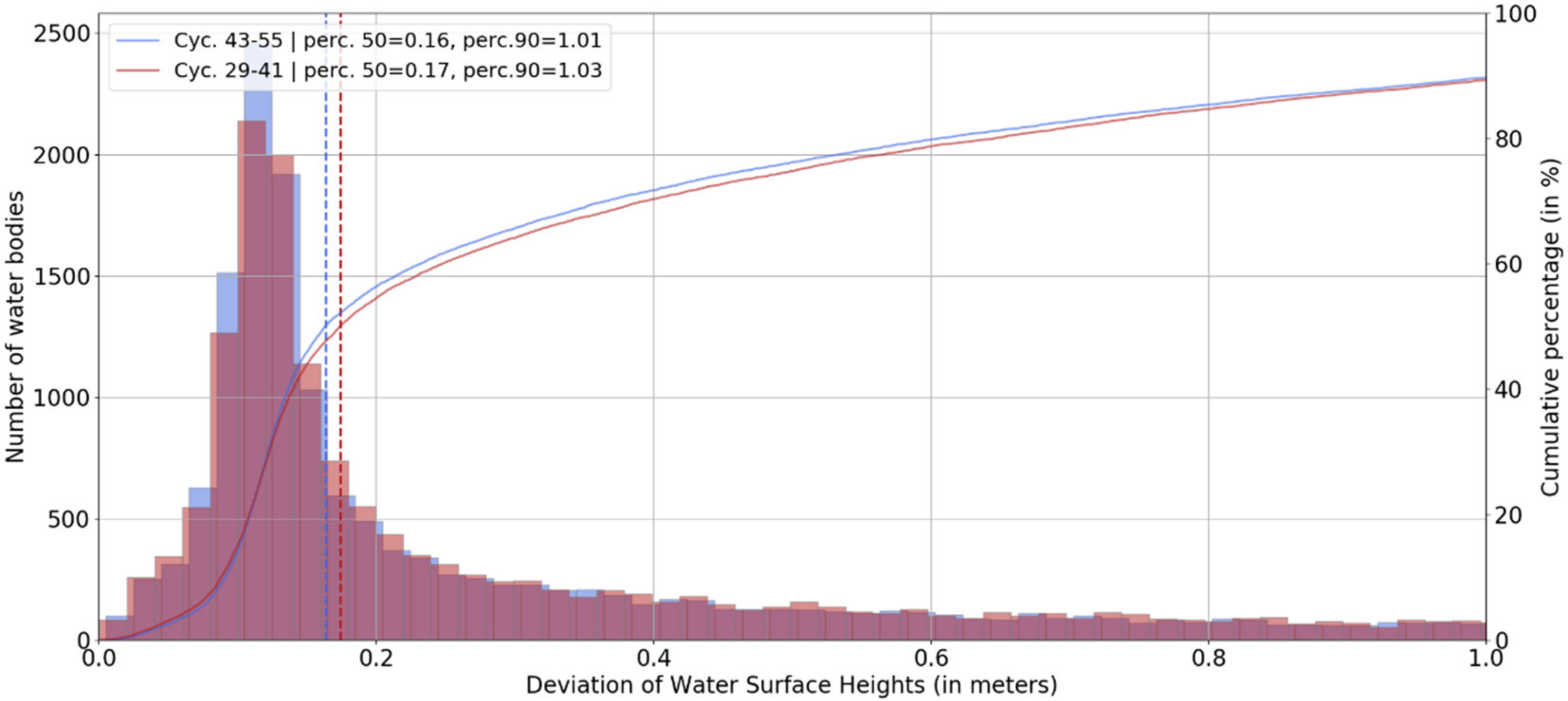
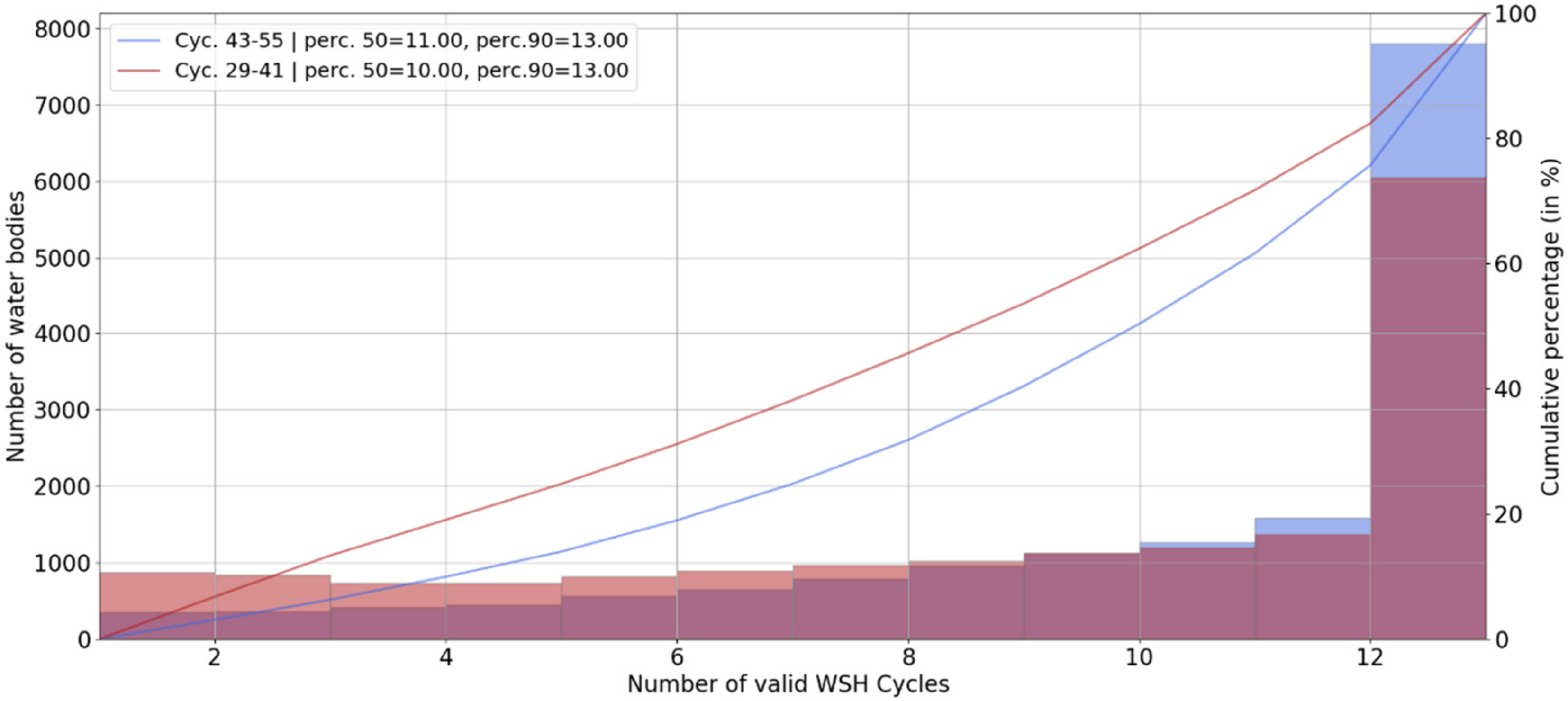
4.2.3. Global v. 4.2 to v. 5.0 Improvements

To determine the water targets where the OLTC significantly affects water detection, the median and per water body of the Sigma0 OCOG values have been compared between over the OLTCv4.2 and OLTCv5.0 periods. Those periods consist of Cycles 29 to 41 for OLTCv4.2 and 43 to 55 for OLTCv5.0. The water bodies used consist of all the targets for which OLTCv5.0 is fine-tuned (33,261 polygons).

A significant improvement in terms of water detection is defined for each target as a Sigma0 median value increase by more than 30 dB and a Sigma0 median value over the OLTCv5.0 period higher than 45 dB (Equation (3)). A degradation is defined as a Sigma0 median value decrease by more than 30 dB and a Sigma0 median value over the OLTCv4.2 period higher than 45 dB (Equation (4)). The 45 dB threshold was set based on the sigma0 distribution in OLTCv5.0 -which is used as a reference in the present comparison- (Figure 14) for which there are only 10% of the water targets presenting smaller values than 45 dB. The 30 dB requirement on the Sigma0 OCOG difference is motivated by the length of the tail of the distribution of the Sigma0 OCOG in OLTCv4.2 (Figure 14). Equation (3): Significant improvement criterion for water detection between OLTCv4.2 and OLTCv5.0 based on the Sigma0 values. $\overline{{\sigma }_{0v4}}$ and $\overline{{\sigma }_{0v5}}$ refer to the Sigma0 median values for a specific VS during the OLTC v. 4.2 and v. 5.0, respectively. Such calculation is performed for each Virtual Station (VS) to estimate whether water detection was improved or not. Equation (4): Significant regression criterion for water detection between OLTCv4.2 and OLTCv5.0 based on the Sigma0 values. $\overline{{\sigma }_{0v4}}$ and $\overline{{\sigma }_{0v5}}$ refer to the Sigma0 median values for a specific VS during the OLTC v. 4.2 and v. 5.0, respectively. Such calculation is performed for each VS to estimate whether water detection was improved or not.

$$\overline{{\sigma }_{0v5}}- \overline{{\sigma }_{0v4}}>30\mathrm{dB} \mathrm{and} \overline{{\sigma }_{0v5}}>45\mathrm{dB}$$

(3)

(4)

Figure 17 presents the locations of the significantly improved and degraded targets. The first category with 445 targets is much larger than the second (12 points). It shows a significant improvement at the cost of few regressions. Significant improvements were noted, for example over the San Salvador reservoir (Spain) as a result of the OLTC improvement. The erroneous OLTC value in OLTCv4.2 to track the water was pointed out in [39] and corrected in OLTCv5.0. Other examples of such water detection improvements as well as degradations are presented in Figure 18. Examples of the OLTC elevation prior importance to obtain consistent WSH time-series can be seen. The improved station on the Tocantins river (in Figure 18, left) shows inconsistent WSH value with high standard deviation in OLTCv4.2 and consistent WSH values, making the annual hydrological cycle appear, with a small standard deviation in OLTCv5.0. The use of the Open-Loop tracking mode with a good elevation prior now allows the water detection over this VS. High Sigma0 OCOG values are obtained as well as consistent WSH values, highlighting the Sigma0 relevance as an indicator of water detection and to perform the editing on the 20 Hz data. In the right plot, the Sigma0 OCOG values significantly decreased after OLTCv5.0 upload in March 2019 which is one of the few examples of loss of surface water tracking after an OLTC update.

5. Discussion

In this section, results are discussed, and potential limitations of the study cases are pointed out.

Comparisons over the tandem phase between the CL and OL tracking modes emphasized that about 25% more stations are tracked in OL. To that respect, the OL tracking mode, in combination with successive OLTC updates, allows obtaining data over areas that were inaccessible with the CL tracking mode due to the terrain’s important elevation gradients (e.g., [1]). From a Level-3 water level product point of view, the improvement brought by the OL tracking mode mainly resides in the number of targets tracked and not in the precision of the WSH estimate provided by the 20 Hz valid data. This is an important point as further improvements of the OLTC are possible and, actually, are already planned.

As the waveform shape and maximum power are good indicators of data quality over inland water, as reminded in [19], the correct positioning of the waveforms is investigated. Figure 19 represents the histogram of the position of the waveforms leading edge within the receiving window. It shows that the centering of the waveforms is much better when the altimeter is in the OL mode. The data are extracted from Sentinel-3A datasets over six cycles (29 to 34 in 2018) when the altimeter was operated in the CL mode and five cycles (43 to 47 in 2019) when it was in the OL mode. These datasets cover the end of the spring and summer period.

The much better centering of waveforms in the OL mode than in the CL mode means that the height targets were in general correctly set in OLTCv5.0. This was expected to have two positive impacts on the final results at Level-3:

• The margins observed at the beginning and end of the range window should allow the altimeter to better capture the WSH variation along the hydrologic cycle of the water bodies.
• The heights retracked over a transect should be more stable in the OL mode than in the CL mode.

It is important to understand why the diagnostics presented in the previous sections do not show sharper differences between the results obtained with data acquired in OL and in the CL mode, especially for the fraction of valid data in the temporal series for a given Virtual Station.

The precision of the WSH estimates was assessed by considering the standard deviation of the valid 20 Hz points over the water bodies transects. We point out that the vast majority of the targets considered in this study are rivers, this results in more than half the extracted 20 Hz points in the 3 × 3 km polygons around the stations center having their subsatellite point situated overland within a few hundred meters of the water. The range derived from the retracking algorithm, therefore, “suffers” from the so-called “hooking” effect which was not accounted for in this study. The order of magnitude of this effect on the WSH estimates is from 5 cm to about 20 cm for subsatellite points situated from 300 to 600 m away from a water body. Accounting for such effects will decrease the standard deviation between the valid 20 Hz points over a transect. This could make possible the detection of the improvement, in terms of WSH dispersion across the transects, brought by the better centering of the waveforms within the receiving window. Such a detailed investigation was out of the scope of this article and is left for future publication.

OL tracking mode guarantees water tracking over the targets over which the OLTC was specifically defined. Although addressed in Section 4.2.2, the risks of using WSH estimates over targets for which the OLTC was not properly tuned should be further investigated. The risk is induced by the fact that when the OLTC is not fine-tuned, an interpolated elevation prior is used, which can be either valid or too far from the real water elevation to be measured. We pointed out that all data outside the OLTC polygons are not necessarily of bad quality, nevertheless, a study to quantify it should be performed. In particular, the spatial density along-track of OLTC targets is expected to be the key parameter to be able to efficiently track unreferenced water bodies. This limiting density of the fine-tuned OLTC is of course expected to be a function of the along-track elevation gradient between all water targets inside the altimeter footprint. The effect is expected to be strongly mitigated with the recent OLTCv3 and OLTCv6 updates onboard S3B and S3A, respectively, during summer 2020. In the meantime, we advise defining a flag indicating whether the OLTC was fine-tuned or not for each of the 20 Hz data points in the L2 PDGS Land products, as well as the reference height that was used to position the tracker. Users are advised to only use WSH estimates over water targets for which the OLTC was fine-tuned and proceed with caution for non OLTC targets.

6. Conclusions

Water detection and precision of WSH estimation overland in the Sentinel-3A and Sentinel-3B data were compared between the two tracking modes available on the SRAL altimeter. The S3A/S3B tandem phase during which both satellites were flying in close formation provides a unique opportunity to assess the performance differences between the OL and CL tracking modes over inland waters, but only over the duration of one orbital cycle. The use of a longer time series obtained with S3A was also necessary to study the effects on inland waters level estimation, switching from CL to OL, as well as of the evolution of the OLTC versions.

Comparisons of OL and CL performances over the tandem phase emphasized that, over European rivers, OL presents almost no missing or invalid 20 Hz data (about 1%) while it reaches about 12% in CL. We believe that the difference will increase if the same analysis is performed with the densified target database included in the next generation of OLTC because more complex areas are covered (especially mountainous). As for the points over which WSH can be estimated, the accuracy is significantly improved in OL with only 5.3% of points presenting an estimate further than 15 m to the water elevation prior while this was of the order of 24.9% in CL. After performing a Level-3-like editing, the quality of the L2 PDGS Land products for Level-3 applications was assessed: OL provides a valid WSH estimate for more than at least one cycle for 25% more Virtual Stations than when CL is used. As expected, the lost stations in CL are mainly situated in mountainous areas.

Considering targets over which S3A was switched from CL to OL in March 2019 shows that, over 10% of a sample of more than 18,000 targets, the altimeter now tracks water while it was before hooked on low reflectivity surfaces. Although no significant difference in the dispersion of the valid 20 Hz points over the transects was seen, on average a Level-3 WSH estimate can be obtained in OL over one more cycle (out of 13 in this study) than in CL. We point out that the targets used are mainly situated in areas with low elevation gradients, the improvement is expected to be more significant as mountainous areas are considered.

The benefits of the update of the S3A OL Tracking Command in March 2019 are also shown. For targets over which the OLTC was already fine-tuned in v. 4.2, a 2.9% increase in the number of targets with valid WSH measurements is seen with OLTCv5.0. This “sanity check” shows that OLTCv4.2 was already of high quality and that the users’ feedback as well as continuous efforts on the OLTC is valuable.

The main benefits of the OLTCv5.0 reside in the large addition of targets with a fine-tuned OLTC (more than 33,000 while only about 2000 in v. 4.2). Such referencing of the water targets in the OLTC is vital as shown in Section 4.2.2. Without specific OLTC in the OL tracking mode, the low backscatter coefficient measured over 22% of the targets proves that water is not tracked when the OLTC simply is an interpolation between two targets over which it is precisely tuned. It is worth pointing out that in more than 75% of the targets present in OLTCv5.0, and not in OLTCv4.2, water was, nevertheless, tracked before March 2019. We warn that this percentage will dramatically drop as smaller targets are considered and are situated in areas with important elevation gradients. The Sentinel-3 Mission Performance Center (MPC S3) team advises that a flag indicating whether the OLTC was fine-tuned or not for each of the 20 Hz data points will be added in the L2 PDGS Land products. Users will be strongly encouraged to use it to select WSH estimates over water targets for which a fine-tuned OLTC is defined. In the meantime, the water targets over which the OLTC was fine-tuned in each of its versions are available on https://www.altimetry-hydro.eu/. Investigations out of such targets would require careful editing of the L2 data before use.

With the recent updates to OLTCv3.0 onboard S3B and the upcoming OLTCv6.0 update onboard S3A, complemented with an extension of the area tracked in Open-Loop to latitudes higher than 60°, significant improvements in the detection of water and the estimation of water level over inland waters is expected. More than 150,000 targets worldwide will be covered by the S3A and S3B last OLTC versions.

References

- Calmant, S.; Seyler, F.; Cretaux, J.F. Monitoring Continental Surface Waters by Satellite Altimetry. Surv. Geophys. 2008, 29, 247–269. [Google Scholar] [CrossRef]
- Alsdorf, D.E.; Rodríguez, E.; Lettenmaier, D.P. Measuring surface water from space. Rev. Geophys. 2007, 45. [Google Scholar] [CrossRef]
- Crétaux, J.F.; Birkett, C. Lake studies from satellite radar altimetry. Comptes Rendus Geosci. 2006, 338, 1098–1112. [Google Scholar] [CrossRef]
- Jarihani, A.A.; Callow, J.N.; Johansen, K.; Gouweleeuw, B. Evaluation of multiple satellite altimetry data for studying inland water bodies and river floods. J. Hydrol. 2013, 505, 78–90. [Google Scholar] [CrossRef]
- Alsdorf, D.; Lettenmaier, D.; Vörösmarty, C. The need for global, satellite-based observations of terrestrial surface waters. Eos Trans. Am. Geophys. Union 2003, 84, 269–276. [Google Scholar] [CrossRef]
- Cretaux, J.-F.; Jelinski, V.; Calmant, S.; Kouraev, A.; Vuglinski, V.; Bergé-Nguyen, M.; Gennero, M.-C.; Nino, F.; del Rio, R.A.; Cazenave, A.; et al. SOLS, a lake database to monitor in Near real time water level storage variations from remote sensing data. Adv. Space Res. 2011, 47, 1497–1507. [Google Scholar] [CrossRef]
- Birkett, C.M.; Ricko, M.; Beckley, B.D.; Yang, X.; Tetrault, R.L. G-REALM: A lake/reservoir monitoring tool for drought monitoring and water resources management. In AGU Fall Meeting Abstracts; AGUFM, H23P-02; American Geophysical Union: Washington, DC, USA, 2017. [Google Scholar]
- Schwatke, C.; Dettmering, D. DAHITI: Inland Water Levels from Space for Climate Studies. In Proceedings of the IAG Workshop: Satellite Geodesy for Climate Studies, Bonn, Germany, 19–21 September 2017. [Google Scholar]
- Labroue, S.; Boy, F.; Picot, N.; Urvoy, M.; Ablain, M. First quality assessment of the Cryosat-2 altimetric system over ocean. Adv. Space Res. 2012, 50, 1030–1045. [Google Scholar] [CrossRef]
- Boy, F.; Desjonqueres, J.D.; Picot, N.; Moreau, T.; Raynal, M. CryoSat-2 SAR-mode over oceans: Processing methods, global assessment, and benefits. IEEE Trans. Geosci. Remote Sens. 2016, 55, 148–158. [Google Scholar] [CrossRef]
- Rinne, E.; Similä, M. Utilisation of CryoSat-2 SAR altimeter in operational ice charting. Cryosphere 2016, 10, 121–131. [Google Scholar] [CrossRef] [Green Version]
- Helm, V.; Humbert, A.; Miller, H. Elevation and elevation change of Greenland and Antarctica derived from CryoSat-2. Cryosphere 2014, 8, 1539–1559. [Google Scholar] [CrossRef] [Green Version]
- Villadsen, H.; Deng, X.; Andersen, O.B.; Stenseng, L.; Nielsen, K.; Knudsen, P. Improved inland water levels from SAR altimetry using novel empirical and physical retrackers. J. Hydrol. 2016, 537, 234–247. [Google Scholar] [CrossRef] [Green Version]
- Nielsen, K.; Stenseng, L.; Andersen, O.B.; Villadsen, H.; Knudsen, P. Validation of CryoSat-2 SAR mode based lake levels. Remote Sens. Environ. 2015, 171, 162–170. [Google Scholar] [CrossRef] [Green Version]
- Le Gac, S.; Boy, F.; Blumstein, D.; Lasson, L.; Picot, N. Benefits of the Open-Loop Tracking Command (OLTC): Extending conventional nadir altimetry to inland waters monitoring. Adv. Space Res. 2019. [Google Scholar] [CrossRef]
- Martin-Puig, C.; Leuliette, E.; Lillibridge, J.; Roca, M. Evaluating the Performance of Jason-2 Open-Loop and Closed-Loop Tracker Modes. J. Atmos. Oceanic Technol. 2016, 33, 2277–2288. [Google Scholar] [CrossRef]
- Biancamaria, S.; Schaedele, T.; Blumstein, D.; Frappart, F.; Boy, F.; Desjonqueres, J.-D.; Pottier, C.; Blarel, F.; Fernando, N. Validation of Jason-3 tracking modes over French rivers. Remote Sens. Environ. 2018, 209, 77–89. [Google Scholar] [CrossRef] [Green Version]
- Jiang, L.; Nielsen, K.; Dinardo, S.; Andersen, O.B.; Bauer-Gottwein, P. Evaluation of Sentinel-3 SRAL SAR altimetry over Chinese rivers. Remote Sens. Environ. 2020, 237, 111546. [Google Scholar] [CrossRef]
- Zhang, X.; Jiang, L.; Kittel, C.M.M.; Yao, Z.; Nielsen, K.; Liu, Z.; Wang, R.; Liu, J.; Andersen, O.B.; Bauer-Gottwein, P. On the performance of Sentinel-3 altimetry over new reservoirs: Approaches to determine onboard a priori elevation. Geophys. Res. Lett. 2020, 47, e2020GL088770. [Google Scholar] [CrossRef]
- Frappart, F.; Blarel, F.; Papa, F.; Prigent, C.; Mougin, E.; Paillou, P.; Baup, F.; Zeiger, P.; Salameh, E.; Darrozes, J.; et al. Backscattering signatures at Ka, Ku, C and S bands from low resolution radaraltimetry over land. Adv. Space Res. 2020. [Google Scholar] [CrossRef]
- Kittel, C.M.M.; Jiang, L.; Tøttrup, C.; Bauer-Gottwein, P. Sentinel-3 radar altimetry for river monitoring—A catchment-scale evaluation of satellite water surface elevation from Sentinel-3A and Sentinel-3B. Hydrol. Earth Syst. Sci. Discuss. 2020. [Google Scholar] [CrossRef]
- Michailovsky, C.I.; McEnnis, S.; Berry, P.A.M.; Smith, R.; Bauer-Gottwein, P. River monitoring from satellite radar altimetry in the Zambezi River basin. Hydrol. Earth Syst. Sci. 2012, 16, 2181–2192. [Google Scholar] [CrossRef] [Green Version]
- ESA. Sentinel Online-Overview. Available online: https://sentinel.esa.int/web/sentinel/missions/sentinel-3/satellite-description/orbit (accessed on 31 July 2020).
- ESA. Sentinel Online-Overview-Altimetry Principles. Available online: https://sentinel.esa.int/web/sentinel/user-guides/sentinel-3-altimetry/overview/altimetry-principles (accessed on 31 July 2020).
- Aviso Website. Available online: https://www.aviso.altimetry.fr/techniques/altimetry/principle.html (accessed on 31 July 2020).
- Dinardo, S.; Lucas, B.; Benveniste, J. Sentinel-3 STM SAR ocean retracking algorithm and SAMOSA model. In Proceedings of the 2015 IEEE International Geoscience and Remote Sensing Symposium (IGARSS), Milan, Italy, 26–31 July 2015; pp. 5320–5323. [Google Scholar]
- Quartly, G.D.; Nencioli, F.; Raynal, M.; Bonnefond, P. The Roles of the S3MPC: Monitoring, Validation and Evolution of Sentinel-3 altimetry observations. Remote Sens. 2020, 12, 1763. [Google Scholar] [CrossRef]
- Desjonqueres, J.D.; Carayon, G.; Steunou, N.; Lambin, J. POSEIDON-3 Radar Altimeter New Modes and In-Flight Performances. Mar. Geod. 2010, 33, 53–79. [Google Scholar] [CrossRef]
- Wessel, P.; Smith, W.H.F.; Scharroo, R.; Luis, J.; Wobbe, F. Generic Mapping Tools: Improved Version Released. EOS Trans. AGU 2013, 94, 409–410. [Google Scholar] [CrossRef] [Green Version]
- Bicheron, P.; Leroy, M.; Nino, F.; Defourny, P.; Vancutsem, C.; Brockman, C.; Krämer, U.; Berthelot, B.; Miras, B.; Huc, M.; et al. Globcover: A 300 m res. Global land cover product using MERIS time series over 2005/2006. In Proceedings of the 2nd International Symposium on Recent Advances in Quantitative Remote Sensing, Valencia, Spain, 25–29 September 2006. [Google Scholar]
- Smith, R.G.; Berry, P.A.M. Representation of rivers and Lakes within the forthcoming ACE2 GDEM. In Proceedings of the IAG International Symposium on Gravity, Geoid & Earth Observation 2008, Crete, Greece, 23–27 June 2008. [Google Scholar]
- Lehner, B.; Döll, P. Development and validation of a global database of lakes, reservoirs and wetlands. J. Hydrol. 2004, 296, 1–22. [Google Scholar] [CrossRef]
- SWDB. Shuttle Radar Topography Mission Water Body Data. Available online: https://catalog.data.gov/dataset/nasa-shuttle-radar-topography-mission-water-body-data-shapefiles-raster-files-v003 (accessed on 31 July 2020).
- Pekel, J.F.; Cottam, A.; Gorelick, N.; Belward, A.S. High-resolution mapping of global surface water and its long-term changes. Nature 2016, 540, 418–422. [Google Scholar] [CrossRef] [PubMed]
- Lehner, B.; Liermann, C.R.; Revenga, C.; Vörösmarty, C.; Fekete, B.; Crouzet, P.; Döll, P.; Endejan, M.; Frenken, K.; Magome, J.; et al. High-resolution mapping of the world’s reservoirs and dams for sustainable river-flow management. Front. Ecol. Environ. 2011, 9, 494–502. [Google Scholar] [CrossRef] [Green Version]
- Messager, M.L.; Lehner, B.; Grill, G.; Nedeva, I.; Schmitt, O. Estimating the volume and age of water stored in global lakes using a geo-statistical approach. Nat. Commun. 2016, 7, 13603. [Google Scholar] [CrossRef]
- Algorithm Theoretical Basis Document of the Copernicus Global Land Water Level Product. Available online: https://land.copernicus.eu/global/products/wl (accessed on 31 July 2020).
- ESA. Available online: https://sentinel.esa.int/web/sentinel/technical-guides/sentinel-3-altimetry/processing-baseline (accessed on 31 July 2020).
- Gao, Q.; Makhoul, E.; Escorihuela, M.J.; Zribi, M.; Quintana Seguí, P.; García, P.; Roca, M. Analysis of Retrackers’ Performances and Water Level Retrieval over the Ebro River Basin Using Sentinel-3. Remote Sens. 2019, 11, 718. [Google Scholar] [CrossRef] [Green Version]