Deriving Wheat Crop Productivity Indicators Using Sentinel-1 Time Series

Abstract

High-frequency Earth observation (EO) data have been shown to be effective in identifying crops and monitoring their development. The purpose of this paper is to derive quantitative indicators of crop productivity using synthetic aperture radar (SAR). This study shows that the field-specific SAR time series can be used to characterise growth and maturation periods and to estimate the performance of cereals. Winter wheat fields on the Rothamsted Research farm in Harpenden (UK) were selected for the analysis during three cropping seasons (2017 to 2019). Average SAR backscatter from Sentinel-1 satellites was extracted for each field and temporal analysis was applied to the backscatter cross-polarisation ratio (VH/VV). The calculation of the different curve parameters during the growing period involves (i) fitting of two logistic curves to the dynamics of the SAR time series, which describe timing and intensity of growth and maturation, respectively; (ii) plotting the associated first and second derivative in order to assist the determination of key stages in the crop development; and (iii) exploring the correlation matrix for the derived indicators and their predictive power for yield. The results show that the day of the year of the maximum VH/VV value was negatively correlated with yield (r = −0.56), and the duration of “full” vegetation was positively correlated with yield (r = 0.61). Significant seasonal variation in the timing of peak vegetation (p = 0.042), the midpoint of growth (p = 0.037), the duration of the growing season (p = 0.039) and yield (p = 0.016) were observed and were consistent with observations of crop phenology. Further research is required to obtain a more detailed picture of the uncertainty of the presented novel methodology, as well as its validity across a wider range of agroecosystems.

1. Introduction

Time series analysis of satellite remote sensing (RS) images allows detailed crop monitoring, an enhanced understanding of the impact of agricultural practices, and can provide early warnings of low yields [1,2]. There is a wide range of RS data and associate products [3,4], and the most appropriate form will depend on the challenge, such as crop classification, vegetation modelling, and understanding water dynamics such as drought stress and irrigation [5]. Data can also support farming decisions due to the ability to gather and display environmental variables across large areas, providing spatial information [5,6]. The increasing availability and frequency of satellite data also support the application of RS in the context of crop modelling [6,7,8] to improve regional production estimates. However, in most cases the use of RS for crop management remains limited as the relationship between the data and crop development and growth varies with the environment [9,10,11], and with time and location [12].

Synthetic aperture radar (SAR) data have become freely available from the European Space Agency (ESA) with the Sentinel-1 (S1) constellation under the Copernicus program [13]. The data comprise high-temporal resolution images, which can be used for RS applications in agriculture [2,5,14], although its potential has not been fully established [5,15,16]. The main advantages of active radar sensors over optical sensors (Sentinel-2 satellite) are the ability to penetrate the clouds and independence from sun illumination. For these reasons, SAR can provide high-density time series (every 5–6 days). In addition, SAR can be used to monitor the biophysical properties of agricultural fields [17], as it is sensitive to changes in the canopy structure and biomass [14,18]. As radar is also sensitive to the water content in the observed surface [5,19,20], it can be used to quantify the moisture and structural change in fields [7,21,22,23].

Another important application of SAR data in agriculture is crop identification [24,25,26]. In many cases, the SAR time series were combined with optical images to increase the accuracy of crop identification [25,27,28,29]. In some instances, SAR time series were used to derive metrics (e.g., mean and variance) for identifying irrigated fields [30] or models to simulate the backscatter interaction with vegetation and soil conditions [31,32,33,34,35,36] like the water cloud model [37]. Some studies used backscatter to describe vegetation dynamics, taking into consideration L-, C-, and X-microwave bands [23,38,39], and there is the potential to use SAR to identify crop development stages in the field [24,27]. Such information could be used in combination with crop modelling using different data assimilation techniques [1,8,40]. The use of time series and logistic based methods to simulate development and growth stages of vegetation can improve the accuracy of the crop development simulations [41,42,43].

In Europe, S1 C-band (5.405 GHz) SAR instruments support operation in dual polarisation (VV+VH), implemented through one vertical transmit chain (V) and two parallel receive chains for H and V polarisation (horizontal and vertical, respectively) over the land [44]. Thanks to the constellation, made by two satellites orbiting in near-polar, sun-synchronous orbits, it is possible to benefit from six-days return time of satellites on the same orbit, leading to a very frequent description of vegetation growth. The VH/VV ratio, which is derived from the two polarisations, shows great potential to describe the dynamics of crop development because it is relatively insensitive to changes in soil moisture [2,20,28,45]. However, so far, there are few quantitative analyses of the dynamic changes of the SAR cross-polarisation ratio (VH/VV) in the literature.

This study is focused on the comparison of VH/VV ratio time series among wheat fields on an experimental farm (Rothamsted Research, UK) across three different years to understand and identify changes in backscatter values that can be related to crop growth and development. The assumption is that the SAR VH/VV ratio can be used to derive indicators that are related to vegetation dynamics, which then be used to improve crop management. The objective of the paper is to identify new SAR-derived indicators of wheat crop development and productivity that can provide insights for crop yield formation at field scale.

2. Materials and Methods

2.1. Study Area

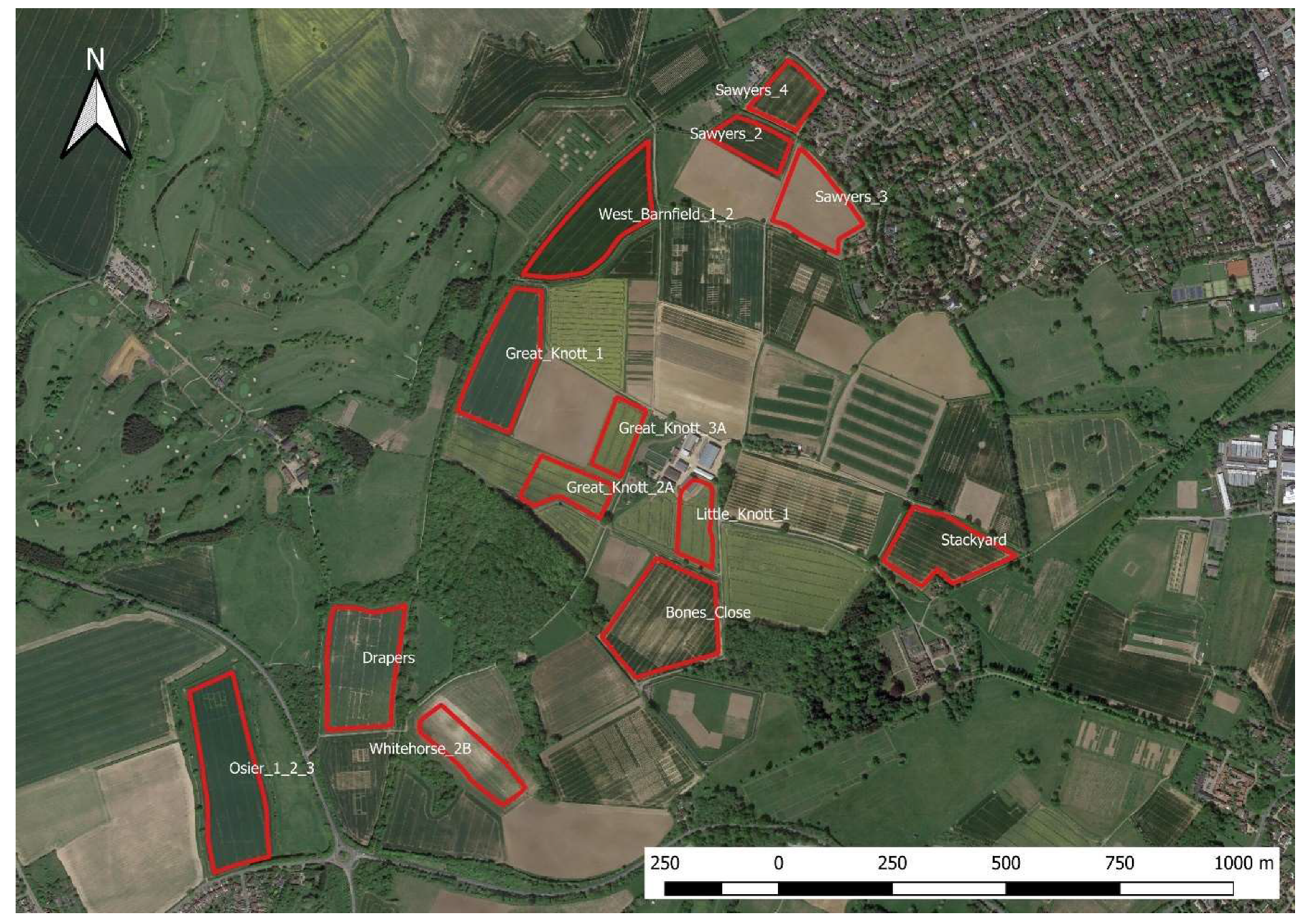
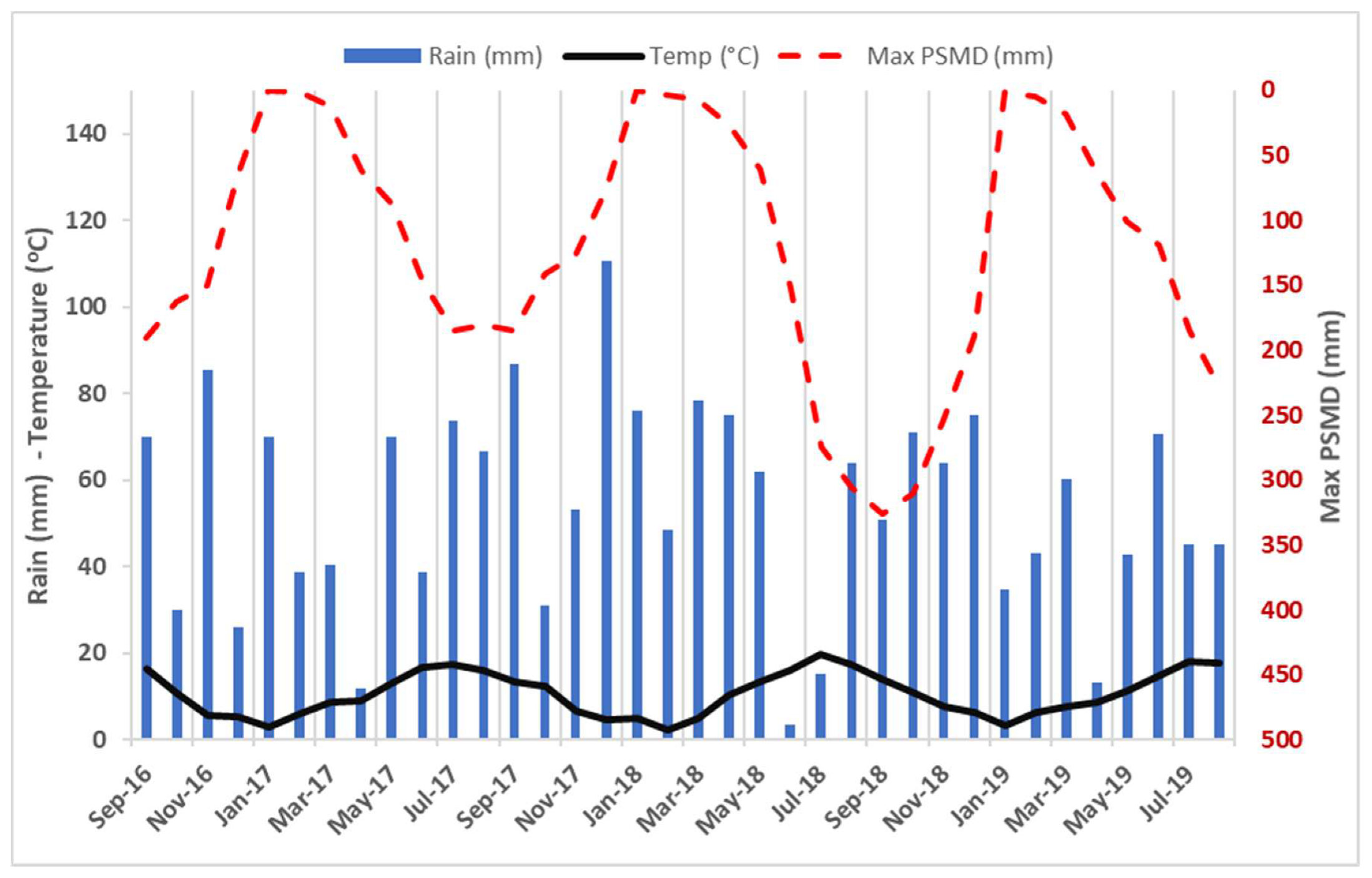
In total, 18 winter wheat fields were selected for the analysis of S1 backscatter interaction with vegetation during the 2017 to 2019 agronomic seasons (nine fields were selected in 2017, five fields in 2018, and four fields in 2019 (Figure 1,

Table 1. Wheat field names and number of 10 × 10 m pixels per field on Rothamsted farm.

Field Name	No. S1 Pixels in Field	Perimeter (m)	Area (ha)	Ground Data Collected
Great_Knott_1	333	805	3.37	2017
Great_Knott_2A	146	555	1.46	2017
Great_Knott_3A	112	457	1.12	2017
Little_Knott_1	122	482	1.22	2017
Osier_1_2_3	479	1046	4.75	2017
Sawyers_3	228	645	2.27	2017, 2019
Whitehorse_2B	191	649	1.90	2017, 2019
Bones_Close	437	810	4.39	2018
Sawyers_2	116	469	1.16	2018
Sawyers_4	131	465	1.30	2017, 2018
Stackyard	276	739	2.77	2017, 2018
West_Barnfield_1_2	365	910	3.62	2018, 2019
Drapers	399	839	3.93	2019

). The fields belong to the Rothamsted Research experimental farm in Harpenden, UK (51°48′37.3″ N, 0°22′36.0″ W), located 35 km north of London (Figure 1). The site comprises slightly acid loamy and clayey soils with restricted drainage [46], and the main soil series at Rothamsted is the Batcombe series [47]. The annual rainfall at the site ranged from 662 mm in 2017 to 704 mm in 2018, and 616 mm in 2019. June and July 2018 were particularly dry [48] and the potential soil moisture deficit (PSMD) reached a maximum value of almost 325 mm. The mean annual air temperature was 10.6 °C, ranging from 2.2 °C in February to 19.9 °C in July (Figure 2).

2.2. Site Ground Measurements of Wheat Development and Yield

In situ observations of phenology were made weekly during the growing season to monitor the wheat development and growth stages. In each field, measurements of grain yield were recorded by the harvest machinery. These data were used as reference points in the methodology to describe the response of the VH/VV ratio to the dynamics of the winter wheat development and growth, and explore the different parameters of the segments with respect to their contribution to yield.

2.3. SAR Data to Obtain VH/VV Time Series in Each Wheat Field

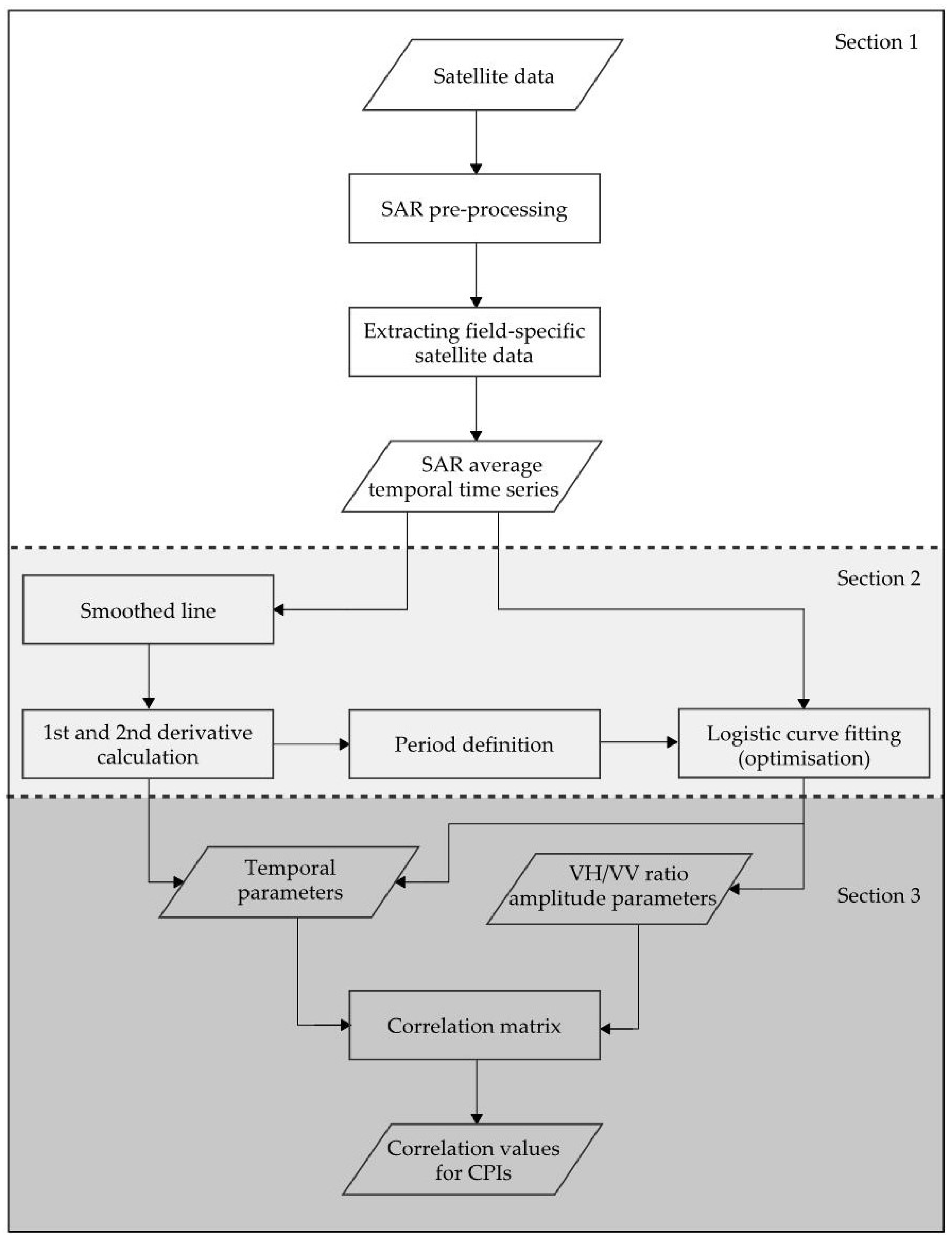
The Sentinel-1 SAR data acquired for the Rothamsted Research farm, over the three-year study period were derived from orbit 132 (ascending) with a temporal resolution of six days. One of the reasons for selecting a single orbit is the orientation of the view of the satellite, which plays a significant role in the direction of the emitted beam from the SAR antenna [49,50]. Using the same orbit also had the advantage of a similar incidence angle (range of 5°) for adjacent fields on even terrain [49]. The ascending orbit 132, instead of descending 81, was also used to avoid early morning measurements when dew may become a confounding factor [14,45]. Temporal profiles of the S1 VH/VV backscatter ratio were plotted on each field to define the curves’ shapes and amplitude, which were related to ground observations of wheat at key growth stages, assisting in the definition of periods defined by the calculated parameters. Figure 3 displays the flow diagram with all the needed steps of the analysis.

2.3.1. SAR Preprocessing for Field Specific VH/VV Time Series

The SAR data were derived from the Level-1 Ground Range Detected Interferometric Wide Swath (GRD-IW) product from Sentinel-1 satellite. The Sentinel-1 toolbox was used to preprocess the data, including border and thermal noise removal, slice assembly, radiometric calibration, terrain flattening, speckle filtering using refined Lee filter with a 3 × 3 window, and terrain correction to produce gamma naught (γ°) data in VH and VV polarisations. Lastly, each scene was clipped and the γ° VH/VV ratio was calculated. Based on the scale selected for the analysis, a mean value for the whole field (Table 1) was used to minimise the speckle effect, and the area of each field was buffered to minimise the influence of surrounding fields. All of the calculations were conducted using untransformed data in a linear form. In the presentation of the results, the initial graphs were developed to allow the reading of both linear and decibel (dB) values, and the final results were presented on decibel axes. In addition, temporal filtering (in the form of smoothing, Savitzky–Golay filter) was used to reduce localised weather patterns, such as heavy rainfall, ice or snow, that can temporarily lower the SAR backscatter. This step avoided the use of additional data (e.g., rainfall used to clean the data) for automation.

2.3.2. Temporal Analysis and Wheat Development Definition

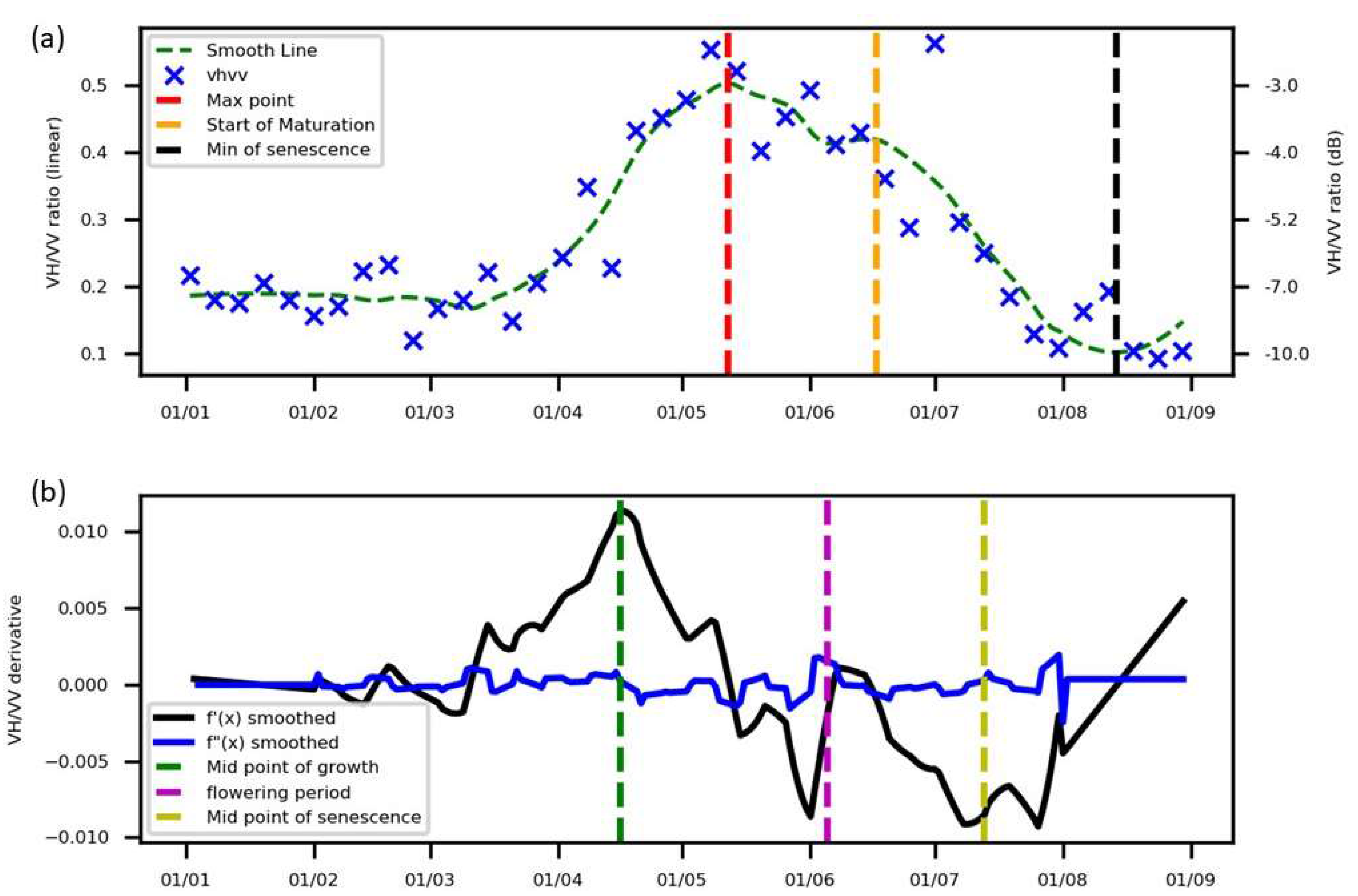
The curve of the VH/VV ratio time series was used to produce indicators that could describe wheat crop growth and development across the season. Smoothing approaches for time series of SAR [51,52] and optical data [42,53] have been used in various studies to reduce noise or fill the gaps of the datasets. Here, the Savitzky–Golay filter was applied over the whole period with a moving window of two months and using a second-order polynomial function [54]. Then the associated first and second derivatives were calculated to define additional wheat growth stages, linked to the SAR temporal characteristics. Key periods of these three curves were identified, as shown as vertical lines in Figure 4, and matched with crop development observed in the field.

The next stage was to further parameterise and automate the extraction of these dates and test if they were linked to wheat development. The smoothed VH/VV curve was divided into two periods: (i) growth and (ii) maturation and senescence to address an observed change in maximum values in the middle of the season. The splitting of the analysis into two periods was also used by Che et al. (2014) [41], who analysed the temporal evolution of the leaf area index (LAI) of vegetation during development and senescence in Shandong Province, China. The breakpoint of two curves occurs during the flowering period (anthesis) when the wheat has reached its full height. The calculation of the breakpoint specifies the start for the VH/VV ratio stabilisation period close to the end of spring.

2.3.3. Logistic Curve Fitting

In order to quantify the characteristics of the temporal curve of VH/VV ratio for winter wheat, a logistic model was used during both the growth and maturation phases. Two separate curves, rather than a single double logistic curve, were chosen because the starting value of the VH/VV ratio of the maturation phase (which coincided with flowering) tended to be lower than the finishing point of the growth stage (which coincided with booting) (Figure 5). In addition, the baseline at the beginning of the season can differ from the end. The two sigmoid logistic curves describing the VH/VV ratio in relation to time t for each stage was characterised by four parameters (Equation (1)):

$$f\left(t\right)=base+\frac{Max}{1+e^{-b\left(t-t_0\right)}}$$

(1)

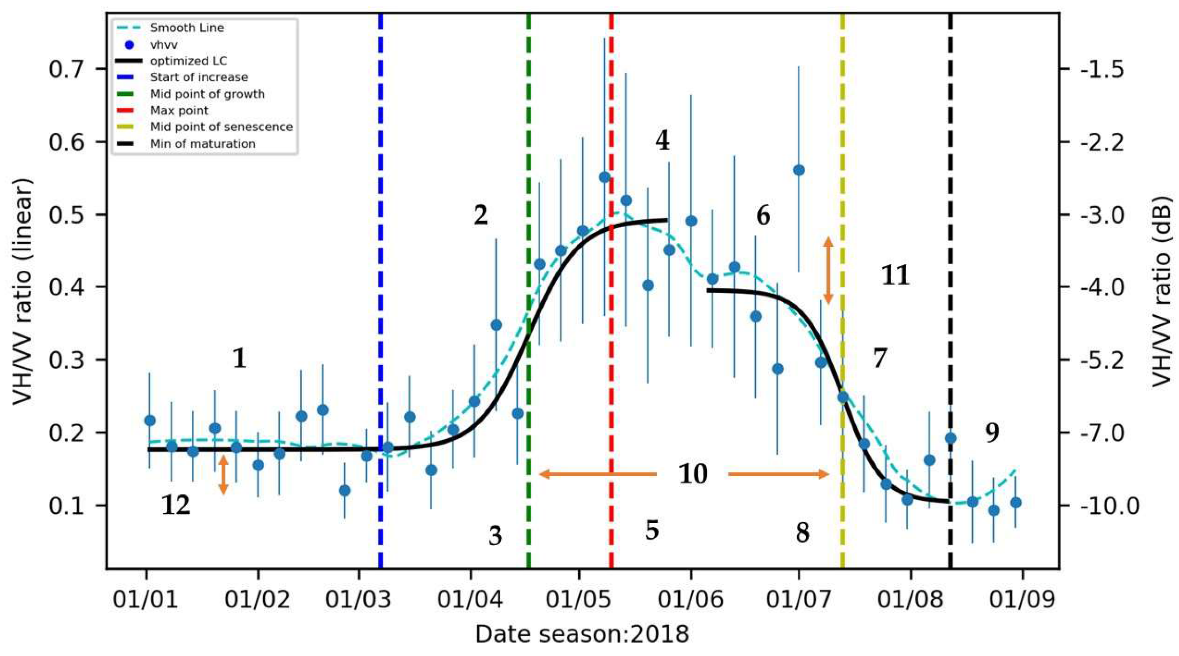
where base is the minimum VH/VV ratio value, Max is the maximum VH/VV ratio value, b is the steepness of the logistic curve, and t_o is the x-value of the sigmoid inflexion point. The calculated values are sensitive to a clear definition of the period represented by each sigmoid curve (Figure 5). The growth period curve was defined from the beginning of the season (Parameter 1 in Figure 5) up to the time of maximum value of the smoothed curve (Parameter 5). The maturation period curve was defined as the period after flowering to the minimum value in the maturation period of the temporally smoothed curve.

Combining parameters extracted from the two logistic curves allowed us to derive three additional vegetation development-related parameters (10, 11, and 12 in Figure 5). The period between the two midpoints of the logistic curves (Parameter 10 in Figure 5) was defined as the duration of “full” vegetation, which starts with stem elongation and ends with the reduction of the green canopy and translocation of carbohydrates into the grain during maturation. The difference in baselines is related to the backscatter from the biomass of the crop during tillering. The summary of the extracted parameters and their definitions as well as the associated crop development stage is given in

Table 2. Definitions of the VH/VV ratio curve parameters and the anticipated associated crop development stage (Biologische Bundesanstalt, Bundessortenamt und CHemische Industrie - BBCH or Zadoks scale).

No.	Symbol	Parameter Name	Definition	Derived From	Associated Crop Development Stage
1	G_base	Baseline value for the growth stage	VH/VV ratio at the beginning of the season	Logistic curve	Tillering (GS20)
2	G_steep	Steepness of logistic curve for growth period	Rate of coefficient in Equation (1) (b G)	Logistic curve	Stem elongation
3	G_midP	Time of midpoint of growth period (t0, G)	DOY when the midpoint of the logistic curve occurs in the growth period	Logistic curve	Stem elongation
4	G_max	Max value for growth stage	Maximum VH/VV ratio value for the full season	Logistic curve	End of stem elongation (GS39) and booting (GS49)
5	TZmax	Time of maximum point	DOY of maximum smoothed value of VH/VV	Smoothed curve	Time of booting, flag leaf unrolled
6	S_max	Value at the start of grain filling	Period of backscatter stabilisation	Logistic curve	Post anthesis: start of grain filling (GS71)
7	S_steep	Steepness of logistic curve for maturation period	Rate of coefficient in Equation (1) (b S)	Logistic curve	Maturation rate
8	S_midP	Time of midpoint of maturation (t0, S)	DOY when the midpoint of the logistic curve occurs in the maturation period	Logistic curve	Ripening (GS 85–89)
9	S_base	Baseline value at the end of the season	Background value of the VH/VV ratio	Logistic curve	After harvestPeriod with soil exposed
10	Duration	Duration of “full” vegetation to maturation	Time difference between midpoints (3, 8)	Combination	Period of most of the photosynthate accumulation and translocation
11	D_max	Structure change (Inflorescence)	VH/VV ratio value differences between booting and grain filling periods (4–6)	Combination	Backscatter change during the period when the ear emerges
12	D_base	Tillering backscatter	VH/VV ratio value differences between tillering and bare soil (1–9)	Combination	Tillering with reduced impact of soil

.

2.3.4. Parameter Optimisation

The calculation of the logistic curve fitting parameters in Table 2 was based on a weighted least squares (WLS) estimator, which considers the uncertainty of each point by minimising the sum of the squared difference divided by the respective standard deviation (σ) in each point (Equation (2)). The incorporation of the standard deviation in the estimator was used to minimise the outlier effects. The VH/VV ratio points were selected as the observation values in each defined period.

$$min{\displaystyle \sum }_i{\left(\frac{ob{s}_i-y_i}{{\sigma }_{\iota }}\right)}^2$$

(2)

2.3.5. Automatic Curve Extraction and Correlation Analysis

By scripting the SAR processing using Python, it was possible to automatically derive a smoothed VH/VV ratio curve and two logistic curves. Then the 12 parameters were derived for each field site across three years. A Pearson correlation coefficient (r) was calculated for each pair in a matrix. This approach allows the illustration of the interactions between the parameters and the direct effect on final crop yield. A significant test of the r was performed and highlighted in the plots.

3. Results

3.1. Annual Analysis of VH/VV Ratio Curve Parameters, 2017 to 2019

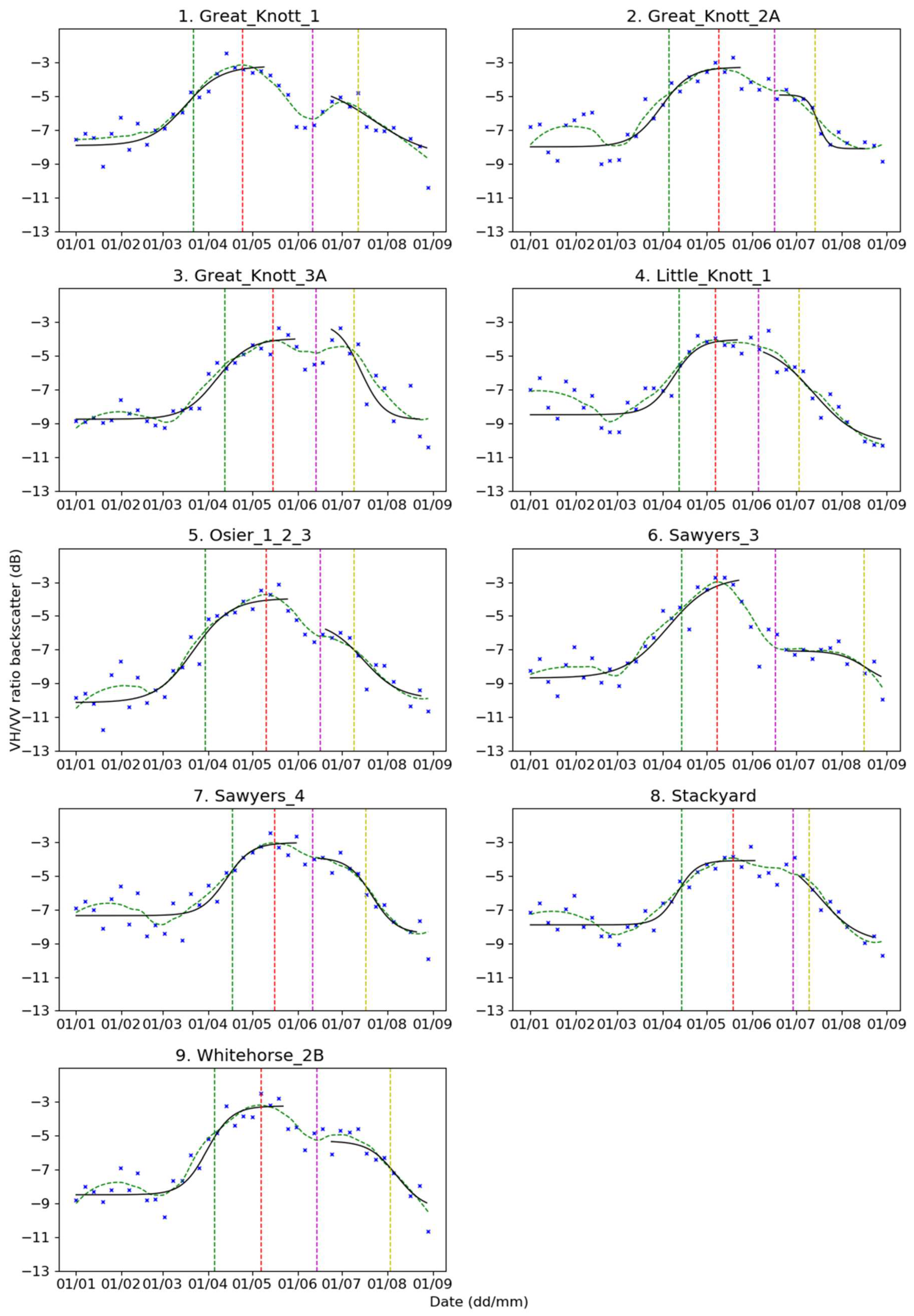
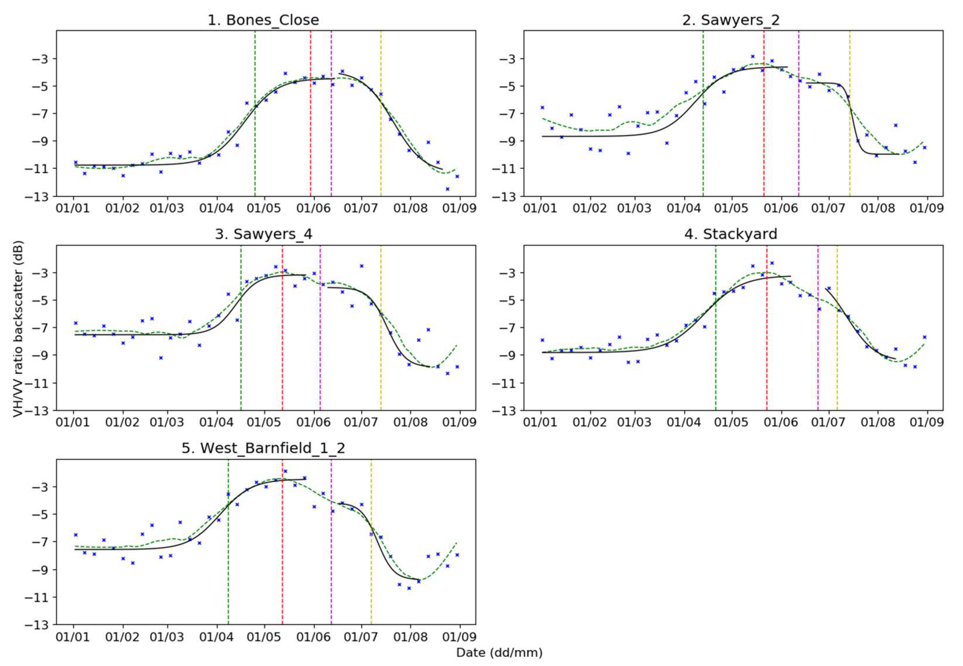
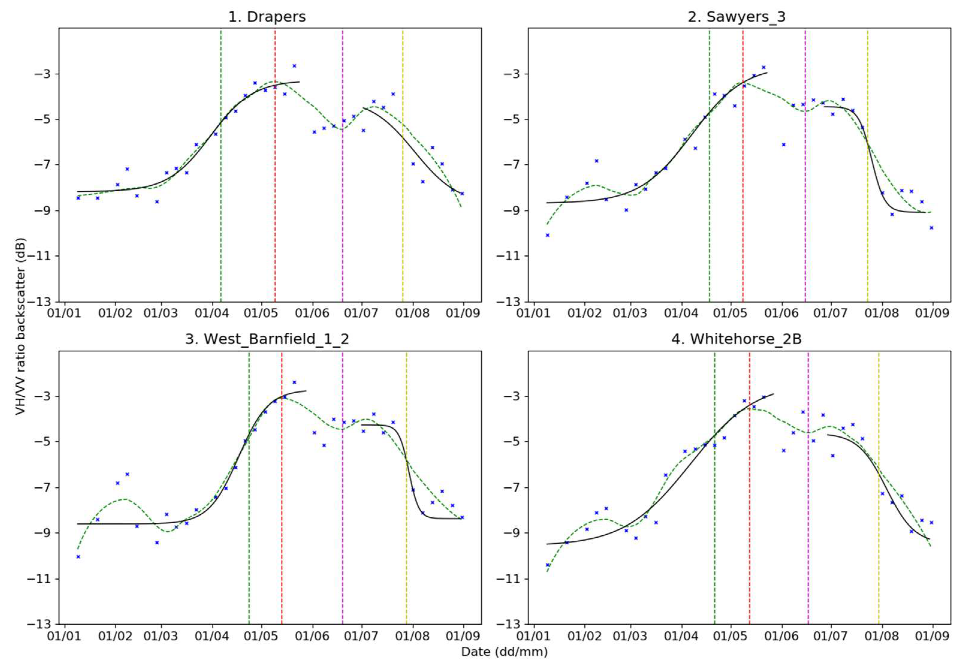
Two logistic curves for the nine fields selected in 2017 (Figure 6), the five fields selected in 2018 (Figure 7), and the four fields selected in 2019 (Figure 8), were plotted. The smoothed time series were used to identify the start and end of (i) the growth (start of the year to red line) and (ii) the maturation periods (purple to min senescence value). Then the midpoints were calculated by fitting the logistic curves in these periods, creating the time parameters shown in Figure 6, Figure 7 and Figure 8.

The timing of the mean maximum VH/VV ratio (TZ_max) was relatively consistent varying from day-of-year (DOY) 129 in 2017, to DOY 140 in 2018, and DOY 131 in 2019 (

Table 3. Values of derived parameters (linear scale), yield data, and the root mean standard error of the growth (RMSE_G) and maturation (RMSE_S) stages, for each of the winter wheat fields in 2017, 2018, and 2019. Note: day-of-year, DOY.

Field	Season	RMSEG	RMSES	G_base	G_steep	G_max	S_max	S_steep	S_base	G_midP	S_midP	TZmax	Duration	D_max	D_base	Yield
										DOY	DOY	DOY	days			t/ha
Great_Knott_1	2017	0.051	0.004	0.16	0.077	0.36	0.25	−0.05	0.14	85	194	114	109	0.11	0.020	8.67
Great_Knott_2A	2017	0.092	0.022	0.16	0.115	0.28	0.17	−0.29	0.15	93	196	129	103	0.12	0.010	6.43
Great_Knott_3A	2017	0.020	0.047	0.13	0.11	0.24	0.37	−0.13	0.13	99	190	135	91	−0.13	0.000	9.26
Little_Knott_1	2017	0.090	0.033	0.14	0.108	0.31	0.28	−0.07	0.10	106	184	127	78	0.02	0.040	6.17
Osier_1_2_3	2017	0.054	0.004	0.10	0.072	0.34	0.20	−0.08	0.10	93	190	130	97	0.14	0.000	6.63
Sawyers_3	2017	0.070	0.012	0.14	0.066	0.45	0.07	−0.11	0.12	108	228	128	120	0.38	0.020	6.36
Sawyers_4	2017	0.047	0.004	0.18	0.115	0.33	0.26	−0.12	0.14	108	199	136	90	0.07	0.040	6.85
Stackyard	2017	0.037	0.002	0.16	0.159	0.22	0.30	−0.08	0.13	103	191	139	88	−0.08	0.030	5.04
Whitehorse_2B	2017	0.061	0.035	0.14	0.143	0.30	0.18	−0.11	0.11	93	215	127	122	0.12	0.030	9.59
Bones_Close	2018	0.021	0.017	0.08	0.098	0.28	0.33	−0.11	0.07	117	194	150	78	−0.05	0.010	4.09
Sawyers_2	2018	0.118	0.035	0.13	0.102	0.31	0.23	−0.45	0.10	104	196	141	91	0.08	0.030	6.58
Sawyers_4	2018	0.051	0.069	0.18	0.12	0.40	0.29	−0.18	0.10	111	195	132	84	0.11	0.080	5.49
Stackyard	2018	0.044	0.009	0.13	0.071	0.49	0.39	−0.12	0.11	121	187	143	66	0.10	0.020	4.81
W_Barnfield_1_2	2018	0.057	0.012	0.17	0.094	0.43	0.28	−0.20	0.11	101	189	132	88	0.15	0.060	7.90
Drapers	2019	0.018	0.047	0.15	0.079	0.32	0.26	−0.08	0.13	97	207	129	110	0.06	0.018	9.65
Sawyers_3	2019	0.007	0.026	0.14	0.065	0.41	0.24	−0.26	0.12	108	205	128	97	0.17	0.012	7.99
W_Barnfield_1_2	2019	0.030	0.036	0.14	0.114	0.40	0.23	−0.34	0.15	113	209	133	96	0.17	−0.008	8.28
Whitehorse_2B	2019	0.021	0.029	0.11	0.053	0.47	0.23	−0.12	0.11	112	211	132	99	0.23	−0.002	10.17

). The mean values (

Table 4. Mean and standard deviation values of 12 derived parameters (linear scale) and the wheat yield for each season of the analysis.

Season		G_base	G_steep	G_max	S_max	S_steep	S_base	G_midP	S_midP	TZmax	Duration	D_max	D_base	Yield
								DOY	DOY	DOY	days			t/ha
2017	Mean	0.15	0.11	0.31	0.23	−0.12	0.12	99	199	129	100	0.08	0.02	7.22
	Std dev	0.02	0.03	0.07	0.09	0.07	0.02	8	14	7	15	0.14	0.02	1.56
2018	Mean	0.14	0.10	0.38	0.30	−0.21	0.10	111	192	140	81	0.08	0.04	5.77
	Std dev	0.04	0.02	0.09	0.06	0.14	0.02	8	4	8	10	0.08	0.03	1.50
2019	Mean	0.13	0.08	0.40	0.24	−0.20	0.13	107	208	131	101	0.16	0.01	9.02
	Std dev	0.02	0.03	0.06	0.01	0.12	0.01	7	3	2	7	0.07	0.01	1.00

) of the three parameters of the logistic curve for the growth period were also relatively consistent from year to year: G_base (range 0.13–0.15), G_steep (range: 0.08–0.11), and G_midP (range: DOY 99 to 109). There was greater variation in G_max, which ranged from a mean of 0.31 in 2017 to 0.40 in 2019. The mean values of two of the parameters of the logistic curve for the maturation period were also relatively similar across the three years: S_base (range: 0.10–0.13), and S_midP (range: DOY 199 to DOY 208). By contrast, the mean values of S_max (range: 0.23–0.30) and S_steep (range: –0.12 to –0.21) showed greater interannual variation (Table 4).

The root mean square error (RMSE) of the growth (G) and maturation (S) logistic curves are shown in the last two columns of Table 3 for the seasons 2017, 2018, and 2019. Statistical comparison between the parameters of different years showed that TZmax (p = 0.042), the G_midP (p = 0.037), S_base (p = 0.030) are significantly different at 95% confidence using ANOVA or the Kruskal–Wallis H-test if there was a non-normal distribution. There was also a significant interannual variation in the Duration (p = 0.039) and Yield (p = 0.016).

3.2. Relationship Between SAR-Derived Parameters and Yield

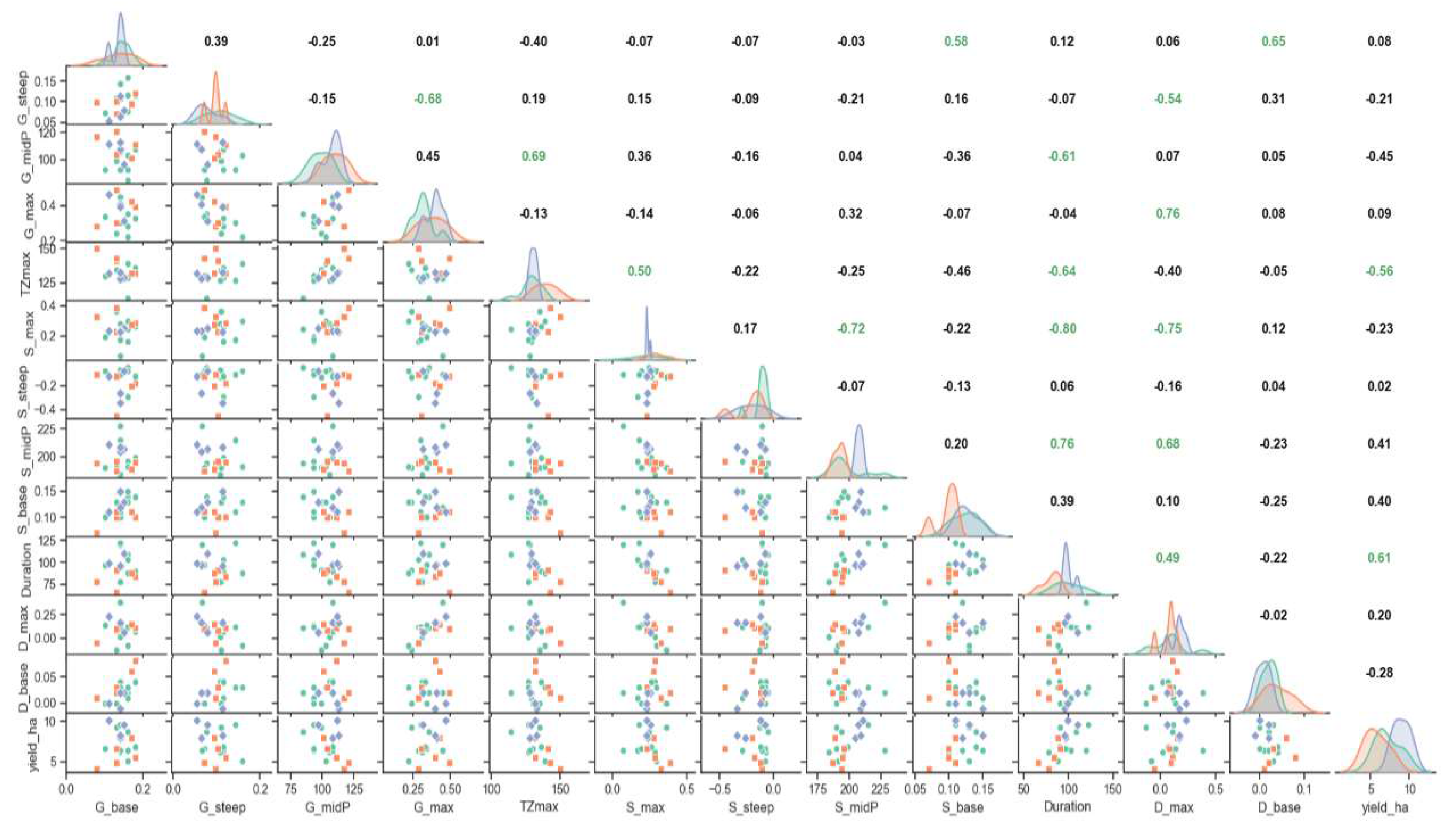
The interactions between each of the parameters and yield were further displayed using a correlation matrix (Figure 9). There were various significant correlations between parameters. As would be expected, the inflorescence indicator (D_max = G_max – S_max) was correlated with the two parameters used in the calculation (G_max and S_max), with r values of 0.76 and −0.75, respectively. At the same time, significant correlations were found between D_max and G_steep (r = −0.54), S_midP (r = 0.68), and Duration (r = 0.49). By contrast, D_base displayed no significant correlations with the other parameters, with the exception of G_base (r = 0.65) that was used for its calculation. The definition of D_base is G_base minus S_base, where S_base represents the VH/VV ratio value on bare soil (that should remain relatively consistent) and the value of G_base is determined by the combination of soil and low vegetation during the tillering period.

Starting from the first row in Figure 9, the baseline of growth (G_base) shows a significant positive correlation (r = 0.58) with the baseline of maturation (S_base). This is because G_base depends on the shift of the VH/VV ratio during the initial bare/sparse/small vegetation period and the soil background (S_base). In the second row, the slope of the midpoint of growth (G_steep) has a negative correlation with the VH/VV ratio at G_max value (r = −0.68). In the third row, the midpoint of growth (G_midP) is highly correlated with the timing of the max (TZmax) smoothed VH/VV ratio value (r = 0.69), highlighting the interaction of stem elongation and booting stage. G_midP was also correlated with the calculated Duration (r = −0.68) and the maturation midpoint (S_midP; r = 0.78). This is because the Duration value is defined by the difference between these two time indicators. The value of TZmax, the timing of the maximum value of VH/VV, was positively correlated with S_max (r = 0.50), but negatively correlated with low Duration values (r = −0.64).

During the maturation period, S_max was negatively correlated with the midpoint S_midP (r = −0.72) and Duration (r = −0.80). The only correlation shown by the steepness of the curve in this period was with the yield. The value of S_midP was positively correlated with Duration (r = 0.76) and D_max (r = 0.68). The value of S_base was not significantly correlated with any of the indicators except G-base.

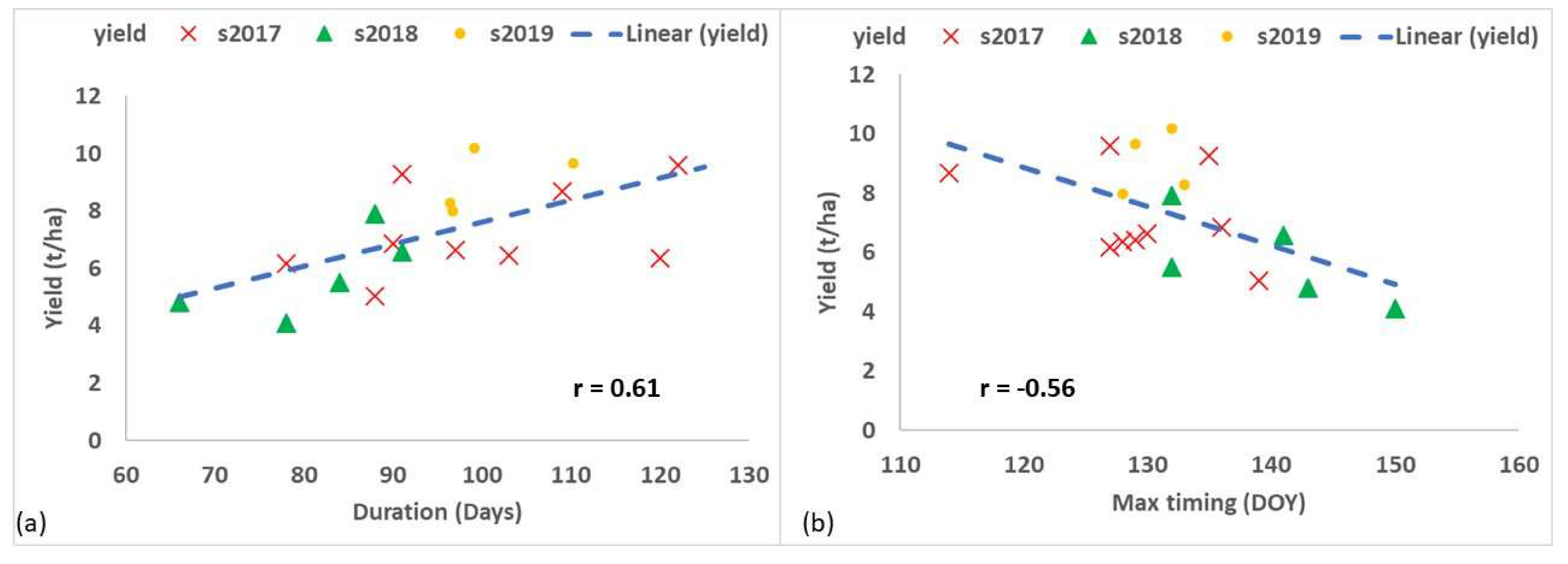
As illustrated by the matrix (Figure 9), multiple correlations exist among the individual parameters and between individual parameters and yield (last column). The results suggest that the two parameters, G_midP and TZmax (which are correlated), had the strongest association with grain yield, i.e., r = −0.45 and r = −0.56, respectively, after Duration (r = 0.61). The negative correlation suggests that earlier growth, i.e., lower values of G_midP and TZmax were associated with higher end-of-season grain yields. Figure 10 displays the two most significant parameters that are sensitive to yield.

4. Discussion

Using the example of winter wheat over three growing seasons, it was possible to derive field-specific annual coefficients of a generalised two-component empirical model of crop productivity from the SAR VH/VV ratio. Due to the ubiquitous and high-frequency availability of S1 data, this approach could offer new opportunities for monitoring and predicting productivity in areas affected by frequent cloud cover. The characterisation of VH/VV response over a season used three stages: (i) the creation of a smooth VH/VV time series for each field; (ii) the definition of the timing of the maximum value using temporal characteristics of the time series, growth, and maturation period using first and second derivatives; and (iii) the creation of two logistic curves using the observation in the predefined periods of growth and maturation [41]. The results are discussed as follows: first, in terms of the robustness of our mathematical method over three seasons to consider multiple factors of variation; second, the gain of biophysical understanding using this method; and finally, the agronomic potential of our results.

4.1. Technical and Statistical Process, the Goodness of Fit, Robustness, and Uncertainty

Since 2016, SAR data from Sentinel-1 have become twice as frequent as data used in previous studies [2,20], which improves the robustness of the possible analysis. However, to reduce the variability of SAR data we chose to use imagery from only the ascending satellite passing as images from the descending orbit were often affected by morning dew. Similar observations have been made in other studies [14,45], indicating greater certainty when using the ascending rather the descending phase of the satellite for predicting crop state variables in this area. Even so, the results demonstrate substantial variation of SAR backscatter, which can be due to differences in topography affecting the incidence angle or changes in canopy architecture [49,50].

As pointed out in an earlier review [5], SAR variability is also connected to diurnal variation in plant–soil–water relations, which can affect the erectness of the crop canopy and the dielectric properties of the system. To reduce the effect of such fluctuations in the SAR time series, our approach used a step of smoothing the data, which resulted in a set of relatively consistent dynamic curves for winter cereals [20], and limited the extreme values of the VH/VV (Figure 6). The subsequent logistic fitting approach enabled the calculation of a specific backscatter value and time-specific parameters from the VH/VV ratio data (Figure 5). Accounting for the standard deviation during the fitting of the logistic curves made it possible to give lower weight to data with high uncertainty and improved the precision of the derived curves. The average RMSE values of the logistic curve fitting in growth (G) and senescence/maturation (S) periods were 0.05 and 0.07, respectively.

The creation of the fitted curves allowed the derivation of 12 parameters that can be related to the development, growth, and yield of winter wheat. Two temporal parameters from the analysis (TZmax and Duration) were significantly correlated with yield (Figure 9). Further analysis could focus on the opportunity of using a combination of parameters or a combination of VV and VH/VV values. The approach was effective in each of three years that were characterised by different environmental conditions and yields. In 2018, there was minimal rainfall in June and July, and the grain yields obtained in 2018 (4.09–7.01 t ha⁻¹) were substantially lower than in 2017 (5.04–9.59 t ha⁻¹) and 2019 (7.99–10.17 t ha⁻¹).

4.2. Environmental and Biophysical Understanding

The sensitivity of SAR backscatter to surface changes in the structure and the soil and crop water content means that SAR can be an effective tool to monitor crop development [5,24] starting from early growth, to the increase in the water volume of the crop through stem elongation, and its decrease during maturity. In this paper, we assigned two separate logistic curves during the cropping season to examine whether the resulting parameters were correlated with observations in the field. A specific feature of creating two curves is the derivation of the D_max value, which would not be captured by assuming a single curve. Our interpretation is that the change in the VH/VV value at flowering is a real effect, which equates to a change in the structure of the crop (Figure 6) during the inflorescence period, as mentioned by other authors [2,14,18]. Even so, the value of D_max was variable, ranging from –0.13 to 0.38 for an individual field and year (Table 3). Additional research, including perhaps data focused on structure, is required to further understand this variability.

The correlation analysis (Figure 9) was able to identify two time-based parameters, one derived from the growth period (G_midP) and one derived from the smoothed VH/VV curve (TZmax), which were negatively associated with the final grain yield (r = −0.45 and −0.56, respectively). This means that a delayed occurrence of the midpoint of the growth curve and the timing of the maximum VH/VV ratio was associated with lower grain yields. The late or slow growth of the crop canopy is likely to result in a reduced capacity of the crop to intercept solar radiation and use photosynthesis to produce assimilates required for final yield. For example, in 2018, the late occurrence of G_midP and TZmax was associated with an unusually dry period in June and July 2018 (Figure 2), which reduced canopy growth and photosynthesis and resulted in substantially lower grain yields than in the other two years.

The analysis also showed that the duration of the period of “full” vegetation (Duration) was positively related to grain yield (r = 0.61). This can be explained by the yield benefitting from a longer period of photosynthesis and a longer grain-filling period when assimilates are transferred from green tissue to the grain [55,56]. These results suggest that using the VH/VV ratio to identify the timing of specific crop periods, which are related to the structural change of the wheat canopy [2,14], may be a more useful determinant of yield than the actual values of the VH/VV ratio, per se.

4.3. Opportunities for Agronomic Management and Modelling

The analysis raises two questions for crop management. First, what can be learnt about crop dynamics from monitoring satellite-based SAR data, dynamics, and amplitude? Second, is there potential for a farmer or agronomist to use SAR-derived indicators for spatially varying crop management and inputs between fields? The growth and development of a wheat crop depends on the interaction between the weather (e.g., solar radiation, rainfall, and temperature), crop genetics, field characteristics (e.g., aspect and soil type), and field management (e.g., previous cropping history and the timing, type of cultivation, and drilling). The results from the SAR data analysis indicates that it is possible to identify seasonal differences in the timing of crop growth, and this may be useful in identifying the most appropriate schedule of fertilizer and agrochemical application between fields. The analysis also suggests that it may be possible to improve the prediction of the eventual crop yield from an analysis of SAR characteristics.

A potential limitation with the method is that some of the parameters are determined retrospectively from a full temporal dataset, for example, the calculation of TZmax, the timing of the maximum value of VV/VH, requires data that occur after TZmax. Likewise, the value of S_steep, which occurs during the maturation of the crop, requires data that occur after that point. Developing a really effective predictive tool that can be used to modify field management instantaneously will require parameters that can be estimated in real-time. Further work is needed to improve the estimation of parameters, as well as the application of the methodology on other farms to validate the robustness of the method. The correlation of the productivity indicators with field measurements also has the potential to assist in better model simulations of crop development and growth. At the same time, temporal characteristics, as well as connection with the biophysical properties of the field, could be examined to improve the calibration and its incorporation into a data assimilation framework to estimate more efficiently the field production [1,7,8].

5. Conclusions

This paper describes a new methodology to derive wheat productivity indicators from Sentinel-1 VH/VV time series. The temporal curves, their first and second derivatives, and logistic curve fitting for growth and maturation periods were used to define 12 phenomorphological parameters. These provide information about the growth, development, and yield of wheat crop at field scale, offering an alternative approach to ground survey or yield estimation.

The analysis of the VH/VV ratio time series and the correlation matrix indicates that the time-based parameters appear to be related to biophysical changes in the field. In particular, the time period of “full” vegetation (Duration) was positively correlated with yield (r = 0.61), and a delay in the timing of the maximum VH/VV value (TZmax) was negatively correlated with yield (r = −0.56).

Automation of the SAR image analysis was possible, as the only inputs required were backscatter data from VH and VV polarisations. Future work will explore the use of this method to estimate commercial wheat production in other farming landscapes in the UK. It could also be adapted to monitor growth and development, as well as yield prediction for other arable crops, potentially allowing the remote quantitative assessment of environment and management impacts.

References

- Jin, X.; Kumar, L.; Li, Z.; Feng, H.; Xu, X.; Yang, G.; Wang, J. A review of data assimilation of remote sensing and crop models. Eur. J. Agron. 2018, 92, 141–152. [Google Scholar] [CrossRef]
- Veloso, A.; Mermoz, S.; Bouvet, A.; Le Toan, T.; Planells, M.; Dejoux, J.-F.; Ceschia, E. Understanding the temporal behavior of crops using Sentinel-1 and Sentinel-2-like data for agricultural applications. Remote Sens. Environ. 2017, 199, 415–426. [Google Scholar] [CrossRef]
- De Sy, V.; Herold, M.; Achard, F.; Asner, G.P.; Held, A.; Kellndorfer, J.; Verbesselt, J. Synergies of multiple remote sensing data sources for REDD+ monitoring. Curr. Opin. Environ. Sustain. 2012, 4, 696–706. [Google Scholar] [CrossRef]
- Kansakar, P.; Hossain, F. A review of applications of satellite earth observation data for global societal benefit and stewardship of planet earth. Space Policy 2016, 36, 46–54. [Google Scholar] [CrossRef]
- Steele-Dunne, S.C.; McNairn, H.; Monsivais-Huertero, A.; Judge, J.; Liu, P.-W.; Papathanassiou, K. Radar Remote Sensing of Agricultural Canopies: A Review. IEEE J. Sel. Top. Appl. Earth Obs. Remote Sens. 2017, 10, 2249–2273. [Google Scholar] [CrossRef] [Green Version]
- Kasampalis, D.; Alexandridis, T.; Deva, C.; Challinor, A.; Moshou, D.; Zalidis, G. Contribution of Remote Sensing on Crop Models: A Review. J. Imaging 2018, 4, 52. [Google Scholar] [CrossRef] [Green Version]
- Betbeder, J.; Fieuzal, R.; Baup, F. Assimilation of LAI and Dry Biomass Data From Optical and SAR Images Into an Agro-Meteorological Model to Estimate Soybean Yield. IEEE J. Sel. Top. Appl. Earth Obs. Remote Sens. 2016, 9, 2540–2553. [Google Scholar] [CrossRef]
- Huang, J.; Gómez-Dans, J.L.; Huang, H.; Ma, H.; Wu, Q.; Lewis, P.E.; Liang, S.; Chen, Z.; Xue, J.H.; Wu, Y.; et al. Assimilation of remote sensing into crop growth models: Current status and perspectives. Agric. For. Meteorol. 2019, 276, 107609. [Google Scholar] [CrossRef]
- Blaes, X.; Defourny, P.; Wegmuller, U.; Della Vecchia, A.; Guerriero, L.; Ferrazzoli, P. C-band polarimetric indexes for maize monitoring based on a validated radiative transfer model. IEEE Trans. Geosci. Remote Sens. 2006, 44, 791–800. [Google Scholar] [CrossRef]
- Casanova, J.J.; Judge, J.; Jang, M. Modeling Transmission of Microwaves Through Dynamic Vegetation. IEEE Trans. Geosci. Remote Sens. 2007, 45, 3145–3149. [Google Scholar] [CrossRef]
- Van Emmerik, T.; Steele-Dunne, S.C.; Judge, J.; van de Giesen, N. Impact of Diurnal Variation in Vegetation Water Content on Radar Backscatter From Maize During Water Stress. IEEE Trans. Geosci. Remote Sens. 2015, 53, 3855–3869. [Google Scholar] [CrossRef]
- Vicente-Guijalba, F.; Martinez-Marin, T.; Lopez-Sanchez, J.M. Crop Phenology Estimation Using a Multitemporal Model and a Kalman Filtering Strategy. IEEE Geosci. Remote Sens. Lett. 2014, 11, 1081–1085. [Google Scholar] [CrossRef] [Green Version]
- Aschbacher, J.; Milagro-Pérez, M.P. The European Earth monitoring (GMES) programme: Status and perspectives. Remote Sens. Environ. 2012, 120, 3–8. [Google Scholar] [CrossRef]
- Harfenmeister, K.; Spengler, D.; Weltzien, C. Analyzing Temporal and Spatial Characteristics of Crop Parameters Using Sentinel-1 Backscatter Data. Remote Sens. 2019, 11, 1569. [Google Scholar] [CrossRef] [Green Version]
- Friesen, J.; Steele-Dunne, S.C.; van de Giesen, N. Diurnal Differences in Global ERS Scatterometer Backscatter Observations of the Land Surface. IEEE Trans. Geosci. Remote Sens. 2012, 50, 2595–2602. [Google Scholar] [CrossRef]
- Paget, A.C.; Long, D.G.; Madsen, N.M. RapidScat Diurnal Cycles Over Land. IEEE Trans. Geosci. Remote Sens. 2016, 54, 3336–3344. [Google Scholar] [CrossRef]
- Ndikumana, E.; Ho Tong Minh, D.; Dang Nguyen, H.; Baghdadi, N.; Courault, D.; Hossard, L.; El Moussawi, I. Estimation of Rice Height and Biomass Using Multitemporal SAR Sentinel-1 for Camargue, Southern France. Remote Sens. 2018, 10, 1394. [Google Scholar] [CrossRef] [Green Version]
- Mattia, F.; Le Toan, T.; Picard, G.; Posa, F.I.; D’Alessio, A.; Notarnicola, C.; Gatti, A.M.; Rinaldi, M.; Satalino, G.; Pasquariello, G. Multitemporal c-band radar measurements on wheat fields. IEEE Trans. Geosci. Remote Sens. 2003, 41, 1551–1560. [Google Scholar] [CrossRef]
- Alexakis, D.D.; Mexis, F.D.K.; Vozinaki, A.E.K.; Daliakopoulos, I.N.; Tsanis, I.K. Soil Moisture Content Estimation Based on Sentinel-1 and Auxiliary Earth Observation Products. A Hydrological Approach. Sensors 2017, 17, 1455. [Google Scholar] [CrossRef] [Green Version]
- Vreugdenhil, M.; Wagner, W.; Bauer-Marschallinger, B.; Pfeil, I.; Teubner, I.; Rüdiger, C.; Strauss, P. Sensitivity of Sentinel-1 Backscatter to Vegetation Dynamics: An Austrian Case Study. Remote Sens. 2018, 10, 1396. [Google Scholar] [CrossRef] [Green Version]
- Dobson, M.; Ulaby, F.; Hallikainen, M.; El-Rayes, M. Microwave Dielectric Behavior of Wet Soil-Part II: Dielectric Mixing Models. IEEE Trans. Geosci. Remote Sens. 1985, GE-23, 35–46. [Google Scholar] [CrossRef]
- Mironov, V.L.; Dobson, M.C.; Kaupp, V.H.; Komarov, S.A.; Kleshchenko, V.N. Generalized refractive mixing dielectric model for moist soils. IEEE Trans. Geosci. Remote Sens. 2004, 42, 773–785. [Google Scholar] [CrossRef]
- Snapir, B.; Waine, T.W.; Corstanje, R.; Redfern, S.; De Silva, J.; Kirui, C. Harvest Monitoring of Kenyan Tea Plantations With X-Band SAR. IEEE J. Sel. Top. Appl. Earth Obs. Remote Sens. 2018, 11, 930–938. [Google Scholar] [CrossRef]
- Bargiel, D. A new method for crop classification combining time series of radar images and crop phenology information. Remote Sens. Environ. 2017, 198, 369–383. [Google Scholar] [CrossRef]
- McNairn, H.; Champagne, C.; Shang, J.; Holmstrom, D.; Reichert, G. Integration of optical and Synthetic Aperture Radar (SAR) imagery for delivering operational annual crop inventories. ISPRS J. Photogramm. Remote Sens. 2009, 64, 434–449. [Google Scholar] [CrossRef]
- Van Tricht, K.; Gobin, A.; Gilliams, S.; Piccard, I. Synergistic use of radar Sentinel-1 and optical Sentinel-2 imagery for crop mapping: A case study for Belgium. Remote Sens. 2018, 10, 1642. [Google Scholar] [CrossRef] [Green Version]
- De Bernardis, C.; Vicente-Guijalba, F.; Martinez-Marin, T.; Lopez-Sanchez, J.M. Contribution to Real-Time Estimation of Crop Phenological States in a Dynamical Framework Based on NDVI Time Series: Data Fusion With SAR and Temperature. IEEE J. Sel. Top. Appl. Earth Obs. Remote Sens. 2016, 9, 3512–3523. [Google Scholar] [CrossRef] [Green Version]
- Fieuzal, R.; Baup, F.; Marais-Sicre, C. Monitoring Wheat and Rapeseed by Using Synchronous Optical and Radar Satellite Data—From Temporal Signatures to Crop Parameters Estimation. Adv. Remote Sens. 2013, 2, 162–180. [Google Scholar] [CrossRef] [Green Version]
- Zhou, T.; Pan, J.; Zhang, P.; Wei, S.; Han, T. Mapping Winter Wheat with Multi-Temporal SAR and Optical Images in an Urban Agricultural Region. Sensors 2017, 17, 1210. [Google Scholar] [CrossRef]
- Gao, Q.; Zribi, M.; Escorihuela, M.; Baghdadi, N.; Segui, P. Irrigation Mapping Using Sentinel-1 Time Series at Field Scale. Remote Sens. 2018, 10, 1495. [Google Scholar] [CrossRef] [Green Version]
- Baghdadi, N.; El Hajj, M.; Zribi, M.; Bousbih, S. Calibration of the Water Cloud Model at C-Band for Winter Crop Fields and Grasslands. Remote Sens. 2017, 9, 969. [Google Scholar] [CrossRef] [Green Version]
- Bériaux, E.; Waldner, F.; Collienne, F.; Bogaert, P.; Defourny, P. Maize Leaf Area Index Retrieval from Synthetic Quad Pol SAR Time Series Using the Water Cloud Model. Remote Sens. 2015, 7, 16204–16225. [Google Scholar] [CrossRef] [Green Version]
- Li, J.; Wang, S. Using SAR-derived vegetation descriptors in a water cloud model to improve soil moisture retrieval. Remote Sens. 2018, 10, 1370. [Google Scholar] [CrossRef] [Green Version]
- Clauss, K.; Ottinger, M.; Leinenkugel, P.; Kuenzer, C. Estimating rice production in the Mekong Delta, Vietnam, utilizing time series of Sentinel-1 SAR data. Int. J. Appl. Earth Obs. Geoinf. 2018, 73, 574–585. [Google Scholar] [CrossRef]
- Mandal, D.; Kumar, V.; Ratha, D.; Dey, S.; Bhattacharya, A.; Lopez-Sanchez, J.M.; McNairn, H.; Rao, Y.S. Dual polarimetric radar vegetation index for crop growth monitoring using sentinel-1 SAR data. Remote Sens. Environ. 2020, 247, 111954. [Google Scholar] [CrossRef]
- Chang, J.G.; Shoshany, M.; Oh, Y. Polarimetric Radar Vegetation Index for Biomass Estimation in Desert Fringe Ecosystems. IEEE Trans. Geosci. Remote Sens. 2018, 56, 7102–7108. [Google Scholar] [CrossRef]
- Attema, E.P.W.; Ulaby, F.T. Vegetation modeled as a water cloud. Radio Sci. 1978, 13, 357–364. [Google Scholar] [CrossRef]
- Brown, S.C.M.; Quegan, S.; Morrison, K.; Bennett, J.C.; Cookmartin, G. High-resolution measurements of scattering in wheat canopies—Implications for crop parameter retrieval. IEEE Trans. Geosci. Remote Sens. 2003, 41, 1602–1610. [Google Scholar] [CrossRef] [Green Version]
- Huang, W.; Sun, G.; Ni, W.; Zhang, Z.; Dubayah, R. Sensitivity of multi-source SAR backscatter to changes in forest aboveground biomass. Remote Sens. 2015, 7, 9587–9609. [Google Scholar] [CrossRef] [Green Version]
- Lahoz, W.A.; Schneider, P. Data assimilation: Making sense of Earth Observation. Front. Environ. Sci. 2014, 2, 1–28. [Google Scholar] [CrossRef] [Green Version]
- Che, M.; Chen, B.; Zhang, H.; Fang, S.; Xu, G.; Lin, X.; Wang, Y. A New Equation for Deriving Vegetation Phenophase from Time Series of Leaf Area Index (LAI) Data. Remote Sens. 2014, 6, 5650–5670. [Google Scholar] [CrossRef] [Green Version]
- Klosterman, S.T.; Hufkens, K.; Gray, J.M.; Melaas, E.; Sonnentag, O.; Lavine, I.; Mitchell, L.; Norman, R.; Friedl, M.A.; Richardson, A.D. Evaluating remote sensing of deciduous forest phenology at multiple spatial scales using PhenoCam imagery. Biogeosciences 2014, 11, 4305–4320. [Google Scholar] [CrossRef] [Green Version]
- Son, N.-T.; Chen, C.-F.; Chang, L.-Y.; Chen, C.-R.; Sobue, S.-I.; Minh, V.-Q.; Chiang, S.-H.; Nguyen, L.-D.; Lin, Y.-W. A logistic-based method for rice monitoring from multitemporal MODIS-Landsat fusion data. Eur. J. Remote Sens. 2016, 49, 39–56. [Google Scholar] [CrossRef] [Green Version]
- Østergaard, A.; Snoeij, P.; Navas Traver, I.; Ludwig, M.; Rostan, F.; Croci, R. C-band SAR for the GMES Sentinel-1 mission. In Proceedings of the European Microwave Week 2011 “Wave to Future” EuMW 2011,—8th European Radar Conference EuRAD 2011, Manchester, UK, 12–14 October 2011; pp. 234–240. [Google Scholar]
- Khabbazan, S.; Vermunt, P.; Steele-Dunne, S.; Arntz, L.R.; Marinetti, C.; van der Valk, D.; Iannini, L.; Molijn, R.; Westerdijk, K.; van der Sande, C. Crop monitoring using Sentinel-1 data: A case study from The Netherlands. Remote Sens. 2019, 11, 1887. [Google Scholar] [CrossRef] [Green Version]
- Cranfield University. The Soils Guide. 2019. Available online: www.landis.org.uk (accessed on 20 December 2019).
- Avery, B.W.; Catt, J.A. The Soil-Map Units. In The Soil at Rothamsted; Lawes Agricultural Trust: Harpenden, UK, 1995; pp. 14–18. [Google Scholar]
- Rothamsted Research. Rothamsted Long-Term Monthly Rainfall; Rothamsted Research: Harpenden, UK, 2018. [Google Scholar]
- Mladenova, I.E.; Jackson, T.J.; Bindlish, R.; Hensley, S. Incidence Angle Normalization of Radar Backscatter Data. IEEE Trans. Geosci. Remote Sens. 2013, 51, 1791–1804. [Google Scholar] [CrossRef]
- Vaudour, E.; Baghdadi, N.; Gilliot, J.M. Mapping tillage operations over a peri-urban region using combined SPOT4 and ASAR/ENVISAT images. Int. J. Appl. Earth Obs. Geoinf. 2014, 28, 43–59. [Google Scholar] [CrossRef]
- Canisius, F.; Shang, J.; Liu, J.; Huang, X.; Ma, B.; Jiao, X.; Geng, X.; Kovacs, J.M.; Walters, D. Tracking crop phenological development using multi-temporal polarimetric Radarsat-2 data. Remote Sens. Environ. 2018, 210, 508–518. [Google Scholar] [CrossRef]
- Molijn, R.A.; Iannini, L.; Mousivand, A.; Hanssen, R.F. Analyzing C-band SAR polarimetric information for LAI and crop yield estimations. In Proceedings of the Remote Sensing for Agriculture, Ecosystems, and Hydrology XVI, Amsterdam, The Netherlands, 22–25 September 2014; Neale, C.M.U., Maltese, A., Eds.; International Society for Optics and Photonics: Bellingham, WA, USA, 2014; Volume 9239, p. 92390V. [Google Scholar]
- Zimmermann, B.; Kohler, A. Optimizing Savitzky–Golay Parameters for Improving Spectral Resolution and Quantification in Infrared Spectroscopy. Appl. Spectrosc. 2013, 67, 892–902. [Google Scholar] [CrossRef] [Green Version]
- Savitzky, A.; Golay, M.J.E. Smoothing and Differentiation of Data by Simplified Least Squares Procedures. Anal. Chem. 1964, 36, 1627–1639. [Google Scholar] [CrossRef]
- Biscoe, P.V.; Willington, V.B.A. Environmental effects on dry matter production. In Nitrogen Requirement of Cereals: Proceedings of a Conference Organised by the Agricultural Development and Advisory Service, September 1982; HMSO: London, UK, 1984. [Google Scholar]
- Monteith, J.L. Climatic variation and the growth of crops. Q. J. R. Meteorol. Soc. 2007, 107, 749–774. [Google Scholar] [CrossRef]
Figure 1.
Google Earth image of Rothamsted Research experimental farm (coordinate system EPSG:27700), with wheat field boundaries from 2017, 2018, and 2019 indicated using red lines (see also Table 1).
Figure 2.
Total monthly rainfall (mm) and mean air temperatures (°C) on the primary axis (left) and maximum potential soil moisture deficit (PSMD; mm) on the secondary axis (right) at Rothamsted farm from September 2016 to August 2019.
Figure 3.
Flow diagram explaining the steps for the temporal analysis of synthetic aperture radar (SAR) time series, including the data and process.
Figure 4.
(a) Mean VH/VV ratio from Sentinel-1 orbit 132 of wheat field (for the Swayers_4 field in 2018) together with a smoothed curve of the mean (with the date of the maximum point indicated) and (b) first (f′x) and second (f″x) derivative (bottom) of the smoothed field-averaged line. The date of the midpoint of the growth period, and the date of the start, midpoint, and minimum value of the maturation period are indicated as vertical dotted lines. The secondary y axis in the first graph displays the VH/VV ratio on a decibel scale for reference.
Figure 5.
Mean SAR VH/VV ratio for a wheat field (Swayers_4 in 2018) with 228 pixels (1.3 ha), between January and September 2018, showing the standard deviation for each date (n = 41), and displaying 12 parameters as calculated using a smoothed line and two logistic curves (see Table 2). All calculations were completed using a linear scale and the secondary y-axis displays the decibel scale for reference.
Figure 6.
VH/VV ratio time series (blue dots) with the smoothed curve (dotted green line) and two logistic curves fitted (black line) for nine fields (subplots 1–9) during 2017, orbit 132. The vertical dotted lines indicate the dates of G_midP (green), TZmax (red), inflorescence (purple), and S_midP (yellow), as determined from the VH/VV backscatter time series analysis.
Figure 7.
VH/VV ratio time series (blue dots) with the smoothed curve (green dashed line) and two logistic curves fitted (black line) for five fields (subplots 1–5) during 2018, orbit 132. The vertical dotted lines indicate the dates of G_midP (green), TZmax (red), inflorescence (purple), and S_midP (yellow), as determined from the VH/VV backscatter time series analysis.
Figure 8.
VH/VV ratio time series (blue dots) with the smoothed curve (green dashed line) and two logistic curves fitted (black line) for four fields (subplots 1–4) in 2019, orbit 132. The vertical dotted lines indicate the dates of G_midP (green), TZmax (red), inflorescence (purple), and S_midP (yellow), as determined from the VH/VV backscatter time series analysis.
Figure 9.
Correlation matrix with 2017 (green circles), 2018 (red squares), and 2019 (blue diamonds), using the 18 fields. R values are colour-coded green when there was a 95% level of significance for a two-tailed test.
Figure 10.
Scatter plot showing the relationship between Yield and (a) Duration and (b) the timing of the maximum value of VH/VV (Tmax). The r value and best fit linear line for each relationship, across the three seasons, is shown.