An Improved Multi-Sensor MTI Time-Series Fusion Method to Monitor the Subsidence of Beijing Subway Network during the Past 15 Years

Abstract

Land subsidence threatens the stable operation of urban rail transit, including subways. Obtaining deformation information during the entire life-cycle of a subway becomes a necessary means to guarantee urban safety. Restricted by sensor life and cost, the single-sensor Multi-temporal Interferometric Synthetic Aperture Radar (MTI) technology has been unable to meet the needs of long-term sequence, high-resolution deformation monitoring, especially of linear objects. The multi-sensor MTI time-series fusion (MMTI-TSF) techniques has been proposed to solve this problem, but rarely mentioned. In this paper, an improved MMTI-TSF is systematically explained and its limitations are discussed. Taking the Beijing Subway Network (BSN) as a case study, through cross-validation and timing verification, we find that the improved MMTI-TSF results have higher accuracy (R² of 98% and, Root Mean Squared Error (RMSE) of 4mm), and compared with 38 leveling points, the fitting effect of the time series is good. We analyzed the characteristics of deformation along the BSN over a 15-year periods. The results suggest that there is a higher risk of instability in the eastern section of Beijing Subway Line 6 (L6). The land subsidence characteristics along the subway lines are related to its position from the subsidence center, and the edge of the subsidence center presents a segmented feature.

1. Introduction

As the economic and transportation lifeline of big cities, subways play an important role in alleviating the pressure on urban traffic, improving the appearance of a city, and building intensive, green, and smart cities. At least 200 cities around the world have built subways, including Mexico, Las Vegas, Beijing, and Shanghai, all of which have experienced severe land subsidence [1,2,3,4]. The stable operation of the subway is crucial to urban safety. With the increase of uncertain factors, such as long-term natural aging (e.g., material erosion) and transient man-made geological disasters (e.g., land subsidence), as well as the development and utilization of underground space (e.g., construction of underground parking lots or malls, mining of underground water, laying of underground pipeline networks, and encryption of subway networks), the stability and efficiency of the subway will decrease [5]. This poses more challenges in accurately assessing the performance of the subway’s entire life cycle. In fact, the effects of urban underground engineering construction and urban underground structure deformation are mutual. Underground engineering construction such as deep foundation pit excavation and, subway construction (especially station construction) will cause damage to the geological environment, especially the underground soil layer structure [6,7]. On the contrary, soil structure deformation caused by uneven ground subsidence will also affect the subway track stability [8]. Obviously, the latter involves the future stable operation of the underground project (i.e., the life and performance of the project), which is related to the safety and sustainable development of the city. Therefore, monitoring land subsidence of the longer-term subway line is crucial to accurately assess and predict the stability of the subway during its entire life cycle.

Traditional geodetic techniques, photogrammetric methods (drones, etc.), and GlobalPositioning System (GPS) techniques have been widely used in urban land subsidence monitoring and infrastructure health assessment [9,10,11,12]. However, these methods all have the limitations of high labor intensity, high cost, short observation time, and limited observation range. The emergence of interferometric synthetic aperture radar (InSAR) techniques, especially multi-temporal InSAR (MTI) techniques, breaks the limitation of traditional techniques in surface deformation monitoring [7,13,14,15]. The principle of MTI is: combining multiple SAR images, removing atmospheric delay error according to the properties of low passage in space and high passage in time, and the measurement accuracy can reach the millimeter level by detecting persistent scatterers (PS) in InSAR images and estimating deformation information [16]. However, for high-precision continuous MTI monitoring of linear objects [17,18,19,20], two problems remain. First, the cost of SAR satellites with high spatial resolution cannot be ignored. Second, due to the limitation of satellite launch time and sensor life, the monitoring period of a single-sensor MTI cannot flexibly adapt to the whole-life cycle deformation monitoring along any subway line. Multi-sensor MTI time-series fusion (MMTI-TSF) techniques can improve these defects but are rarely used to monitor linear objects [21].

In this paper, we elaborate on MMTI-TSF and its improved algorithm, and introduce the method of piecewise linear regression, which is used to analyze the temporal deformation characteristics of subway stations (see Section 3). We then take the Beijing Subway Network (BSN) as a case study. Using the improved MMTI-TSF algorithm, we combined the MTI analysis results of the two SAR sensors (ASAR (June 2003 to September 2010) and TerraSAR-X/TanDEM-X (April 2010 to October 2018)). We realized high-resolution 15-year continuous deformation monitoring and mapping of Beijing Subway. The fusion results were applied to the BSN’s health assessment with a focus on monitoring the deformation characteristics of different life stages along Beijing Subway Line 6 (L6). The uneven subsidence along the L6 is relatively large (see Section 4). We also discuss the accuracy and limitations of the algorithm (see Section 5). Finally, a conclusion is provided based on the entire process and findings (see Section 6).

2. Study Area and Dataset

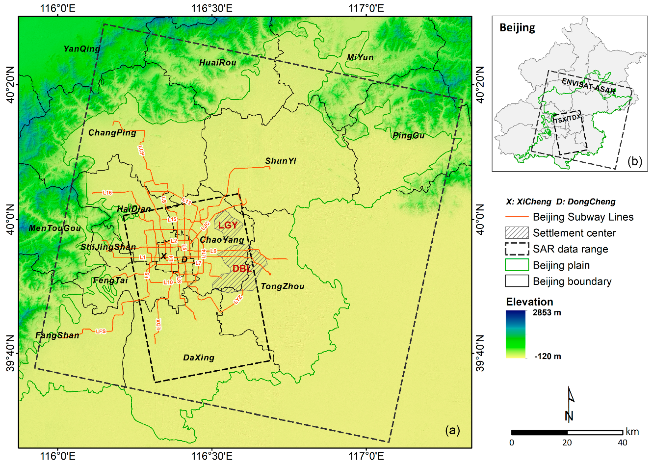
2.1. Study Area

Beijing is located in the north of the North China Plain (115.7—117.4° E, 39.4—41.6° N), and the terrain is high in the northwest and low in the southeast. The plain area covers an area of about 6300 square kilometers, with an average elevation of 43.5 m, and the resident population was 21.542 million in 2018 [22]. Beijing was the first city in China to build a subway, and the first line was officially opened in 1969 [23]. During the past 10 years, with the acceleration of urbanization, the infrastructure of Beijing has been continuously improved, especially regarding the planning and construction of rail transit, making it one of the most densely populated cities in China. By the end of 2017, Beijing had 19 subway lines in operation (Figure 1), with a total length of 574 km. It is reported that the rail transit distance in Beijing will reach 1000 km by 2030. In this study, the vector data of the BSN without deviation is downloaded from BIGMAP [24]. BIGMAP is a basic GIS industry application software that can download Google HD satellite maps, electronic maps, topographic maps with contour lines, road networks, water systems, building contours, and POI information among other vector data. At the same time, the downloaded satellite HD village map can see the house door, downloaded from any range.

Beijing is also a city with serious and uneven land subsidence. In the eastern part of the Beijing plain, the two most serious subsidence centers, Laiguangying (LGY) and Dongbalizhuang-Dajiaoting (DBL), have emerged, as shown in Figure 1 [25]. Many studies of the ground subsidence along the Beijing subway have been performed. However, all of these studies are based on single-sensor MTI techniques to obtain subway deformation information, and most of the monitoring time sequences are limited to fewer than 10 years.

2.2. Dataset

In 2003, the Beijing subway entered a period of large-scale construction. In the period since then, the variety of SAR satellites use has gradually increased, and the spatial resolution has continuously improved. To monitor surface deformation along the Beijing subway from 2003 to 2018, we selected two kinds of radar datasets that cover the major Beijing Subway Lines. The first is ENVISAT-ASAR (ASAR), from Jun 2003 to September 2010. ASAR, an Earth observation satellite of the European Space Agency (ESA), was launched in 2002 and lost contact in 2012. The other is TerraSAR-X/TanDEM-X (TSX/TDX), from April 2010 to October 2018. TSX is an X-band synthetic aperture radar satellite launched by Germany in 2007, and TDX is a sister satellite of TSX launched in 2010 with the same parameters as TSX. Both sister satellites are still currently in operation. The detailed parameter information of the two SAR datasets is shown in

Table 1. Acquisition parameters of the ENVISAT-ASAR and TSX/TDX data sets.

SAR Sensor	ENVISAT-ASAR	TSX/TDX
Orbit direction	Ascending	Descending
Operation mode	Image	Stripmap
Band (wavelength)	C(5.63)	X(3.11)
Resolution	30m	3m
Revisit cycle	35	11
Incidence angle 1	22.8°~22.9°	33.1°~33.2°
Polarization	VV	HH
Number of images	58	63
Temporal coverage	June 2003 to September 2010	April 2010 to October 2018

¹ In the calculation process, we rounded off the incidence angle (ASAS: 23°, TSX/TDX: 33°).

. Note that, prior to InSAR analysis, we clipped the SAR data, and the data coverage after clipping is shown in the black dotted line in Figure 1. We used the shuttle radar topography mission (SRTM) digital elevation model (DEM) with a spatial resolution of 90 m to remove the terrain phase and geocode the interferograms. Continuous leveling data from 2005 to 2013 (elevation measurement) and elevation change data using level monitoring from 2015 to 2016 and 2017 to 2018 were collected to verify the accuracy of InSAR analysis results. Compared with ASAR, TSX/TDX has high spatial resolution and can obtain a higher density of PS, especially for linear features such as subways, TSX/TDX can show more details of the subsidence center. Therefore, we selected PS obtained by TSX/TDX as the target set for extracting long-term sequence deformation information in the MMTI-TSF algorithm.

3. Methods

In this study, the improved MMTI-TSF algorithm was used to calculate the continuous deformation information of the study area from 2003 to 2018. The piecewise linear regression method was used to explore the deformation differential characteristics of the whole life cycle along the subway. The following is a detailed description of the two methods.

3.1. MMTI-TSF Algorithm and Improvement

There are at least three problems that need to be solved in MMTI-TSF [20]. First, due to the different incidence angles of different SAR sensors, the imaging geometries of different SAR sensors are also different. Second, the spatial location and coverage range of PS obtained by MTI processing is different for different SAR sensors. Third, the time reference selected by MTI analysis results from different SAR sensors is inconsistent. In addition, it is worth mentioning that the positions of the reference points used in the multi-sensor SAR data are usually difficult to keep consistent, while the selection of the reference point has a significant impact on the overall deformation monitoring results.

We introduced leveling data to address the problems with the reference points in the existing MMTI-TSF algorithm. The algorithm workflow is shown in Figure 2, including the MMTI-TSF before and after improvement.

The detailed description of the algorithm is as follows: (the time-series fusion of two kinds of SAR data is taken as an example to discuss the algorithm flow, three or more kinds of MMTI-TSF is an expansion of the approach used for two kinds)

i.

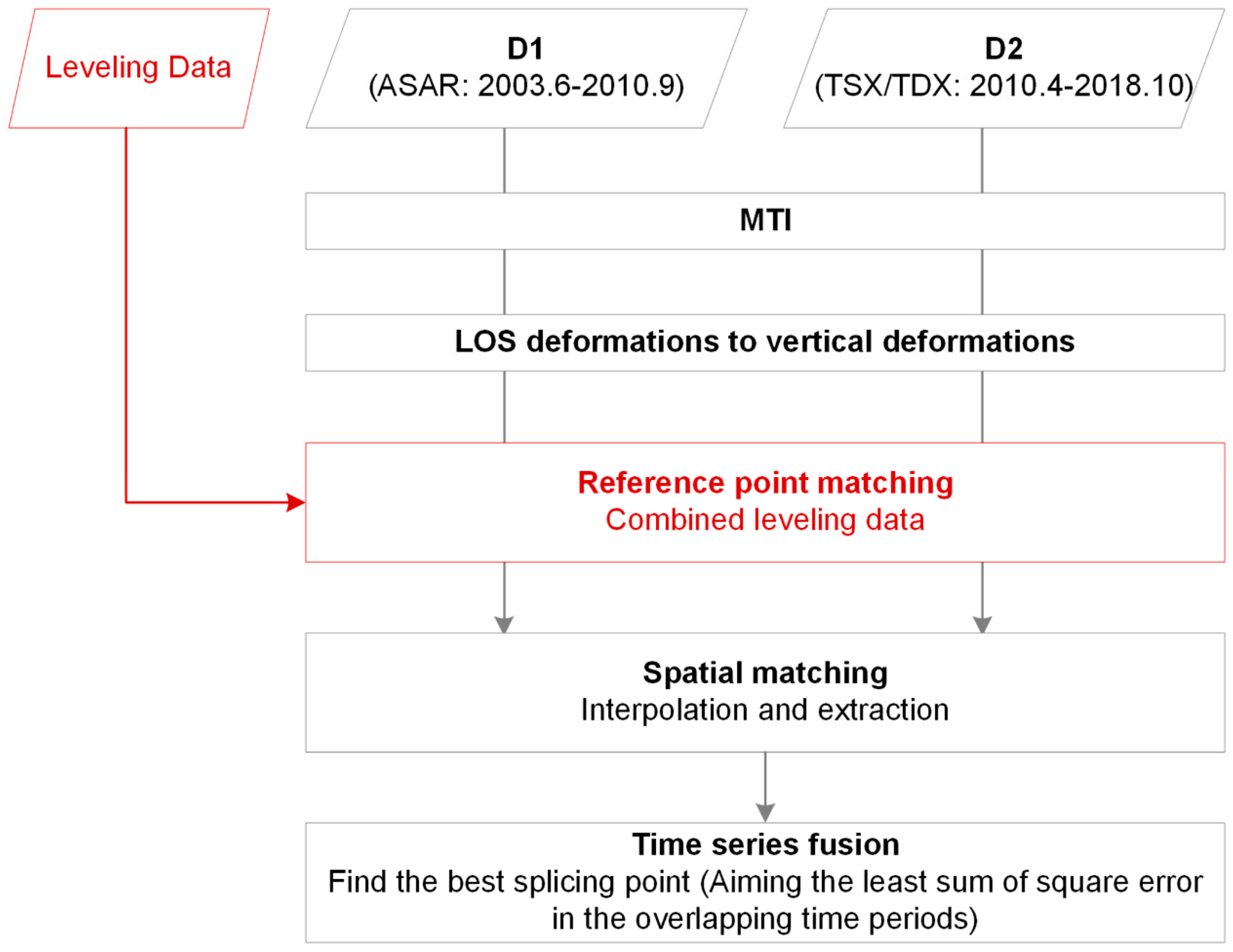
Multi-temporal InSAR (MTI) was used to obtain time-series deformation results of two kinds of SAR data, as shown in Figure 2 $D1$ and $D2$ are the two data sets are required to have overlapping periods.

MTI is a technique developed based on InSAR that uses multi-view SAR images to achieve high-precision, high-density measurement point extraction, and analysis. It is especially suitable for urban land subsidence and infrastructure deformation monitoring [16]. Many software programs have been developed to implement this algorithm, such as ISCE, StaMPS, ENVI, Doris, GAMMA, and SARProz.

In this study, interferometric point target analysis (IPTA) of Swiss synthetic aperture radar processing software GAMMA was used to process ASAR data [26]. The Quasi-Permanent Scatterers (QPS) of SARProz was used to process TSX/TDX data [27]. These two methods have been applied and confirmed by many InSAR researchers [18,28]. Since IPTA and QPS both use linear deformation models, and use amplitude dispersion to select points [16], they can be used in a multi-sensor time-series fusion algorithm, without considering the error caused by the different MTI algorithms.

ii.

InSAR is a side-view observation technique, and its direct observation result is line-of-sight (LOS) deformation, that is, the vector sum of the projections of the ground surface in the east, north, and vertical deformation variables in the radar line of sight. The LOS deformation observed by InSAR can be expressed as the following equation [29]:

$$d_{LOS}=d_U\cos \theta -d_N\sin \theta \cos \left(\alpha -\frac{3\pi }{2}\right)-d_E\sin \theta \sin \left(\alpha -\frac{3\pi }{2}\right),$$

(1)

where $d_{LOS}$, $d_U$, $d_E,$ and $d_N$ represent LOS, vertical, east, and north deformations, respectively. θ is the radar incident angle, and α is the angle between the satellite heading and north in a clockwise direction.

Different SAR sensors have different incidence angles. To eliminate this difference, we transformed LOS deformation into vertical deformation. There are many ways to address the issue of vertical deformation [30]. Simplified calculations can also be performed for different geological environments [21].

Xie J. et al.’s [31] GPS measurement results show that there is no obvious east–west or north–south deformation in Beijing. In this study, we converted LOS to vertical deformation by ignoring the horizontal deformation to eliminate the imaging geometric differences between $D1$ and $D2$ (which is necessary to ensure that the horizontal deformation in the study area is small enough to be ignored). The conversion formula is shown in Equation (2).

$$d_U=d_{LOS}/\cos \left(\theta \right),$$

(2)

iii.

Next is the improvement of the MMTI-TSF algorithm (marked in red in Figure 2). The key to MTI deformation analysis is the selection of the reference point. The different resolutions of different SAR platforms and the difference in MTI analysis processes will inevitably lead to a certain deviation of the reference point position. This difference will have a large impact on the fusion result. However, the elimination of this difference is rarely noticed in the previous multi-sensor MTI time-series fusion algorithms.

It is well know that external leveling data is a relatively accurate means of deformation measurement. Therefore, using external leveling data to unify the reference point is a more reliable method when data is available. If there is a lack of leveling data using one of the reference points as a reference to calibrate another MTI analysis result can also be considered.

In this study, the uniform reference point position was determined by referring to the external leveling data, and then the vertical deformation of the two sets of time series data were recalculated based on this reference point.

iv.

Spatial interpolation and raster extraction to vector points were used to register two sets of PS with spatial distribution differences. To improve the spatial resolution after matching, we took the PS obtained from the SAR data of lower resolution ($D1$) as the spatial interpolation object, and then took the PS obtained from the SAR data of higher resolution ($D2$) as the target set of vector extraction. The interpolation algorithm adopts the inverse distance weighted (IDW) interpolation. In this study, the time series results of ASAR were interpolated into the PS set obtained by TSX/TDX.

v.

Finally, according to the principle of minimum error sum of squares of overlapping periods, the optimal splicing time was selected to convert the values of two relative time series into absolute time series. The optimization criterion is shown in Equation (3).

$$\min \left[{\sum }_{i=1}^m{(d_i^1-d_i^2)}^2\right],$$

(3)

where $m$ represents the number of time nodes common to the two sets of time series in the overlapping period, and $d_i^1$ and $d_i^2$, respectively, represent the cumulative deformation variables corresponding to two different data sets at the time $i$. It is worth noting that we used the same month and the minimum number of days as the standard to perform a one-to-one correspondence between the two sets of data in the overlapping period, and the maximum did not exceed 30 days (In this study, the overlapping period of $D1$ and $D2$ is from April to September 2010. We consider that August 5 of $D1$ and August 20 of $D2$ are the corresponding moments instead of July 31). If a certain group of data in the overlapping period is missing a certain month, the deformation result of the lack of the corresponding month is calculated by the average method (For example,$D1$ has data for $d_4^1$, $d_5^1$, and $d_6^1$ and $D2$ only has $d_4^2$ and $d_6^2$ months. To find $d_5^2$ corresponding to $D1$, we consider $\left[d_4^2+\left(d_6^2-d_4^2\right)/2\right]$ as $d_5^2$). Through iterative calculation, it is concluded that $t_0$ at the minimum of the above formula is the optimal splicing point, and then the deformation difference at the splicing point is calculated, $\Delta d=d_{t_0}^1-d_{t_0}^2.$ The time sequence result ($D1$) to be interpolated starts at time $t_0$. If $D1$ is in the first half of the whole period, it shifts up the unit length of $\Delta d$, and vice versa. Finally, the result was converted to a long time series continuous deformation with the starting time as the shape variable of 0.

3.2. Piecewise Linear Regression

The core of piecewise linear regression analysis is to use a piecewise linear function to describe the trend of a series of scattered points [32]. Assuming that the deformation along the subway shows different trends during different life stages of the subway, then piecewise linear regression is an effective means to identify this difference. Under this assumption, we use piecewise linear regression to identify the deformation characteristics of different life stages of the Beijing Subway Line 6 Phase I project (L6-I).

For the relationship between the response variable ($Y$) and the explanatory variable (X), different linear relationships may apply to different $X$ ranges. A single linear model cannot adequately describe this relationship. Nonlinear models are usually the most appropriate in this case, but sometimes there is an obvious breakpoint between two different linear relationships. Piecewise linear regression is a form of regression that allows multiple linear models to fit data in different $X$ ranges. Assuming a segment occurs at $t^{\ast }$, dummy variables are used to estimate the slope of each segment. We set the following form of dummy variables:

$$D_t=\{\begin{array}{c}0, (t<t^{\ast })\\ 1,\left(t\ge t^{\ast }\right)\end{array},$$

(4)

The piecewise linear regression model to be estimated is written as:

$$Y_t={\beta }_0+{\beta }_1{X}_t+{\beta }_2\left(X_t-X_{t^{\ast }}\right)D_t,$$

(5)

where ${\beta }_0$ is the intercept, and ${\beta }_1$ and ${\beta }_2$ are the slopes of the two piecewise fitted straight lines.

In this study, we first draw a scatter plot of the deformation time series of a typical subway station. According to the distribution of the scatterplot, we have identified two sites with segmented features and determined $t^{\ast }$. Then, we use the piecewise linear regression to calculate the difference in deformation rate in each period.

4. Experimental Results and Analysis

Using the improved MMTI-TSF algorithm, we completed the time series deformation mapping of Beijing from 2003 to 2018, and analyzed the monitoring results (Section 4.1). Based on these results, we realized the health diagnosis of the Beijing subway network during the past 15 years (Section 4.2). We focused on the life-cycle deformation characteristics of Beijing Subway Line 6 with severe uneven subsidence (Section 4.3).

4.1. Mapping and Analysis of InSAR Results

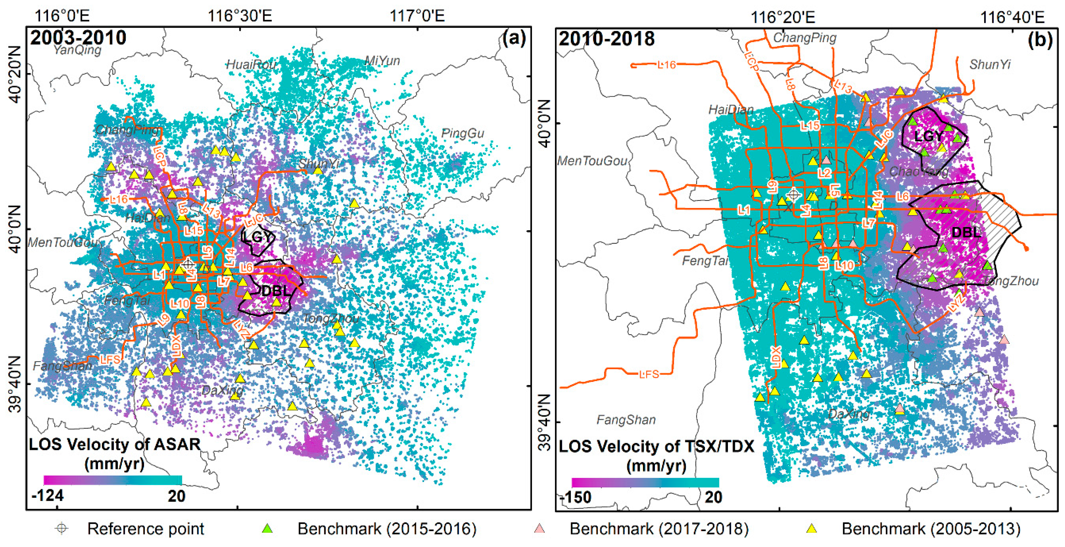
4.1.1. MTI Results

We plot the linear deformation rates of MTI_ASAR and MTI_{TSX/ TDX} in Figure 3a,b, respectively. In Figure 4, the black ellipses circle the two major subsidence centers in Beijing, Laiguangying (LGY), and Dongbalizhuang-Dajiaoting (DBL). From Figure 3, we can visually compare the subsidence status of the two subsidence centers at different periods. The results show that the PS density obtained by ASAR is about 28 per square kilometer. From June 2003 to September 2010, the maximum cumulative subsidence amount and the maximum sedimentation rate, respectively, of 900 mm and 124 mm/year occurred in DBL. Due to the small spatial resolution of ASAR, many monitoring holes in the subsidence center cannot capture its deformation information. The PS density obtained by TSX/TDX is 516 per square kilometer. It was found that the subsidence in LGY and DBL was still relatively large from April 2010 to October 2018. The maximum cumulative subsidence and maximum subsidence rate were 1250mm and 150 mm/year, respectively, and also occurred in DBL. It can be seen that the spatial distribution characteristics of the subsidence rates in Beijing from 2003 to 2010 and 2010 to 2018 are consistent, and appear uneven. The main subsidence areas are located in the two regions of LGY and DBL, which agrees with previous research results [25,33].

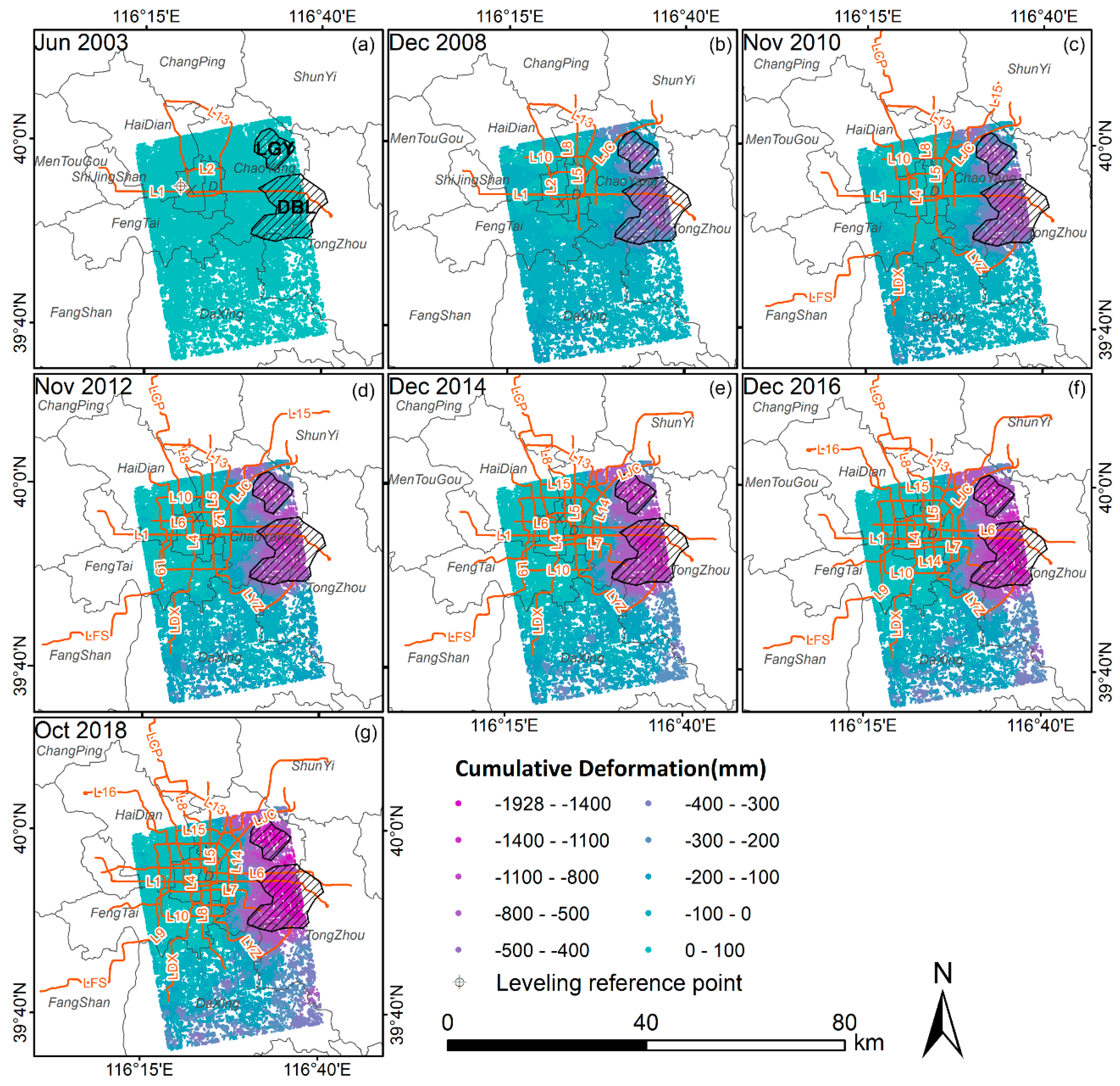
4.1.2. MMTI-TSF Results

The time series of InSAR deformation monitoring after MMTI-TSF fusion was used for a 15 year period. During this period, Beijing’s land subsidence increased and the number of subway lines increased from 3 to 18. We superimposed the time series evolution of the BSN and the space-time evolution of subsidence as shown in Figure 4a–g. After fusion, the number and spatial distribution of PS are consistent with those obtained by high-resolution satellite TSX/TDX (Figure 3b). The results show that from June 2003 to September 2018 there was a significant uneven subsidence in the study area, with a maximum cumulative subsidence of 1.9 m and the formation of two main subsidence centers (Figure 4 LGY and DBL), which is consistent with the results of the MTI analysis (Figure 3). In addition, combined with Figure 4a, it was found that there are six subway lines (L1, L6, L7, LJC, L15, LYZ) in Beijing all passing through the area with severe subsidence. In particular, the eastern section of L1 and L6 is almost completely within the DBL subsidence center, the largest subsidence center in Beijing, while the subsidence along the western and middle sections is not obvious. L1 was the first subway line to be opened to traffic (1969) in Beijing. It crosses the subsidence center and is still in stable operation. InSAR results show that the section of L1 with a cumulative subsidence greater than 500 mm is about 9.6 km long, mainly located between Sihui East Station and Baliqiao Station. L6 also passes through the subsidence center, but was only opened to traffic on the main road in 2014. InSAR results show that the section with a cumulative subsidence greater than 500 mm along the L6 line is about 8 km long, mainly between Qingnian Road Station and Caofang Station. Based only on the subsidence rate, L1 and L6 have the same safety risk. Regional uniform subsidence or non-subsidence has little effect on the subway, while regional uneven subsidence is the most worthy of consideration in future subway construction and safe operation. For this reason, Section 4.2 quantitatively analyzes the status of uneven subsidence along the Beijing Subway.

4.2. Beijing Subway Network

The deformation of the lower soil mass will undoubtedly affect the stability of the upper subway track. The burial depth of the Beijing subway is predominantly between 40 and 60 m, and the main contribution of the ground subsidence is about 100 m to 180 m [34]. Therefore, identifying the ground subsidence characteristics along the Beijing subway is necessary for the safety of the subway and its surrounding infrastructure. It is well known that, the linear subsidence rate effectively reflects the trend and degree of deformation in the study area. Zhu X. et al. [35] used TerraSAR-X to study the deformation status of the BSN from April 2010 to December 2016, and found that the maximum subsidence rate of the Beijing subway line exceeded 100 m/year. Furthermore, the gradient of the subsidence rate can quantitatively reveal the spatial non-uniformity of the deformation zone. In this study, we selected two indicators to identify subway stability: linear deformation rate (Figure 5a) and deformation rate gradient (Figure 5b). We used Slope, an ArcGIS spatial analyst tool, to calculate the gradient.

According to the statistics in Figure 5a, the number of PS along the BSN within the coverage area of TSX/TDX is ±5 mm/year, accounting for about 70% of the total number of PS along the subway in the study area. It shows that the underground environment along the Beijing Subway is stable, and the subway only shows a large trend of subsidence along the section of the subsidence center. The subsidence along L1 is the most serious, with a maximum subsidence rate of 115 mm/year, followed by L6, with a maximum subsidence rate of 80 mm/year. Figure 5b shows the gradient change graph calculated based on the linear deformation rate. The results show that, although the subsidence rate along the eastern section of L1, L7, LYZ, LJC, and L15 is high, the deformation gradient changes are small, all below 0.002 degrees, indicating that the uneven deformation along these lines is weak and the stability is good. However, the gradient of the L6 deformation rate varies greatly in different sections, up to 0.005 degrees, and is mainly concentrated in the eastern section of L6-I (Figure 6). In the next section, we focus on the spatiotemporal evolution characteristics of ground subsidence along L6.

4.3. Beijing Subway Line 6

Beijing Subway Line 6 (L6) has a total length of 52.9 km, 34 stations, and is spread east–west. The construction of L6 was completed in three phases. The first phase (L6-I, as shown by the red line in Figure 6a) starts at Haidian Wuluju Station and ends at Caofang Station. Construction started at the end of December 2007 and the section officially opened for operation at the end of December 2012. The second phase of the project (L6-II, as shown in Figure 6a green line section) starts at Caofang Station and ends at Lucheng Station. Construction started in February 2011 and officially opened in December 2014. The third phase of the project (L6-III, the blue line in Figure 7a) starts at Haidian Wuluju Station and ends to the west at Jin’anqiao Station. Construction started in December 2013 and the line officially opened for operation in December 2018. Since L6 traverses DBL, the largest subsidence center in Beijing (Figure 5 DBL), many researchers have investigated the subsidence characteristics along the line. For example Chen, Z. et al. [6] used TerraSAR-X data to study the deformation characteristics of the Line 6 Phase II project from 2011 to 2015, and concluded that the excavation of subway stations has a great impact on the surrounding environment. Liu K. et al. [36,37] used the InSAR monitoring results from 2013 to 2015 to evaluate the danger of L6, and found that the L6 operation safety level was high during this period. However, there are few studies of deformation monitoring for the entire L6 life cycle.

In this study, the obtained InSAR deformation information mainly covers L6-I, and the monitoring time spans the full life cycle of L6-I, from 2003 to 2018, as shown in Figure 6b. We define the “full life cycle” of L6-I as encompassing the preparation period (6/2003–12/2007), construction period (12/2007–12/2012), and operation period (12/2012–10/2018). We use 20 m as the sampling interval to extract the deformation rate gradient values at equal intervals on the subway line and draw the deformation rate gradient profile of Line 6 as shown in the broken line of Figure 6b. The results show that the deformation gradient of the east section of L6-I changes greatly, especially from Jintailu Station (see Figure 6(bC)) to Caofang Station (see Figure 6(bG)), where the deformation gradient fluctuates from 0.001 degrees to 0.0055 degrees. This proves that, from 2003 to 2018, the uneven deformation of the L6-I east section is large.

The four main stations located in the deformation rate gradient of the eastern section of L6 (Jintailu C, Shilipu D, Changying F, and Caofang G in Figure 6) were selected to analyze the time-series deformation evolution characteristics of the subway during different life stages. Using the method of piecewise linear regression, the time series deformation results of the station were analyzed in pieces, as shown in Figure 7.

Figure 8a shows a piecewise linear fitting result of Shilipu Station (D) and Jintailu Station (C) with a small deformation rate gradient at the edge of the center of the DBL subsidence. The black triangles shows the timing monitoring results of the leveling points (Figure 7(aS1)) near Jintailu Station, and the black line is the fitting curve. The deformation timing of the two sensors is consistent with the leveling result in the trend, but the leveling point S1, which is about 1km from the subway, does not have obvious segmentation characteristics. Comparing C and D, we found that although the two have different subsidence rates, they both changed suddenly at the same time in August 2010 during the L6-I construction period (Figure 8a, II). Considering that the MMTI-TSF algorithm may affect the subsidence timing result, we selected the Changying station (F) and Caofang station (G) close to the DBL subsidence center in the same way to perform piecewise linear fitting and drew the measurement results of the nearby leveling point (as shown in Figure 7(aS2)). The results showed that there was no segmentation feature in Figure 8b. This eliminates the calculation error in the subsidence timing caused by MMTI-TSF. Therefore, we infer that the subsidence trend of the subway station may be related to its position from the subsidence center. Along the subway line close to the subsidence center, irrespective of the life period of the subway, the subsidence of the area itself plays a leading role. The subsidence along the subway at the edge of the subsidence center exhibits different characteristics in different life periods. For instance, the subsidence along the subway during construction will be further aggravated before gradually stabilizing during the operation period.

5. Validation and Discussion

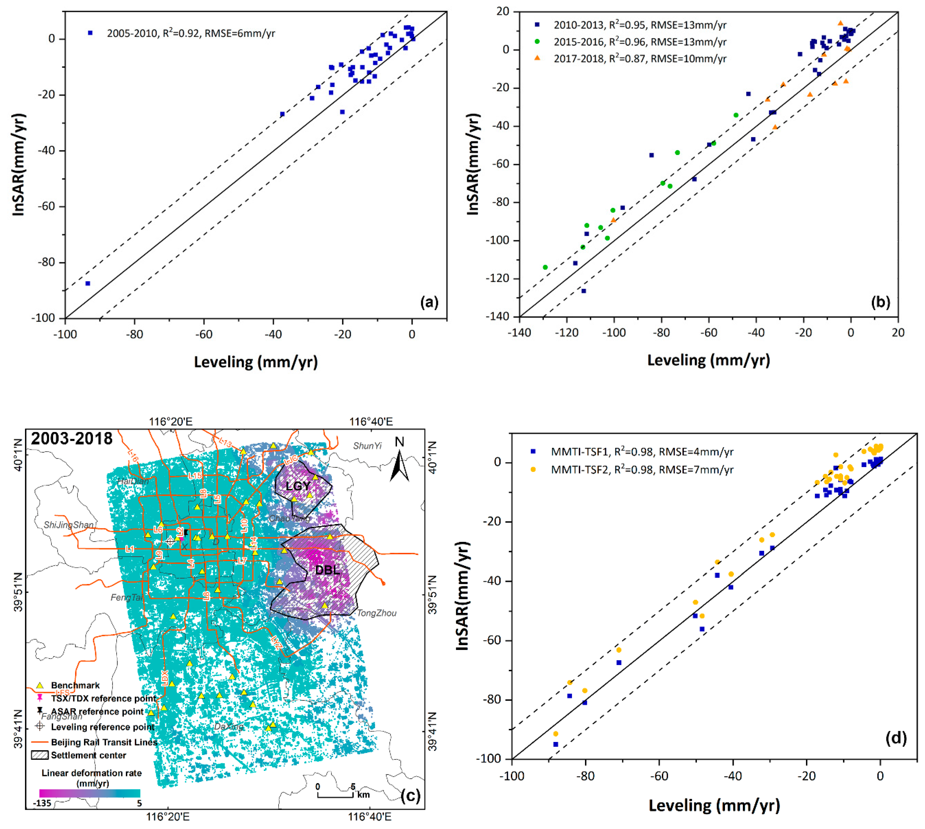
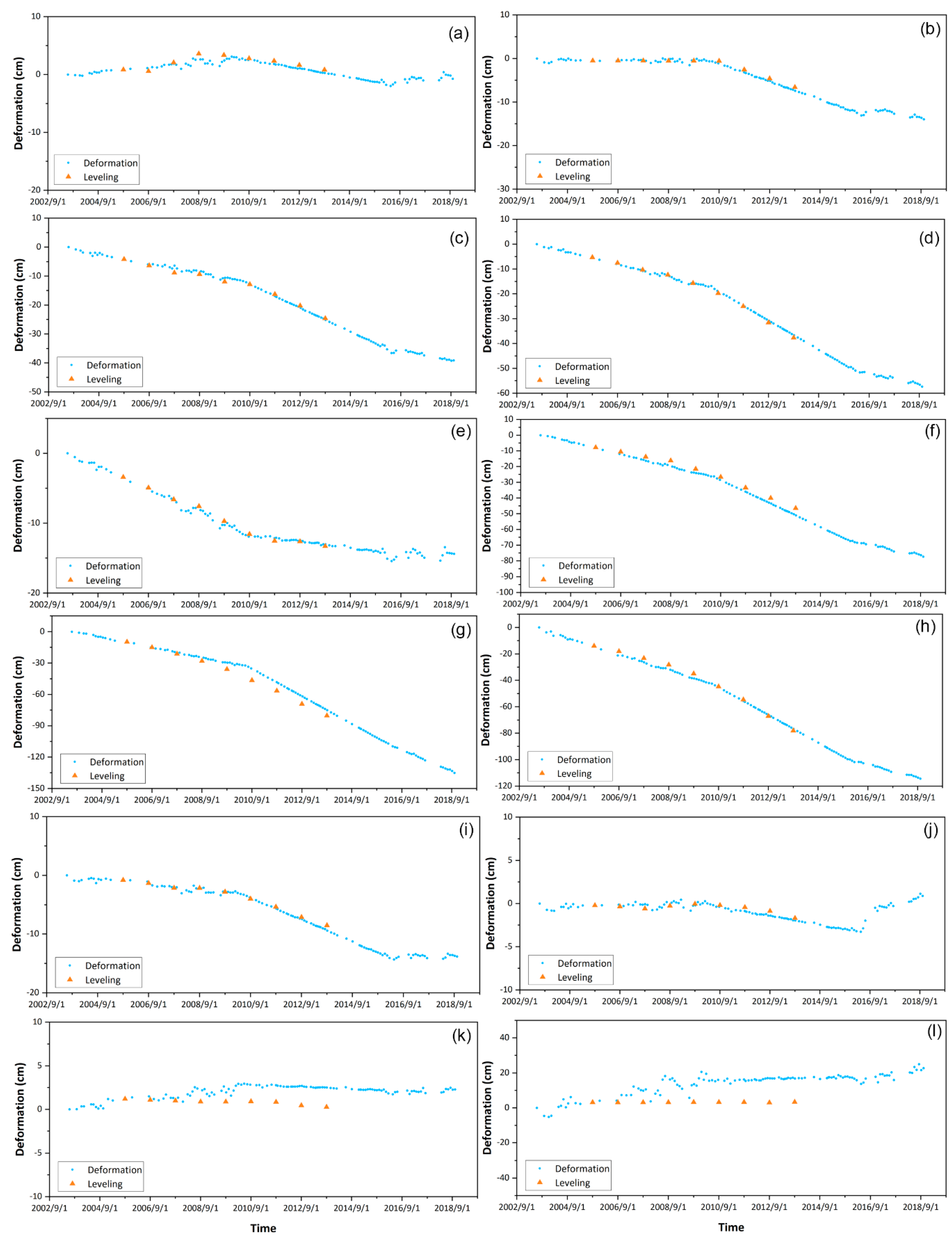
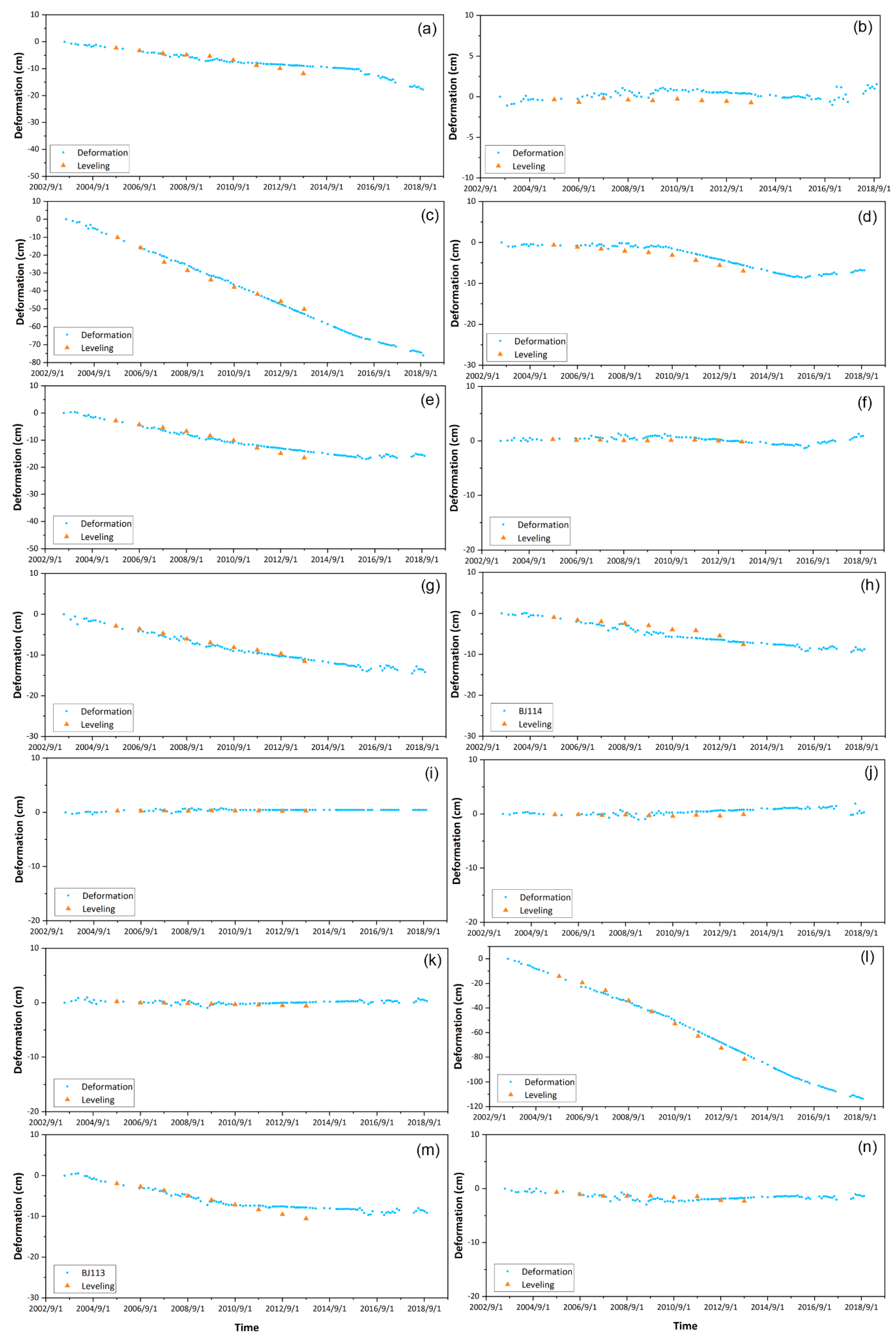
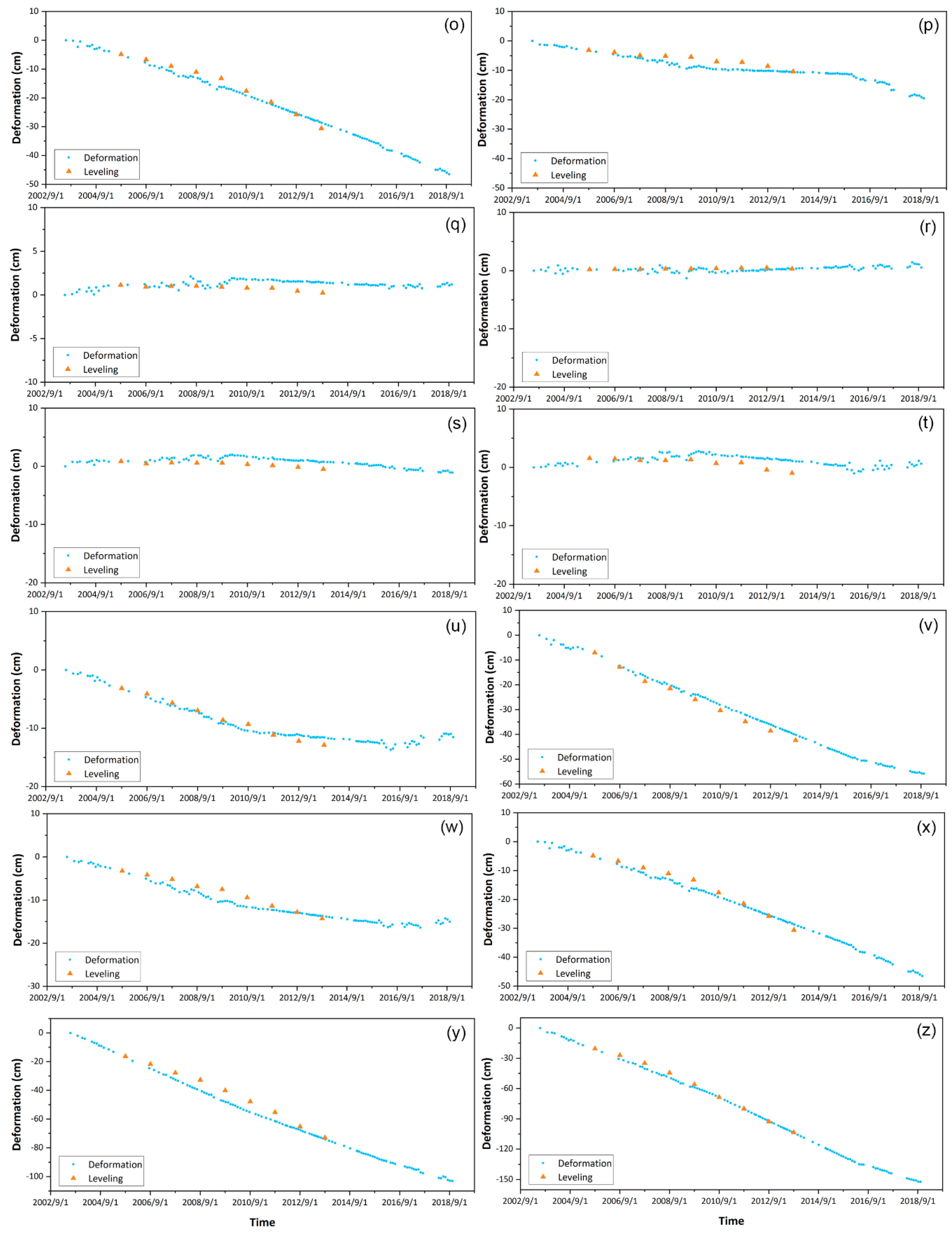
5.1. Validation

Leveling is a ground deformation measurement method independent of InSAR analysis and can be used to evaluate the accuracy of InSAR analysis. First, we evaluated the consistency of the linear deformation rate between the level monitoring data and the InSAR analysis results by calculating $R^2$ and root mean square error ($\mathrm{RMSE}$). The deformation results obtained by MTI will directly affect the accuracy of the fusion results. We evaluated the time-series InSAR analysis results obtained by the two previous SAR sensors, as shown in Figure 8a (ASAR), Figure 8b (TSX/TDX). It is concluded that the accuracy of InSAR deformation information acquired by ASAR is higher, RMSE = 6 mm/year, while the accuracy of the results obtained by TSX/TDX is lower. Subsequently, the long-time InSAR analysis results after MMTI-TFS fusion were evaluated. We used the least-squares linear fitting method to calculate the linear deformation rate over a period of 15 years, as shown in Figure 8c. Similarly, we evaluated the accuracy of the fusion result (as shown in Figure 8d-MMTI-TSF1), RMSE = 4 mm/year. In addition, we also calculated the accuracy of the unimproved MMTI-TSF (black text in Figure 2) for cross-validation (Figure 8d-MMTI-TSF2) and obtained RMSE = 7 mm/year. It is concluded that MMTI-TSF improved the InSAR monitoring accuracy to a certain extent while prolonging the InSAR monitoring timing, and that it can provide a reliable technical means for monitoring city security, especially regarding infrastructure.

To further investigate the accuracy of the InSAR monitoring results after fusion, we superimposed the timing deformation of each level point and its nearest PS. According to the characteristics of different precision comparison results, we divided the 38 verification result graphs into two parts. The verification results in Part 1 (Figure 9) show that the fused InSAR monitoring results and the leveling monitoring results are all show obvious segmentation characteristics, especially from Figure 9a–j). However, there are also some with poor accuracy comparison, as shown in Figure 9k and Figure 1. Under the premise that the overall accuracy is credible, we think this may be caused by an error in the leveling. In part 2 (Figure 10), the deformation results monitored by InSAR after fusion are well fitted in term of the timing of leveling points, especially the transition period of the stitching of the two data sets (around 2010), which further proves the accuracy of MMTI-TSF in regard to timing. Furthermore, we found that, compared with the horizontal monitoring data, the fused InSAR results could detect information with greater detail. Especially in identifying deformation mutation points, the fusion InSAR results are more advantageous. Therefore, MMTI-TSF can provide reliable technical support for monitoring the continuous deformation of linear features, which is worthy of popularization and application.

5.2. Limitations and Uncertainties of MMTI-TSF

The MMTI-TSF algorithm is very flexible and can handle SAR satellite data from multiple sensors. It has the advantages of high resolution and high accuracy in monitoring long-term ground displacements. Meanwhile, the algorithm is also subject to limitations and uncertainties.

In the process of MTI analysis of multi-sensor SAR satellite data, it is necessary to select a suitable MTI algorithm. In order to ensure the consistency of the multi-sensor MTI analysis results, it is desirable to choose the same MTI algorithm for processing. In this study, two similar MTI algorithms were used to process two SAR datasets separately, which inevitably creates errors regarding the results. Results verification shows that the accuracy of InSAR deformation information on ASAR and TSX/TDX are different, which indicates that different MTI algorithms will bring certain uncertainties of the results. During the transformation from LOS deformation to vertical deformation, it is worth noting that a basic survey of the surface deformation characteristics of the study area is required. This experiment simplified the calculation of vertical deformation under the premise that the horizontal deformation in the study area were negligible. If the horizontal deformation cannot be ignored, the solution process will be more complicated. This is where the MMTI-TSF algorithm is worth improving on in the future. In the process of reference point matching, the external leveling point must be stable or a recognized non-sedimentation point, otherwise, new errors will be introduced into the fusion result. In the absence of external leveling points, the reference point selected by one of the sensors in the MTI algorithm can be used as a reference to convert the reference point of the MTI analysis results of other sensors. In the process of spatial matching, we used spatial interpolation and extraction to match the PS spatial position of multiple sensors. In practice, there are certain uncertainties of this method, including the selection of interpolation algorithms and the selection of parameters. Furthermore, the spatial resolution of the sensor is also important for the spatial location matching. Some experts have proposed using the same name point matching algorithm to solve the problem of spatial location matching [29]. No matter which method is chosen, spatial matching will definitely bring errors, which is inevitable. In the process of time series fusion, in order to ensure that the single-sensor MTI analysis of settlement change characteristics does not change, we used the method of finding the best stitching point. There are many alternative methods, such as machine learning, nonlinear fitting, etc. In addition, the MMTI-TSF model used in the study is based on the interferometry results of two SAR satellites with overlapping periods. For time-series stitching without overlapping periods, bidirectional prediction is a desirable solution. It should be clear that different fusion methods have different characteristics and advantages and are suitable for different research objects. In summary, the MMTI-TSF algorithm is immature, and would benefit from further in-depth examination and research.

6. Conclusions

This paper systematically expounds on the MMTI-TSF algorithm. By introducing leveling data, the accuracy of the existing MMTI-TSF techniques is improved and the spatiotemporal resolution of MTI analysis results is improved. Using the improved MMTI-TSF analysis results, the spatiotemporal evolution characteristics of Beijing subway network and its uneven subsidence along the line were analyzed for the first time in 15 years. We obtained the following conclusions:

• The MMTI-TSF algorithm can fuse multi-sensor MTI monitoring results, and improve spatial resolution with low cost, which is conducive to the monitoring of the entire life cycle deformation of urban infrastructure, especially linear features. Furthermore, the improved MMTI-TSF algorithm can obtain higher deformation monitoring accuracy ($R^2=98\%,$ RMSE = 4 mm). Nonetheless, the MMTI-TSF algorithm also has some limitations and uncertainties. It is still immature and requires flexible application in terms of wide applicability.
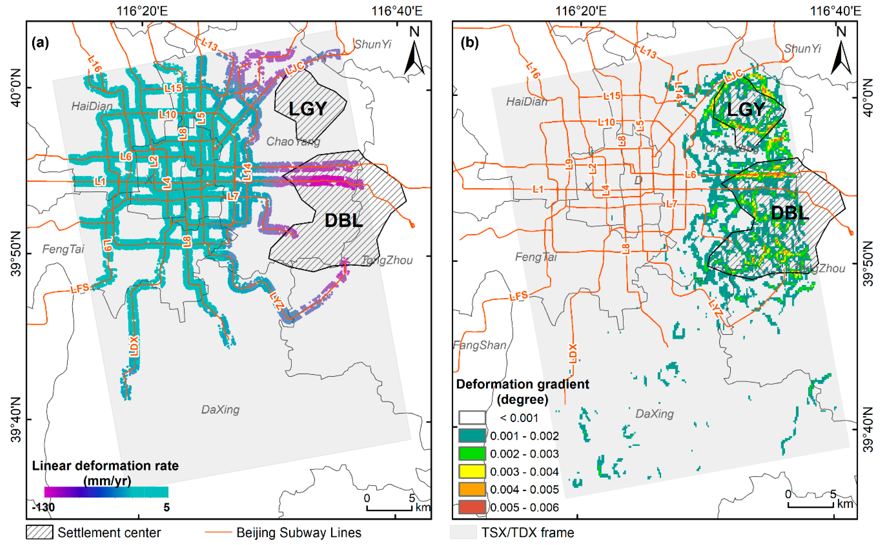
• In the area along the Beijing Subway, the subsidence in the east is more severe than that of the west, and the uneven deformation is obvious. The urban rail transit planning and safety departments should pay special attention to deformation monitoring of subway lines that are distributed east–west, such as Line 1 (L1), Line 6 (L6), Line 7 (L7), and the airport line (LJC), prior to further railway planning and construction. L6, in particular, shows evidence of serious uneven deformation.
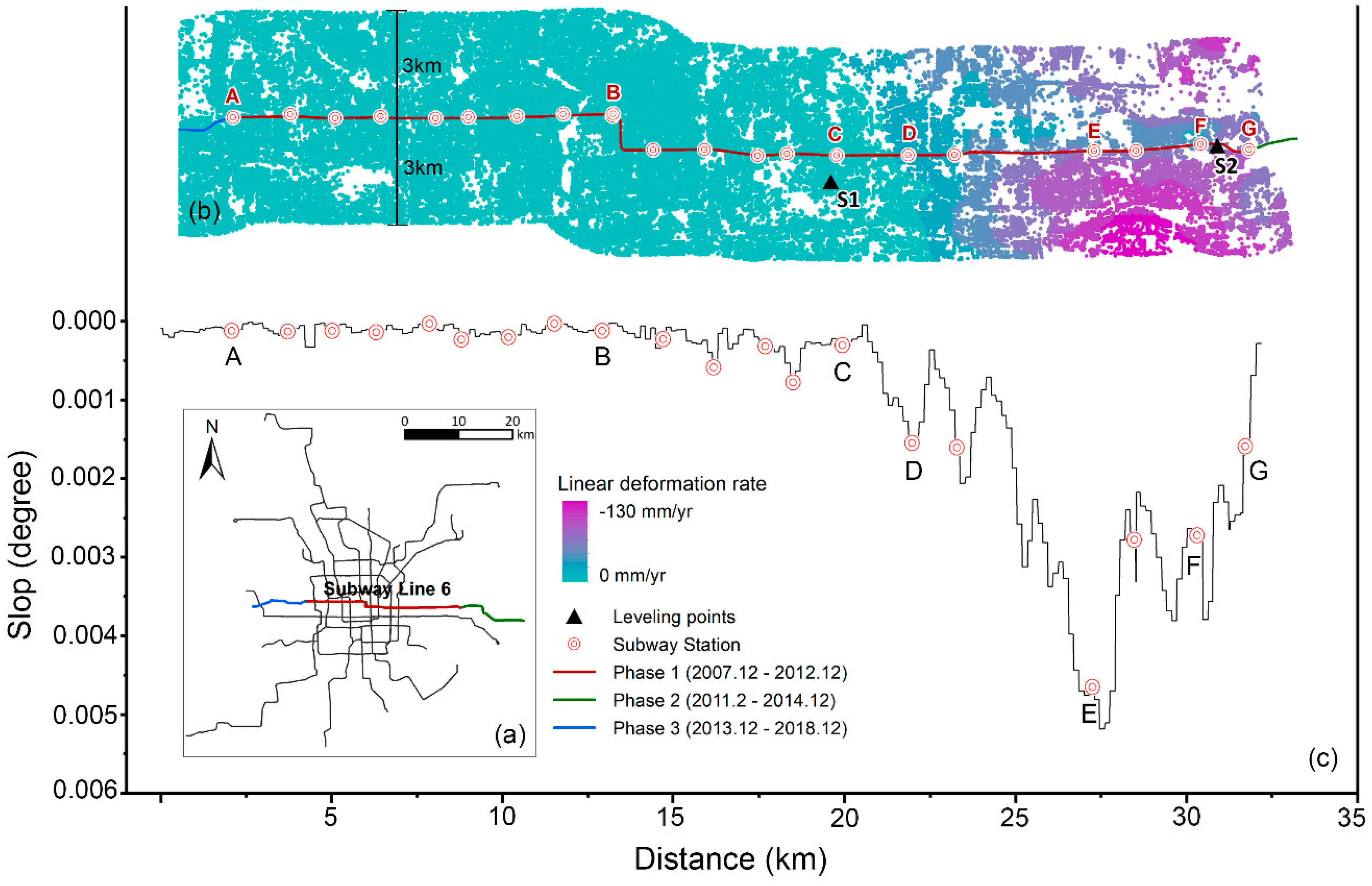
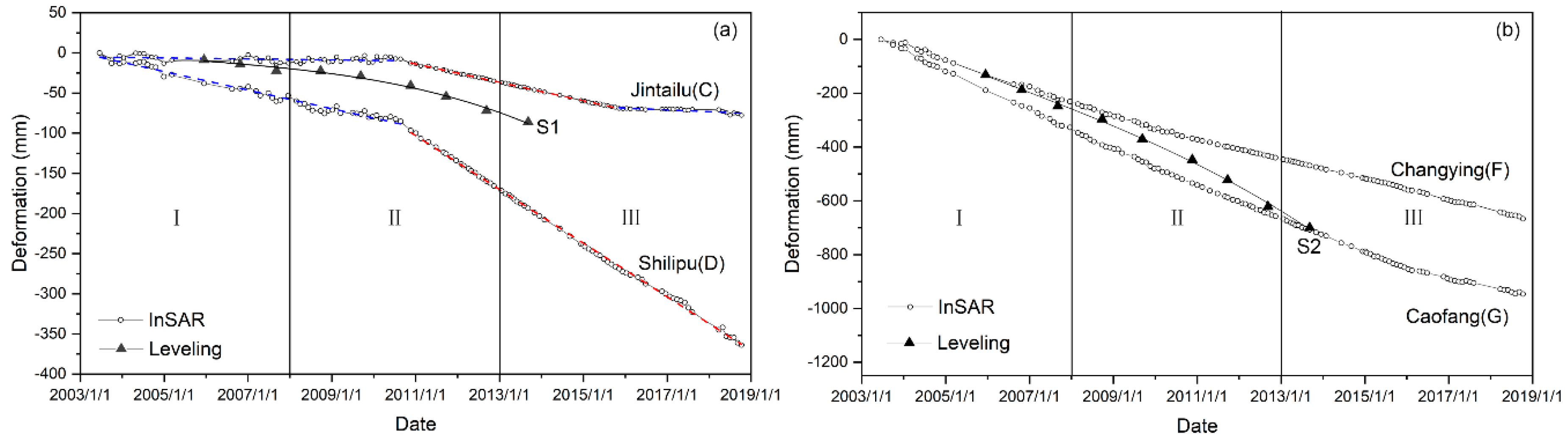
• The deformation characteristics of the first phase of L6 (L6-I) during the entire life cycle of the subway are related to its position from the subsidence center. The segmentation characteristics are seen at the edge of the subsidence center: the deformation rate during the early stage of construction was less than 10 mm/year, and increased significantly during the construction period and the initial stage of operation by about 69 mm/year, before gradually stabilizing. The deformation characteristics near the subsidence center are controlled by the subsidence center and have no segmentation characteristics. Therefore, for planning and construction of subways, the underground subsidence characteristics should be considered. Those near the subsidence center need to be well controlled throughout the process, while those located at the edge of the subsidence require special attention during the construction period to avoid accidents.

References

1. Osmanoğlu, B.; Dixon, T.H.; Wdowinski, S.; Cabral-Cano, E.; Jiang, Y. Mexico City subsidence observed with persistent scatterer InSAR. Int. J. Appl. Earth Obs. Geoinf. 2011, 13, 1–12. [Google Scholar] [CrossRef]
2. Amelung, F.; Galloway, D.L.; Bell, J.W.; Zebker, H.A.; Laczniak, R.J. Sensing the ups and downs of Las Vegas: InSAR reveals structural control of land subsidence and aquifer-system deformation. Geology 1999, 27, 483–486. [Google Scholar] [CrossRef]
3. Chen, M.; Tomás, R.; Li, Z.; Motagh, M.; Li, T.; Hu, L.; Gong, H.; Li, X.; Yu, J.; Gong, X. Imaging Land Subsidence Induced by Groundwater Extraction in Beijing (China) Using Satellite Radar Interferometry. Remote Sens. 2016, 8, 468. [Google Scholar] [CrossRef] [Green Version]
4. Dong, S.; Samsonov, S.; Yin, H.; Ye, S.; Cao, Y. Time-series analysis of subsidence associated with rapid urbanization in Shanghai, China measured with SBAS InSAR method. Environ. Earth Sci. 2014, 72, 677–691. [Google Scholar] [CrossRef]
5. Frangopol, D.M.; Saydam, D.; Kim, S. Maintenance, management, life-cycle design and performance of structures and infrastructures: A brief review. Struct. Infrastruct. Eng. 2012, 8, 1–25. [Google Scholar] [CrossRef]
6. Chen, Z.; Guangyao, D.; Zhenghui, Y.; Xuan, C.; Zhen, W. Deformation Monitoring and Law of Beijing Metro Line 6 (Phase II). In Proceedings of the 2018 Fifth International Workshop on Earth Observation and Remote Sensing Applications (EORSA), Xi’an, China, 17–20 June 2018; IEEE: Xi’an, China, 2018; pp. 1–5. [Google Scholar]
7. Pratesi, F.; Tapete, D.; Del Ventisette, C.; Moretti, S. Mapping interactions between geology, subsurface resource exploitation and urban development in transforming cities using InSAR Persistent Scatterers: Two decades of change in Florence, Italy. Appl. Geogr. 2016, 77, 20–37. [Google Scholar] [CrossRef] [Green Version]
8. Jia, X.; Gong, H.; Chen, B. Analysis of the Influence of Uneven Ground Subsidence on the Operation of Beijing Subway Line 15. Remote Sens. Inf. 2014, 29, 58–63. [Google Scholar]
9. Lee, E.S.; Lee, W.S.; Lim, K.M.; Bang, M.S. The Measurement of Railway Using VRS GPS. AMM 2013, 446–447, 1118–1122. [Google Scholar] [CrossRef]
10. Hwang, C.; Hung, W.-C.; Liu, C.-H. Results of geodetic and geotechnical monitoring of subsidence for Taiwan High Speed Rail operation. Nat. Hazards 2008, 47, 1–16. [Google Scholar] [CrossRef]
11. Abidin, H.Z.; Djaja, R.; Darmawan, D.; Hadi, S.; Akbar, A.; Rajiyowiryono, H.; Sudibyo, Y.; Meilano, I.; Kasuma, M.A.; Kahar, J.; et al. Land Subsidence of Jakarta (Indonesia) and its Geodetic Monitoring System. Nat. Hazards 2001, 23, 365–387. [Google Scholar] [CrossRef]
12. Alkaff, A.; Moreno, F.M.; José, L.J.S.; García, F.; Martín, D.; Escalera, A.D.L.; Nieva, A.; Garcéa, J.L.M. VBII-UAV: Vision-Based Infrastructure Inspection-UAV. In Recent Advances in Information Systems and Technologies; Springer: Berlin/Heidelberg, Germany, 2017. [Google Scholar] [CrossRef]
13. Hooper, A.; Zebker, H.; Segall, P.; Kampes, B. A new method for measuring deformation on volcanoes and other natural terrains using InSAR persistent scatterers. Geophys. Res. Lett. 2004, 31. [Google Scholar] [CrossRef]
14. Bürgmann, R.; Rosen, P.A.; Fielding, E.J. Synthetic Aperture Radar Interferometry to Measure Earth’s Surface Topography and Its Deformation. Ann. Rev. Earth Planet. Sci. 2000, 28, 169–209. [Google Scholar] [CrossRef]
15. Hooper, A. A multi-temporal InSAR method incorporating both persistent scatterer and small baseline approaches. Geophys. Res. Lett. 2008, 35, L16302. [Google Scholar] [CrossRef] [Green Version]
16. Lin, H.; Ma, P.; Wang, W. Introduction of Spaceborne MT-InSAR Method for Monitoring the Health of Urban Infrastructure. Acta Geod. Cartogr. Sin. 2017, 46, 1421–1433. [Google Scholar]
17. Qin, X.; Yang, M.; Zhang, L.; Yang, T.; Liao, M. Health Diagnosis of Major Transportation Infrastructures in Shanghai Metropolis Using High-Resolution Persistent Scatterer Interferometry. Sensors 2017, 17, 2770. [Google Scholar] [CrossRef] [PubMed] [Green Version]
18. Perissin, D.; Wang, Z.; Lin, H. Shanghai subway tunnels and highways monitoring through Cosmo-SkyMed Persistent Scatterers. ISPRS J. Photogramm. Remote Sens. 2012, 73, 58–67. [Google Scholar] [CrossRef]
19. Wang, H.; Feng, G.; Xu, B.; Yu, Y.; Li, Z.; Du, Y.; Zhu, J. Deriving Spatio-Temporal Development of Ground Subsidence Due to Subway Construction and Operation in Delta Regions with PS-InSAR Data: A Case Study in Guangzhou, China. Remote Sens. 2017, 9, 1004. [Google Scholar] [CrossRef] [Green Version]
20. Gheorghe, M.; Armaș, I.; Dumitru, P.; Călin, A.; Bădescu, O.; Necsoiu, M. Monitoring subway construction using Sentinel-1 data: A case study in Bucharest, Romania. Int. J. Remote Sens. 2020, 41, 2644–2663. [Google Scholar] [CrossRef]
21. Haghshenas Haghighi, M.; Motagh, M. Ground surface response to continuous compaction of aquifer system in Tehran, Iran: Results from a long-term multi-sensor InSAR analysis. Remote Sens. Environ. 2019, 221, 534–550. [Google Scholar] [CrossRef]
22. Beijing Statistical Yearbook. 2019. Available online: http://202.96.40.155/nj/main/2019-tjnj/zk/indexch.htm (accessed on 9 May 2020).
23. Tan, L. Capital Metro Construction Since the Founding of New China. Contemp. China Hist. Stud. 2006, 13, 95–103, 127–128. [Google Scholar]
24. BIGMAP. Available online: http://www.bigemap.com/ (accessed on 9 May 2020).
25. Zuo, J.; Gong, H.; Chen, B.; Liu, K.; Zhou, C.; Ke, Y. Time-series evolution patterns of land subsidence in the eastern Beijing Plain, China. Remote Sens. 2019, 11, 539. [Google Scholar] [CrossRef] [Green Version]
26. Gamma Sar and Interferometry Software. Available online: https://www.gamma-rs.ch/uploads/media/gamma_soft_04.pdf (accessed on 9 May 2020).
27. SARPROZ. Available online: https://www.sarproz.com/ (accessed on 9 May 2020).
28. Wegnüller, U.; Werner, C.; Strozzi, T.; Wiesmann, A.; Frey, O.; Santoro, M. Sentinel-1 Support in the GAMMA Software. Procedia Comput. Sci. 2016, 100, 1305–1312. [Google Scholar] [CrossRef] [Green Version]
29. Gao, M. Analysis of the Evolution Process of Subsidence Field Based on InSAR Time Series Integration—Taking the Subsidence Area of Northern Beijing Plain as an Example. Ph.D. Thesis, Capital Normal University, Beijing, China, 2017. Unpublished. [Google Scholar]
30. Hu, J.; Li, Z.W.; Ding, X.L.; Zhu, J.J.; Zhang, L.; Sun, Q. Resolving three-dimensional surface displacements from InSAR measurements: A review. Earth Sci. Rev. 2014, 133, 1–17. [Google Scholar] [CrossRef]
31. Xie, J.; Yang, G.; Bo, W. Study on the regional deformation field and the risk of recent strong earthquakes in Beijing. North China Earthq. Sci. 2002, 20, 1–9. [Google Scholar]
32. Bokhoven, V.W.W. Piecewise-Linear Modelling and Analysis. Ph.D. Thesis, Technische Hogeschool Eindhoven, Eindhoven, Holand, 1981. [Google Scholar]
33. Hu, B.; Wang, H.-S.; Sun, Y.-L.; Hou, J.-G.; Liang, J. Long-Term Land Subsidence Monitoring of Beijing (China) Using the Small Baseline Subset (SBAS) Technique. Remote Sens. 2014, 6, 3648–3661. [Google Scholar] [CrossRef] [Green Version]
34. Lei, K.; Luo, Y.; Chen, B. Distribution characteristics and influencing factors of ground subsidence in Beijing Plain. Geol. China 2016, 43, 2216–2228. [Google Scholar]
35. Zhu, X.; Chen, M.; Gong, H.; Li, X.; Yu, J. Using Time Series InSAR Technology to Monitor Land Subsidence along Beijing Subway Network. J. Geo-Inf. Sci. 2018, 20, 1810–1819. [Google Scholar]
36. Liu, K.; Gong, H.; Chen, B. Monitoring and Analysis of Land Subsidence of Beijing Metro Line 6 Based on InSAR Data. J. Geo-Inf. Sci. 2018, 20, 128–137. [Google Scholar]
37. Liu, K.; Gong, H.; Chen, B. Risk Assessment of Subway Operation Based on Ground Subsidence Monitoring—Taking Beijing Metro Line 6 as an Example. Geogr. Geo-Inf. Sci. 2018, 34, 68–73. [Google Scholar]
Figure 1. Location of the study area. The most serious subsidence center—comprising Laiguangying (LGY) and Dongbalizhuang-Dajiaoting (DBL)—was mapped based on previous research [24]. The orange lines represents the distribution of the Beijing Subway at the end of 2018.
Remotesensing 12 02125 g001
Figure 2. Workflow of the multi-sensor Multi-temporal InSAR time-series fusion (MMTI-TSF) algorithm and its improved process (red text shows the improvement to the MMTI-TSF).
Remotesensing 12 02125 g002
Figure 3. The deformation rates obtained by MTI for two kinds of SAR data: (a) ASAR, (b) TSX/TDX. The colored triangles indicate the location of the leveling benchmarks. The black crosses indicate the reference points selected by each data source for deformation monitoring. The coordinates of reference points are: (a) 116.358E, 39.926N and (b) 116.350E, 39.922N. The orange lines represent the Beijing subway network distribution in 2018.
Remotesensing 12 02125 g003
Figure 4. Mapping of MMTI-TSF analysis results superimposed on time-series development of Beijing Subway, from June 2003 to October 2018. The solid orange lines represent the subway lines of Beijing in existence in the corresponding years. The coordinates of the leveling reference point are: 116.334E, 39.916E.
Remotesensing 12 02125 g004
Figure 5. The left map shows the average deformation rate of the Beijing Subway Network (within a 500-m buffer zone), and the right map shows the deformation gradient.
Remotesensing 12 02125 g005
Figure 6. (a) Distribution map of Beijing subway network and location distribution of subway line 6 (L6). (b) Deformation rate of 3 km buffer zone along L6. S1, S2 are leveling points. (c) Profile of deformation rate gradient of L6-I. Subfigures b and c correspond to each other. (A) Haidianwuluju Station, (B) Nanluoguxiang Station, (C) Jintailu Station, (D) Shilibao Station, (E) Fangqiao Station, (F) Changying Station, (G) Caofang Station. S1 and S2 are two leveling monitoring points close to L6. The distance is the distance from the starting point (the last stop of Haidianwuluju Station). The four main stations located in the deformation rate gradient of the eastern section of L6 (Jintailu C, Shilipu D, Changying F, and Caofang G in Figure 6) were selected to analyze the time-series deformation evolution characteristics of the subway during different life stages. Using the method of piecewise linear regression, the time series deformation results of the station were analyzed in pieces, as shown in Figure 7.
Remotesensing 12 02125 g006
Figure 7. Piecewise linear fitting of subway station subsidence time series. I: Early construction period, II: Construction period, III: Operation period. (a) Jintai Road Station and the Shilibao Station, located at the edge of the subsidence center (DBL). (b) Caofang Station and Changying Station, located near the subsidence center (DBL). The black triangles indicate the level monitoring values near the site, and the black line is the trend line fitted according to the level monitoring.
Remotesensing 12 02125 g007
Figure 8. Comparison of InSAR analysis and leveling of vertical displacement rate before and after fusion. (a,b) show the comparison of linear deformation rates of InSAR analysis and leveling of TSX/TDX and ASAR before fusion, respectively. The position of the leveling point is shown in Figure 4. (ac) show the calculation results of the linear subsidence rate (2003–2018) calculated after the fusion. (d) shows the accuracy verification result of the two fusion methods.
Remotesensing 12 02125 g008
Figure 9. Time-series matching diagram of leveling and MMTI-TSF results (Part 1). The position of the benchmark is shown in Figure 8c.
Remotesensing 12 02125 g009
Figure 10. Time-series matching diagram of leveling and MMTI-TSF results (Part 2). The position of the benchmark is shown in Figure 8c.
Remotesensing 12 02125 g010aRemotesensing 12 02125 g010b