Machine Learning Classification Ensemble of Multitemporal Sentinel-2 Images: The Case of a Mixed Mediterranean Ecosystem

Abstract

Land cover type classification still remains an active research topic while new sensors and methods become available. Applications such as environmental monitoring, natural resource management, and change detection require more accurate, detailed, and constantly updated land-cover type mapping. These needs are fulfilled by newer sensors with high spatial and spectral resolution along with modern data processing algorithms. Sentinel-2 sensor provides data with high spatial, spectral, and temporal resolution for the in classification of highly fragmented landscape. This study applies six traditional data classifiers and nine ensemble methods on multitemporal Sentinel-2 image datasets for identifying land cover types in the heterogeneous Mediterranean landscape of Lesvos Island, Greece. Support vector machine, random forest, artificial neural network, decision tree, linear discriminant analysis, and k-nearest neighbor classifiers are applied and compared with nine ensemble classifiers on the basis of different voting methods. kappa statistic, F1-score, and Matthews correlation coefficient metrics were used in the assembly of the voting methods. Support vector machine outperformed the base classifiers with kappa of 0.91. Support vector machine also outperformed the ensemble classifiers in an unseen dataset. Five voting methods performed better than the rest of the classifiers. A diversity study based on four different metrics revealed that an ensemble can be avoided if a base classifier shows an identifiable superiority. Therefore, ensemble approaches should include a careful selection of base-classifiers based on a diversity analysis.

1. Introduction

Remote sensing image classification is considered among the main topics of remote sensing that aims to extract land cover types on the basis of the spectral and spatial properties of targets in a study area [1]. The land cover/land use mapping is essential for many applications from a local to a global scale, i.e., environmental monitoring and management, detection of global change, desertification evaluation, support decision making, urban change detection, landscape fragmentation, and tropical deforestation [2,3,4]. A vast amount of remote sensing data is archived and can be accessed freely or with low cost while new data become available every day for the whole planet. The rapid growth of computational approaches, the evolution of sensors’ characteristics and the availability of satellite data have fueled the development of novel methods in image classification. The most widely used methods are the supervised ones, including the traditional approaches of maximum likelihood and minimum distance, as well as more recently, the modern machine learning classifiers, especially as pixel-based classifiers [5,6,7,8,9,10].

According to the literature, non-parametric methods tend to perform better compared to the parametric methods [11,12]. The majority of articles compare machine learning algorithms on the basis of their accuracy performance and their advantages and disadvantages, aiming to identify the best algorithm for each classification case [11]. The most used algorithms with a wide range of application in classification are: Random Forest (RF); Support Vector Machines (SVM), Artificial Neural Networks (ANN) and Decision Trees (DT). In a recent study by Ghamisi et al. [13], hyperspectral data are classified with the usage of various classifiers including, amongst others, SVM, RF, ANN, and logistic regression. The comparison focuses on speed, the setup of various parameters, and the competence of automation. None of the classifiers have a clear advantage in terms of speed or accuracy. However, there is a significant number of SVM studies that have ascertained that the SVM algorithm presents a higher classification accuracy than the other algorithms [14,15,16]. The mathematical model of the SVM theory can distribute and separate the data more accurately than methods such as ANN, Maximum Likelihood Classifier (MLC), and DT [17]. In contrast, Lapini et al. [18] in a forest classification study based on Synthetic Aperture Radar (SAR) images at a Mediterranean ecosystem of central Italy, compared six classifiers, i.e., RF, AdaBoost with Decision Trees, k-Nearest Neighbor (KNN), ANN, SVM, and Quadratic Discriminant. According to their results, in almost all examined scenarios, RF performed better, while SVM was sensitive to unbalanced classes. In another recent study, authors compared KNN, RF, SVM, and ANN in a classification of Landsat-8 Operational Land Imager (OLI) image data of arid desert-oasis mosaic landscapes. ANN performed marginally better that other classifiers, while the RF had a stabile performance across several aspects, i.e., stability, ease of use and overall processing time [19].

Some authors suggest a hybrid approach on base classifiers. For example, in a recent work, Dang et al. [20] suggest that a combination of Random Forest and Support Vector Machine, namely Random Forest Machine, gives more accurate results than each algorithm separate and constitutes a promising tool. The study compares the results of Random Forest Machine with those of Random Forest and Support Vector Machine and observes higher efficiency on accuracy classification by this new hybrid approach. This new algorithm seems to be a promising tool for future applications.

In another work, RF, KNN, and SVM were compared to a land use/cover study based on Sentinel-2 Multi-Spectral Instrument (MSI) [16]. Various training datasets of different sizes were tested, representing the six classes of the study area in the Red River Delta of Vietnam. All classifiers showed an overall accuracy up to 95% with SVM presenting the highest of all, while remaining less sensitive to training data size. Comparison of machine learning methods have been recently further explored in the classification of boreal landscapes with Sentinel-2 data. In particular, the algorithms of SVM, RF Xgboost, and deep learning have been implemented at the multi temporal image with the higher accuracy corresponding to the SVM algorithm, with a total accuracy of 75.8% [21]. Sentinel-2 data was also used in an object based classification by comparing AdaBoost, RF, Rotation Forest, and Canonical Correlation Forest (CCF) classifiers [22]. Three different datasets were developed. The first dataset included only the 10 m bands, the second dataset included the bands with 20 m resolution, and the third dataset included the 10 m and pansharpened version of the 20 m bands. According to the results, the Rotation Forest and Canonical Correlation Forest outperformed for all datasets.

Except from the usage of unitemporal images, multitemporal classification has been extensively applied for more accurate results in land use/cover extraction [23,24,25,26,27,28]. The main reason is the seasonal variance of the vegetation’s spectral reflectance, which changes according to the season and the growing stage for each vegetation type. The limited spectral information of a single image can be compensated by using multiple dates of the same type of images [29]. Kamusoko [30] compared five machine learning methods KNN, ANN, DT, SVM, and RF in a single date and multidate images of Landsat 5, concluding that multidate and RF method provided the best results among other combinations. In another study applied in a highly heterogeneous fragmented area and in a homogenous mountain area, the combination of maximum likelihood and multidate Sentinel-2 data performed better that SVM. The multidate input dataset was able to distinguish the classes of the highly fragmented area despite the spectral similarities between classes [31]. Thus, the multitemporal data are essential for discriminating the vegetation types, resulting in higher classification accuracy results [32].

Most remote sensing classification studies have relied on a single classifier or a comparison of a number of them [33,34,35]. Since all classifiers perform within an accuracy range, an ensemble approach may show improved accuracy levels and increased reliability in remote sensing image classification [36]. To this end, several methods are reported in the literature to address the issue of how to develop an ensemble classifier that combines the decisions from multiple base-classifiers [37,38,39,40,41] that can be used either on hard or soft classifications [42]. Three categories of methods can be identified in the literature [36,43]: (i) algorithms that are based on training data manipulation including the well-known “bagging” and “boosting” [44,45] applied on a single based classifiers, i.e., SVM and DT [46,47], (ii) algorithms that are based on a chain of classifiers that perform in a sequential mode, i.e., the output of a classifier is the input for the next one in the chain, and (iii) algorithms that are based on parallel processing of the base classifiers and the combination of their outputs. The main method to combine the decisions of the base classifiers is a weighted or unweighted voting [48,49]. The weights usually depend on the majority, the estimated probability and the accuracy metrics of the base classifiers. Shen et al. [1] compared the producer’s accuracy and overall accuracy and they concluded that the overall accuracy had stability issues, while the producer’s accuracy performed better in the classification of different land cover types.

This paper aims to apply a number of machine learning approaches, i.e., DT, Linear Discriminant Analysis (DIS), SVM, KNN, RF, and ANN to classify multitemporal Sentinel-2 images and add to whether an ensemble of these base classifiers can further enhance the output accuracy. The classification is applied to an insular environment at the Mediterranean coastal region. Even if various studies have been conducted for Mediterranean environments, an ensemble classification on multitemporal Sentinel-2 data, to the best of our knowledge, has not been examined for this type of ecosystem. Previous studies were focused either on specific types, i.e., on applying machine learning on forested areas [50] or wetlands [51]. Our implementation is somehow different. Each one of the base classifiers uses its own validation dataset rather than a common one, while the final evaluation of the ensemble is compared to base classifiers by using a common and unseen testing dataset.

2. Materials and Methods

This chapter presents a detailed description of our study area of Lesvos Island, Greece. A thorough description of the input data and the classification methods is followed by the accuracy metrics. Finally, the ensemble voting methods, the diversity measures, and the accuracy metrics are analytically presented.

2.1. Study Area and Data

The island of Lesvos is located at the northeastern Aegean Sea of Greece and covers an area of 1636 km² and the total length of shore 382 km. The island has a variety of geological formations, climatic conditions, and vegetation types (Figure 1). The climate conditions are categorized as “Mediterranean”, with warm and dry summers and mild and moderately rainy winters. Annual precipitation average is 710 mm; the average annual air temperature is 17 °C with high oscillations between maximum and minimum daily temperatures. The terrain is rather hilly and rough, with a highest peak of 960 m a.s.l. Slopes greater than 20% are dominant, covering almost two-thirds of the island. The soils of Lesvos are widely cultivated, mainly with rain-fed crops such as cereals, vines, and olives.

Due to low productivity, many sites were abandoned 50–60 years ago; after abandonment, these areas were moderately grazed, and the shrub regeneration has been occasionally cleared by illegal burning to improve forage production [52]. The vegetation of these areas, defined on the basis of the dominant species, includes phrygana or garrigue-type shrubs in grasslands, evergreen-sclerophylous or maquis-type shrubs, pine forests, deciduous oaks, olive groves, and other agricultural lands.

In order to perform the classification, three cloud-free satellite images were retrieved in JPEG 2000 format from Copernicus Open Access Hub [53], acquired by the Sentinel-2A (S2A) and Sentinel-2B (S2B) MSI satellites. The dataset consists of the dates 28/04/2018 (S2A), 12/07/2018 (S2B), and 04/11/2018 (S2A) and the product type is Level-2A. We selected three images of spring, summer, and autumn for our multitemporal approach. According to previous works, a combination of spring, summer, and autumn image provides the highest classification accuracy and high class separability [27,54]. Level-2A products are radiometrically, atmospherically and geometrically corrected, providing the bottom of atmosphere (BOA) reflectance in Universal Transverse Mercator (UTM)/WGS84 projection. We used 10 bands (

Table 1. Spatial and spectral resolution of Sentinel-2.

Band	Central Wavelength (nm)	Bandwidth (nm)	Spatial Resolution (m)
Band 2—Blue	490	65	10
Band 3—Green	560	35	10
Band 4—Red	665	30	10
Band 5—Vegetation red edge	705	15	20
Band 6—Vegetation red edge	740	15	20
Band 7—Vegetation red edge	783	20	20
Band 8—Near infrared	842	115	10
Band 8A—Narrow near infrared	865	20	20
Band 11—Shortwave infrared	1610	90	20
Band 12—Shortwave infrared	2190	180	20

) out of 13 available. The final image composition includes in total 30 bands.

2.2. Methodology

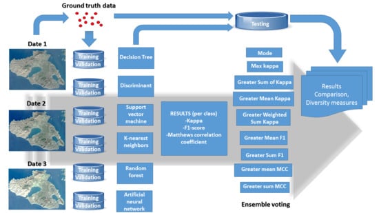
The methodology consists of three stages: the ground truth data collection, the classification by applying six base classifiers including the estimation of accuracy and diversity metrics, and finally the application of nine ensemble voting methods.

2.2.1. Ground Truth Data Collection

As used by several other studies [55,56,57] the input dataset was created by visual interpretation of Google Earth’s very high resolution images among with auxiliary data collected during field trips and a land cover map that was previously produced on the basis of a Worldview-2 image. A total of 1,119 homogenous polygons were identified and outlined with a total area of 127.4 km² across the island (

Table 2. Number of pixels per class and dataset.

Class	Number of Polygons	Number of Training Dataset	Number of Testing Dataset	Total Samples
Olive grove	342	3203	797	4000
Oak forest	72	1309	327	1636
Brushwood	73	4254	1088	5342
Built up	107	984	257	1241
Pinus brutia	113	4257	1090	5347
Chesnut forest	31	778	178	956
Pinus nigra	20	349	82	431
Maquis-type shrubland	107	936	226	1162
Barren land	44	212	61	273
Grassland	127	1327	312	1639
Other broadleaves	8	234	50	284
Agricultural land	54	729	188	917
Aquatic bodies	21	1070	254	1324
Total	1119	19642	4910	24552

). Within these polygons, random points were created to extract the values from the 30 layers of the image composition. The next step was to randomly split the dataset into training and testing partitions based on the 80% and the 20% of the initial cases. The training dataset was used to train all base classifiers and was further randomly split into a secondary training and validation dataset including the 75% and the 25% respectively.

Figure 2 presents the multitemporal spectral responses per class. The data of Figure 2 reveals significant differences in the spectral signatures within the date range especially in the near infrared (NIR) region except for pine forest. Furthermore, these data also address the phenology stages of deciduous, i.e., chestnut trees and agricultural lands. The variation of chlorophyll content in vegetation results in a significant variation of reflectance especially in infrared bands. These variations cause different phenological patterns for each vegetation cover type. According to previous studies, the different phenologies as described by these spectral responses is expected to improve the classification accuracy values compared to a single-date image especially in study areas where crops and vegetation are the dominant land cover types [58].

2.2.2. Base Classifiers

On the basis of the literature, six base classifiers have been selected for the case study. A widely used non-parametric approach is the decision tree (DT) classifier characterized also by its intuitive simplicity [59]. Within DT the input data is recursively split, based on a set of rules, into smaller and more homogenous groups forming the branches of the tree until the end-nodes, which are the target values. In our case, these target nodes forming the leaves represent the classes. One of the major advantages of DT is that it does not have any prerequisites about input data distribution. Moreover, a good generalization can be achieved by pruning the DT that means to remove some branches or turning some branches into leaves. Therefore, pruning will increase the accuracy by avoiding overfitting [11,60].

Another widely used classification approach, which is based on Fisher’s score optimization, is the DIS [61]. DIS approaches has been extensively used in the classification of hyperspectral data, either the initial or modified methods [62,63,64]. One of the major drawbacks of DIS in hyperspectral classification is that these data are ill-posed when the number of data are less than the number of bands. In our case, our data are more than sufficient to avoid this phenomenon during the classification of a 30-dimension space.

A third method that we applied is the Support Vector Machine (SVM) which aims to find a hyperplane that separates categorical data in a high dimension space with the maximum possible margin between the hyperplane and the cases [65]. The cases that are closest to the hyperplane are called support vectors. However, in most cases, the classes are not linearly separable, hence a slack variable is included, and a kernel function is used to perform a non-linear mapping into the feature space. The most widely used kernels in remote sensing applications are the polynomials and radial basis functions (RBF) [11,66].

The forth approach was a k-Nearest Neighbor (KNN) classifier. This algorithm calculates the distances between an unclassified case and the nearest k training cases and classifies the unclassified case to the majority class of the nearest k training cases. The user can choose from a variety of distance metrics, however, the most widely used is the Euclidean Distance which can be applied either unweighted or with a weight [67].

The next applied classification method was the random forest (RF). The concept of DTs is expanded and enhanced through the RF algorithm. Multiple DTs are trained on the basis of a subset of the training data where each one is trained on the basis of its own random sample. A majority vote of all the DTs defines the final class of each case. One of the advantages is that RF does not make any assumption about the probability distribution of the input data [13]. A more detailed description of the RF algorithm in remote sensing applications can be found in [68,69,70].

Finally, we developed and applied an artificial neural network (ANN) classifier. ANNs have been very popular and have been extensively used in pattern recognition and in modeling complex problems. In the last 30 years, ANNs play a fundamental role in remote sensing land cover classification applications [71,72,73,74], while the new trend in the classification of very high resolution images are the convolutional neural networks (CNN) [75,76]. The CNNs have proven, in the last years, to be very powerful classifiers in image recognition, object detection, image segmentation, and instance segmentation [77]. However, CNNs are fundamentally based on spatial-contextual dependencies of the input data with the majority of them being trained on high resolution RGB images [78,79]. Opposite to patch-based CNNs, pixel-based CNNs have been developed. However, according to the literature, the common problems of pixel-based classification, i.e., the salt and pepper effect and the boundary fuzziness effect within the classification result are quite severe in CNN implementations [80]. Other disadvantages of CNNs are the higher processing time and resources. We believe that, for the pixel-based hard classification of the present multispectral and multitemporal approach, ANNs are more suitable given also the nature of the other base classifiers. ANNs are characterized by their architecture, their training algorithm, and their activation function. The most well-known and efficient type is the Multilayer Perceptron (MLP) with three layers: input, hidden, and output, while ANNs with one hidden layer are able to map any nonlinear function. Various gradient descent learning methods have been proposed.

The evaluation, comparison, and voting during the ensemble of the applied methods were based on the below metrics:

$$verall Accuracy \left(OA\right)=\frac{TP+TN}{TP+FP+TN+FN}$$

(1)

$$User’s accuracy \left(UA\right)=\frac{TP}{TP+FN}$$

(2)

$$Producer’s accuracy \left(PA\right)=\frac{TP}{TP+FP}$$

(3)

$$kappa=\frac{p_0-p_e}{1-p_e} with$$

(4)

$$p_0=\frac{TP+TN}{TP+TN+FP+FN} \mathrm{and}$$

(5)

$$p_e=\frac{\left(TP+FN\right)\times \left(TP+FP\right)+\left(FP+TN\right)\times \left(FN+TN\right)}{{\left(TP+TN+FP+FN\right)}^2}$$

(6)

$$F1-score=\frac{2\times TP}{2\times TP+FP+FN}$$

(7)

$$\mathrm{MCC}=\frac{TP\times TN-FP\times FN}{\sqrt{\left(TP+FP\right)\times \left(TP+FN\right)\times \left(TN+FP\right)\times \left(TN+FN\right)}}$$

(8)

where TP: true positive, TN: true negative, FP: false positive, and FN: false negative. The overall accuracy (OA) is a single and very basic summary measure of the probability of a case being correctly classified and is based on the sum of the diagonal elements of the confusion matrix. User’s accuracy (UA) and producer’s accuracy (PA) provide an accuracy performance for each class. UA is a performance measure of the credibility of the output map that is how well the map represents the actual cover types. On the other hand, PA measures the accuracy of how well the reference data is represented by the map. UA and PA are related with the commission and the omission errors respectively. The kappa coefficient on the other hand is a more advanced metric, which compares the observed accuracy against random chance. Opposite to OA, the kappa coefficient takes also into consideration the non-diagonal elements. Furthermore, the F1-score is a rather different measure of accuracy, defined as the weighted harmonic mean of both classification’s precision and recall. It balances the use of precision and recall and provides a more realistic measure of performance. Finally, the Matthews correlation coefficient (MCC) is a more balanced metric that takes into account all parts of the confusion matrix and can handle under-represented classes. Each classifier produced a contingency matrix presenting the classification results of its validation dataset and the corresponding accuracy metrics. It should be noticed that for the calculation of the kappa, F1, and MCC for each class, each confusion matrix was converted to multiple binary matrices based on the ‘one-vs-all’ scheme.

Moreover, four different diversity statistics were calculated on the basis of the results of the base classifiers to the testing datasets, as depicted by the following 2 × 2 table of the relationship between a pair of classifiers C_i and C_k (

Table 3. Relational table between a pair of classifiers.

	Ci Correct (1)	Ci Wrong (0)
Ck correct (1)	N11	N10
Ck wrong (0)	N01	N00

) [81].

Where N¹¹ is the correctly classified cases by both classifiers, N¹⁰ is the correctly classified cases by C_k classifier, N⁰¹ is the correctly classified cases by Ci classifier, and N⁰⁰ is the incorrectly classified cases by both classifiers. The diversity measures were the Q-statistic, the disagreement measure, the double-fault measure, and the inter-kappa statistic given by [36,81,82,83]:

$$Inter-kappa measure=\frac{2\left(N^{11}{N}^{00}-N^{01}{N}^{10}\right)}{\left(N^{11}+N^{10}\right)\left(N^{01}+N^{00}\right)+\left(N^{11}+N^{01}\right)\left(N^{10}+N^{00}\right)}$$

(9)

$$Q_{i,k} statistic=\frac{N^{11}{N}^{00}-N^{01}{N}^{10}}{N^{11}{N}^{00}+N^{01}{N}^{10}}$$

(10)

$$disagreement measure=\frac{N^{01}+N^{10}}{N^{11}+N^{10}+N^{01}+N^{00}}$$

(11)

$$double-fault measure=\frac{N^{00}}{N^{11}+N^{10}+N^{01}+N^{00}}$$

(12)

2.2.3. Ensemble Voting Methods

After obtaining results from the six classifiers, an ensemble classifier should be constructed in order to classify the 4,910 cases of the testing dataset. For each testing case, all the base classifiers provided a prediction, and we tested nine different voting schemes to further evaluate:

• ‘Mode’: This voting method selects the suggestion with greater frequency in the six suggestions. In the cases with equal frequency, it selects the one with the higher sum of kappa.
• ‘Max kappa’: This voting method selects the suggestion with greater kappa.
• ‘Greater Sum of Kappa’: This voting method selects the suggestion with the greater sum of kappa aggregated on the suggestions. Identical suggestions are summed up and then compared with all other kappa values.
• ‘Greater Mean Kappa’: This method selects the suggestion with greater average kappa per suggestion. Identical suggestions are averaged and then compared with all other suggestions.
• ‘Greater Weighted Sum Kappa’: This method calculates the weighted sum of kappa which is the multiplication of the sum of kappa over the frequency of each suggestion group. Then, it selects the suggestion with the greater weighted sum of kappa.
• ‘Greater mean F1’: This voting method evaluates the average F1-score per suggestion and selects the one with the greater average F1. After grouping suggestions, we estimate the average F1 by group and compare the results. The result will be the one with the one with greater average F1-score.
• ‘Greater sum F1’: This voting method selects the suggestion with a greater aggregation of F1. After grouping the suggestions, we calculate the summation of F1 per group and compare the results. The result will be the suggestion group with the greater sum of F1-score.
• ‘Greater mean MCC’: This voting method evaluates the average MCC per suggestion group and then selects the one with the greater “mean MCC”. After grouping the suggestions, we average their MCC value and compare the results. The result will be the suggestion group with the greater average MCC
• ‘Greater sum MCC’: This last voting method selects the suggestion with the greater average MCC. After grouping suggestions, we evaluate the summation of MCC per group before evaluating the result. The result will be the suggestion group with the greater sum of MCC.

For all the above voting methods, the metrics of kappa, F1, and MCC are the ones of the corresponding metrics calculated for each class of the validation dataset during the training phase. The final comparison and selection of the best voting method was based on the kappa value. It should be noticed that even if we have computed the OA, we did not use it during the ensemble phase. Due to the imbalanced input dataset, the overall accuracy does not have an adequate performance, thus we used the kappa, the F1-score, and the MCC.

The nine ensemble models were further statistically compared by applying McNemar’s test [84]. McNemar’s test has been widely used in comparison of classifiers performances [85]. All models were compared in pairs and the McNemar’s value was given by:

$${\mathrm{McNemar}}^{’}\mathrm{s} \mathrm{value}=\frac{{\left(\left|n_{01}-n_{10}\right|-1\right)}^2}{n_{01}+n_{10}}$$

(13)

where $n_{01}$ is the number of samples misclassified only by algorithm A and $n_{10}$ is the number of samples misclassified only by algorithm B. The null hypothesis is that both of the classification methods have the same error rate. McNemar’s test is based on a $x^2$ test with one degree of freedom, where the critical $x^2$ value with a 95% confidence interval and a 5% level of significance is 3.841. If the computed McNemar’s value for each pair is more than 3.841, then the null hypothesis is rejected, therefore, the two classification methods are significantly different.

The ArcGIS 10.2 [86] was used for the spatial processing and visualization of the data, the Matlab 2018a [87] for the base classifications, while the ensemble of the classifiers through the voting methods was carried out using R, including the packages caret, dplyr, and magrittr [88,89,90,91]. Figure 3 presents the overall workflow of the current research.

3. Results and Discussion

Each base classifier was carefully designed and trained under different settings. This section presents the training results of the base classifiers and the classification ensemble. A diversity analysis of the base classifiers and a significant test of the voting methods provide a more comprehensive view of the results.

3.1. Base Classifiers Training

For the training of the DT classifiers we tested 4, 10, and 100 as the maximum number of splits. The best results obtained with 100 maximum splits based on Gini’s diversity index. The SVM classifier was trained with three different kernels; linear, RBF, quadratic and cubic. The cubic kernel provided the best accuracy and was further analyzed. We are aware that our approach is a multiclass imbalanced problem. It was decided that the best approach was to apply a “one-vs-one” instead of “one-vs-all” coding scheme in order to reduce the effect of the imbalance problem [92,93]. At the same time, the kappa, UA, PA, F1, and MCC provide a better interpretation of accuracy in an imbalanced dataset opposed to the overall accuracy. For the KNN we tested 1, 10, 100 nearest neighbors and the best results were provided with 10 neighbors. During the training, we applied the Euclidean distance unweighted and with a weight, but the overall accuracy increased when we used as a weight the inverse square of the distance for each case. The RF model tested with 30, 40, 50, 70, and 100 trees. The final model included 30 trees based on overall accuracy. Finally, during ANN training we applied different architectures with one hidden layer with 16 to 35 hidden nodes. We also tested two gradient descent learning methods: the Levenberg Marquardt [94] and the scaled conjugate gradient [95]. Each network was trained 10 times with different random initial weights. The model with the best performance had 16 hidden nodes and was trained with a scaled conjugate gradient for 272 epochs.

The classification accuracy of each classifier was evaluated based on the confusion matrix of the validation dataset presented in

Table A1. Confusion matrix for the validation dataset during the training phase of the base classifiers for the decision tree (DT) model.

		Reference
		OG	OF	BW	BU	PB	CF	PN	MS	BL	GL	OB	AL	AB	Total	UA
Predicted	OG	617	82	23	0	10	0	1	9	0	46	0	1	0	789	0.78
	OF	47	178	1	0	1	8	2	30	0	5	14	4	0	290	0.61
	BW	39	0	1012	10	0	0	0	0	4	92	0	1	0	1158	0.87
	BU	4	2	2	225	0	0	0	1	9	1	0	1	0	245	0.92
	PB	33	2	0	0	1034	3	47	26	0	0	11	0	0	1156	0.89
	CF	1	16	0	0	2	164	0	35	0	0	10	0	0	228	0.72
	PN	3	0	0	0	13	0	32	10	0	0	2	0	0	60	0.53
	MS	5	29	0	0	3	12	5	119	0	0	6	0	0	179	0.66
	BL	0	0	0	9	0	0	0	0	41	0	0	0	0	50	0.82
	GL	51	16	26	1	0	2	0	0	0	177	0	7	0	280	0.63
	OB	1	0	0	0	2	5	0	3	0	0	13	1	0	25	0.52
	AL	0	2	0	1	0	0	0	1	0	10	2	167	0	183	0.91
	AB	0	0	0	0	0	0	0	0	0	0	0	0	267	267	1
	Total	801	327	1064	246	1065	194	87	234	54	331	58	182	267
	PA	0.77	0.54	0.95	0.91	0.97	0.85	0.37	0.51	0.76	0.53	0.22	0.92	1	OA = 0.82
	kappa	0.73	0.55	0.88	0.91	0.91	0.77	0.43	0.56	0.79	0.55	0.31	0.91	1	kappa = 0.79

,

Table A2. Confusion matrix for the validation dataset during the training phase of the base classifiers for the discriminant (DIS) model.

		Reference
		OG	OF	BW	BU	PB	CF	PN	MS	BL	GL	OB	AL	AB	Total	UA
Predicted	OG	674	63	9	1	3	0	0	8	0	17	0	0	0	775	0.87
	OF	17	171	0	0	0	9	0	20	0	3	13	5	0	238	0.72
	BW	32	1	967	10	0	0	0	0	6	42	0	0	0	1058	0.91
	BU	0	0	2	212	0	0	0	0	2	0	0	0	0	216	0.98
	PB	42	3	0	0	1053	0	44	31	0	1	18	0	0	1192	0.88
	CF	1	27	0	0	0	164	0	16	0	0	8	3	0	219	0.75
	PN	3	3	0	0	5	0	40	4	0	0	0	0	0	55	0.73
	MS	5	36	0	0	4	20	3	152	0	0	7	0	0	227	0.67
	BL	0	1	1	23	0	0	0	0	46	0	0	0	0	71	0.65
	GL	26	14	85	0	0	0	0	0	0	263	1	10	0	399	0.66
	OB	1	8	0	0	0	1	0	3	0	0	11	0	0	24	0.46
	AL	0	0	0	0	0	0	0	0	0	5	0	164	0	169	0.97
	AB	0	0	0	0	0	0	0	0	0	0	0	0	267	267	1
	Total	801	327	1064	246	1065	194	87	234	54	331	58	182	267
	PA	0.84	0.52	0.91	0.86	0.99	0.85	0.46	0.65	0.85	0.79	0.19	0.9	1	OA = 0.85
	kappa	0.83	0.58	0.89	0.91	0.91	0.79	0.56	0.64	0.73	0.7	0.26	0.93	1	kappa = 0.83

,

Table A3. Confusion matrix for the validation dataset during the training phase of the base classifiers for the support vector machine (SVM) model.

		Reference
		OG	OF	BW	BU	PB	CF	PN	MS	BL	GL	OB	AL	AB	Total	UA
Predicted	OG	743	35	8	0	4	0	0	7	0	13	1	1	0	812	0.92
	OF	23	259	0	0	0	4	0	15	0	2	1	1	0	305	0.85
	BW	5	1	1033	2	0	0	0	0	2	38	0	0	0	1081	0.96
	BU	3	0	0	242	0	0	0	0	5	0	0	0	0	250	0.97
	PB	6	0	0	0	1039	0	14	4	0	0	1	0	0	1064	0.98
	CF	0	2	0	0	0	172	0	13	0	0	5	0	0	192	0.9
	PN	1	0	0	0	12	0	72	2	0	0	1	0	0	88	0.82
	MS	3	24	0	0	7	16	1	186	0	0	10	1	0	248	0.75
	BL	0	0	0	2	0	0	0	0	47	0	0	0	0	49	0.96
	GL	17	6	23	0	0	0	0	0	0	275	1	6	0	328	0.84
	OB	0	0	0	0	3	2	0	7	0	0	37	0	0	49	0.76
	AL	0	0	0	0	0	0	0	0	0	3	1	173	0	177	0.98
	AB	0	0	0	0	0	0	0	0	0	0	0	0	267	267	1
	Total	801	327	1064	246	1065	194	87	234	54	331	58	182	267
	PA	0.93	0.79	0.97	0.98	0.98	0.89	0.83	0.79	0.87	0.83	0.64	0.95	1	OA = 0.93
	kappa	0.91	0.81	0.95	0.97	0.97	0.89	0.82	0.76	0.91	0.82	0.69	0.96	1	kappa = 0.91

,

Table A4. Confusion matrix for the validation dataset during the training phase of the base classifiers for the k-nearest neighbors (KNN) model.

		Reference
		OG	OF	BW	BU	PB	CF	PN	MS	BL	GL	OB	AL	AB	Total	UA
Predicted	OG	673	45	2	4	1	0	2	7	0	22	0	2	0	758	0.89
	OF	34	253	0	0	0	15	0	34	0	5	11	2	0	354	0.71
	BW	27	1	1038	15	0	0	0	0	3	50	0	0	0	1134	0.92
	BU	2	1	0	221	0	0	0	0	7	0	0	0	0	231	0.96
	PB	17	1	0	0	1047	0	24	13	0	2	9	0	2	1115	0.94
	CF	0	2	0	0	0	161	0	17	0	0	16	0	0	196	0.82
	PN	1	0	0	0	10	0	58	6	0	0	1	0	0	76	0.76
	MS	9	20	0	0	6	18	3	157	0	0	9	1	0	223	0.7
	BL	0	0	1	6	0	0	0	0	44	0	0	0	0	51	0.86
	GL	38	3	23	0	0	0	0	0	0	247	0	7	0	318	0.78
	OB	0	0	0	0	1	0	0	0	0	0	12	0	0	13	0.92
	AL	0	1	0	0	0	0	0	0	0	5	0	170	0	176	0.97
	AB	0	0	0	0	0	0	0	0	0	0	0	0	265	265	1
	Total	801	327	1064	246	1065	194	87	234	54	331	58	182	267
	PA	0.84	0.77	0.98	0.9	0.98	0.83	0.67	0.67	0.81	0.75	0.21	0.93	0.99	OA = 0.89
	kappa	0.84	0.72	0.93	0.92	0.95	0.82	0.71	0.67	0.84	0.74	0.34	0.95	1	Kappa = 0.87

,

Table A5. Confusion matrix for the validation dataset during the training phase of the base classifiers for the random forest (RF) model.

		Reference
		OG	OF	BW	BU	PB	CF	PN	MS	BL	GL	OB	AL	AB	Total	UA
Predicted	OG	724	54	8	0	4	0	3	14	0	38	1	1	724	847	0.85
	OF	22	235	0	0	0	7	0	18	0	3	3	2	22	290	0.81
	BW	21	1	1027	3	0	0	0	0	3	49	0	0	21	1104	0.93
	BU	4	1	2	242	0	0	0	0	12	0	0	2	4	263	0.92
	PB	10	0	0	0	1049	0	27	15	0	0	7	0	10	1108	0.95
	CF	1	6	0	0	0	173	0	14	0	0	15	0	1	209	0.83
	PN	1	0	0	0	3	0	57	3	0	0	1	0	1	65	0.88
	MS	5	24	0	0	8	14	0	169	0	0	10	0	5	230	0.73
	BL	0	0	0	1	0	0	0	0	39	0	0	0	0	40	0.97
	GL	13	4	27	0	0	0	0	0	0	234	0	8	13	286	0.82
	OB	0	0	0	0	1	0	0	1	0	0	20	0	0	22	0.91
	AL	0	2	0	0	0	0	0	0	0	7	1	169	0	179	0.94
	AB	0	0	0	0	0	0	0	0	0	0	0	0	0	267	1
	Total	801	327	1064	246	1065	194	87	234	54	331	58	182	801
	PA	0.9	0.72	0.97	0.98	0.98	0.89	0.66	0.72	0.72	0.71	0.34	0.93	0.9	OA = 0.90
	kappa	0.85	0.75	0.93	0.95	0.96	0.85	0.75	0.71	0.83	0.74	0.5	0.93	0.85	Kappa = 0.88

and

Table A6. Confusion matrix for the validation dataset during the training phase of the base classifiers for the artificial neural network (ANN) model.

		Reference
		OG	OF	BW	BU	PB	CF	PN	MS	BL	GL	OB	AL	AB	Total	UA
Predicted	OG	717	55	7	2	5	0	0	3	0	28	0	1	0	818	0.88
	OF	25	220	0	1	0	9	0	37	0	3	8	2	0	305	0.72
	BW	11	0	1044	3	0	0	0	0	3	43	0	2	0	1106	0.94
	BU	1	1	7	225	0	0	0	0	8	0	0	0	0	242	0.93
	PB	8	0	0	0	1034	0	39	12	0	0	13	0	0	1106	0.93
	CF	0	3	0	0	0	163	0	24	0	0	11	3	0	204	0.8
	PN	1	0	0	0	12	0	52	0	0	0	1	0	0	66	0.79
	MS	5	23	0	0	10	16	1	143	0	0	7	0	0	205	0.7
	BL	0	1	0	8	0	0	0	0	51	0	0	0	0	60	0.85
	GL	23	5	27	1	0	0	0	1	0	243	0	3	0	303	0.8
	OB	0	2	0	0	1	3	0	9	0	0	18	1	0	34	0.53
	AL	1	1	0	1	0	0	0	0	0	7	3	169	0	182	0.93
	AB	0	0	0	0	1	0	0	0	0	0	0	0	279	280	1
	Total	792	311	1085	241	1063	191	92	229	62	324	61	181	279
	PA	0.91	0.71	0.96	0.93	0.97	0.85	0.57	0.62	0.82	0.75	0.3	0.93	1	OA = 0.89
	kappa	0.87	0.7	0.94	0.93	0.94	0.82	0.65	0.64	0.83	0.76	0.37	0.93	1	Kappa = 0.87

.

Table 4. User accuracy (UA) and producer accuracy (PA) per class ¹ for the validation dataset during the training phase of the base classifiers ².

	DT		DIS		SVM		KNN		RF		ANN
	UA	PA	UA	PA	UA	PA	UA	PA	UA	PA	UA	PA
OG	0.77	0.78	0.84	0.87	0.93	0.92	0.84	0.89	0.90	0.85	0.91	0.88
OF	0.54	0.61	0.52	0.72	0.79	0.85	0.77	0.71	0.72	0.81	0.71	0.72
BW	0.95	0.87	0.91	0.91	0.97	0.96	0.98	0.92	0.97	0.93	0.96	0.94
BU	0.91	0.92	0.86	0.98	0.98	0.97	0.90	0.96	0.98	0.92	0.93	0.93
PB	0.97	0.89	0.99	0.88	0.98	0.98	0.98	0.94	0.98	0.95	0.97	0.93
CF	0.85	0.72	0.85	0.75	0.89	0.90	0.83	0.82	0.89	0.83	0.85	0.80
PN	0.37	0.53	0.46	0.73	0.83	0.82	0.67	0.76	0.66	0.88	0.57	0.79
MS	0.51	0.66	0.65	0.67	0.79	0.75	0.67	0.70	0.72	0.73	0.62	0.70
BL	0.76	0.82	0.85	0.65	0.87	0.96	0.81	0.86	0.72	0.97	0.82	0.85
GL	0.53	0.63	0.79	0.66	0.83	0.84	0.75	0.78	0.71	0.82	0.75	0.80
OB	0.22	0.52	0.19	0.46	0.64	0.76	0.21	0.92	0.34	0.91	0.30	0.53
AL	0.92	0.91	0.90	0.97	0.95	0.98	0.93	0.97	0.93	0.94	0.93	0.93
AB	1	1	1	1	1	1	0.99	1	1	1	1	1
Overall Accuracy	0.82		0.85		0.93		0.89		0.90		0.89

¹ With bold fonts the maximum UA and PA per class. OG: olive grove, OF: oak forest, BW: brushwood, BU: built up, PB: Pinus brutia, CF: chesnut forest, PN: Pinus nigra, MS: maquis-type shrubland, BL: barren land, GL: grassland, OB: other broadleaves, AL: agricultural land, AB: aquatic bodies. ² DT: decision tree, DIS: discriminant, SVM: support vector machine, KNN: k-nearest neighbors, RF: random forest, ANN: artificial neural network.

shows the user’s (UA), producer’s (PA) accuracy per class and the OA for each classifier while Figure 4 presents the heat map of UA and PA where the colors are normalized for each classifier. According to the results, the SVM outperformed all the classifiers according to the OA and the kappa (Figure 5). In most of the land cover classes, SVM presented the lower omission and commission errors while the DT and the DIS had the poorest performance with kappa 0.79 and 0.83, respectively. Aquatic bodies were almost perfectly classified by all classifiers, while brushwood, built up, Pinus brutia, and agricultural land classes also showed high accuracy. Figure 6 presents the diversity of UA and PA among all classifiers for each class. The base classifiers had significant different performances in omission error for other broadleaves, barren land, and grassland classes and different performances in the commission error for oak forest, Pinus nigra, and other broadleaves. It should be noticed that the UA of SVM for other broadleaves is an outlier, i.e., its value is more than 1.5 times the interquartile range above the upper quartile.

Results are consistent with what has been found in previous studies. Shang et al. [96] applied SVM, RF and AdaBoost for the classification over an Australian eucalyptus forest. According to their results all three machine-learning algorithms outperformed the results produced by DIS. DT and DIS methods have also shown a poor performance in the comparison for the classification of Sentinel-2 data where RF outperformed followed by SVM and ANN [97]. However, the diversity of the results in the literature, reveals that the applied methods are data-driven and depended on the classification scheme, the number of training data and the type input data i.e. whether only the bands are taken into account or vegetation indices and other auxiliary data are used [19].

3.2. Classification Ensemble

During the ensemble, we tested the nine voting methods and the base classifiers with the testing dataset. Figure 7 shows the k coefficient for the base classifiers and the voting methods applied in the testing dataset. According to the results, the SVM outperforms not only the base classifiers but also all the voting methods. However, all the voting methods based on sums as well as the method based on the majority of the votes performed better that all the rest of the base classifiers. It is worth mentioning that DT present the lower k among all classifiers, while DIS has the second to last performance.

Table 5. Kappa coefficient per class ¹ of all classifiers ² for the testing dataset.

	OG	OF	BW	BU	PB	CF	PN	MS	BL	GL	OB	AL	AB
DT	0.72	0.61	0.88	0.90	0.93	0.81	0.40	0.59	0.77	0.54	0.32	0.91	1.00
DIS	0.84	0.59	0.88	0.91	0.91	0.75	0.51	0.64	0.75	0.62	0.05	0.93	1.00
SVM	0.90	0.83	0.94	0.95	0.97	0.87	0.83	0.80	0.87	0.78	0.68	0.99	1.00
KNN	0.84	0.74	0.91	0.89	0.95	0.82	0.72	0.70	0.78	0.71	0.35	0.98	1.00
RF	0.84	0.75	0.93	0.94	0.96	0.84	0.73	0.72	0.84	0.72	0.54	0.96	1.00
ANN	0.86	0.71	0.92	0.94	0.95	0.82	0.53	0.69	0.86	0.70	0.33	0.95	1.00
Mode	0.87	0.76	0.93	0.96	0.95	0.85	0.68	0.74	0.85	0.73	0.40	0.96	1.00
MaxK	0.82	0.74	0.91	0.94	0.90	0.80	0.42	0.69	0.75	0.58	0.00	0.93	1.00
GSK	0.87	0.76	0.93	0.96	0.95	0.84	0.68	0.74	0.85	0.73	0.30	0.96	1.00
GMK	0.79	0.64	0.90	0.93	0.90	0.75	0.42	0.68	0.72	0.58	0.04	0.93	1.00
GWSK	0.87	0.76	0.93	0.96	0.95	0.85	0.68	0.74	0.85	0.73	0.40	0.96	1.00
GMF1	0.78	0.63	0.89	0.89	0.90	0.75	0.40	0.68	0.72	0.54	0.04	0.93	1.00
GSF1	0.87	0.76	0.93	0.96	0.95	0.84	0.68	0.74	0.85	0.73	0.30	0.96	1.00
GMMCC	0.79	0.64	0.90	0.93	0.90	0.75	0.42	0.68	0.73	0.59	0.04	0.93	1.00
GSMCC	0.87	0.76	0.93	0.96	0.95	0.84	0.68	0.74	0.85	0.73	0.35	0.96	1.00

¹ With bold fonts the maximum kappa per class. ² Mode: mode, maxK: max kappa, GSK: greater sum of kappa, GMK: greater mean kappa, GWSK: greater weighted sum kappa, GMF1: greater mean F1, GSF1: greater sum F1, GMMCC: greater mean MCC, GSMCC: greater sumMCC.

presents the kappa coefficient per class for each classifier for the testing dataset, while the Figure 8 presents the corresponding heatmap. It is observed that SVM shows a better performance in almost all classes. The voting methods based on sums and the majority of the votes performed slightly better in the built-up class. The confusion matrices of the testing dataset of the best classifier and the best ensemble methods are presented in

Table A7. Confusion matrix for the test dataset of the SVM model.

		Reference
		OG	OF	BW	BU	PB	CF	PN	MS	BL	GL	OB	AL	AB	Total	UA
Predicted	OG	740	35	7	2	6	1	0	10	1	21	0	1	0	824	0.90
	OF	27	271	0	1	0	2	0	9	0	5	1	0	0	316	0.86
	BW	8	0	1031	3	0	0	0	0	0	34	0	0	0	1076	0.96
	BU	0	0	1	246	0	0	0	0	10	0	0	0	0	257	0.96
	PB	2	0	0	0	1062	0	15	3	0	1	4	0	0	1087	0.98
	CF	0	1	0	0	0	152	0	11	0	0	5	0	0	169	0.90
	PN	0	0	0	0	10	0	66	0	0	0	0	0	0	76	0.87
	MS	4	12	0	0	9	17	1	189	0	1	6	0	0	239	0.79
	BL	0	0	0	4	0	0	0	0	50	0	0	0	0	54	0.93
	GL	15	4	49	1	0	0	0	0	0	250	0	2	0	321	0.78
	OB	1	2	0	0	3	6	0	4	0	0	34	0	0	50	0.68
	AL	0	2	0	0	0	0	0	0	0	0	0	185	0	187	0.99
	AB	0	0	0	0	0	0	0	0	0	0	0	0	254	254	1
	Total	797	327	1088	257	1090	178	82	226	61	312	50	188	254	4910
	PA	0.93	0.83	0.95	0.96	0.97	0.85	0.80	0.84	0.82	0.80	0.68	0.98	1	OA = 0.92
	kappa	0.9	0.83	0.94	0.95	0.97	0.87	0.83	0.8	0.87	0.78	0.68	0.99	1	Kappa = 0.91

,

Table A8. Confusion matrix for the test dataset of the Greater Weighted Sum of Kappa ensemble model.

		Reference
		OG	OF	BW	BU	PB	CF	PN	MS	BL	GL	OB	AL	AB	Total	UA
Predicted	OG	727	42	5	3	4	0	1	7	1	25	0	0	0	815	0.89
	OF	20	244	0	0	0	2	0	13	0	6	5	0	0	290	0.84
	BW	15	0	1037	3	0	0	0	0	3	35	0	1	0	1094	0.95
	BU	0	0	1	248	0	0	0	0	8	0	0	0	0	257	0.96
	PB	6	0	0	0	1074	0	26	9	0	2	7	0	0	1124	0.96
	CF	0	3	0	0	0	159	0	16	0	0	12	0	0	190	0.84
	PN	0	0	0	0	1	0	55	0	0	0	0	0	0	56	0.98
	MS	9	28	0	0	10	17	0	179	0	1	5	0	0	249	0.72
	BL	0	0	1	2	0	0	0	0	49	0	0	0	0	52	0.94
	GL	20	7	44	1	0	0	0	0	0	241	0	4	0	317	0.76
	OB	0	1	0	0	1	0	0	2	0	0	19	0	0	23	0.83
	AL	0	2	0	0	0	0	0	0	0	2	2	183	0	189	0.97
	AB	0	0	0	0	0	0	0	0	0	0	0	0	254	254	1
	Total	797	327	1088	257	1090	178	82	226	61	312	50	188	254	4910
	PA	0.91	0.75	0.95	0.96	0.99	0.89	0.67	0.79	0.80	0.77	0.38	0.97	1	OA = 0.91
	kappa	0.87	0.76	0.93	0.96	0.95	0.85	0.68	0.74	0.85	0.73	0.40	0.96	1	Kappa = 0.89

and

Table A9. Confusion matrix for the test dataset of the Mode ensemble model.

		Reference
		OG	OF	BW	BU	PB	CF	PN	MS	BL	GL	OB	AL	AB	Total	UA
Predicted	OG	727	42	5	3	4	0	1	7	1	25	0	0	0	815	0.89
	OF	20	244	0	0	0	2	0	13	0	6	5	0	0	290	0.84
	BW	15	0	1037	3	0	0	0	0	3	35	0	1	0	1094	0.95
	BU	0	0	1	248	0	0	0	0	8	0	0	0	0	257	0.96
	PB	6	0	0	0	1074	0	26	9	0	2	7	0	0	1124	0.96
	CF	0	3	0	0	0	159	0	16	0	0	12	0	0	190	0.84
	PN	0	0	0	0	1	0	55	0	0	0	0	0	0	56	0.98
	MS	9	28	0	0	10	17	0	179	0	1	5	0	0	249	0.72
	BL	0	0	1	2	0	0	0	0	49	0	0	0	0	52	0.94
	GL	20	7	44	1	0	0	0	0	0	241	0	4	0	317	0.76
	OB	0	1	0	0	1	0	0	2	0	0	19	0	0	23	0.83
	AL	0	2	0	0	0	0	0	0	0	2	2	183	0	189	0.97
	AB	0	0	0	0	0	0	0	0	0	0	0	0	254	254	1
	Total	797	327	1088	257	1090	178	82	226	61	312	50	188	254	4910
	PA	0.89	0.84	0.95	0.96	0.96	0.84	0.98	0.72	0.94	0.76	0.83	0.97	1	OA = 0.91
	kappa	0.87	0.76	0.93	0.96	0.95	0.85	0.68	0.74	0.85	0.73	0.40	0.96	1	Kappa = 0.89

. According to the results, it is evident that the combination of the classifiers does not provide always a better performance compared to the base classifiers. In a crop classification study in a fragmented arable landscape by Salas et al. [98], the authors concluded that when no classifier is clearly performing better than the others then an ensemble approach can be the best alternative. In our case SVM, RF, ANN, and KNN show a similar performance, however the SVM method performs better than all the applied voting methods. Therefore, a diversity study was applied in order to identify any potential dissimilar performance between SVM and the other base classifiers.

Table 6. Diversity measures for all the possible pairs of base classifiers (a) inter-kappa measure, (b) Q-statistic, (c) disagreement measure, and (d) double-fault measure.

	DT	DIS	SVM	KNN	RF	DT	DIS	SVM	KNN	RF
DIS	0.523	-	-	-	-	0.895	-	-	-	-
SVM	0.356	0.367	-	-	-	0.870	0.871	-	-	-
KNN	0.540	0.483	0.477	-	-	0.930	0.896	0.924	-	-
RF	0.583	0.515	0.509	0.671	-	0.962	0.926	0.935	0.971	-
ANN	0.511	0.602	0.493	0.532	0.574	0.915	0.951	0.931	0.922	0.943
			(a)					(b)
	DT	DIS	SVM	KNN	RF	DT	DIS	SVM	KNN	RF
DIS	0.130	-	-	-	-	0.097	-	-	-	-
SVM	0.142	0.132	-	-	-	0.052	0.050	-	-	-
KNN	0.113	0.122	0.092	-	-	0.086	0.075	0.051	-	-
RF	0.099	0.110	0.081	0.064	-	0.087	0.074	0.050	0.078	-
ANN	0.120	0.094	0.089	0.096	0.083	0.083	0.089	0.052	0.068	0.068
			(c)					(d)

presents the result of the four diversity statistics for all the possible pairs of the base classifiers for the testing dataset. According to the inter-kappa measure (Table 6a), all classifiers show a moderate agreement between them, except for SVM, which shows a fair agreement with DT and DIS and a moderate agreement with the rest of the classifiers. The high values of the Q-statistic (Table 6b) and the low values of the disagreement measure (Table 6c) suggest that there is not any significant diversity of the classifiers. The same conclusion results from the double-fault measure (Table 6d). However, from Figure 9, it is evident that the SVM presents a diverse performance especially based on the double-fault and the inter-kappa measures (Figure 9a,d). SVM’s double-fault measures are tightly grouped while the values are quite low. Furthermore, the group of SVM’s inter-kappa measures are lower, while the rest of the classifiers have a similar performance. Therefore, from the combination of the classification performance of the base classifiers with the diversity results is revealed that a voting method does not provide a better performance when a base classifier has a small but identifiable better performance than the rest of the classifiers.

On the other hand, McNemar’s test of the ensemble methods showed that the voting method based on greater kappa is significantly different from the rest of the voting methods (

Table 7. McNemar’s test x² values for pair comparisons of ensemble methods ¹.

	MaxK	GSK	GMK	GWSK	GMF1	GSF1	GMMCC	GSMCC
Mode	13.483	0	1.028	0	1.125	0	1.936	0
MaxK	-	13.483	36.860	13.483	36.423	14.095	40.830	13.483
GSK	-	-	1.028	0	1.125	0	1.954	0
GMK	-	-	-	1.028	0	0.921	3.063	1.028
GWSK	-	-	-	-	1.125	0	1.954	0
GMF1	-	-	-	-	-	1.028	1.895	1.125
GSF1	-	-	-	-	-	-	1.787	0
GMMCC	-	-	-	-	-	-	-	1.936

¹ With bold fonts the McNemar’s test x² values greater than value 3.84.

). More specifically, the $x^2$ exceeds the critical $x^2$ value of 3.84 and thus ‘MaxK’ is statistically significant at a 95% confidence interval for all the pair comparisons. Interestingly, the rest of the comparisons revealed that the null hypothesis cannot be rejected according to McNemar’s test, hence the difference in accuracy between the ensemble methods is not statistically significant.

4. Conclusions

This work illustrates the potential use of a number of classifiers on identifying land cover types. The land cover type mapping is essential for the land management of the Mediterranean ecosystems. Long-term human activities along with geographic and climatic conditions have created a heterogeneous fragmented ecosystem that changes rapidly [99]. One of the main disturbances of Mediterranean ecosystems are wildfires. Land cover type mapping provides valuable information, i.e., vegetative fuel and socioeconomic inputs in wildfire risk assessment [100,101]. Furthermore, through remote sensing classification we can identify the change detection, possible land degradations and empower ecosystem monitoring [102,103].

An ensemble approach with nine voting methods has been developed for increased accuracy over classification algorithms using multi-temporal Sentinel-2 data from a mixed Mediterranean ecosystem. Each base classifier was trained with its own dataset in order to create the accuracy metrics that were used within the voting methods. All the base classifiers and the ensemble methods were applied to an unseen testing dataset. The result shows that the combination of multiple classifiers based on the examined voting schemes does not always provide a better performance in land cover classification. The SVM algorithm outperformed all the classifiers and was proven as the most accurate approach especially for this quite unbalanced dataset.

The diversity measures can explain the outperformance of SVM. The double-fault measure clearly shows that SVM significantly differs from the rest of the classifiers. Therefore, diversity measures should be thoroughly examined before building an ensemble method. The diversity metrics can be evidence in identifying possible overperformance within base classifiers hence an ensemble may not be always necessary. On the other hand, possible underperformances can be identified leading to the exclusion of some base classifiers. To sum up, our voting methods were influenced by the number of classifiers with a lower performance opposed to SVM. Hence, the accuracy of the ensembles are lower than the best base classifier, probably due to the ‘curse of conflict’ problem [104].

Potential further improvements of this methodology should include the incorporation of additional base algorithms and more ensemble methods. Moreover, opposed to pixel-based approaches, ensembles of segmentation approaches can be explored including traditional segmentation algorithms and CNNs. An interesting potential improvement of this work should be the comparison of multiple Mediterranean areas based on the very same ensemble of algorithms. Nevertheless, this work has proven that contemporary computational approaches along with advanced algorithmic measures show potential for land cover classification of unbalanced data.

References

- Shen, H.; Lin, Y.; Tian, Q.; Xu, K.; Jiao, J. A comparison of multiple classifier combinations using different voting-weights for remote sensing image classification. Int. J. Remote Sens. 2018, 39, 3705–3722. [Google Scholar] [CrossRef]
- Maulik, U.; Chakraborty, D. Remote Sensing Image Classification: A survey of support-vector-machine-based advanced techniques. IEEE Geosci. Remote Sens. Mag. 2017, 5, 33–52. [Google Scholar] [CrossRef]
- Fathizad, H.; Hakimzadeh Ardakani, M.A.; Mehrjardi, R.T.; Sodaiezadeh, H. Evaluating desertification using remote sensing technique and object-oriented classification algorithm in the Iranian central desert. J. Afr. Earth Sci. 2018, 145, 115–130. [Google Scholar] [CrossRef]
- Gómez, C.; White, J.C.; Wulder, M.A. Optical remotely sensed time series data for land cover classification: A review. ISPRS J. Photogramm. Remote Sens. 2016, 116, 55–72. [Google Scholar] [CrossRef] [Green Version]
- Chen, K.S.; Tzeng, Y.C.; Chen, C.F.; Kao, W.L.; Ni, C.L. Classification of multispectral imagery using dynamic learning neural network. In Proceedings of the IGARSS ’93—IEEE International Geoscience and Remote Sensing Symposium, Tokyo, Japan, 18–21 August 2013; IEEE: Piscataway, NJ, USA, 1994; pp. 896–898. [Google Scholar]
- Lawrence, R. Classification of remotely sensed imagery using stochastic gradient boosting as a refinement of classification tree analysis. Remote Sens. Environ. 2004, 90, 331–336. [Google Scholar] [CrossRef]
- Sohn, Y.; Rebello, N.S. Supervised and unsupervised spectral angle classifiers. Photogramm. Eng. Remote Sens. 2002, 68, 1271–1280. [Google Scholar]
- Strahler, A.H. The use of prior probabilities in maximum likelihood classification of remotely sensed data. Remote Sens. Environ. 1980, 10, 135–163. [Google Scholar] [CrossRef]
- Foody, G.M.; Mathur, A. A relative evaluation of multiclass image classification by support vector machines. IEEE Trans. Geosci. Remote Sens. 2004, 42, 1335–1343. [Google Scholar] [CrossRef] [Green Version]
- Collins, M.J.; Dymond, C.; Johnson, E.A. Mapping subalpine forest types using networks of nearest neighbour classifiers. Int. J. Remote Sens. 2004, 25, 1701–1721. [Google Scholar] [CrossRef]
- Maxwell, A.E.; Warner, T.A.; Fang, F. Implementation of machine-learning classification in remote sensing: An applied review. Int. J. Remote Sens. 2018, 39, 2784–2817. [Google Scholar] [CrossRef] [Green Version]
- Qian, Y.; Zhou, W.; Yan, J.; Li, W.; Han, L. Comparing Machine Learning Classifiers for Object-Based Land Cover Classification Using Very High Resolution Imagery. Remote Sens. 2014, 7, 153–168. [Google Scholar] [CrossRef]
- Ghamisi, P.; Plaza, J.; Chen, Y.; Li, J.; Plaza, A.J. Advanced Spectral Classifiers for Hyperspectral Images: A review. IEEE Geosci. Remote Sens. Mag. 2017, 5, 8–32. [Google Scholar] [CrossRef] [Green Version]
- Ballanti, L.; Blesius, L.; Hines, E.; Kruse, B. Tree Species Classification Using Hyperspectral Imagery: A Comparison of Two Classifiers. Remote Sens. 2016, 8, 445. [Google Scholar] [CrossRef] [Green Version]
- Seetha, M.; Muralikrishna, I.V.; Deekshatulu, B.L.; Malleswari, B.L.; Hegde, P. Artificial Neural Networks and Other Methods of Image Classification. Theor. Appl. Inf. Technol. 2008, 4, 1039–1053. [Google Scholar]
- Thanh Noi, P.; Kappas, M. Comparison of Random Forest, k-Nearest Neighbor, and Support Vector Machine Classifiers for Land Cover Classification Using Sentinel-2 Imagery. Sensors 2017, 18, 18. [Google Scholar] [CrossRef] [PubMed] [Green Version]
- Huang, C.; Davis, L.S.; Townshend, J.R.G. An assessment of support vector machines for land cover classification. Int. J. Remote Sens. 2002, 23, 725–749. [Google Scholar] [CrossRef]
- Lapini, A.; Pettinato, S.; Santi, E.; Paloscia, S.; Fontanelli, G.; Garzelli, A. Comparison of Machine Learning Methods Applied to SAR Images for Forest Classification in Mediterranean Areas. Remote Sens. 2020, 12, 369. [Google Scholar] [CrossRef] [Green Version]
- Ge, G.; Shi, Z.; Zhu, Y.; Yang, X.; Hao, Y. Land use/cover classification in an arid desert-oasis mosaic landscape of China using remote sensed imagery: Performance assessment of four machine learning algorithms. Glob. Ecol. Conserv. 2020, 22, e00971. [Google Scholar] [CrossRef]
- Dang, V.-H.; Hoang, N.-D.; Nguyen, L.-M.-D.; Bui, D.T.; Samui, P. A Novel GIS-Based Random Forest Machine Algorithm for the Spatial Prediction of Shallow Landslide Susceptibility. Forests 2020, 11, 118. [Google Scholar] [CrossRef] [Green Version]
- Abdi, A.M. Land cover and land use classification performance of machine learning algorithms in a boreal landscape using Sentinel-2 data. GISci. Remote Sens. 2020, 57, 1–20. [Google Scholar] [CrossRef] [Green Version]
- Tonbul, H.; Colkesen, I.; Kavzoglu, T. Classification of poplar trees with object-based ensemble learning algorithms using Sentinel-2A imagery. J. Geod. Sci. 2020, 10, 14–22. [Google Scholar] [CrossRef]
- Langley, S.K.; Cheshire, H.M.; Humes, K.S. A comparison of single date and multitemporal satellite image classifications in a semi-arid grassland. J. Arid Environ. 2001, 49, 401–411. [Google Scholar] [CrossRef]
- Yuan, F.; Sawaya, K.E.; Loeffelholz, B.C.; Bauer, M.E. Land cover classification and change analysis of the Twin Cities (Minnesota) Metropolitan Area by multitemporal Landsat remote sensing. Remote Sens. Environ. 2005, 98, 317–328. [Google Scholar] [CrossRef]
- Hütt, C.; Koppe, W.; Miao, Y.; Bareth, G. Best Accuracy Land Use/Land Cover (LULC) Classification to Derive Crop Types Using Multitemporal, Multisensor, and Multi-Polarization SAR Satellite Images. Remote Sens. 2016, 8, 684. [Google Scholar] [CrossRef] [Green Version]
- Eisavi, V.; Homayouni, S.; Yazdi, A.M.; Alimohammadi, A. Land cover mapping based on random forest classification of multitemporal spectral and thermal images. Environ. Monit. Assess. 2015, 187, 291. [Google Scholar] [CrossRef] [PubMed]
- Tigges, J.; Lakes, T.; Hostert, P. Urban vegetation classification: Benefits of multitemporal RapidEye satellite data. Remote Sens. Environ. 2013, 136, 66–75. [Google Scholar] [CrossRef]
- Alcantara, C.; Kuemmerle, T.; Prishchepov, A.V.; Radeloff, V.C. Mapping abandoned agriculture with multi-temporal MODIS satellite data. Remote Sens. Environ. 2012, 124, 334–347. [Google Scholar] [CrossRef]
- Key, T. A Comparison of Multispectral and Multitemporal Information in High Spatial Resolution Imagery for Classification of Individual Tree Species in a Temperate Hardwood Forest. Remote Sens. Environ. 2001, 75, 100–112. [Google Scholar] [CrossRef]
- Kamusoko, C. Image Classification. In Remote Sensing Image Classification in R; Springer: Singapore, 2019; pp. 81–153. [Google Scholar]
- Rujoiu-Mare, M.-R.; Olariu, B.; Mihai, B.-A.; Nistor, C.; Săvulescu, I. Land cover classification in Romanian Carpathians and Subcarpathians using multi-date Sentinel-2 remote sensing imagery. Eur. J. Remote Sens. 2017, 50, 496–508. [Google Scholar] [CrossRef] [Green Version]
- Sharma, A.; Liu, X.; Yang, X. Land cover classification from multi-temporal, multi-spectral remotely sensed imagery using patch-based recurrent neural networks. Neural Netw. 2018, 105, 346–355. [Google Scholar] [CrossRef] [Green Version]
- Pal, M.; Mather, P.M. A comparison of decision tree and backpropagation neural network classifiers for land use classification. In Proceedings of the International Geoscience and Remote Sensing Symposium (IGARSS), Toronto, ON, Canada, 24–28 June 2002. [Google Scholar]
- Rogan, J.; Franklin, J.; Stow, D.; Miller, J.; Woodcock, C.; Roberts, D. Mapping land-cover modifications over large areas: A comparison of machine learning algorithms. Remote Sens. Environ. 2008, 112, 2272–2283. [Google Scholar] [CrossRef]
- Pal, M.; Mather, P.M. Support vector machines for classification in remote sensing. Int. J. Remote Sens. 2005, 26, 1007–1011. [Google Scholar] [CrossRef]
- Du, P.; Xia, J.; Zhang, W.; Tan, K.; Liu, Y.; Liu, S. Multiple Classifier System for Remote Sensing Image Classification: A Review. Sensors 2012, 12, 4764–4792. [Google Scholar] [CrossRef]
- Briem, G.J.; Benediktsson, J.A.; Sveinsson, J.R. Multiple classifiers applied to multisource remote sensing data. IEEE Trans. Geosci. Remote Sens. 2002, 40, 2291–2299. [Google Scholar] [CrossRef] [Green Version]
- Aguilar, R.; Zurita-Milla, R.; Izquierdo-Verdiguier, E.; de By, R.A. A Cloud-Based Multi-Temporal Ensemble Classifier to Map Smallholder Farming Systems. Remote Sens. 2018, 10, 729. [Google Scholar] [CrossRef] [Green Version]
- Foody, G.M.; Boyd, D.S.; Sanchez-Hernandez, C. Mapping a specific class with an ensemble of classifiers. Int. J. Remote Sens. 2007, 28, 1733–1746. [Google Scholar] [CrossRef]
- Lei, G.; Li, A.; Bian, J.; Yan, H.; Zhang, L.; Zhang, Z.; Nan, X. OIC-MCE: A Practical Land Cover Mapping Approach for Limited Samples Based on Multiple Classifier Ensemble and Iterative Classification. Remote Sens. 2020, 12, 987. [Google Scholar] [CrossRef] [Green Version]
- Amani, M.; Salehi, B.; Mahdavi, S.; Brisco, B.; Shehata, M. A Multiple Classifier System to improve mapping complex land covers: A case study of wetland classification using SAR data in Newfoundland, Canada. Int. J. Remote Sens. 2018, 39, 7370–7383. [Google Scholar] [CrossRef]
- Doan, H.T.X.; Foody, G.M. Increasing soft classification accuracy through the use of an ensemble of classifiers. Int. J. Remote Sens. 2007, 28, 4609–4623. [Google Scholar] [CrossRef]
- Giacinto, G.; Roli, F. Ensembles of Neural Networks for Soft Classification of Remote Sensing Images. In Proceedings of the European Symposium on Intelligent Techniques, European Network for Fuzzy Logic and Uncertainty Modelling in Information Technology, Bari, Italy, 20–21 March 1997; pp. 166–170. [Google Scholar]
- Drucker, H.; Cortes, C.; Jackel, L.D.; LeCun, Y.; Vapnik, V. Boosting and Other Ensemble Methods. Neural Comput. 1994, 6, 1289–1301. [Google Scholar] [CrossRef]
- Breiman, L. Bagging predictors. Mach. Learn. 1996, 24, 123–140. [Google Scholar] [CrossRef] [Green Version]
- Pal, M. Ensemble of support vector machines for land cover classification. Int. J. Remote Sens. 2008, 29, 3043–3049. [Google Scholar] [CrossRef]
- Pal, M. Ensemble Learning with Decision Tree for Remote Sensing Classification. World Acad. Sci. Eng. Technol. 2007, 36, 258–260. [Google Scholar]
- Battiti, R.; Colla, A.M. Democracy in neural nets: Voting schemes for classification. Neural Netw. 1994, 7, 691–707. [Google Scholar] [CrossRef]
- Oza, N.C.; Tumer, K. Classifier ensembles: Select real-world applications. Inf. Fusion 2008, 9, 4–20. [Google Scholar] [CrossRef]
- Puletti, N.; Chianucci, F.; Castaldi, C. Use of Sentinel-2 for forest classification in Mediterranean environments. Ann. Silvic. Res. 2018, 42, 32–38. [Google Scholar]
- Chatziantoniou, A.; Psomiadis, E.; Petropoulos, G. Co-Orbital Sentinel 1 and 2 for LULC Mapping with Emphasis on Wetlands in a Mediterranean Setting Based on Machine Learning. Remote Sens. 2017, 9, 1259. [Google Scholar] [CrossRef] [Green Version]
- Henderson, M.; Kalabokidis, K.; Marmaras, E.; Konstantinidis, P.; Marangudakis, M. Fire and society: A comparative analysis of wildfire in Greece and the United States. Hum. Ecol. Rev. 2005, 12, 169–182. [Google Scholar]
- ESA Copernicus Open Access Hub. Available online: https://scihub.copernicus.eu/ (accessed on 10 February 2020).
- Hill, R.A.; Wilson, A.K.; George, M.; Hinsley, S.A. Mapping tree species in temperate deciduous woodland using time-series multi-spectral data. Appl. Veg. Sci. 2010, 13, 86–99. [Google Scholar] [CrossRef]
- Guirado, E.; Tabik, S.; Alcaraz-Segura, D.; Cabello, J.; Herrera, F. Deep-learning Versus OBIA for Scattered Shrub Detection with Google Earth Imagery: Ziziphus lotus as Case Study. Remote Sens. 2017, 9, 1220. [Google Scholar] [CrossRef] [Green Version]
- Li, Q.; Qiu, C.; Ma, L.; Schmitt, M.; Zhu, X.X. Mapping the Land Cover of Africa at 10 m Resolution from Multi-Source Remote Sensing Data with Google Earth Engine. Remote Sens. 2020, 12, 602. [Google Scholar] [CrossRef] [Green Version]
- Bwangoy, J.-R.B.; Hansen, M.C.; Roy, D.P.; De Grandi, G.; Justice, C.O. Wetland mapping in the Congo Basin using optical and radar remotely sensed data and derived topographical indices. Remote Sens. Environ. 2010, 114, 73–86. [Google Scholar] [CrossRef]
- Lu, D.; Weng, Q. A survey of image classification methods and techniques for improving classification performance. Int. J. Remote Sens. 2007, 28, 823–870. [Google Scholar] [CrossRef]
- Friedl, M.A.; Brodley, C.E. Decision tree classification of land cover from remotely sensed data. Remote Sens. Environ. 1997, 61, 399–409. [Google Scholar] [CrossRef]
- Almuallim, H. An efficient algorithm for optimal pruning of decision trees. Artif. Intell. 1996, 83, 347–362. [Google Scholar] [CrossRef] [Green Version]
- Aylmer Fisher FRS, R. Summary for Policymakers. In Climate Change 2013—The Physical Science Basis; Intergovernmental Panel on Climate Change, Ed.; Cambridge University Press: Cambridge, UK, 1936; pp. 1–30. ISBN 9788578110796. [Google Scholar]
- Bandos, T.V.; Bruzzone, L.; Camps-Valls, G. Classification of Hyperspectral Images with Regularized Linear Discriminant Analysis. IEEE Trans. Geosci. Remote Sens. 2009, 47, 862–873. [Google Scholar] [CrossRef]
- Feret, J.-B.; Asner, G.P. Tree Species Discrimination in Tropical Forests Using Airborne Imaging Spectroscopy. IEEE Trans. Geosci. Remote Sens. 2013, 51, 73–84. [Google Scholar] [CrossRef]
- Clark, M.; Roberts, D.; Clark, D. Hyperspectral discrimination of tropical rain forest tree species at leaf to crown scales. Remote Sens. Environ. 2005, 96, 375–398. [Google Scholar] [CrossRef]
- Cortes, C.; Vapnik, V. Support-vector networks. Mach. Learn. 1995, 20, 273–297. [Google Scholar] [CrossRef]
- Kavzoglu, T.; Colkesen, I. A kernel functions analysis for support vector machines for land cover classification. Int. J. Appl. Earth Obs. Geoinf. 2009, 11, 352–359. [Google Scholar] [CrossRef]
- Franco-Lopez, H.; Ek, A.R.; Bauer, M.E. Estimation and mapping of forest stand density, volume, and cover type using the k-nearest neighbors method. Remote Sens. Environ. 2001, 77, 251–274. [Google Scholar] [CrossRef]
- Gislason, P.O.; Benediktsson, J.A.; Sveinsson, J.R. Random Forests for land cover classification. Pattern Recognit. Lett. 2006, 27, 294–300. [Google Scholar] [CrossRef]
- Pal, M. Random forest classifier for remote sensing classification. Int. J. Remote Sens. 2005, 26, 217–222. [Google Scholar] [CrossRef]
- Belgiu, M.; Drăguţ, L. Random forest in remote sensing: A review of applications and future directions. ISPRS J. Photogramm. Remote Sens. 2016, 114, 24–31. [Google Scholar] [CrossRef]
- Mas, J.F.; Flores, J.J. The application of artificial neural networks to the analysis of remotely sensed data. Int. J. Remote Sens. 2008, 29, 617–663. [Google Scholar] [CrossRef]
- Atkinson, P.M.; Tatnall, A.R.L. Introduction Neural networks in remote sensing. Int. J. Remote Sens. 1997, 18, 699–709. [Google Scholar] [CrossRef]
- Yuan, H.; Van Der Wiele, C.; Khorram, S. An Automated Artificial Neural Network System for Land Use/Land Cover Classification from Landsat TM Imagery. Remote Sens. 2009, 1, 243–265. [Google Scholar] [CrossRef] [Green Version]
- Kavzoglu, T.; Mather, P.M. The use of backpropagating artificial neural networks in land cover classification. Int. J. Remote Sens. 2003, 24, 4907–4938. [Google Scholar] [CrossRef]
- Längkvist, M.; Kiselev, A.; Alirezaie, M.; Loutfi, A. Classification and Segmentation of Satellite Orthoimagery Using Convolutional Neural Networks. Remote Sens. 2016, 8, 329. [Google Scholar] [CrossRef] [Green Version]
- Pires de Lima, R.; Marfurt, K. Convolutional Neural Network for Remote-Sensing Scene Classification: Transfer Learning Analysis. Remote Sens. 2019, 12, 86. [Google Scholar] [CrossRef] [Green Version]
- Hoeser, T.; Kuenzer, C. Object Detection and Image Segmentation with Deep Learning on Earth Observation Data: A Review-Part I: Evolution and Recent Trends. Remote Sens. 2020, 12, 1667. [Google Scholar] [CrossRef]
- Zuo, Z.; Shuai, B.; Wang, G.; Liu, X.; Wang, X.; Wang, B.; Chen, Y. Convolutional recurrent neural networks: Learning spatial dependencies for image representation. In Proceedings of the 2015 IEEE Conference on Computer Vision and Pattern Recognition Workshops (CVPRW), Boston, MA, USA, 7–12 June 2015; IEEE: Piscataway, NJ, USA, 2015; pp. 18–26. [Google Scholar]
- Zhao, W.; Du, S. Spectral–Spatial Feature Extraction for Hyperspectral Image Classification: A Dimension Reduction and Deep Learning Approach. IEEE Trans. Geosci. Remote Sens. 2016, 54, 4544–4554. [Google Scholar] [CrossRef]
- Lv, X.; Ming, D.; Chen, Y.; Wang, M. Very high resolution remote sensing image classification with SEEDS-CNN and scale effect analysis for superpixel CNN classification. Int. J. Remote Sens. 2019, 40, 506–531. [Google Scholar] [CrossRef]
- Kuncheva, L.I.; Whitaker, C.J. Measures of diversity in classifier ensembles and their relationship with the ensemble accuracy. Mach. Learn. 2003, 51, 181–207. [Google Scholar] [CrossRef]
- Petrakos, M.; Atli Benediktsson, J.; Kanellopoulos, I. The effect of classifier agreement on the accuracy of the combined classifier in decision level fusion. IEEE Trans. Geosci. Remote Sens. 2001, 39, 2539–2546. [Google Scholar] [CrossRef] [Green Version]
- Thomas, G. Dietterich An Experimental Comparison of Three Methods for Constructing Ensembles of Decision Trees: Bagging, Boosting, and Randomization. Mach. Learn. 2000, 40, 139–157. [Google Scholar]
- Edwards, A.L. Note on the “correction for continuity” in testing the significance of the difference between correlated proportions. Psychometrika 1948, 13, 185–187. [Google Scholar] [CrossRef]
- Kavzoglu, T. Object-Oriented Random Forest for High Resolution Land Cover Mapping Using Quickbird-2 Imagery. In Handbook of Neural Computation; Academic Press: London, UK, 2017; ISBN 9780128113196. [Google Scholar]
- Environmental Systems Research Institute. ESRI ArcGIS Desktop: Release 10; Environmental Systems Research Institute: Redlands, CA, USA, 2013. [Google Scholar]
- The Mathworks Inc. The Mathworks Inc.: Massachusetts. 2018. Available online: https://www.Mathworks.com/Products/Matlab (accessed on 10 February 2020).
- R Development Core Team. R: A Language and Environment for Statistical Computing; R Development Core Team: Vienna, Austria, 2017. [Google Scholar]
- Wickham, H.; Francois, R. The Dplyr Package; R Core Team: Vienna, Austria, 2016. [Google Scholar]
- Bache, S.M.; Wickham, H. Package ‘magrittr’—A Forward-Pipe Operator for R. Available online: https://CRAN.R-project.org/package=magrittr (accessed on 10 February 2020).
- Kuhn, M. Building Predictive Models in R Using the caret Package. J. Stat. Softw. 2008, 28, 1–26. [Google Scholar] [CrossRef] [Green Version]
- Anthony, G.; Gregg, H.; Tshilidzi, M. Image classification using SVMs: One-Against-One vs One-against-All. In Proceedings of the 28th Asian Conference on Remote Sensing 2007, ACRS 2007, Kuala Lumpur, Malaysia, 12–16 November 2007. [Google Scholar]
- Daengduang, S.; Vateekul, P. Enhancing accuracy of multi-label classification by applying one-vs-one support vector machine. In Proceedings of the 2016 13th International Joint Conference on Computer Science and Software Engineering (JCSSE), Khon Kaen, Thailand, 13–15 July 2016; IEEE: Piscataway, NJ, USA, 2016; pp. 1–6. [Google Scholar]
- Marquardt, D.W. An Algorithm for Least-Squares Estimation of Nonlinear Parameters. J. Soc. Ind. Appl. Math. 1963, 11, 431–441. [Google Scholar] [CrossRef]
- Møller, M.F. A scaled conjugate gradient algorithm for fast supervised learning. Neural Netw. 1993, 6, 525–533. [Google Scholar] [CrossRef]
- Shang, X.; Chisholm, L.A. Classification of Australian Native Forest Species Using Hyperspectral Remote Sensing and Machine-Learning Classification Algorithms. IEEE J. Sel. Top. Appl. Earth Obs. Remote Sens. 2014, 7, 2481–2489. [Google Scholar] [CrossRef]
- Pirotti, F.; Sunar, F.; Piragnolo, M. Benchmark of machine learning methods for classification of a sentinel-2 image. ISPRS Int. Arch. Photogramm. Remote Sens. Spat. Inf. Sci. 2016, XLI-B7, 335–340. [Google Scholar] [CrossRef]
- Salas, E.A.L.; Subburayalu, S.K.; Slater, B.; Zhao, K.; Bhattacharya, B.; Tripathy, R.; Das, A.; Nigam, R.; Dave, R.; Parekh, P. Mapping crop types in fragmented arable landscapes using AVIRIS-NG imagery and limited field data. Int. J. Image Data Fusion 2020, 11, 33–56. [Google Scholar] [CrossRef]
- Gauquelin, T.; Michon, G.; Joffre, R.; Duponnois, R.; Génin, D.; Fady, B.; Bou Dagher-Kharrat, M.; Derridj, A.; Slimani, S.; Badri, W.; et al. Mediterranean forests, land use and climate change: A social-ecological perspective. Reg. Environ. Chang. 2018, 18, 623–636. [Google Scholar] [CrossRef]
- Vasilakos, C.; Kalabokidis, K.; Hatzopoulos, J.; Kallos, G.; Matsinos, Y. Integrating new methods and tools in fire danger rating. Int. J. Wildl. Fire 2007, 16, 306. [Google Scholar] [CrossRef]
- Vasilakos, C.; Kalabokidis, K.; Hatzopoulos, J.; Matsinos, I. Identifying wildland fire ignition factors through sensitivity analysis of a neural network. Nat. Hazards 2009, 50, 125–143. [Google Scholar] [CrossRef]
- Bajocco, S.; De Angelis, A.; Perini, L.; Ferrara, A.; Salvati, L. The impact of Land Use/Land Cover Changes on land degradation dynamics: A Mediterranean case study. Environ. Manag. 2012, 49, 980–989. [Google Scholar] [CrossRef]
- Otero, I.; Marull, J.; Tello, E.; Diana, G.L.; Pons, M.; Coll, F.; Boada, M. Land abandonment, landscape, and biodiversity: Questioning the restorative character of the forest transition in the Mediterranean. Ecol. Soc. 2015. [Google Scholar] [CrossRef] [Green Version]
- Song, C.; Pons, A.; Yen, K. Sieve: An Ensemble Algorithm Using Global Consensus for Binary Classification. AI 2020, 1, 16. [Google Scholar] [CrossRef]
Figure 1.
The Lesvos Island at the north-east Aegean sea (source of location panels: Esri).
Figure 2.
Spectral reflectance per class and per date.
Figure 3.
Workflow of the method followed for data classification and ensemble voting.
Figure 4.
User accuracy (UA) and producer accuracy (PA) heatmap for the validation dataset during the training phase of the base classifiers.
Figure 5.
Kappa coefficient per class for the validation dataset during the training phase of the base classifiers.
Figure 6.
Distribution of (a) user’s accuracy and (b) producer’s accuracy per land cover class for the validation dataset.
Figure 7.
Kappa coefficients of the base classifiers and the voting methods for the testing datasets.
Figure 8.
Figure 9.
Distribution of diversity measures for all the possible pairs of base classifiers (a) inter-kappa measure, (b) Q-statistic, (c) disagreement measure, and (d) double-fault measure.