Analysis of Ice Storm Impact on and Post-Disaster Recovery of Typical Subtropical Forests in Southeast China

Abstract

Ice storms greatly affect the structure, dynamics, and functioning of forest ecosystems. Studies on the impact of such disasters, as well as the post-disaster recovery of forests, are important contents in forest biology, ecology, and geography. Remote-sensing technology provides data and methods that can support the study of disasters at the large-to-medium scale and over long time periods. This study took Chebaling National Nature Reserve in Guangdong Province, China, as the study area. First, field-survey data and remote-sensing data were comprehensively analyzed to demonstrate the feasibility of replacing the forest stock volume with the mean annual value of the Enhanced Vegetation Index (EVI), to study forest growth and change. We then used the EVI from 2007 to 2017, together with a variety of other remote-sensing and forest sub-compartment data, to analyze the impact of the 2008 ice storm and the subsequent post-disaster recovery of the forest. Finally, we drew the following conclusions: (1) Topography had a considerable effect on disaster impact and forest recovery in Chebaling. The forest at high altitudes (700–1000 m) and on steep slopes (25–40°) was seriously affected by this disaster but had a stronger post-disaster recovery ability. Meanwhile, the hardest-hit area for coniferous forest was higher and steeper than that for broad-leaved forest. (2) In the same terrain conditions, coniferous forests were less affected by the disaster than broad-leaved forests and showed less variation during the post-disaster recovery process. Nevertheless, broad-leaved forests had faster recovery rates and higher recovery degrees; (3) Under the influence of human activities, the recovery and fluctuation degree for planted forest in the post-disaster recovery process was significantly higher than that for natural forest. The study suggests that forest has high disaster resistance and self-recovery ability after the ice storm, and this ability has a strong correlation with the type of forest and the topographic factors such as elevation and slope. At the same time, human intervention can speed up the recovery of forests after disasters.

1. Introduction

Natural disasters, such as snowstorms, ice storms, earthquakes, landslides, tornadoes, volcanoes, hurricanes, and other types of disasters, affect natural ecosystems in complex and profound ways [1,2,3,4]. Forest ecosystems are particularly disturbed by such disasters, with the effects including the decline in tree density, loss of forest cover, and the change of biodiversity [5,6]. However, forests demonstrate a remarkable capacity to naturally recover from such disturbances over time [7,8,9]. The evaluation of the impact of disasters on forest ecosystems and of post-disaster recovery have been important areas of research in forestry and ecology [10,11,12].

Most areas of Southern China were severely affected by ice storm between 11 January and 5 February 2008. In total, 19 provinces, autonomous regions, or municipalities with a population of over 100 million were affected [13]. The snow, ice, and sleet not only caused extensive social disruption and economic losses but also severe environmental damage, destroying 1.98 × 10⁷ ha, or nearly 13%, of China’s forests [14]. Guangdong, Jiangxi, Hunan, Hubei, and Guizhou were particularly badly affected. The freezing weather and sleet, which lasted more than 20 days, caused the greatest disaster in one hundred years in Southern China. In most of the affected areas, parts of the tree trunks and branches were broken, and this created gaps in the canopy. A few trees were completely destroyed in some hardest-hit areas. After the disaster, many studies on ice-storm assessment were published. Some of these studies used MODIS remote-sensing data, DEM data, and forest-resource-distribution maps to analyze the impact of the disaster on different types of forests on a large scale [14,15,16]. Comparative analysis of the degree of damage done to different kinds of forests by using forest-resource-investigation data has also been a common research topic [17,18]. At present, most relevant studies have focused on the destruction of forests caused by this ice storm; few have looked at forest recovery.

Studies on disaster disturbance and recovery heterogeneity, spatial distribution, and causes can be differentiated into two main types [19]: site-specific studies and regional remote-sensing approaches. Site-specific studies use field assessments of either a limited number of sites or plots within an affected area or of a random selection of trees covering the entire study area [20]. Sample-plot configurations have included transects [21], as well as square [6,8] or circular plots [22,23]. These contain a variety of forest species and complex terrain [17,24]. For example, Ge et al. [17] took advantage of the pre- and post-ice storm surveys of a permanent plot in the Shennongjia region to make an assessment of the recovery from the 2008 ice storm based on forest dynamics. Wang et al. [24] established four plots in the Shierdushui Nature Reserve, to examine the degree of damage to dominant species and the measured diameters at breast height (DBHs), as well as to examine the sprout response (indicated by the number of sprouts per stem) of the evergreen broad-leaved forest to the severe winter storm.

Remote-sensing satellite images are used to examine impact and recovery on a regional scale. Compared with site-specific field surveys, remote sensing is a more economical tool for monitoring large-scale forest recovery after disasters [25]. Jiao et al. [10] used multitemporal Landsat images focused on a mountainous region that had the most severe forest destruction caused by the Wenchuan earthquake and selected the NDVI-SMA method (which couples the NDVI with spectral mixture analysis), to extract forest cover information. They then quantitatively estimated spatiotemporal variations in forest recovery for the entire mountainous disaster area after the earthquake. Hislop et al. [26] examined the utility of eight spectral indices for characterizing fire disturbance to sclerophyll forests and subsequent recovery in the eastern half of Victoria, Australia, in order to determine their relative merits in the context of Landsat time-series. Wilson and Norman [27] analyzed spatial and temporal trends in vegetation greenness and soil moisture by applying the normalized difference vegetation index (NDVI) and normalized difference infrared index (NDII) to one Landsat path/row for the dry summer season from 1984 to 2016 in the Cienega San Bernardino wetland.

Both site-specific studies and remote-sensing regional approaches have their advantages and disadvantages. Site-specific studies can obtain accurate and detailed data, which is conducive to targeted research. However, it is difficult to obtain large-scale and spatiotemporally continuous data using this method. Remote-sensing regional approaches can solve this problem; however, due to the lack of long time-series of field survey data, the accuracy of most studies needs to be verified. In addition, the inversion accuracy of remote-sensing parameters still needs to be improved. Therefore, this study intends to verify the reliability of remote-sensing forest-assessment parameters, using field-survey data, and to use field-survey data to supplement remote-sensing data for disaster research.

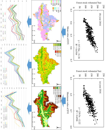
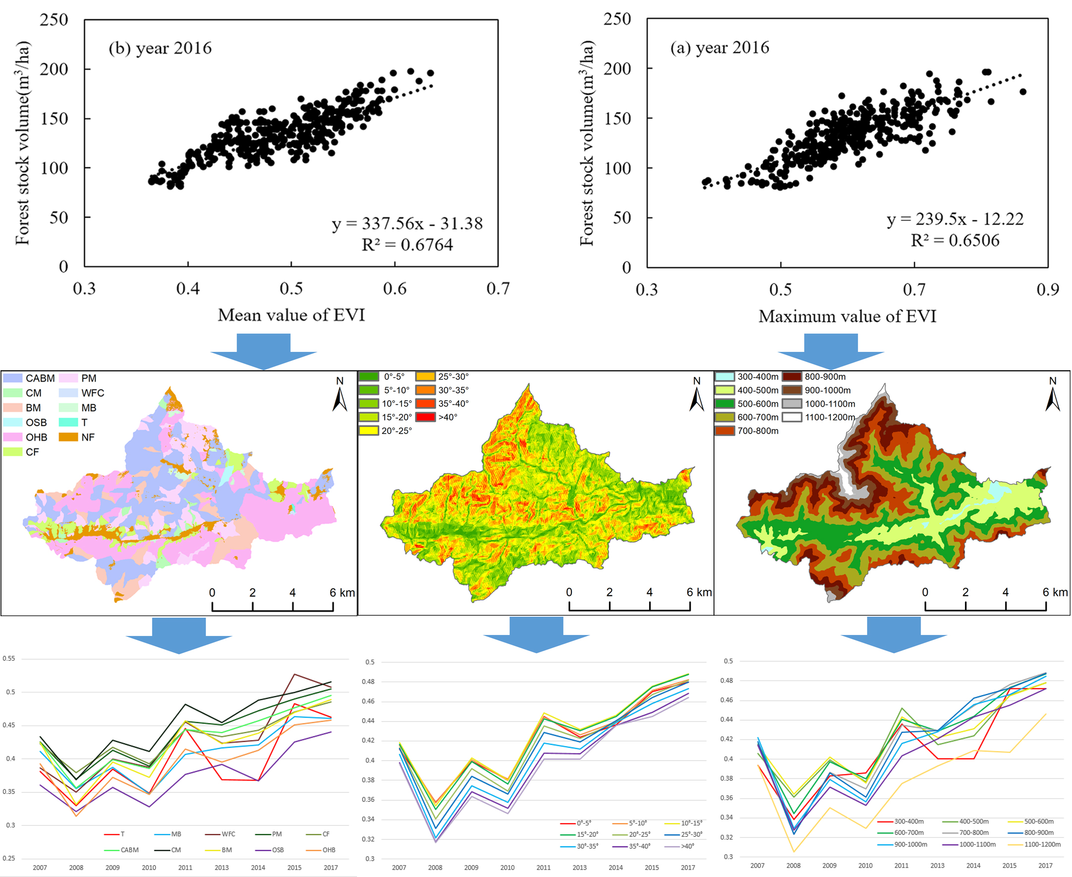
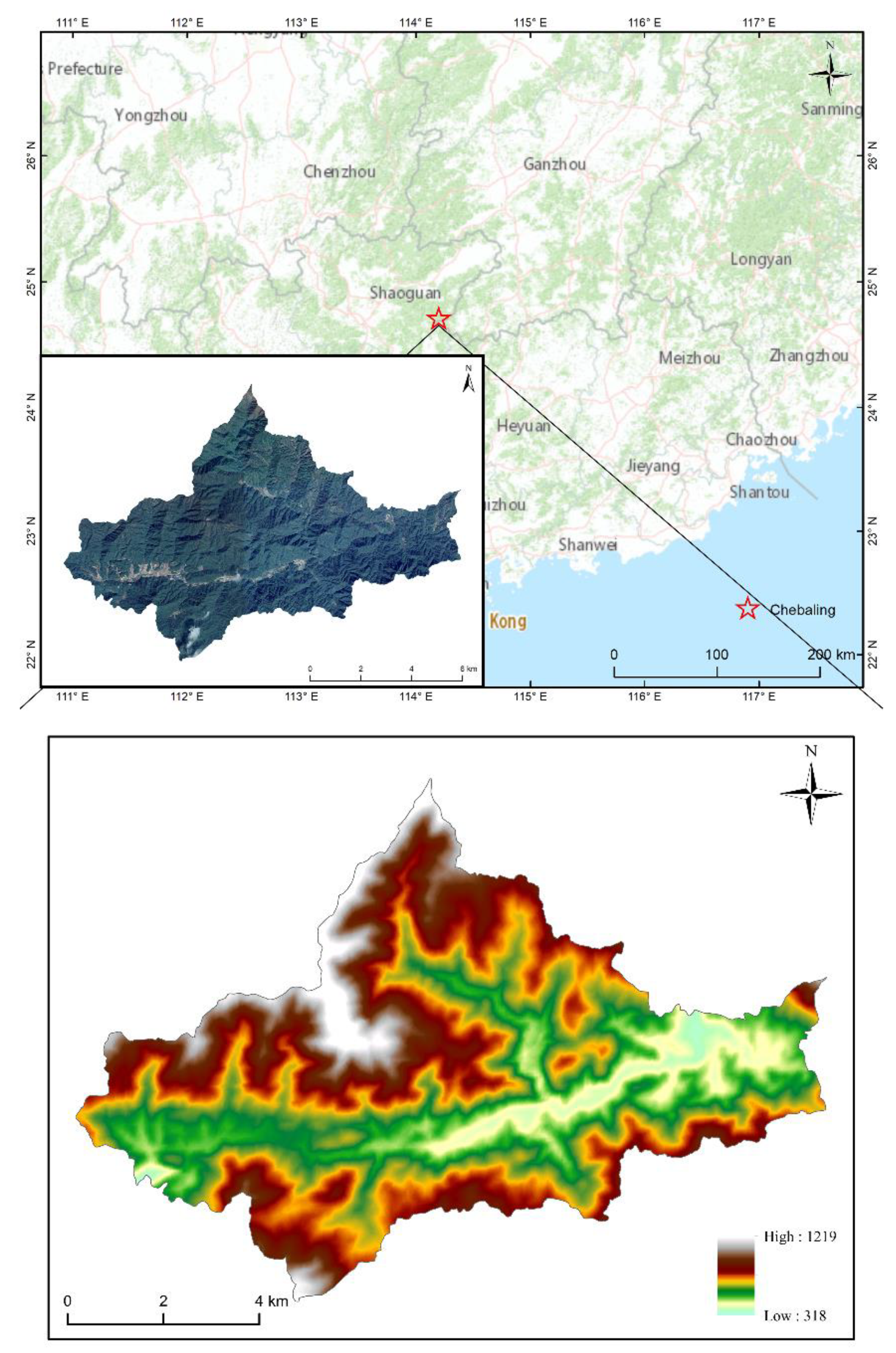
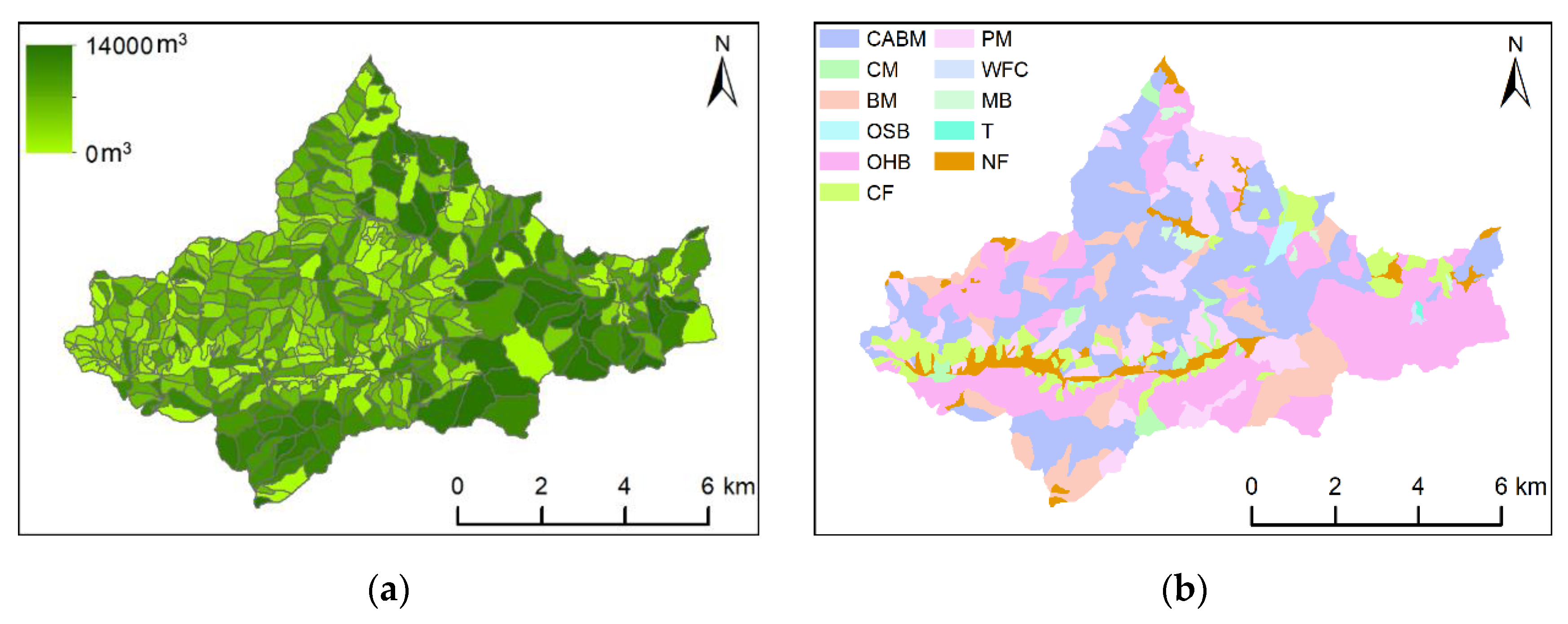
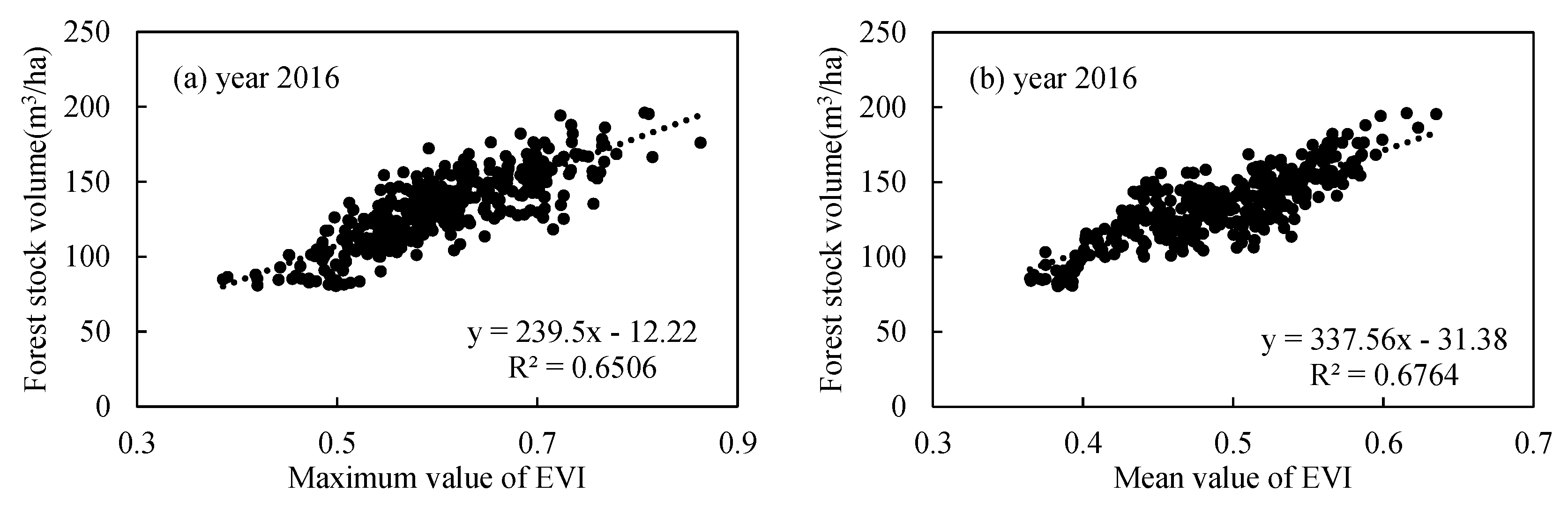
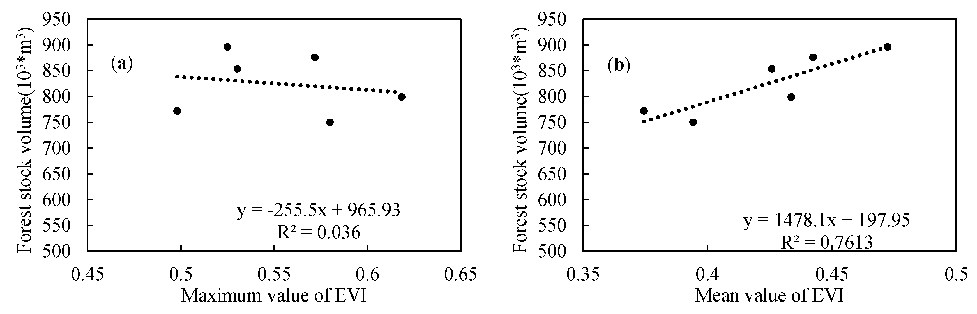
In this study, we sought to evaluate the impact of the ice storm, as well as the naturally occurring post-disaster forest recovery. We focused on the Chebaling National Nature Reserve, an important area of protected subtropical forest in China which supports numerous rare wild animals and plants. Our main objective was to investigate spatial and temporal variations in forest damage and recovery after the ice storm. First of all, spatial correction between the forest stock volume given by the sub-compartment data and the remotely sensed EVI (Enhanced vegetation index) was carried out to verify the feasibility of replacing the forest stock volume with remotely sensed EVI data. Then, in terms of disaster impact and post-disaster recovery, we analyzed the impact of elevation, slope, and forest types on EVI change from 2007 to 2017. Finally, in this paper, we summarized the characteristics of the impact of the disaster on the forest in Chebaling, as well as the characteristics of the post-disaster recovery, and preliminarily discussed the causes of the phenomenon. This study has important implications for the evaluation of disaster impacts and for medium-scale studies of long-term natural recovery processes following natural disasters.

2. Materials and Methods

2.1. Study Area

Our study area was located in the Chebaling National Nature Reserve (24°40′–24°46′N, 114°07′–114°16′E), Guangdong Province, China (Figure 1). Chebaling is considered important for protecting typical subtropical evergreen broadleaf forests and rare flora and fauna [28,29]. It was established in 1981 and upgraded to a national nature reserve in 1989. Chebaling encompasses an area of 7545 ha, and there are 1928 plant species and 1558 animal species present within the reserve [28]. The climate of Chebaling is classed as moist, moderate subtropical monsoon; the topography in the region is complex, with an elevation range of 318–1219 m above sea level. The landform is characterized by mountainous areas that are typical of the South China fold system. The average annual temperature is 19.6 °C, and annual precipitation is 1467 mm. Chebaling is located in the transition zone from the southern subtropical area to the middle subtropical area and is dominated by primary evergreen broad-leaved forest. Planted forest, cultivated land, and villages are limited to the flat central area. The ice storm in 2008 had a serious impact on the forest in Chebaling. In the past ten years, the forest has gradually been restored, and the natural forest has been largely unaffected by human disturbance during the restoration period. The modest area and complex topography of Chebaling enable us to analyze the characteristics of natural forest recovery and how these vary according to the vertical zone.

2.2. Data

2.2.1. Remote-Sensing Data

The most important remote-sensing parameter used in this study was the Enhanced Vegetation Index (EVI). Vegetation indices are often used to assess vegetation status and forest recovery. In the various vegetation indices, the EVI and Normalized Difference Vegetation Index (NDVI) are the most commonly used in forest ecology studies. The study area was located in the subtropical zone, so, in order to avoid saturation of the vegetation index in this area of lush vegetation [30], we chose the EVI as the main vegetation index to be used. The EVI is a common vegetation index that was developed to improve sensitivity in high biomass regions and to improve vegetation monitoring through a de-coupling of the canopy background signal and atmospheric influences [31,32]. In this study, we took one calendar year as the basic time unit, and annual composites of the EVI data were made. We intended to focus on the average and best state of the forest for each year, and so we calculated the annual mean EVI and annual maximum EVI for the forest in Chebaling. Annual EVI data were derived from Landsat TM, ETM+, and OLI composites (path 122, row 43; UTM zone 49 N). We obtained data by using the Climate Engine (https://clim-engine.appspot.com/). These remote-sensing data have been processed in the Climate Engine, including radiometrically and atmospherically corrected. Then, the annual EVI data were made by using all the available cloud-free Landsat data for the selected calendar years. The years from 2007 to 2011 relied on Landsat 5 TM data, whereas 2012 relied on Landsat 7 ETM+ data; more recent observations used Landsat 8 OLI data. A few pixels (<2% each year) were of poor quality and were excluded from the analysis.

In addition, digital elevation model (DEM) data, GF-1 satellite data, and 9 cloud-free Landsat scenes acquired at specific times were also used in this study. DEM data were used to extract elevation and slope factors, while GF-1 and cloud-free Landsat images were used for classification. The DEM data were derived from ASTER GDEM data provided by NASA and had a spatial resolution of 30 m. The GF-1 multispectral satellite images had a resolution of 2 m and were acquired on 15 February 2017. The cloud-free Landsat data were acquired from the United States Geological Survey (https://espa.cr.usgs.gov) and the Landsat satellite program [33,34]. The data acquisition times were concentrated in the dry season, i.e., from October to December of each year, from 2008 to 2017, with the exception of 2010 (26 March), 2011 (20 August), and 2012 (no data). Further information about the cloud-free Landsat data is shown in

Table 1. Cloud-free Landsat data details.

Year	Satellite	Data Acquisition Time
2008	Landsat-5	17 December 2008
2009	Landsat-5	4 December 2009
2010	Landsat-5	26 March 2010
2011	Landsat-5	20 August 2011
2013	Landsat-8	29 November 2013
2014	Landsat-8	18 December 2014
2015	Landsat-8	18 October 2015
2016	Landsat-8	7 December 2016
2017	Landsat-8	26 December 2017

.

2.2.2. Forestry Sub-Compartment Data

The sub-compartment is the basic unit of forest resource statistics and management. The forestry and biological characteristics of forests in the same sub-compartment are basically the same. After the 2008 ice storm, the management department of Chebaling conducted annual field surveys of the forest in the reserve, using forestry sub-compartments as the basic unit. We acquired these data (covering 2009 to 2016) and used them to verify and supplement the satellite data. Chebaling is divided into 451 sub-compartments, among which 423 sub-compartments are covered by different tree species. The forest stock volume and main forest types in each sub-compartment were the main parameters used in this study: these are the most important factors for the investigation of forest stands [35] and the main indicators used to evaluate forests. Figure 2a shows the spatial distribution of forest stock volume for 2016. Forest stock volume is one of the best predictors of biomass at the stand level [36]. Moreover, as an important tool in the understanding of forest dynamics, it can be used to predict whether a forest will act as a CO₂ emission source or sink [37]. Therefore, the state of regional forests can be reliably described by using the forest stock volume, and the forest stock volume can also be used as the ground verification data for remote-sensing parameters. In the sub-compartment data, the forest in Chebaling was divided into 10 main types (Figure 2b): tea (T), moso bamboo (MB), woody fruit crops (WFC), Pinus massoniana (PM), Chinese fir (CF), coniferous and broad-leaved mixed forest (CABM), coniferous mixed forest (CM), broad-leaved mixed forest (BM), other softwood broadleaved forests (OSB), and other hardwood broadleaved forests (OHB). In addition, there was a NF (non-forest) class. The forest sub-compartment data thus included a large number of forest types and were highly accurate; the data were used to supplement the remote-sensing data in the research.

2.3. Method

In this section, data analysis and data-processing methods were used to verify the feasibility of replacing the actual state of forest with the remote-sensing vegetation index and to extract 3 important factors (forest types, elevation zones, and slope zones) from multisource data for subsequent study.

2.3.1. Correlation Analysis

By studying the correlation between various remote-sensing vegetation indices and measured forestry data, scholars have evaluated the feasibility of using remote-sensing data to study forest changes, as well as the applicability of various remote-sensing indices [38,39,40]. Macedo et al. [41] used forest inventory data (24 plots) and forest indices (NDVI, EVI, SR, and SAVI) derived from high-spatial-resolution satellite images, to estimate and map the aboveground biomass of Mediterranean Quercus rotundifolia in Southern Portugal. Correlation analysis, variance analysis, and linear regression were used in their study; the simple ratio (SR) median value was considered to be the best predictor (R² = 75.3) of the aboveground biomass. Bolton et al. [42] used samples of ALS data and Landsat time-series metrics to produce estimates of the top height, basal area, and net stem volume for two timber-supply areas near Kamloops, British Columbia, Canada, using an imputation approach. Their results showed that Landsat-imputed attributes correlated strongly with ALS-based estimates in these blocks (R² = 0.62 and relative RMSE = 13.1% for top height, R² = 0.75 and relative RMSE = 17.8% for basal area, and R² = 0.67 and relative RMSE = 26.5% for net stem volume) and that remote sensing data could be used to produce wall-to-wall estimates of key inventory attributes. On the basis of the results of previous studies, we analyzed the correlation between EVI (annual mean EVI and annual maximum EVI) and forest stock volume in Chebaling in terms of both spatial correlation and temporal correlation.

A linear regression analysis was conducted to identify the relationship between the forest stock volume at the sub-compartment scale and the maximum and mean values of EVI within each sub-compartment. The linear regression model used was as follows:

SV = a1 + a2·EVI

(1)

where SV is the forest stock volume, EVI is the maximum or mean value of the EVI within each sub-compartment, and a1 and a2 are regression coefficients.

• Spatial Correlation

Figure 3a,b respectively show the relationship between the forest stock volume and the maximum value of the EVI and the mean value of the EVI at the sub-compartment scale in 2016. R², which represents the goodness of the fit between the maximum EVI value and the forest stock volume, varies from 0.62 to 0.71. The mean value of R² for these 8 years is 0.6721. R² for the correlation between the mean value of the EVI and the forest stock volume varies from 0.63 to 0.70, with a mean value of 0.6737. These significant correlations indicate that the spatial relationship between the forest stock volume and the mean value of the EVI is similar to that between the stock volume and the maximum value of the EVI.

2.

Temporal Correlation

The mean and maximum values of the EVI in Chebaling for the years 2009–2016, combined with the forest stock volume for each year, were used to analyze the temporal correlation between the variables. Because of the low quality of the Landsat-7 data from 2012 and the fluctuations in EVI caused by there being insufficient data after cloud removal in 2016, the correlation was recalculated after removing these two years (Figure 4). R² between the mean value of the EVI and the forest stock volume is 0.7613, indicating a strong correlation between them. However, there is no correlation between the maximum value of the EVI and the forest stock volume (R² = 0.036).

Based on the above correlation analysis results, it can be seen that the mean EVI value has a strong correlation with the forest stock volume, both temporally and spatially, and can, therefore, be used to represent the forest stock volume. The mean value of the EVI was thus used for subsequent disaster impact and post-disaster recovery analysis.

2.3.2. Classification

The classification of forest types based on remote-sensing data is the key and also the most difficult point in the application of remote-sensing technology to forestry. At present, there are many studies on identifying vegetation and forest types by using medium- and low-resolution remote-sensing data [43,44,45]; in contrast, there is a lack of forest-type classification based on high-resolution remote-sensing data [46,47], and related theories and methods are still at the initial stage because of unsatisfactory classification results. However, remote-sensing classification is able to distinguish between forest and non-forest (NF) categories well.

Information about the main forest types in each sub-compartment can be obtained through field surveys, which are more accurate and detailed than that obtained via the remote-sensing method. However, the accuracy of forest boundary information derived from forestry sub-compartment data is poor, and the update frequency cannot meet practical and research needs. By comprehensively utilizing remote-sensing classification results and sub-compartment forest types information, it is possible to refine the boundaries of different forest types; this is beneficial to studies of the difference in recovery between different forest types after ice storm.

Using remote sensing image process software ENVI5.3, we preprocessed (atmospherically and radiometrically corrected) 9 cloud-free Landsat scenes—one from each year from 2008 to 2017 with the exception of 2012—and used the maximum likelihood classification method [48] to classify the processed data. As these are medium-resolution remote-sensing data, only four classification categories were used: forest, water, cultivated land and buildings, and bare land. The proportions of each category are shown in

Table 2. Landsat land-use classification results (2008–2017).

Year	Bare Land	Cultivated Land and Buildings	Water	Forest
2008	0.68%	1.84%	0%	97.48%
2009	0.68%	1.89%	0%	97.43%
2010	0.70%	2.01%	0.03%	97.26%
2011	0.58%	2.11%	0.03%	97.28%
2013	0.55%	2.07%	0.03%	97.35%
2014	0.46%	2.06%	0.03%	97.45%
2015	0.52%	2.13%	0.03%	97.32%
2016	0.81%	2.04%	0.03%	97.12%
2017	0.61%	2.18%	0.03%	97.18%

. According to the classification results, the distribution and proportion of land-use types in Chebaling varied little from 2009 to 2017. Therefore, it was possible to use the 2017 forest boundary to represent the Chebaling forest boundary for the ten-year period studied.

The image used for the 2017 classification was acquired by the GF-1 remote-sensing satellite. Geometric registration, radiometric correction, orthophoto correction, and band fusion were carried out by ENVI5.3, to obtain the standard image. The classification method we used was the object-based random forest method, which is one of the most accurate and widely used algorithms [49,50,51,52,53] for remote-sensing image classification. The classification software used was eCognition, a professional remote-sensing image-classification software. Based on the results of several experiments, the final classification parameter settings were determined. The parameters for the segmentation process were (1) scale parameter: 50; (2) composition of homogeneity criterion: shape: 0.2, compactness: 0.5. The parameters for the classification characteristics included spectral characteristics (mean value and standard deviation of each band, NDVI), geometric characteristics (border index, shape index), and texture characteristics (GLCM Entropy, GLCM Mean, GLCM Standard Deviation, and GLCM Correlation), giving a total of 15 parameters. The overall accuracy of the classification results obtained was 96.5478%, and the kappa coefficient was 0.9544. The classification map is shown in Figure 5a. Based on the classification results, and in combination with the forest types and boundary information derived from the forestry sub-compartment data, the final forest-types distribution map for Chebaling was generated (Figure 5b), and the areas of different forest types were shown in

Table 3. Areas of different forest types in Chebaling.

Forest Types	T	MB	WFC	PM	CF	CABM	CM	BM	OSB	OHB
Area (ha)	5	61	5	892	445	2386	131	770	39	2243

.

2.3.3. Grading Methods for Elevation and Slope

Based on the DEM data and actual situation of terrain, Chebaling was divided into 9 elevation zones with 100 m intervals and 9 slope zones with 5-degree intervals. The forest area and percentage coverage in each elevation and slope zone are shown in

Table 4. Details of the elevation and slope zones.

Elevation (m)	Forest Area (ha)	Land Area (ha)	Forest Proportion	Slope (°)	Forest Area (ha)	Land Area (ha)	Forest Proportion
300–400	93	116	79.99%	0–5	173	242	71.60%
400–500	993	1133	87.62%	5–10	686	788	87.04%
500–600	1654	1771	93.37%	10–15	1268	1346	94.24%
600–700	1711	1728	99.03%	15–20	1609	1658	97.05%
700–800	1317	1338	98.36%	20–25	1546	1581	97.80%
800–900	716	731	97.89%	25–30	1133	1159	97.81%
900–1000	414	432	95.74%	30–35	553	569	97.11%
1000–1100	223	240	92.91%	35–40	167	172	97.03%
1100–1200	58	68	84.46%	>40	44	46	95.49%

. However, only changes in the forest were considered in this study, so the non-forest area was not included in the subsequent analysis. Figure 6 shows the spatial distribution of the elevation and slope zones.

3. Results

In the previous section, the feasibility of using the annual mean value of the EVI (referred to simply as the EVI from now on) to represent the forest stock volume was demonstrated. Therefore, the EVI was used to represent the status of the forest for the study of disaster impact and post-disaster recovery from 2007 to 2017. EVI of 2012 and 2016 were not used in our study, and the reasons were discussed in the analysis in Section 2.3.1. Therefore, we used the EVI of the remaining nine years of the period 2007–2017 for disaster study. In this section, the difference of disaster impact and post-disaster recovery in different elevation zones, slope zones, and for different forest types are analyzed from two aspects of single factor and multiple factor respectively.

3.1. Single-Factor Analysis

3.1.1. Disaster Analysis in Different Elevation Zones

The broken-line graph (Figure 7) shows the change in EVI in different elevation zones from 2007 to 2017. First, in terms of the impact of disasters, the EVI of forests in all elevation zones were greatly reduced due to the ice storm from 2007–2008. However, the EVI decreased more in middle- and high-elevation zones (green, blue, and purple) than in low-elevation zones (red, orange, and yellow). Second, in terms of post-disaster recovery, although in some years (2008–2011) the EVI fluctuated slightly, the overall trend was that there was a rise in EVI in all zones, meaning that the lowest value occurred in 2008 and the highest value in 2017. From 2008 to 2011, the EVI in the 400–600 m zones was the highest in Chebaling. However, after 2013, the EVI in the higher altitude areas, particularly in 600–1000 m zones, gradually exceeded that in the 400–600 m zones. During this period, there was a continuous gentle rise in EVI at elevations above 600 m. In contrast, below 600 m, the EVI fluctuated greatly.

Table 5. Details of the disaster impact and post-disaster recovery in different elevation zones. In the property row of the table, disaster impact refers to the absolute value of EVI difference between 2008 and 2007; post-disaster recovery refers to the absolute value of EVI difference between 2017 and 2008; fluctuation degree represents the fluctuation of EVI from 2008 to 2017; H, M, and L in fluctuation-degree column represent high, medium, and low, respectively.

Elevation (m)	EVI (2007)	EVI (2008)	EVI (2017)	Disaster Impact	Post-Disaster Recovery	Fluctuation Degree
300–400	0.394	0.338	0.472	0.055	0.134	H
400–500	0.406	0.361	0.478	0.045	0.117	H
500–600	0.414	0.364	0.478	0.050	0.114	H
600–700	0.416	0.344	0.487	0.071	0.143	M
700–800	0.415	0.324	0.488	0.091	0.165	M
800–900	0.418	0.324	0.488	0.094	0.164	M
900–1000	0.422	0.329	0.485	0.093	0.156	L
1000–1100	0.414	0.327	0.472	0.087	0.144	L
1100–1200	0.394	0.306	0.446	0.088	0.141	L

gives the results of a comprehensive analysis of the disaster impact and the recovery after the disaster. The first thing to explain here is the calculation method of fluctuation degree in Table 5 and following several tables, taking the fluctuation degree of elevation zones in Table 5 as an example. First, the standard deviation of annual EVI growth value from 2008 to 2017 in each elevation zone was calculated. Second, the initial classification of fluctuation degree was calculated. If there was no significant difference between the standard deviation of EVI growth value in each elevation zone, the fluctuation degree of all elevation zones would be set as L. If there was a significant difference between the standard deviation in each elevation zone, the two or three highest values would be set as H, the two or three lowest values would be set as L, and the others would be set as M. Third, the final classification of fluctuation degree was calculated. According to the broken-line graph of EVI changes from 2007 to 2017 in different elevation zones, if the EVI change trend of one elevation zone was different from that of most other elevation zones, or the fluctuation amplitude of several years were significantly higher than that of other elevation zones, the fluctuation degree of this elevation zone would increase by one level (L increases to M, M increases to H, H remains unchanged). Otherwise, the fluctuation degree would remain unchanged.

As shown in Table 5, the forest in the 700–1000 m elevation zones (the three red rows) had a high EVI value before the disaster. Although the impact of the disaster was relatively severe in these zones, the post-disaster recovery rate and increase value of EVI were also the highest, and the recovery process was quite smooth and without any big fluctuations. Conversely, the EVI in the 300–600 m elevation zones (the three blue rows) was relatively low before the disaster and decreased little after the disaster; however, the recovery rate was slow and the EVI fluctuated greatly. This indicates that the forest in the high-altitude area of Chebaling was seriously affected by the disaster but also showed a stronger post-disaster recovery ability.

3.1.2. Disaster Analysis in Different Slope Zones

The change trend of the EVI in each slope zone from 2007 to 2017 is shown in Figure 8. From 2007 to 2008, EVI in all slope zones decreased significantly, and the decrease value in high slope zones were slightly higher than that in low slope zones. From 2008 to 2017, the change trends in EVI in different slope zones are similar. Before 2011, the EVI increased or decreased by about the same amount in each slope zone every year, and so the differences between the absolute values of the EVI remained constant. However, the differences between the absolute values of the EVI in different slope zones decreased significantly after 2011, especially from 2013 to 2015, as the degree of recovery in the different slope zones started to vary. Overall, the forest recovery in the areas with steeper slopes was better than that in the less-steep areas between 2008 and 2017.

The results of the analysis of the disaster impact and disaster recovery for all of the slope zones are summarized in

Table 6. Details of the disaster impact and post-disaster recovery in different slope zones.

Slope (°)	EVI (2007)	EVI (2008)	EVI (2017)	Disaster Impact	Post-Disaster Recovery	Fluctuation Degree
0–5	0.412	0.357	0.480	0.055	0.122	L
5–10	0.415	0.357	0.482	0.058	0.125	L
10–15	0.419	0.354	0.488	0.064	0.134	L
15–20	0.416	0.351	0.488	0.066	0.137	L
20–25	0.413	0.341	0.482	0.072	0.141	L
25–30	0.412	0.331	0.480	0.081	0.148	L
30–35	0.406	0.322	0.473	0.084	0.152	L
35–40	0.398	0.317	0.469	0.081	0.152	L
>40	0.397	0.317	0.464	0.080	0.148	L

. Before the ice storm, the EVI values in the zones with slopes between 5° and 25° were the highest. However, the impact of the disaster on the forest in Chebaling increased gradually as the slope increased. As a result, in 2008, areas of forest on steeper slopes had lower EVI values. During the post-disaster recovery process from 2008 to 2017, the change trends in EVI in all of the slope zones were basically the same, and the amount of fluctuation was small. There was a positive correlation between the degree of disaster recovery and the degree of disaster impact. Therefore, the ranking of slopes zones by EVI value in 2017 was same as that in 2007.

3.1.3. Disaster Analysis for Different Forest Types

Figure 9 shows the trends in EVI for different forest types from 2007 to 2018. Following the disaster, EVI for BM and OHB decreased the most; however, EVI for WFC decreased the least. In terms of post-disaster recovery, the EVI trends for the planted forest types (T and WFC) were significantly different from those for the other eight forest types. The T and WFC EVI values fluctuated a lot, with the EVI for T always being lower than that for WFC. The EVI for T and WFC reached the peak in 2015, showing that the planted forest can recover to a high EVI level faster. The EVI trends for PM, CABM, and CF were basically the same, with the EVI rising steadily and showing little fluctuation. Moreover, the EVI for these three forest types were higher than those for the other types (except CM and BM) most of the time. The EVI trends for CM and BM were similar and CM had the highest EVI value in most years. Although the EVI for BM was lower than EVI for the CM, CF, PM, and CABM in 2008, it increased rapidly after that and was one of the highest values in 2017. In contrast, the EVI for CM and BM fluctuated slightly more than for the CF, PM, and CABM. The MB EVI was moderately high in 2008, but its growth rate was low from 2008 to 2017, which lead to this value being low in 2017. The EVI for OHB was low in 2008 and changed in a similar way to the BM and CM; however, it was always 0.02 to 0.03 lower than the BM EVI. The EVI for OSB did not rise as quickly as the EVI for the other forest types. This EVI was the lowest in most years; in addition, its value fluctuated more than all the other EVI values, except those for the two planted forest types (T and WFC).

The results of the analysis of the disaster impact and post-disaster recovery for the different forest types are shown in

Table 7. Details of the disaster impact and post-disaster recovery for different forest types.

Forest Types	EVI (2007)	EVI (2008)	EVI (2017)	Disaster Impact	Post-Disaster Recovery	Fluctuation Degree
T	0.381	0.329	0.462	0.052	0.133	H
MB	0.411	0.356	0.460	0.055	0.105	M
WFC	0.386	0.350	0.508	0.036	0.158	H
PM	0.426	0.370	0.505	0.056	0.135	L
CF	0.423	0.379	0.486	0.043	0.107	L
CABM	0.425	0.356	0.496	0.068	0.139	L
CM	0.433	0.369	0.515	0.065	0.147	M
BM	0.424	0.331	0.489	0.093	0.158	M
OSB	0.361	0.321	0.440	0.040	0.119	M
OHB	0.392	0.314	0.458	0.078	0.144	M

. The damage caused by the disaster was less in the areas covered by planted forest (T and WFC) than in the areas of natural forest. In addition, the EVI for the planted forest areas fluctuated greatly during the post-disaster recovery process. Before the disaster, the EVI for the coniferous forest (CF, PM, and CM areas) and CABM were higher than for most of the other forest types. These four forest types were less affected by the disaster than the broad-leaved forest, and the EVI in these areas showed a relatively steady rise during the post-disaster recovery. BM and OHB were seriously affected by the disaster but recovered quickly—the EVI here fluctuated slightly more than for the coniferous forests. OSB had a low degree of disaster impact and post-disaster recovery, which can be attributed to its low EVI value before the disaster. MB was moderately affected by the disaster, and its EVI value increased the least after the disaster.

3.2. Multifactor Comprehensive Analysis

We have analyzed the relationship between EVI change and single factor (elevation, slope, and forest type) from 2007 to 2017. However, the spatial distribution of 10 forest types were different from each other; for example, the forest-types distributed in the 400–500 m zone were different from those in the 900–1000 m zone, and WFC and PM grew in regions with different elevation and slope. Therefore, disaster analysis for different forest types needs to be further studied. Multifactor analysis was carried out for this section. We combined forest types with elevation zones and slope zones, respectively, for a comprehensive analysis and used control variable method to improve the accuracy of analysis results.

We calculated the distribution proportion for 10 forest types in different elevation and slope zones and found that the numbers for forest types distributed in the four elevation zones (400–800 m) and four slope zones (10–30°) were bigger than in other elevation and slope zones. Moreover, the area of these elevation and slope zones was larger than that of other elevation and slope zones (Table 4). Therefore, we selected these elevation and slope zones for multifactor analysis. Similarly, the areas for six forest types (PM, CF, CM, CABM, BM, and OHB) were larger than other forest types (Table 3), and these six forest types had wider ranges of elevations and slopes. As a result, these six forest types were selected for multifactor analysis.

3.2.1. Disaster Analysis for Different Forest Types in Four Elevation Zones

According to the EVI trend for different forest types in the four elevation zones (Figure 10), combined with the statistical table of disaster analysis (

Table 8. Disaster-impact-analysis results for different forest types in four elevation zones.

Forest Types	Disaster Impact				Average Value of Disaster-Impact Ranking
	400 m–500 m	500 m–600 m	600 m–700 m	700 m–800 m
T	0.052	-	-	-	-
MB	0.041	0.060	0.045	0.068	5
WFC	0.036	-	-	-	-
PM	0.030	0.038	0.048	0.068	6.25
CF	0.042	0.034	0.061	0.069	5
CABM	0.031	0.042	0.066	0.084	4.75
CM	0.020	0.029	0.076	0.099	5.75
BM	0.038	0.068	0.099	0.115	2
OSB	0.003	0.037	0.045	0.048	7.75
OHB	0.056	0.065	0.080	0.106	1.75

and

Table 9. Post-disaster recovery and fluctuation degree analysis results for different forest types in four elevation zones.

Forest Types	Post-Disaster Recovery/Fluctuation Degree				Average Value of Post-Disaster Recovery Ranking
	400 m–500 m	500 m–600 m	600 m–700 m	700 m–800 m
T	0.132/H	-	-	-	-
MB	0.066/M	0.060/M	0.045/M	0.068/H	5
WFC	0.161/H	-	-	-	-
PM	0.116/M	0.038/M	0.048/L	0.068/L	6.25
CF	0.119/L	0.034/L	0.061/M	0.069/M	5
CABM	0.109/L	0.042/L	0.066/L	0.084/L	4.75
CM	0.091/M	0.029/M	0.076/L	0.099/M	5.75
BM	0.126/M	0.068/H	0.099/H	0.115/H	2
OSB	0.082/M	0.037/M	0.045/M	0.048/M	7.75
OHB	0.122/L	0.065/H	0.080/H	0.106/M	1.75

), we comprehensively analyzed the relationship between EVI change and elevation for 10 forest types from three aspects: disaster impact, post-disaster recovery, and fluctuation degree in the recovery process. First, as shown in Figure 10 and Table 8, EVI for all forest types decreased more in higher elevation zones than in lower elevation zones from 2007 to 2008. EVI for OSB decreased the least, while EVI for BM and OHB decreased the most among all forest types. Second, the EVI change trend for most forest types from 2008 to 2017 fluctuated larger in the 400–500 m elevation zone than in other elevation zones above 500 m (Figure 10). Moreover, as the elevation increased, the values in the post-disaster recovery columns (Table 9) for most forest types increased, and the absolute value of EVI difference between coniferous forests (PM, CF, and CM) and broad-leaved forests (BM, OHB, and OSB) increased significantly. Third, T and WFC were only distributed in 400–500 m elevation zone. In the 400–500 m elevation zone, EVI for T decreased more than it did for the eight other forest types (except OSB), which indicated that T was highly affected by the disaster. In the post-disaster recovery process, the fluctuation degree and increased value of EVI for T and WFC were the highest among 10 forest types. Finally, among the eight forest types (not including WFC and T) distributed in the four elevation zones, the disaster impact and post-disaster recovery degree for BM and OHB were both higher than other forest types in the same elevation zone.

3.2.2. Disaster Analysis for Different Forest Types in Four Slope Zones

Statistics and an analysis were also conducted on four typical slope zones. Based on the information in Figure 11 and

Table 10. Disaster-impact-analysis results for different forest types in four slope zones.

Forest Types	Disaster Impact				Average Value of Disaster-Impact Ranking
	10–15°	15–20°	20–25°	25–30°
T	0.042	0.053	0.051	0.064	7.25
MB	0.057	0.057	0.060	0.049	5.25
WFC	0.043	0.030	0.052	-	8
PM	0.054	0.056	0.058	0.062	5.75
CF	0.038	0.046	0.052	0.067	7
CABM	0.066	0.062	0.065	0.076	3.25
CM	0.067	0.042	0.044	0.067	6.5
BM	0.091	0.094	0.096	0.097	1
OSB	0.046	0.048	0.049	0.038	8
OHB	0.073	0.073	0.079	0.087	2

and

Table 11. Post-disaster recovery and fluctuation-degree analysis results for different forest types in four slope zones.

Forest Types	Post-Disaster Recovery/Fluctuation Degree				Average Value of Post-Disaster Recovery Ranking
	10–15°	15–20°	20–25°	25–30°
T	0.146/H	0.133/H	0.141/H	0.127/H	4.75
MB	0.113/L	0.111/M	0.097/M	0.112/H	9.25
WFC	0.136/H	0.119/H	0.145/H	-	5
PM	0.132/M	0.138/L	0.134/L	0.141/M	5.75
CF	0.101/L	0.114/L	0.125/L	0.135/L	8.5
CABM	0.136/L	0.133/L	0.136/L	0.149/L	4.75
CM	0.147/M	0.119/M	0.130/M	0.142/M	5.25
BM	0.158/M	0.162/M	0.162/M	0.158/M	1
OSB	0.138/M	0.154/M	0.132/M	0.099/M	5.75
OHB	0.141/M	0.141/M	0.144/M	0.150/M	3

, we can draw the following conclusions. First, in the slope range of 10–30°, with the increase of slope, the disaster-impact degree for most forest types gradually increased. However, the increase of the disaster-impact degree caused by the rise of slope zones was obviously slighter than that caused by the rise of elevation zones. This indicates that elevation is more decisive than slope in disaster impact. Second, in the post-disaster recovery process, the fluctuation degree for each forest type was similar in different slope zones. However, the absolute value of EVI difference for different forest types gradually increased with the increase of slope. The EVI of coniferous forests (PM, CF, and CM) were significantly higher than that of broad-leaved forests (BM, OHB, and OSB) in high slope zones. Third, since T and WFC were only distributed in the 400–500 m elevation zone, compared with other forest types in the same slope zone, they were less affected by the disaster and had the highest fluctuation degree. Finally, in the comparison with different forest types in each slope zone, BM was most vulnerable to the disaster but also had the highest post-disaster recovery and fluctuation degree, followed by OHB.

3.2.3. Disaster Analysis for Six Forest Types

After disaster analysis in typical elevation and slope zones, we then analyzed the disaster impact and post-disaster recovery for six typical forest types. First, we studied the influence of elevation. In terms of disaster impact, according to the statistics in

Table 12. Disaster-impact-analysis results for six forest types in different elevation zones.

Elevation (m)	Disaster Impact
	BM	OHB	CABM	CM	CF	PM
300–400	0.048	0.061	0.038	-	0.054	0.021
400–500	0.039	0.056	0.032	0.020	0.042	0.030
500–600	0.070	0.065	0.042	0.029	0.034	0.038
600–700	0.100	0.081	0.066	0.076	0.061	0.048
700–800	0.115	0.106	0.084	0.097	0.075	0.069
800–900	0.112	0.106	0.085	0.060	-	0.088
900–1000	0.112	0.100	0.083	0.134	-	0.073
1000–1100	0.086	0.095	0.091	0.082	-	0.059
1100–1200	0.077	0.077	0.101	-	-	0.088

, the areas that were least affected by the disaster were distributed in lowest elevation zones for five forest types (not including CF); moreover, as the elevation increased, the degree of disaster impact gradually increased, or first rose and then fell. On the contrary, the degree of disaster impact first fell and then rose as the elevation increased for CF. The hardest-hit area of CABM and coniferous forests (CM and PM) were in higher elevation zones than that of broad-leaved forest (BM and OHB).

During the 10 years after the disaster, as shown in Figure 12, EVI for coniferous forests (PM, CM, and CF) in middle- and high-elevation zones were mostly higher than that in low-elevation zones. On the contrary, EVI for CABM and broad-leaved forests (BM and OHB) in middle- and low-elevation zones were higher than that in high-elevation zones. According to

Table 13. Post-disaster recovery and fluctuation degree analysis results for six forest types in different elevation zones.

Elevation (m)	Post-Disaster Recovery/Fluctuation Degree
	BM	OHB	CABM	CM	CF	PM
300–400	0.175/H	0.126/M	0.178/H	-	0.159/H	0.121/H
400–500	0.127/H	0.122/H	0.109/L	0.092/H	0.118/M	0.116/H
500–600	0.142/M	0.129/H	0.115/L	0.083/M	0.077/L	0.101/L
600–700	0.169/M	0.151/M	0.136/L	0.177/M	0.141/L	0.124/L
700–800	0.174/M	0.173/M	0.158/L	0.197/L	0.175/L	0.155/L
800–900	0.166/M	0.166/M	0.159/L	0.133/L	-	0.173/L
900–1000	0.153/L	0.165/L	0.148/L	0.223/M	-	0.166/L
1000–1100	0.145/L	0.141/L	0.147/L	0.190/H	-	0.157/M
1100–1200	0.134/L	0.125/L	0.146/L	-	-	0.141/M

, the highest value in post-disaster recovery columns for coniferous forests (PM and CM) were in higher elevation zones than for broad-leaved forests (BM and OHB), but they were all in the 600–1000 m elevation zones. The fluctuation degree for the six forest types in the low-elevation zones was the highest. However, the fluctuation degree for broad-leaved forests (BM and OHB) decreased gradually with the elevation increases, but the fluctuation degree for coniferous forests (PM and CM) in high-elevation zones was higher than in middle-elevation zones. Overall, CABM fluctuated little in all elevation zones, and its recovery process was relatively stable than the other five forest types.

In terms of slope study, we made a comprehensive analysis according to Figure 13 and

Table 14. Disaster-impact-analysis results for six forest types in different slope zones.

Slope (°)	Disaster Impact
	BM	OHB	CABM	CM	CF	PM
0–5	0.065	0.069	0.056	0.086	0.025	0.055
5–10	0.080	0.067	0.060	0.084	0.036	0.055
10–15	0.091	0.074	0.065	0.066	0.038	0.054
15–20	0.094	0.073	0.062	0.038	0.047	0.056
20–25	0.097	0.082	0.064	0.043	0.054	0.058
25–30	0.097	0.088	0.075	0.069	0.070	0.062
30–35	0.094	0.089	0.082	0.099	0.069	0.055
35–40	0.081	0.082	0.084	0.127	0.105	0.057
>40	0.062	0.070	0.090	0.118	0.088	0.052

and

Table 15. Post-disaster recovery and fluctuation-degree-analysis results for six forest types in different slope zones.

Slope (°)	Post-Disaster Recovery/Fluctuation Degree
	BM	OHB	CABM	CM	CF	PM
0–5	0.133/L	0.135/L	0.130/L	0.172/L	0.082/L	0.130/L
5–10	0.150/L	0.130/L	0.130/L	0.169/L	0.088/L	0.128/L
10–15	0.157/L	0.142/L	0.136/L	0.144/L	0.102/L	0.133/L
15–20	0.162/L	0.141/L	0.133/L	0.115/L	0.114/L	0.137/L
20–25	0.163/L	0.146/L	0.135/L	0.127/L	0.125/L	0.135/L
25–30	0.159/L	0.151/L	0.147/L	0.142/L	0.137/L	0.143/L
30–35	0.152/L	0.150/L	0.154/L	0.183/L	0.130/L	0.140/L
35–40	0.145/L	0.147/L	0.157/L	0.219/L	0.146/L	0.139/L
>40	0.131/L	0.134/L	0.159/L	0.204/L	0.164/L	0.121/L

, and compared it with the analysis of elevation. As shown in Figure 13, from 2007 to 2008, the decreased value of EVI in different slope zones showed a significant difference for CF and CM, but showed little difference for BM, OHB, PM, and CABM. Among six forest types (Table 14), as the increase of slope, the values in the disaster impact columns for CM showed a trend of first decrease and then increase, with the lowest value in 15–20° slope zone. These values for CF and CABM kept increasing as the slope increased. However, these values for the other three forest types (BM, OHB, and PM) showed a trend of first increase and then decrease as the slope increased. In general, the slope zones above 20° were the hardest-hit areas for all forest types. By comparing the difference of disaster-impact degree on different elevation and slope zones for six forest types, we can see that the influence of slope was greater than that of elevation on CF; the influence of elevation was greater than that of slope on PM, CABM, BM, and OHB; elevation and slope all had strong influence on CM.

In the post-disaster recovery process from 2008 to 2017, as shown in Figure 13, for three coniferous forests (PM, CF, and CM), EVI in middle- and high-slope zones were higher than that in low-slope zones; for two broad-leaved forests (BM and OHB), EVI in middle- and low-slope zones were always higher than that in high-slope zones. In addition, it can be seen from Table 14 and Table 15 that the increased value of EVI in the post-disaster recovery process for six forest types was positively correlated with the decreased value of EVI after the disaster. The slope zones that were seriously affected by the disaster also had higher recovery degree. Moreover, The EVI trend for six forest types were rising steadily in all slope zones, without any significant fluctuation.

4. Discussion

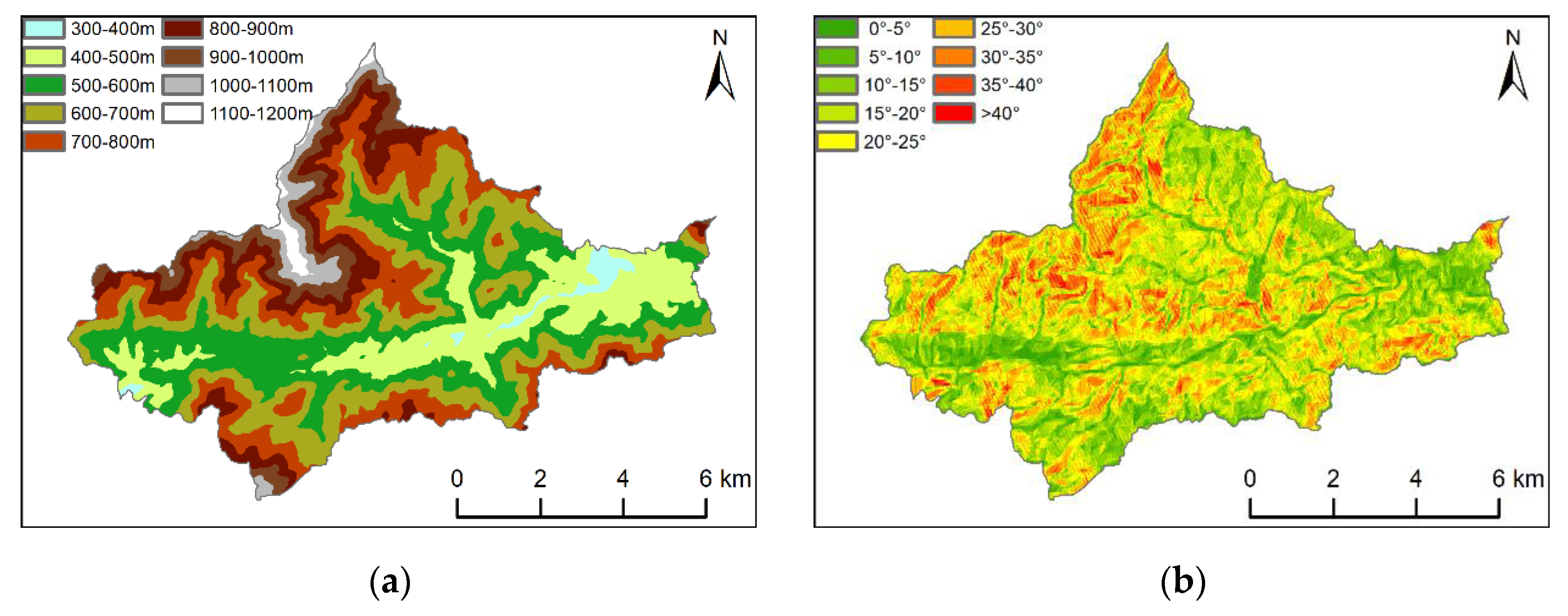
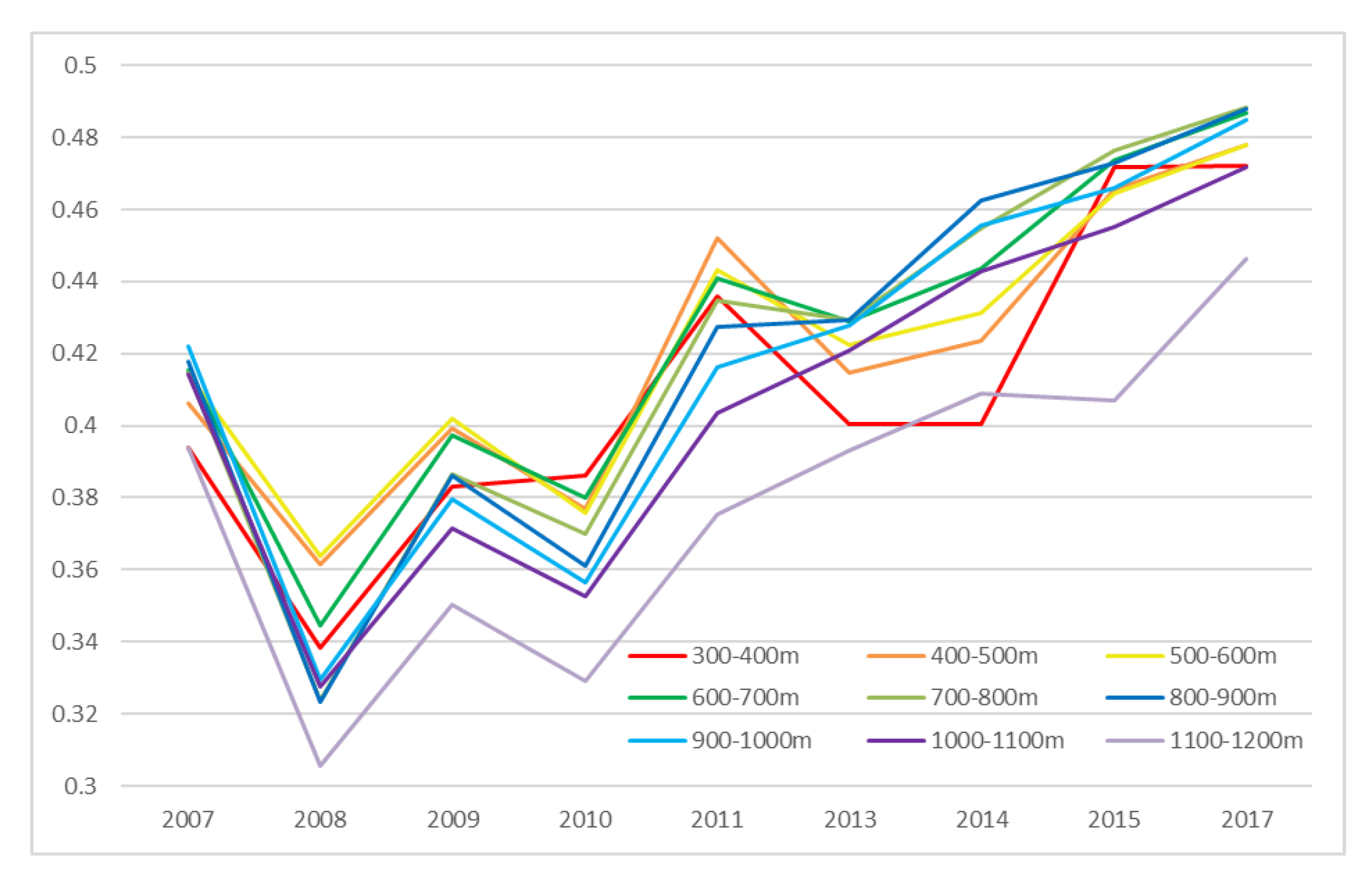
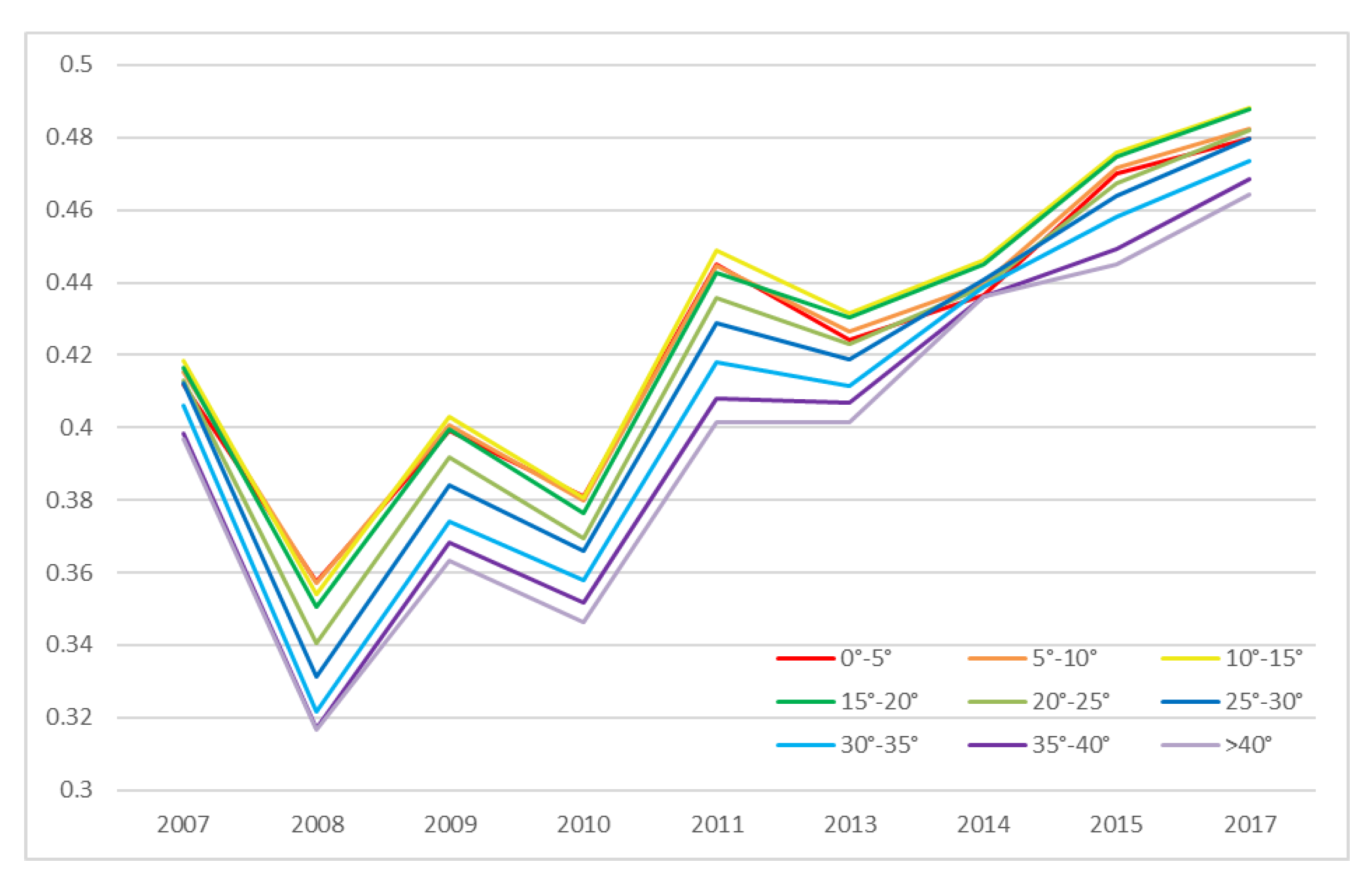
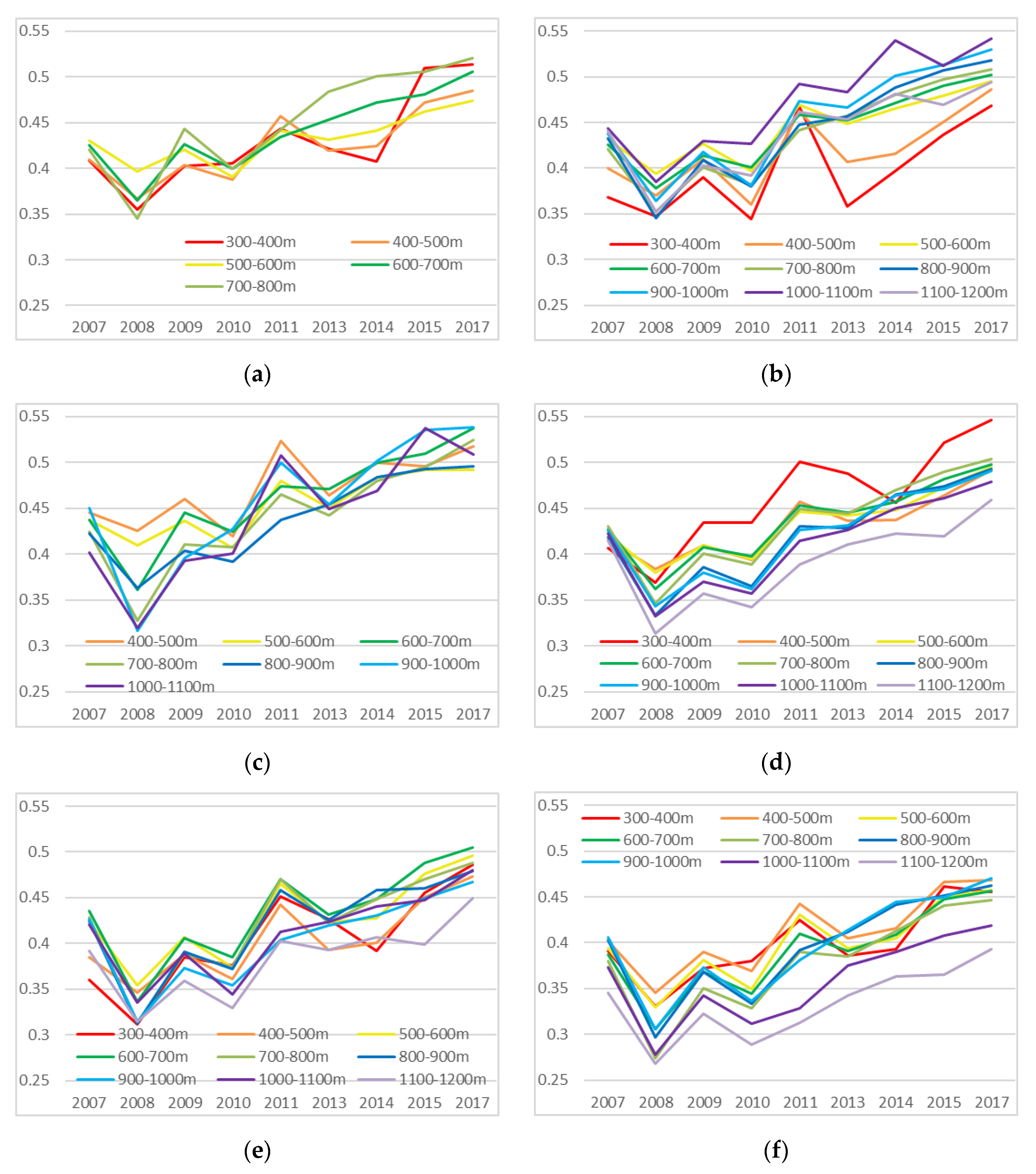
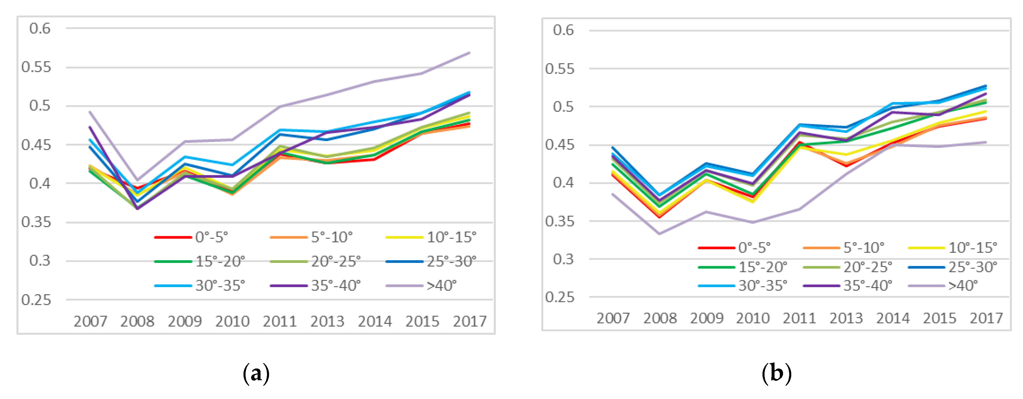
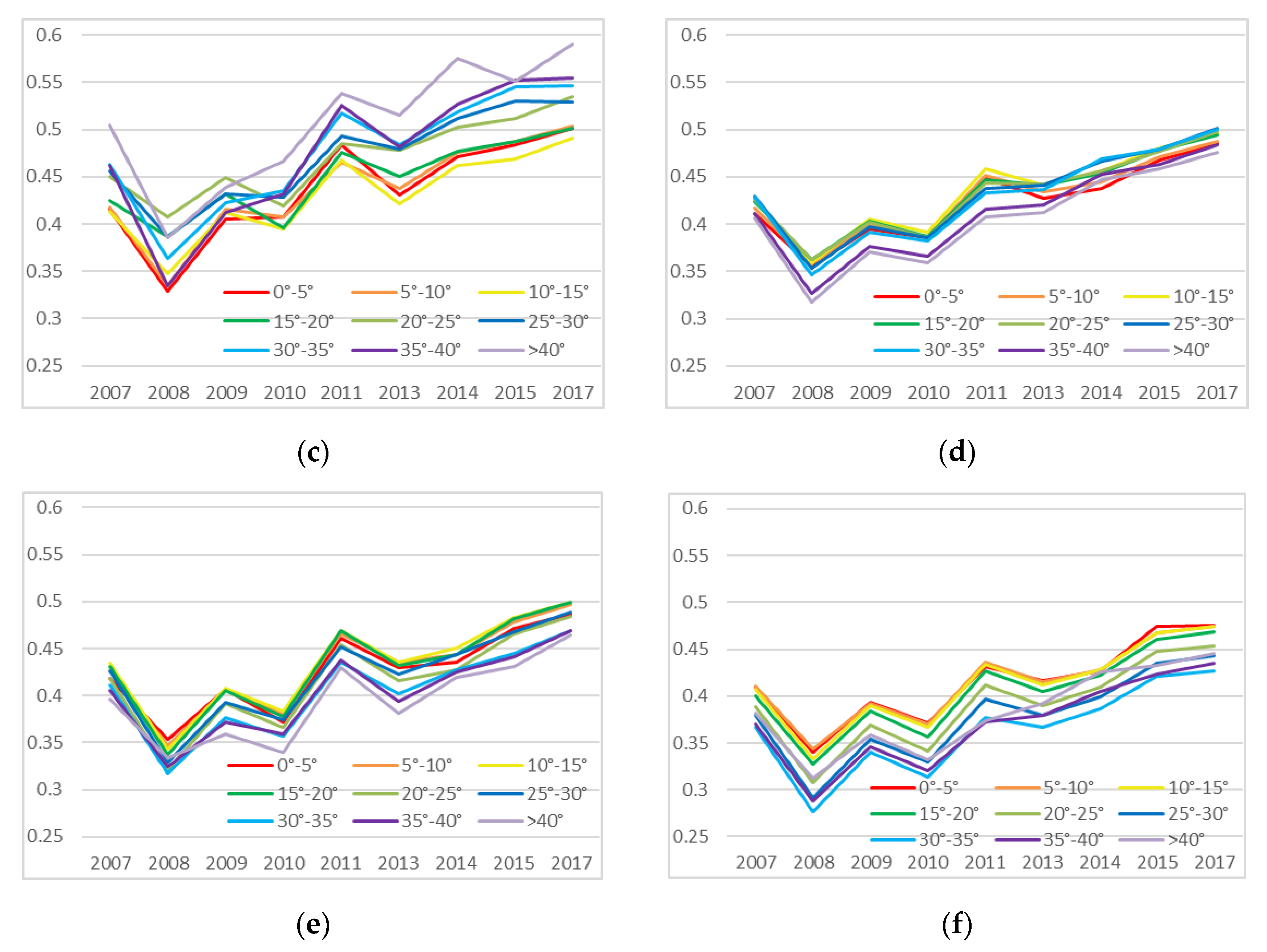
The results of quantitative analysis by remote sensing showed the difference of forest EVI change trend in a variety of topographic conditions after the ice storm. First, from the single-factor-analysis results, there were obvious differences in disaster impact and post-disaster recovery for different elevation and slope zones in the forest. Areas at an altitude of 700–1000 m and a slope of 25–40 degrees were most affected by the disaster but also had the highest post-disaster recovery degree. Next most affected were the highest-altitude areas above 1000 m and with the steepest slopes greater than 40 degrees. While the areas below 700 m and with slopes of 25 degrees or less were least affected by the disaster and had the lowest post-disaster recovery degree, but the fluctuation degree were high during the recovery process. Except for areas below 500 m, EVI for forest in other elevation and slope zones increased rapidly in the first three years (2009–2011) following the disaster, and the growth rate gradually slowed down in the later period. In addition, from the results of multifactor analysis, we find that the areas that were most affected by the disaster and had the highest recovery degree for coniferous forests had a higher altitude and steeper slope than broad-leaved forest.

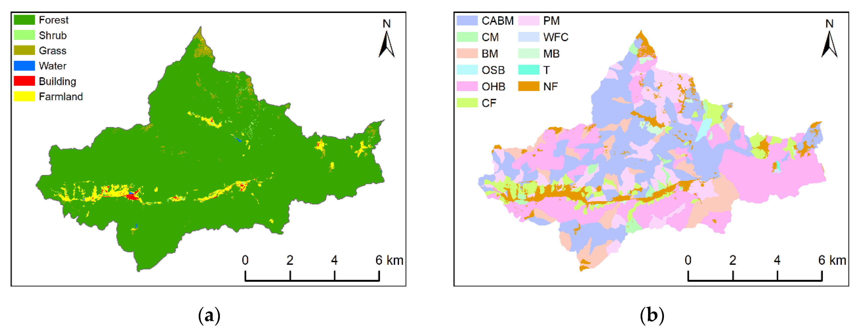
Based on the theoretical analysis and field investigation, we believe that the following were the most important factors behind this result. (1) Freezing rain, strong winds, and ice have a greater impact on regions at higher elevations and steeper slopes, which resulted in greater losses in these regions, as has similarly been demonstrated by other studies [6,54,55]. (2) Villages, farmland, and planted forests were distributed in the areas at a lower altitude and with a gentler slope. Therefore, these areas were greatly affected by human activities, leading to the highest level of EVI fluctuation during the disaster-recovery process. Areas with elevations of 700–1000 meters and slopes of 25–40 degrees were mainly covered by natural forest. The EVI in these areas was higher than in other areas before the disaster. Although these areas were seriously impacted by the disaster, and so the EVI here decreased more, the biological characteristics of natural forests enable them to recover quickly after disasters. Therefore, in the decade after the disaster, the EVI of the forest in this region increased the most. The forest density, average height, and diameter at breast height (DBH) are all affected by the topography, climate, and other factors, and so were lower in areas above 1000 m and slopes above 40 degrees in Chebaling. As a result, the EVI in this region was lower than in other regions. Although the disaster had a great impact on the forest in these areas, the EVI here decreased less in 2008, and the increase in value in the following 10 years was also less than in the middle-altitude and moderate-slope areas. (3) In the areas above 700 m and above 25 degree, as the elevation and slope increased, EVI for broad-leaved forest decreased significantly, while EVI for coniferous forest changed little or increased slightly. Therefore, the hardest-hit areas for coniferous forest were higher and steeper than for broad-leaved forest.

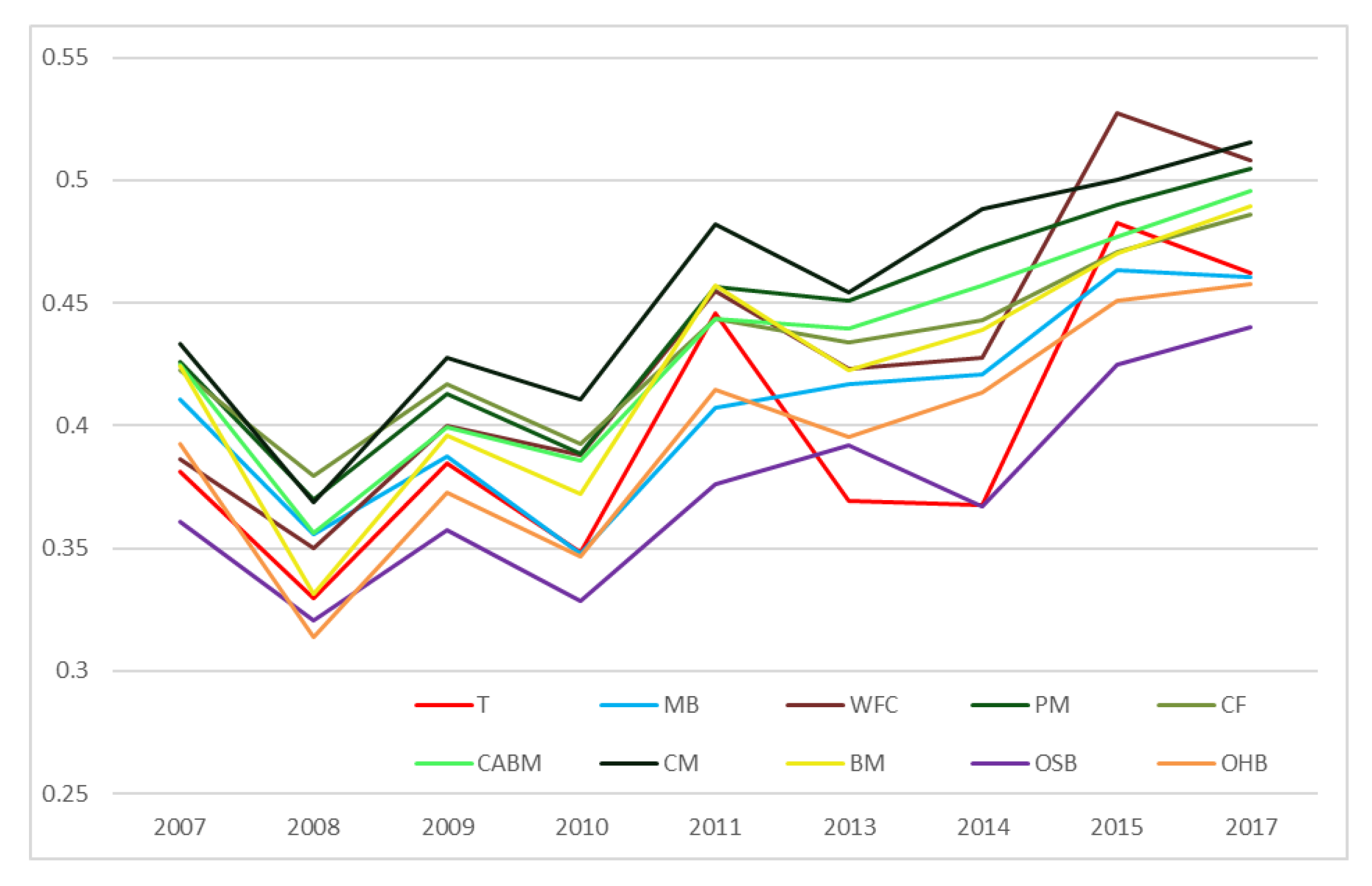
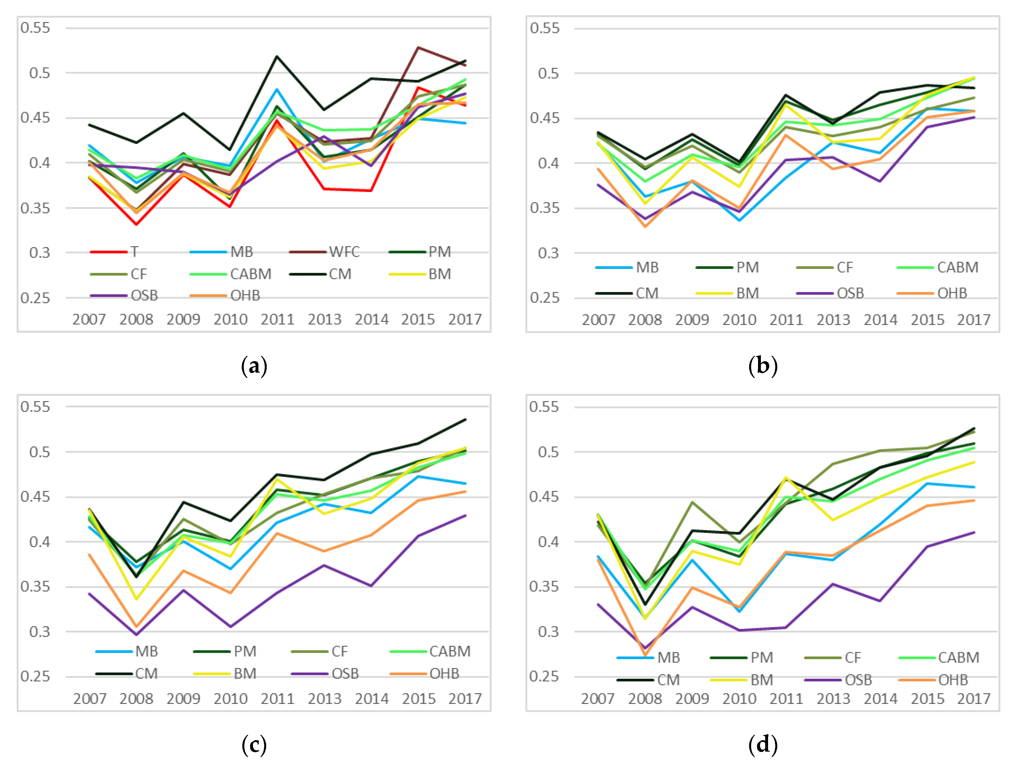
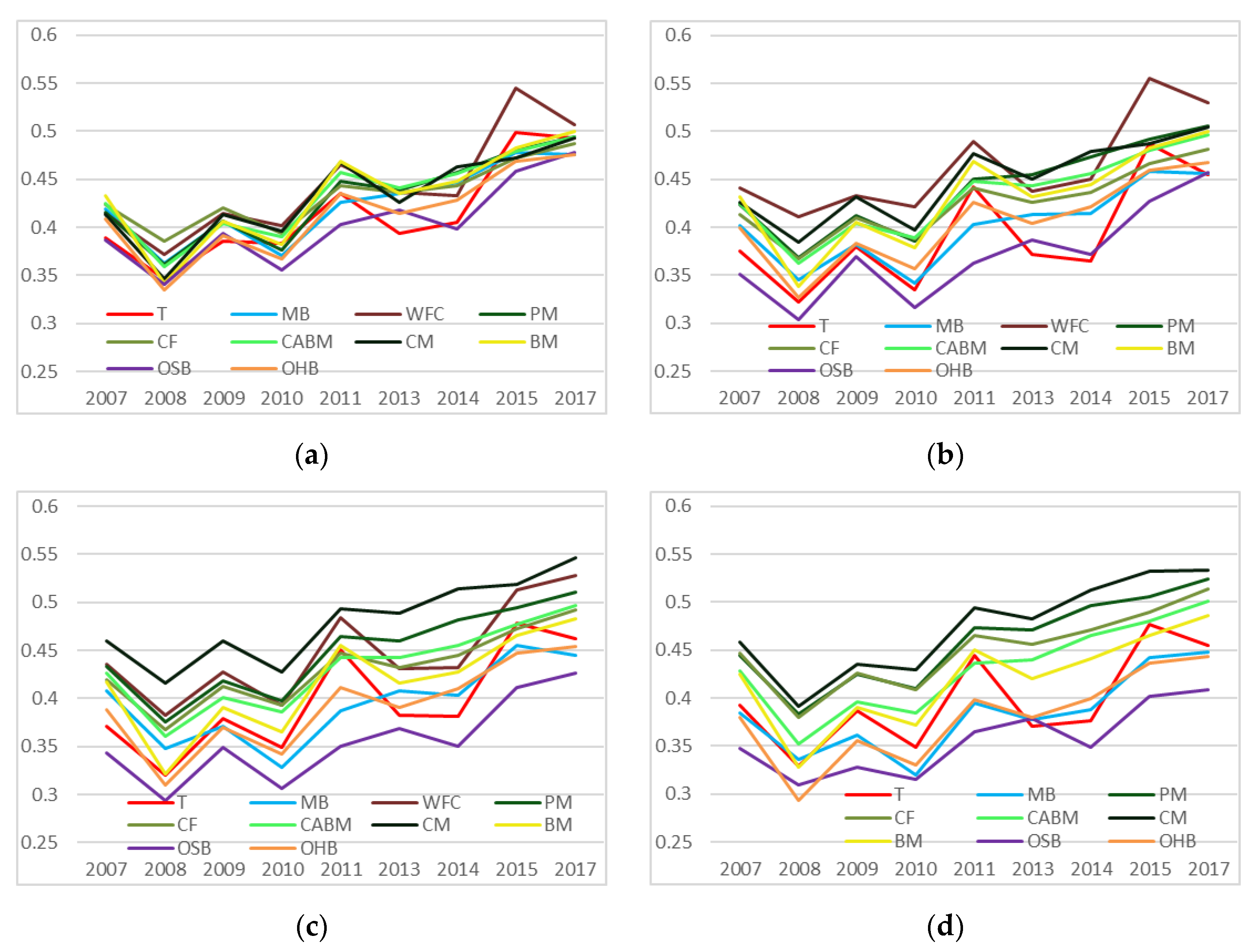
The study of the disaster impact and the post-disaster recovery for different forest types revealed two interesting phenomena. (1) There was a great difference between natural and planted forests in terms of the change in EVI from 2007 to 2017. Natural forests had a rich variety of species and high level of biodiversity, while planted forests were more homogenous, thus planted forests had a lower ability to withstand the disaster than natural forests [56,57,58]. Therefore, in the same elevation zones, planted forests were more severely affected by the ice storm than natural forests. However, human activities changed the natural recovery process. This resulted in the planted forests recovered fast but also produced large fluctuations in the EVI during the process of post-disaster recovery. (2) In the comparative analysis of different forest types in the same elevation zone and slope zone, we found that coniferous forests suffered less EVI decline than broad-leaved forests. This suggests that coniferous forests are more resilient to ice and snow than broad-leaved forests, which might result from broad-leaved forests having broad, flat crowns that expose a large surface area of branches and, therefore, make them more susceptible to extensive damage. In contrast, coniferous trees expose a smaller proportion of their lateral branches to ice accumulation [59,60], resulting in less physical damage than in broad-leaved forests. However, due to their characteristics and the hot, humid climate in Chebaling, broad-leaved forests can photosynthesize faster and thus have a higher rate of recovery.

5. Conclusions

In this study, we used multisource, long-time series remote-sensing data and field-survey data to evaluate the spatial and temporal variations in forest damage and recovery after the 2008 ice storm in Chebaling National Nature Reserve. Firstly, by analyzing the relationship between remotely sensed EVI data and field survey data in Chebaling, we concluded that the annual mean EVI can be used to represent the forest stock volume because of the strong correlation between them and can reflect the status of regional forests and also changes in status. Secondly, the effects of topography and forest types on disaster impact and post-disaster recovery were analyzed from two aspects of single factor and multiple factor, respectively. Our results indicate that topography had a considerable effect on disaster impact and forest recovery, and elevation was more decisive than slope in disaster impact. The disaster impact and recovery degree for all forest types in high-altitude and steep-slope areas were higher than those in low-altitude and gentle-slope areas, especially in the 700–1000 m elevation zones and 25–40° slope zones. However, coniferous forests in the high-elevation zones and steep-slope zones grew better than broad-leaved forests, so the hardest-hit areas for coniferous forests were higher and steeper than that of broad-leaved forests. The disaster analysis for different forest types showed that broad-leaved forests were more affected by the ice storm than coniferous forests but had faster recovery rate and a higher degree of recovery. Although planted forests were more severely affected by the ice storm than natural forests in the areas with similar topographical conditions, the recovery rate for planted forests was faster than that for natural forests because of human intervention. But the recovery process fluctuated greatly. Compared with the areas with monospecific tree species, the recovery process of coniferous and broad-leaved mixed forest is more stable. This study focuses on analyzing the characteristics and laws of disaster impact and post-disaster recovery. In the future, the driving force of forest recovery will be further studied and more experiments will be conducted in bigger scale and more regions to analyze the universality of the characteristics and laws summarized in the study.

References

1. Nehru, P.; Balasubramanian, P. Mangrove species diversity and composition in the successional habitats of Nicobar Islands, India: A post-tsunami and subsidence scenario. For. Ecol. Manag. 2018, 427, 70–77. [Google Scholar] [CrossRef]
2. Fan, N.N.; Nie, R.H.; Wang, Q.; Liu, X.N. Dramatic undercutting of piedmont rivers after the 2008 Wenchuan ms 8.0 earthquake. Sci. Rep. 2016, 6, 37108. [Google Scholar] [CrossRef] [PubMed] [Green Version]
3. Tomppo, E.; Antropov, O.; Praks, J. Boreal forest snow damage mapping using multi-temporal sentinel-1 data. Remote Sens. 2019, 11, 384. [Google Scholar] [CrossRef] [Green Version]
4. Wu, J.S.; Wang, T.; Pan, K.Y.; Li, W.F.; Huang, X.L. Assessment of forest damage caused by an ice storm using multi-temporal remote-sensing images: A case study from guangdong province. Int. J. Remote Sens. 2016, 37, 3125–3142. [Google Scholar] [CrossRef]
5. Zhang, J.D.; Hull, V.; Xu, W.H.; Liu, J.G.; Ouyang, Z.Y.; Huang, J.Y.; Wang, X.Z.; Li, R.G. Impact of the 2008 wenchuan earthquake on biodiversity and giant panda habitat in wolong nature reserve, China. Ecol. Res. 2011, 26, 523–531. [Google Scholar] [CrossRef]
6. Rhoads, A.G.; Hamburg, S.P.; Fahey, T.J.; Siccama, T.G.; Hane, E.N.; Battles, J.; Cogbill, C.; Randall, J.; Wilson, G. Effects of an intense ice storm on the structure of a northern hardwood forest. Can. J. For. Res. 2002, 32, 1763–1775. [Google Scholar] [CrossRef] [Green Version]
7. Markus, R.; Michael, B.; Philippe, C.; Dorothea, F.; Mahecha, M.D.; Seneviratne, S.I.; Jakob, Z.; Christian, B.; Nina, B.; Frank, D.C. Climate extremes and the carbon cycle. Nature 2013, 500, 287–295. [Google Scholar]
8. Weeks, B.C.; Hamburg, S.P.; Vadeboncoeur, M.A. Ice storm effects on the canopy structure of a northern hardwood forest after 8 years. Can. J. For. Res. 2009, 39, 1475–1483. [Google Scholar] [CrossRef] [Green Version]
9. Lind, L.; Nilsson, C.; Weber, C. Effects of ice and floods on vegetation in streams in cold regions: Implications for climate change. Ecol. Evol. 2014, 4, 4173–4184. [Google Scholar] [CrossRef]
10. Jiao, Q.J.; Zhang, B.; Liu, L.Y.; Li, Z.W.; Yue, Y.M.; Hu, Y. Assessment of spatio-temporal variations in vegetation recovery after the Wenchuan earthquake using landsat data. Nat. Hazards 2014, 70, 1309–1326. [Google Scholar] [CrossRef]
11. Zhang, J.D.; Hull, V.; Huang, J.Y.; Yang, W.; Zhou, S.Q.; Xu, W.H.; Huang, Y.; Ouyang, Z.Y.; Zhang, H.M.; Liu, J.G. Natural recovery and restoration in giant panda habitat after the Wenchuan earthquake. For. Ecol. Manag. 2014, 319, 1–9. [Google Scholar] [CrossRef]
12. Lin, C.Y.; Lo, H.M.; Chou, W.C.; Lin, W.T. Vegetation recovery assessment at the jou-jou mountain landslide area caused by the 921 earthquake in central Taiwan. Ecol. Model. 2004, 176, 75–81. [Google Scholar] [CrossRef]
13. Stone, R. Natural disasters-ecologists report huge storm losses in china’s forests. Science 2008, 319, 1318–1319. [Google Scholar] [CrossRef] [PubMed]
14. Shao, Q.Q.; Huang, L.; Liu, J.Y.; Kuang, W.H.; Li, J. Analysis of forest damage caused by the snow and ice chaos along a transect across southern China in spring 2008. J. Geogr. Sci. 2011, 21, 219–234. [Google Scholar] [CrossRef]
15. Shi, L.L. Assessment of forest damage caused by ice storm based on modis data—A case study of Jiangxi Province, China. Disaster Adv. 2013, 6, 67–72. [Google Scholar]
16. Shi, L.L.; Wang, H.M.; Zhang, W.J.; Shao, Q.Q.; Yang, F.T.; Ma, Z.Q.; Wang, Y.D. Spatial response patterns of subtropical forests to a heavy ice storm: A case study in Poyang lake basin, southern China. Nat. Hazards 2013, 69, 2179–2196. [Google Scholar] [CrossRef]
17. Ge, J.L.; Xiong, G.M.; Wang, Z.X.; Zhang, M.; Zhao, C.M.; Shen, G.Z.; Xu, W.T.; Xie, Z.Q. Altered dynamics of broad-leaved tree species in a Chinese subtropical montane mixed forest: The role of an anomalous extreme 2008 ice storm episode. Ecol. Evol. 2015, 5, 1484–1493. [Google Scholar] [CrossRef]
18. Zhou, B.Z.; Wang, X.M.; Cao, Y.H.; Ge, X.G.; Gu, L.H.; Meng, J.L. Damage assessment to subtropical forests following the 2008 Chinese ice storm. Iforest-Biogeosci. For. 2017, 10, 406–415. [Google Scholar] [CrossRef] [Green Version]
19. Hansen, W.J.; CRANSON, J. Spatial analysis of forest damage in central massachusetts resulting from the December 2008 ice storm. Northeast. Nat. 2016, 23, 378–394. [Google Scholar] [CrossRef]
20. Rhoades, R.W.; Stipes, R.J. Ice damage to trees on the Virginia tech campus from ice storms. Northeast. Nat. 2007, 14, 51–60. [Google Scholar] [CrossRef]
21. Lafon, C.W. Ice-storm disturbance and long-term forest dynamics in the adirondack mountains. J. Veg. Sci. 2004, 15, 267–276. [Google Scholar] [CrossRef]
22. Hooper, M.C.; Arii, K.; Lechowicz, M.J. Impact of a major ice storm on an old-growth hardwood forest. Can. J. Bot. 2001, 79, 70–75. [Google Scholar]
23. Rebertus, A.J.; Shifley, S.R.; Richards, R.H.; Roovers, L.M. Ice storm damage to an old-growth oak-hickory forest in Missouri. Am. Midl. Nat. 1997, 137, 48–61. [Google Scholar] [CrossRef]
24. Wang, X.; Huang, S.N.; Li, J.X.; Zhou, G.Y.; Shi, L. Sprouting response of an evergreen broad-leaved forest to a 2008 winter storm in Nanling mountains, southern China. Ecosphere 2016, 7. [Google Scholar] [CrossRef]
25. Bhowmik, A.K.; Cabral, P. Cyclone sidr impacts on the sundarbans floristic diversity. Earth Sci. Res. 2012, 2, 62–79. [Google Scholar] [CrossRef] [Green Version]
26. Hislop, S.; Jones, S.; Soto-Berelov, M.; Skidmore, A.; Haywood, A.; Nguyen, T.H. Using landsat spectral indices in time-series to assess wildfire disturbance and recovery. Remote Sens. 2018, 10, 460. [Google Scholar] [CrossRef] [Green Version]
27. Wilson, N.R.; Norman, L.M. Analysis of vegetation recovery surrounding a restored wetland using the normalized difference infrared index (ndii) and normalized difference vegetation index (ndvi). Int. J. Remote Sens. 2018, 39, 3243–3274. [Google Scholar] [CrossRef] [Green Version]
28. Cai, D.S.; Song, X.J. Bio-resource and protection countermeasure in national reserve of chebaling in Guangdong province. Ecol. Sci. 2005, 24, 282–285. [Google Scholar]
29. Chen, L.; Shu, Z.; Yao, W.; Ma, Y.; Xiao, W.; Huang, X. Combined effects of habitat and interspecific interaction define co-occurrence patterns of sympatric galliformes. Avian Res. 2019, 10, 29. [Google Scholar] [CrossRef] [Green Version]
30. Huete, A.; Didan, K.; Miura, T.; Rodriguez, E.P.; Gao, X.; Ferreira, L.G. Overview of the radiometric and biophysical performance of the modis vegetation indices. Remote Sens. Environ. 2002, 83, 195–213. [Google Scholar] [CrossRef]
31. Liu, H.Q.; Huete, A. A feedback based modification of the ndvi to minimize canopy background and atmospheric noise (vol 33, pg 457, 1995). IEEE Trans. Geosci. Remote Sens. 1995, 33, 457–465. [Google Scholar] [CrossRef]
32. Justice, C.O.; Smith, R.; Gill, A.M.; Csiszar, I. A review of current space-based fire monitoring in australia and the gofc/gold program for international coordination. Int. J. Wildland Fire 2003, 12, 247–258. [Google Scholar] [CrossRef]
33. Woodcock, C.E.; Allen, R.; Anderson, M.; Belward, A.; Bindschadler, R.; Cohen, W.; Gao, F.; Goward, S.N.; Helder, D.; Helmer, E.; et al. Free access to landsat imagery. Science 2008, 320, 1011. [Google Scholar] [CrossRef] [PubMed]
34. Wulder, M.A.; Masek, J.G.; Cohen, W.B.; Loveland, T.R.; Woodcock, C.E. Opening the archive: How free data has enabled the science and monitoring promise of landsat. Remote Sens. Environ. 2012, 122, 2–10. [Google Scholar] [CrossRef]
35. MacDicken, K.G. Global forest resources assessment 2015: What, why and how? For. Ecol. Manag. 2015, 352, 3–8. [Google Scholar] [CrossRef] [Green Version]
36. Jagodzinski, A.M.; Dyderski, M.K.; Gesikiewicz, K.; Horodecki, P. Tree and stand level estimations of abies alba mill. Aboveground biomass. Ann. For. Sci. 2019, 76, 56. [Google Scholar] [CrossRef] [Green Version]
37. Villanova, P.H.; Torres, C.; Jacovine, L.A.G.; Soares, C.P.B.; da Silva, L.F.; Schettini, B.L.S.; da Rocha, S. Prognosis of the diameter distribution and carbon stock in a secondary atlantic forest by markov chain. Rev. Arvore 2018, 42. [Google Scholar] [CrossRef]
38. Ehlers, S.; Saarela, S.; Lindgren, N.; Lindberg, E.; Nystrom, M.; Persson, H.J.; Olsson, H.; Stahl, G. Assessing error correlations in remote sensing-based estimates of forest attributes for improved composite estimation. Remote Sens. 2018, 10, 667. [Google Scholar] [CrossRef] [Green Version]
39. Hawrylo, P.; Wezyk, P. Predicting growing stock volume of scots pine stands using sentinel-2 satellite imagery and airborne image-derived point clouds. Forests 2018, 9, 274. [Google Scholar] [CrossRef] [Green Version]
40. Dos Reis, A.A.; Carvalho, M.C.; de Mello, J.M.; Gomide, L.R.; Ferraz, A.C.; Acerbi, F.W. Spatial prediction of basal area and volume in eucalyptus stands using landsat tm data: An assessment of prediction methods. N. Z. J. For. Sci. 2018, 48, 1. [Google Scholar] [CrossRef] [Green Version]
41. Macedo, F.L.; Sousa, A.M.O.; Goncalves, A.C.; da Silva, J.R.M.; Mesquita, P.A.; Rodrigues, R.A.F. Above-ground biomass estimation for quercus rotundifolia using vegetation indices derived from high spatial resolution satellite images. Eur. J. Remote Sens. 2018, 51, 932–944. [Google Scholar] [CrossRef] [Green Version]
42. Bolton, D.K.; White, J.C.; Wulder, M.A.; Coops, N.C.; Hermosilla, T.; Yuan, X.P. Updating stand-level forest inventories using airborne laser scanning and landsat time series data. Int. J. Appl. Earth Obs. Geoinf. 2018, 66, 174–183. [Google Scholar] [CrossRef]
43. Wolter, P.T.; Mladenoff, D.J.; Host, G.E.; Crow, T.R. Improved forest classification in the northern lake-states using multitemporal landsat imagery. Photogramm. Eng. Remote Sens. 1995, 61, 1129–1143. [Google Scholar]
44. Vieira, I.C.G.; de Almeida, A.S.; Davidson, E.A.; Stone, T.A.; de Carvalho, C.J.R.; Guerrero, J.B. Classifying successional forests using landsat spectral properties and ecological characteristics in eastern Amazonia. Remote Sens. Environ. 2003, 87, 470–481. [Google Scholar] [CrossRef]
45. Sesnie, S.E.; Gessler, P.E.; Finegan, B.; Thessler, S. Integrating landsat tm and srtm-dem derived variables with decision trees for habitat classification and change detection in complex neotropical environments. Remote Sens. Environ. 2008, 112, 2145–2159. [Google Scholar] [CrossRef]
46. Immitzer, M.; Atzberger, C.; Koukal, T. Tree species classification with random forest using very high spatial resolution 8-band worldview-2 satellite data. Remote Sens. 2012, 4, 2661–2693. [Google Scholar] [CrossRef] [Green Version]
47. Ghosh, A.; Joshi, P.K. A comparison of selected classification algorithms for mapping bamboo patches in lower gangetic plains using very high resolution worldview 2 imagery. Int. J. Appl. Earth Obs. Geoinf. 2014, 26, 298–311. [Google Scholar] [CrossRef]
48. Walter, V. Object-based classification of remote sensing data for change detection. Isprs J. Photogramm. Remote Sens. 2004, 58, 225–238. [Google Scholar] [CrossRef]
49. Nitze, I.; Barrett, B.; Cawkwell, F. Temporal optimisation of image acquisition for land cover classification with random forest and modis time-series. Int. J. Appl. Earth Obs. Geoinf. 2015, 34, 136–146. [Google Scholar] [CrossRef] [Green Version]
50. Barrett, B.; Nitze, I.; Green, S.; Cawkwell, F. Assessment of multi-temporal, multi-sensor radar and ancillary spatial data for grasslands monitoring in ireland using machine learning approaches. Remote Sens. Environ. 2014, 152, 109–124. [Google Scholar] [CrossRef] [Green Version]
51. Belgiu, M.; Dragut, L. Random forest in remote sensing: A review of applications and future directions. Isprs J. Photogramm. Remote Sens. 2016, 114, 24–31. [Google Scholar] [CrossRef]
52. Topouzelis, K.; Psyllos, A. Oil spill feature selection and classification using decision tree forest on sar image data. Isprs J. Photogramm. Remote Sens. 2012, 68, 135–143. [Google Scholar] [CrossRef]
53. Zhao, H.; Ma, Y.; Chen, F.; Liu, J.; Yang, J. Monitoring quarry area with landsat long time-series for socioeconomic study. Remote Sens. 2018, 10, 517. [Google Scholar] [CrossRef] [Green Version]
54. Valinger, E.; Lundqvist, L. The Influence of Thinning and Nitrogen Fertilisation on the Frequency of Snow and Wind Induced Stand Damage in Forests. Scott. For. 1992, 46, 311–320. [Google Scholar]
55. Zhu, J.J.; Li, X.F.; Liu, Z.G.; Cao, W.; Gonda, Y.; Matsuzaki, T. Factors affecting the snow and wind induced damage of a montane secondary forest in northeastern China. Silva Fenn. 2006, 40, 37–51. [Google Scholar] [CrossRef] [Green Version]
56. Viani, R.A.G.; Durigan, G.; Melo, A.C.G.D. Natural regeneration under forest plantations: “Green deserts” or milieu for biodiversity? Ciênc Florest 2010, 20, 533–552. [Google Scholar]
57. Onyekwelu, J.C.; Olabiwonnu, A.A. Can forest plantations harbour biodiversity similar to natural forest ecosystems over time? Int. J. Biodivers. Sci. Ecosyst. Serv. Manag. 2016, 12. [Google Scholar] [CrossRef] [Green Version]
58. Christensen, M.; Emborg, J. Biodiversity in natural versus managed forest in Denmark. For. Ecol. Manag. 1996, 85, 47–51. [Google Scholar] [CrossRef]
59. Bruederle, L.P.; Stearns, F.W. Ice storm damage to a southern wisconsin mesic forest. Bull. Torrey Bot. Club 1985, 112, 167–175. [Google Scholar] [CrossRef]
60. Hauer, R.J.; Wang, W.; Dawson, J.O. Ice storm damage to urban trees. J. Arboric. 1993, 19, 1993. [Google Scholar]
Figure 1. The map above represents the location and high-resolution remote-sensing image of Chebaling (the red star represents the central point of Chebaling; the GF-1 remote-sensing image had a resolution of 2 m and was acquired on 15 February 2017); the map below shows the DEM of Chebaling.
Remotesensing 12 00164 g001
Figure 2. (a) Spatial distribution of forest stock volume; (b) spatial distribution of forest types. These maps were derived from forestry sub-compartment data in 2016.
Remotesensing 12 00164 g002
Figure 3. Spatial correlation analysis. (a) Spatial correlation between maximum value of EVI and forest stock volume in 2016; (b) spatial correlation between mean value of EVI and forest stock volume in 2016.
Remotesensing 12 00164 g003
Figure 4. Temporal correlation analysis (2009–2015, excluding 2012). (a) Temporal correlation between maximum value of EVI and forest stock volume; (b) temporal correlation between mean value of EVI and forest stock volume.
Remotesensing 12 00164 g004
Figure 5. (a) Land-use classification map based on GF-1 data; (b) forest-types distribution map derived from forestry sub-compartment data and the land-use classification map.
Remotesensing 12 00164 g005
Figure 6. (a) Spatial distribution of different elevation zones in Chebaling; (b) spatial distribution of different slope zones in Chebaling.
Remotesensing 12 00164 g006
Figure 7. Broken-line graph showing EVI changes from 2007 to 2017 in different elevation zones.
Remotesensing 12 00164 g007
Figure 8. Broken-line graph showing EVI changes from 2007 to 2017 in different slope zones.
Remotesensing 12 00164 g008
Figure 9. Broken-line graph showing EVI changes from 2007 to 2017 for different forest types.
Remotesensing 12 00164 g009
Figure 10. Broken-line graph showing EVI changes for 10 forest types, from 2007 to 2017, in four elevation zones: (a) 400–500 m; (b) 500–600 m; (c) 600–700 m; and (d) 700–800 m.
Remotesensing 12 00164 g010
Figure 11. Broken-line graph showing EVI changes for 10 forest types, from 2007 to 2017, in typical slope zones: (a) 10–15°; (b) 15–20°; (c) 20–25°; and (d) 25–30°.
Remotesensing 12 00164 g011
Figure 12. Broken-line graph showing EVI changes from 2007 to 2017, in all elevation zones, for six forest types: (a) CF; (b) PM; (c) CM; (d) CABM; (e) BM; and (f) OHB.
Remotesensing 12 00164 g012
Figure 13. Broken-line graph showing EVI changes from 2007 to 2017, in all slope zones, for six forest types: (a) CF; (b) PM; (c) CM; (d) CABM; (e) BM; and (f) OHB.
Remotesensing 12 00164 g013aRemotesensing 12 00164 g013b