Retrieval of NO₂ Column Amounts from Ground-Based Hyperspectral Imaging Sensor Measurements

Abstract

Total column amounts of NO₂ (TCN) were estimated from ground-based hyperspectral imaging sensor (HIS) measurements in a polluted urban area (Seoul, Korea) by applying the radiance ratio fitting method with five wavelength pairs from 400 to 460 nm. We quantified the uncertainty of the retrieved TCN based on several factors. The estimated TCN uncertainty was up to 0.09 Dobson unit (DU), equivalent to 2.687 × 10²⁰ molecules m⁻²) given a 1° error for the observation geometries, including the solar zenith angle, viewing zenith angle, and relative azimuth angle. About 0.1 DU (6.8%) was estimated for an aerosol optical depth (AOD) uncertainty of 0.01. In addition, the uncertainty due to the NO2 vertical profile was 14% to 22%. Compared with the co-located Pandora spectrophotometer measurements, the HIS captured the temporal variation of the TCN during the intensive observation period. The correlation between the TCN from the HIS and Pandora also showed good agreement, with a slight positive bias (bias: 0.6 DU, root mean square error: 0.7 DU).

1. Introduction

Nitrogen dioxide (NO₂) plays a crucial role in catalytic cycles of reactions for ozone depletion in the stratosphere and is a precursor to ozone formation in the troposphere [1,2]. In addition, NO₂ also significantly affects local instantaneous radiative forcing by the absorption of solar radiation [3] and is related to the air quality in the troposphere (e.g., [4,5,6]).

Ground-based spectrometers, such as the Pandora spectrophotometer (e.g., [7,8]), Brewer spectrophotometer (e.g., [9,10]), and multi-axis differential optical absorption spectroscopy (DOAS) (e.g., [11,12]), have been used to estimate total and tropospheric column amounts of NO₂. The products of ground-based spectrometers have been utilized not only to monitor the distribution and variation of NO₂ for air quality but also to validate satellite products, such as the Scanning Imaging Absorption Spectrometer for Atmospheric Chartography (SCIAMACHY), ozone monitoring instrument (OMI), and tropospheric monitoring instrument (TropOMI), in many previous studies [13,14,15,16,17].

Korea has various emission sources of NO₂ and a distinct diurnal variation due to anthropogenic emissions and photochemical reactions [18]. Campaigns have been executed to understand the distribution and variation of total column amounts of trace gases, including NO₂, in Korea using the Pandora spectrophotometer during the Distributed Regional Aerosol Gridded Observation Networks (DRAGON)-North East Asia [19,20], Megacity Air Pollution Studies-Seoul (MAPS-Seoul) [18,21], and Korea–US Air quality study (KORUS-AQ) [22,23] in 2012, 2015, and 2016, respectively. Since the conclusion of the KORUS-AQ campaign, two of the Pandora spectrophotometers have been in operation in Seoul and Busan.

A limited number of optical instruments are operated to cover the regions with high concentrations of NO₂ in Korea. Therefore, it is necessary to utilize several kinds of optical instruments to supplement the spatial coverage of the Pandora spectrophotometer observation network. In this study, we retrieved the total column amount of NO₂ (hereafter, TCN) from spatial and spectral radiance information from ground-based hyperspectral imaging sensor (HIS) measurements in Seoul, Korea.

An overview of the instruments, including the HIS, is given in Section 2. A detailed explanation of the algorithm for the TCN, with a sensitivity analysis and uncertainty estimations with respect to the observation geometries, aerosol optical depth (AOD), and NO₂ vertical profile, are provided in Section 3. Finally, a comparison of the TCN from the HIS with that from the Pandora spectrophotometer measurements is presented in Section 4.

2. Measurements

2.1. Site

The HIS (UV-VIS hyperspectral spectrophotometer, Headwall Photonics Inc., Bolton, MA, USA) was operated side-by-side with the Pandora spectrophotometer and CIMEL sun/sky radiometer at Yonsei University (37.564°N, 126.934°E and 181 m above the mean sea level) in Seoul, Korea. The instruments were located on the rooftop of the science building.

The temporal variation of NO₂ at Yonsei University has been measured by the Pandora spectrophotometer since 2012. The mean tropospheric NO₂ was 1.49 ± 0.65 DU during the MAPS-Seoul campaign (Chong et al., 2018), and the mean total column of NO₂ was 1.2 ± 0.8 DU for 8 years. Considering that there are no point emission sources near the station, and the distance between traffic road and the station is about 300 m, the spatial variation of NO₂ is not as large as the temporal variation.

2.2. Hyperspectral Imaging Sensor (HIS)

The HIS measures scattered shortwave radiance through horizontal scanning, and the scanning schedule was planned to look upward near the sun and not be interfered with by any obstacles in the total field-of-view (FOV). The HIS has a diffraction grating, and light entering through a slit is dispersed and projected onto a 2-D charged-coupled device. The effects for keystone and smile distortion are corrected. The spectral range of the HIS is 250 to 500 nm, with a spectral resolution of 1.4 nm (FWHM; full width at half maximum) and a sampling interval of 0.26 nm (961 bands). The field-of-view is 13° (1392 pixels) in the vertical direction (see details in [24]). Detailed specifications of the HIS are summarized in

Table 1. Specifications of the hyperspectral imaging sensor (HIS) and Pandora spectrophotometer.

	Hyperspectral Imaging Sensor (HIS)	Pandora Spectrophotometer
Wavelength (nm)	250–500	280–525
Spectral sampling (nm)	0.26	0.23
Spectral resolution (FWHM) (nm)	1.4	0.6
Field-of-view	13° (vertical)	1.6°
Detector	Charge-Coupled Device

.

For horizontal scanning, the HIS was mounted on the external horizontal moving plate system. The pan and tilt angles, motion speed of the mounting system, and exposure time of the HIS were controlled by the operating software. Information on the scan positions was automatically recorded in each observation dataset. Geometries between the HIS and the sun were estimated from the above information on the scan position. One dataset included the horizontally scanned radiance within two minutes, and the radiance data were corrected by radiometric and dark calibrations after observation. The radiometric calibration was done with radiometric sensitivity files of the instrument, and dark correction used the dark radiances measured before and after observation. In this study, 28 measured datasets on 30 and 31 October 2017 were used to retrieve the TCN. With spatially resolved TCNs, we retrieved the mean and standard deviation of TCNs as a representative value from each dataset for comparison with the Pandora spectrophotometer.

2.3. Pandora Spectrophotometer (No. 27)

The Pandora spectrophotometer (hereafter, Pandora) is a passive UV-visible hyperspectral sensor with a two-dimensional charge-coupled device (CCD) with a 1.6° FOV. The spectral resolution and its sampling interval are 0.6 (FWHM) and 0.23 nm, respectively. The spectrometer in the control box is connected from the sensor head by a fiber optic cable, and the temperature of the control box is maintained (20 ± 1 °C) to stabilize of the spectrometer (e.g., [7,25]).

Pandora at Yonsei University has been operated since 2012 [18,20]. From the direct sun measurements, the TCN from Pandora is calculated by radiance fitting using the spectral window of 370 to 500 nm [7]. The TCN data with approximately two-minute intervals are provided on the Pandonia Global Network (PGN) website. In this study, we used level 3 TCN data qualified with thresholds of less than 0.05 for the normalized root mean square error (RMSE) of spectral fitting residuals and 0.05 DU for the uncertainties for the TCN retrieval [8].

3. Estimation of Total Column Nitrogen Dioxide (TCN)

3.1. Algorithm Development

The UVSPEC radiative transfer model, which is part of the calculation tool in the radiation model package, libRadtran [26], was used to simulate the radiance in the UV and visible spectral range under various atmospheric conditions. The accuracy of the libRadtran has been proven for simulating UV irradiance and used in numerous studies (http://www.libradtran.org). The only input parameters related to the absorption and scattering characteristics of NO₂ and aerosol (e.g., vertical profile, absorption cross-section for NO₂, and scattering coefficients and phase function for aerosols) determine the fundamental accuracy of the RTM simulation. The U.S. standard atmosphere [27] and extraterrestrial spectra with a 0.1 nm resolution [28] were used for the atmospheric conditions and solar irradiance dataset, respectively. The radiance was simulated with a 0.26 nm sampling interval after adopting a spectral weighting function with a Gaussian distribution with 1.4 nm (FWHM) to describe the instrument specification of the HIS (Table 1). The absorption cross-section for NO₂ was taken considering the temperature dependence [29]. Although several sources are in the stratosphere [1,30], most of the emission sources of NO₂ are located near the surface of the polluted urban area. In this study, we considered the variation of NO₂ concentrations below the 4 km altitude in the simulation. The surface albedo in the RTM is assumed to be 0.1, which can be used for the urban surface conditions [31]. With the conditions for the RTM set as above, the look-up table (LUT) for the algorithm was comprised of observation geometries (solar zenith angle (SZA), viewing zenith (VZA), and relative azimuth angle (RAA)), AOD, and TCN with each discrete interval as summarized in

Table 2. Dimensions of the radiative model simulations.

Variables	Entries	No. of Entries
SZA (°)	0, 10, 20, 30, 40, 50, 60, 70	8
VZA (°)	0, 5, 10, 15, 20, 25, 30, 35, 40, 45, 50, 55, 60, 65, 70	15
RAA (°)	0, 10, 20, 30, 40, 50, 60, 90, 120, 180	10
AOD (550 nm)	0.0, 0.2, 0.4, 0.6, 0.8, 1.0, 1.2, 1.4, 1.6, 1.8, 2.0	11
TCN (DU)	0.1–9.0 (0.1 DU interval)	90

.

Considering the relatively coarse spectral resolution of the HIS and the status were calibrated 2 years before, the differential optical absorption spectroscopy (DOAS) method was carefully excluded. To reduce an effect, which could be caused by the absence of spectral and absolute radiance calibration just before the measurements, the fitting method with radiance ratios between the observations and simulations (e.g., [32]) was applied for TCN retrieval. In addition, the radiances of each wavelength were averaged around the center to reduce a possible wavelength shift effect, and the sensitivity analysis about the number of averaging pixels is discussed in Section 3.2. Five wavelength pairs were used, as shown in

Table 3. Wavelength pairs used in the retrieval of total column amounts of NO₂ (TCN).

$\mathbf{Channel}\left(\mathit{k}\right)$	Strong (I)/Weak (I′) Absorption Wavelength (nm)
1	400.610/407.055
2	409.403/416.598
3	421.661/426.457
4	435.251/442.179
5	448.307/456.834

. The absorption of other trace gases is insignificant compared to the absorption of NO₂ at five wavelength pairs. Each wavelength pair was selected on the location at which the radiance is strongly and weakly absorbed by NO₂, based on the difference in the normalized radiance (which was calculated by dividing the radiance by the irradiance).

The TCN was retrieved from each pixel when the cost function was the smallest. The cost function was defined as ${\chi }^2$, as shown in Equation (1):

$${\chi }^2={{\displaystyle \sum }}_{k=1}^5\frac{{\left(R_{ob{s}_k}-R_{RT{M}_k}\right)}^2}{R_{RT{M}_k}},\left(k=1,2,\dots ,5\right),$$

(1)

where $R_{ob{s}_k}$ and $R_{RT{M}_k}$ are the radiance ratios calculated from the observations and the RTM simulations, respectively. The subscript k indicates the spectral channel as shown in Table 3.

The radiance ratio ($R_k$) was defined by Equation (2):

$$R_k=\frac{{I^{\prime }}_k}{I_k},$$

(2)

where $I_k$ and ${I^{\prime }}_k$ respectively indicate the radiance at the wavelengths for strong and weak NO₂ absorption.

The averaged radiance over the given spectral range, $\mathsf{\Delta }\lambda$, $I_k({I^{\prime }}_k$), was averaged by Equation (3):

$$I_k=\frac{1}{2\mathsf{\Delta }\lambda }{{\displaystyle \int }}_{\lambda -\mathsf{\Delta }\lambda }^{\lambda +\mathsf{\Delta }\lambda }I\left(\lambda \right) d\lambda .$$

(3)

The $R_{RTM}$ was determined from the LUT based on the observation conditions (e.g., SZA, RAA, VZA, and AOD). For the calculation of ${\chi }^2$, the $R_{obs}$ was fitted to $R_{RTM}$ for each of the 0.1 DU TCN intervals. The TCN was estimated when the difference between the observation and simulation was minimized.

3.2. Pixel Co-Adding

Prior to applying the algorithm to the HIS data, the sensitivity of two factors—pixel co-adding and the RAA limitation—was quantified. In many algorithms, pixel co-adding has been used to reduce radiometric random noise (e.g., [33,34]); however, signal intensities in the retrieval process change according to the number of co-adding pixels. Therefore, the optimal numbers of spectral and spatial co-adding pixels were determined through a sensitivity analysis based on the HIS dataset. For the sensitivity of the spectral co-adding, a case study of 11:55–11:57 LST on 30 October 2017 was used. The retrieved TCNs from the HIS were 1.5 ± 0.3 DU, 1.5 ± 0.4 DU, and 1.6 ± 0.7 DU, respectively, when 5, 15, and 25 pixels were spectrally co-added. The deviation of the TCN was enhanced with the increasing number of spectrally co-added pixels, although the mean TCN showed similar values because the absorption spectrum of NO₂ is smoothed by the spectral co-adding, resulting in a large variance. Therefore, five pixels were selected for the spectral co-adding in this study.

Similarly, the sensitivity analysis for the spatial co-adding was executed along the horizontal direction (i.e., RAA axis). Figure 1 shows the normalized standard deviation of the TCN (standard deviation ($\mathsf{\sigma }$) divided by the mean TCN (μ)), by changing the number of spatial co-adding pixels. The mean value of $\mathsf{\sigma }/\mathsf{\mu }$ is 27.3%, 22.8%, 18.6%, 18.6%, and 18.9% for 5, 15, 30, 45, and 60 pixels, respectively. The number of spatial co-adding pixels was determined when the difference of the mean, $\mathsf{\sigma }/\mathsf{\mu }$, was not sensitive to the number of co-adding pixels. Despite similar sensitivities, 45 and 60 pixels were excluded to keep up the spatial resolution of the TCN for the horizontal direction. Based on the sensitivity analysis above, 30 pixels were selected for spatial co-adding.

3.3. Bias Near the Sun

Figure 2 shows the false-color images with arbitrarily selected red green and blue (RGB) wavelengths (R: 500 nm, G: 450 nm, B: 380 nm) and the retrieval results of the TCNs from the HIS, considering the retrieval limitation for the RAA. As shown in Figure 2a,d, the false-color image of the HIS, unexpected biases are found near the sun (i.e., small RAA), and the retrieved TCNs in small RAA pixels are systematically larger than those in large RAA pixels (Figure 2b,e). These non-linear increases of the radiance in all wavelength ranges can be caused by the smearing effect. Smear occurs mainly in bright spots where stray photons can arrive in the register. The smearing effect of the instrument near the sun (i.e., close to the saturation region) caused large bias of the radiance and, consequently, the TCN.

To consider the smearing effect along with the solar disk, we retrieved the TCN in which the RAA was larger than 15° to reduce the RAA dependency in the retrieval. The mean TCNs at 13:39–13:41 LST on 30 October 2017 changed from 1.5 DU to 1.2 DU (−20.0%) by applying an RAA limitation of 15° (Figure 2c). In another case of 12:07–12:09 LST on 31 October 2017, the mean TCN was reduced from 2.7 DUs to 2.1 DUs (−22.2%) for an RAA limitation of 15° (Figure 2f). The retrieved mean TCNs decreased by 12.2% on average when the RAA was limited to larger than 15°.

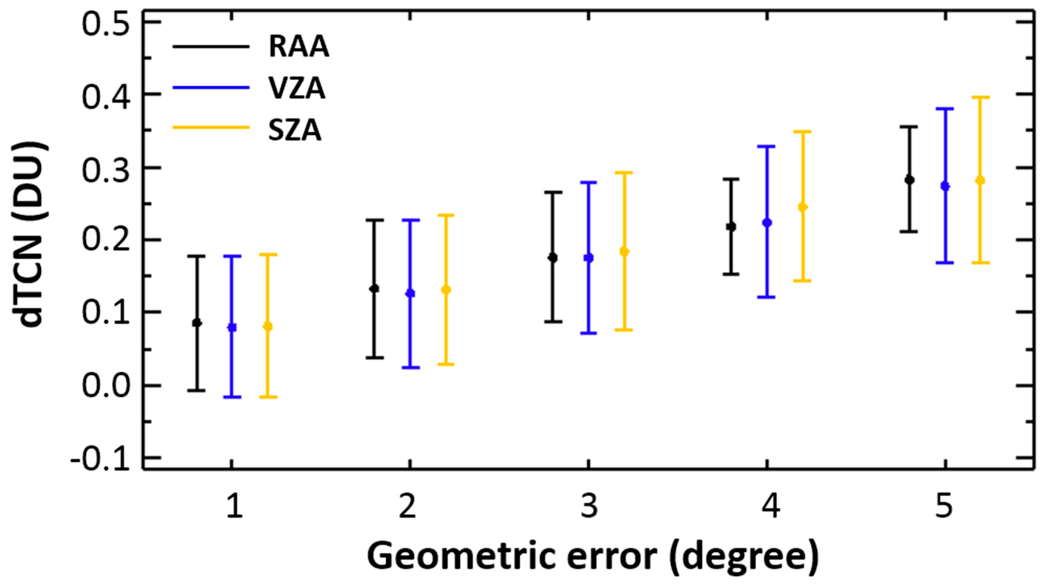
3.4. Uncertainty Estimation

The inherent errors of the instruments and input values used in the fitting process cause the uncertainties in the retrieved TCN. In this section, we quantified the uncertainties caused by the three factors used as input values. In the TCN retrieval algorithm, geometries between the sun and the HIS were calculated by the solar position and recorded dataset for the scan position of the HIS. The bias of the retrieved TCN could be generated by the error of the estimated observation geometries, because the observation geometries determine the path of the sunlight. Figure 3 shows the uncertainty of the TCN with respect to the arbitrary error of geometry. When the SZA, VZA, and RAA have arbitrary measurement errors of 1°, the differences in the TCNs from the reference TCNs (i.e., dTCNs) are 0.08, 0.08, and 0.09 DU, respectively, and the dTCNs are 0.28, 0.27, and 0.28 DU at geometric errors of 5°, respectively. With a geometric error range of 1° to 5°, the TCN can be retrieved with uncertainties from 4.9% to 16.7% for the SZA, from 4.7% to 16.8% for the VZA, and from 5.0% to 18.0% for the RAA; however, the retrieval error of the TCN is insignificant within a geometric error of 1°.

During the intensive observation period, the AOD at 550 nm was obtained from the CIMEL sun/sky radiometer, and the accuracy of the AOD is assumed to be 0.01 [35]. As the mean AOD of the period in this study was 0.12, for the low AOD cases, we estimated the uncertainty of the retrieved TCN about the CIMEL accuracy of 0.01. The TCN was retrieved using the closest AOD value with an LUT bin to exclude errors caused by AOD interpolation. The uncertainty of the retrieved TCN was estimated to be 0.1 DU (6.8%). For the same geometric conditions, the change in the radiance ratio (R) was constant for the TCN change; however, the R is more sensitive to the AOD than to the TCN, especially when the AOD is small. Therefore, the retrieved TCN has relatively large uncertainty caused by the AOD.

The U.S. standard atmospheric condition, used in this study, describes the NO₂ number density up to 120 km and has NO₂ concentration peaks at the stratosphere and troposphere, respectively. Because the variation of total column NO₂ is scaled at all layers in the RTM, the overestimation could be generated at the upper atmosphere. To avoid an unrealistic increase of the NO₂ concentration at the stratosphere, we utilized the concept of the constraint layer. The NO₂ vertical distribution assumes that the NO₂ concentration is only changed within 4 km altitudes based on the profile of the U.S. standard atmospheric conditions (hereafter, the constraint layer). The effective optical path length for the NO₂ absorption is significantly related to its vertical distribution when the instrument measures scattered solar radiation. Therefore, the difference in the NO₂ vertical profile is a considerable factor for the uncertainty analysis of the TCN retrieval from HIS measurements. The uncertainty estimation of the various constraint layer, 1, 2, and 4 km altitudes, is shown in Figure 4.

Figure 4 is an example of the retrieved TCN at 11:38–11:40 LST on 30 October 2017, assuming a constraint layer of 4 (Figure 4a), 2 (Figure 4b), and 1 km (Figure 4c). When the constraint layer for the NO₂ profile changed from 4 to 2 km and from 4 to 1 km, the TCNs increased by 0.2 DU (13%) and 0.3 DU (19%), respectively. For all observation cases, the differences in the TCN were +14% and +22% on average when the constraint layer changed from 4 to 2 km and from 4 to 1 km, respectively. By changing the constraint layer, the radiance intensity at strong absorption wavelengths has a larger sensitivity than those at weak absorption wavelengths for all wavelength pairs. Therefore, the $R_{RTM}$ in the same conditions decreases as the constraint layer changes from 4 km to 2 or 1 km, and it causes a positive bias in the retrieved TCN value. The constraint layer sensitivity only shows the linear increase or decrease in the retrieved TCNs, as shown in Figure 4.

4. Comparison with Co-Located Pandora Measurements

Figure 5a,b shows the time series of the TCN from the HIS (RAA > 15°) and Pandora on 30 and 31 October 2017. From Pandora, the TCN peak appeared between 11:00 and 12:00 LST on 30 October and decreased gradually. Despite the relatively small diurnal variation, the TCN retrieved from the HIS showed a coincidence in the temporal variation of the TCN with Pandora. On 31 October, the TCN has a large diurnal variation of about 2DU. The TCN from the HIS also captures the temporal variation of the TCN on that day. Although the TCN retrieved from the HIS (1.8 ± 0.5 DU) in two days is slightly higher than that of Pandora (1.1 ± 0.5 DU), the TCN from the HIS could be useful to detect the diurnal variation qualitatively, considering the positive bias.

Figure 5c shows the scatterplot of TCN from Pandora and the HIS. For the comparison, the data were selected within 1 minute for the observation time difference between the HIS and Pandora. The bias of the TCN from the HIS and Pandora was 0.6 DU with an RMSE of 0.7 DU (r = 0.84). Most previous studies on optical remote sensing, especially the Pandora, compared ground-based measured NO₂ with satellite products. For example, the TCN between Pandora and the OMI showed ranges of correlation coefficients from 0.50 to 0.82 [36] at Seoul, Korea and from 0.44 to 0.73 [7] at Goddard Space Flight Center (GSFC) depending on the SZA, AOD, and cloud amounts. For the comparison between direct ground-based measurements, the correlation coefficient (r) of TCNs between Pandora and multifunction DOAS (MF-DOAS) was 0.88 [37]. In the comparison between the scattering optical sensor and an in-situ gas analyzer, differential slant column densities of NO₂ measured by scattered sunlight of an Imaging-DOAS instrument showed an agreement of 40% in Beijing [38]. In this study, the different retrieval methods between the HIS (radiance fitting method) and Pandora (DOAS-based method) can cause the discrepancy in the retrieved TCN. Especially, due to the location of the site within the urban area, there could be spatial variability in the NO₂ distribution, which also depends on the meteorology. Thus, different observation methods, i.e., scattered (HIS) and direct (Pandora) radiances, also contributed to the discrepancy. The systematic biases are able to be affected not only by hardware limitations (e.g., possibility of the shift of wavelength and absolute radiance) but also by the algorithm itself (especially, input parameters describing the characteristics and distribution of NO₂ and aerosols, e.g., NO₂ profile, smoothing of the cross-section of NO₂ caused by spectral averaging, aerosol profile, scattering coefficients, and phase function). Despite the overestimation and uncertainty described in Section 3.3, the comparison result is consistent with the results from above previous studies.

5. Summary and Conclusions

The retrieval algorithm for TCN was developed using the HIS ground-based measurements. Based on the spectral sensitivity of NO₂ absorption, the fitting method using the radiance ratios from five wavelength pairs was used to retrieve TCN from the scattered radiance. Due to the limitation of the smearing effect near the solar disk, only the pixels where the RAA is larger than 15° were used as valid results.

The uncertainty was also respectively estimated by the observation geometries, AOD, and the assumed NO₂ vertical profile in the algorithm. The retrieval uncertainty was up to 0.09 DU due to an arbitrary observation geometric error of 1°. For an AOD accuracy of 0.01, the uncertainty of TCN was 0.1 DU (6.8%). Regarding the NO₂ vertical profile, when the constraint layer was changed from 4 to 1 km, the retrieved TCN showed a difference of 14% to 22% from the reference TCN. The radiance ratios with different constraint layers were significantly changed for the same TCNs due to the effective optical path length.

The TCN from the HIS agrees with the temporal variation of that from the Pandora co-located at Yonsei University in Seoul, Korea during the intensive observation period. The bias and the RMSE between the HIS and Pandora were 0.6 and 0.7 DU, respectively. Although the TCN from the HIS has overestimations, the comparison results showed that the retrieval algorithm for the HIS, developed in this study, could be utilized for TCN estimation from ground-based measurements.

In this study, climatology values for the aerosol vertical profiles and aerosol optical properties were used and assumed as a well-mixed profile. In addition, the U.S. standard atmosphere condition limited to changes in NO₂ concentration only below the constraint layer was assumed. In reality, however, shape and spatial variability of aerosol and NO₂ exist in the FOV of the instrument, which can affect the retrievals. The assumption of aerosol and NO₂ should be improved with a realistic database to improve the NO₂ products from the HIS. Furthermore, precise calibration of the spectral shift and absolute radiance will be expected to reduce biases from hardware problems. Based on the above improvements, we expect that the TCN retrieval algorithm can be expanded to airborne measurements by adding several considerations related to the optical properties of the surface and aerosols.

References

1. Crutzen, P.J. The Role of NO and NO2 in the Chemistry of the Troposphere and Stratosphere. Annu. Rev. Earth Planet. Sci. 1979, 7, 443–472. [Google Scholar] [CrossRef]
2. Seinfeld, J.H.; Pandis, S.N. Atmospheric Chemistry and Physics: From Air Pollution to Climate Change; John Wiley & Sons: Hoboken, NJ, USA, 2016. [Google Scholar]
3. Solomon, S.; Portmann, R.W.; Sanders, R.W.; Daniel, J.S.; Madsen, W.; Bartram, B.; Dutton, E.G. On the role of nitrogen dioxide in the absorption of solar radiation. J. Geophys. Res. Atmos. 1999, 104, 12047–12058. [Google Scholar] [CrossRef]
4. Seinfeld, J.H. Ozone Air Quality Models. JAPCA 1988, 38, 616–645. [Google Scholar] [CrossRef] [PubMed]
5. Choi, Y.; Wang, Y.; Zeng, T.; Cunnold, D.; Yang, E.-S.; Martin, R.; Chance, K.; Thouret, V.; Edgerton, E. Springtime transitions of NO2, CO, and O3 over North America: Model evaluation and analysis. J. Geophys. Res. Atmos. 2008, 113, D20311. [Google Scholar] [CrossRef]
6. Choi, Y.; Kim, J.; Eldering, A.; Osterman, G.; Yung, Y.L.; Gu, Y.; Liou, K.N. Lightning and anthropogenic NOx sources over the United States and the western North Atlantic Ocean: Impact on OLR and radiative effects. Geophys. Res. Lett. 2009, 36, L17806. [Google Scholar] [CrossRef] [Green Version]
7. Herman, J.; Cede, A.; Spinei, E.; Mount, G.; Tzortziou, M.; Abuhassan, N. NO2 column amounts from ground-based Pandora and MFDOAS spectrometers using the direct-sun DOAS technique: Intercomparisons and application to OMI validation. J. Geophys. Res. Atmos. 2009, 114, D13307. [Google Scholar] [CrossRef] [Green Version]
8. Tzortziou, M.; Herman, J.R.; Cede, A.; Loughner, C.P.; Abuhassan, N.; Naik, S. Spatial and temporal variability of ozone and nitrogen dioxide over a major urban estuarine ecosystem. J. Atmos. Chem. 2015, 72, 287–309. [Google Scholar] [CrossRef]
9. Brewer, A.W. A replacement for the Dobson spectrophotometer? Pure Appl. Geophys. 1973, 106–108, 919–927. [Google Scholar] [CrossRef]
10. Kerr, J.B. New methodology for deriving total ozone and other atmospheric variables from Brewer spectrophotometer direct sun spectra: New methodology using brewer direct sun spectra. J. Geophys. Res. Atmos. 2002, 107, 4731. [Google Scholar] [CrossRef]
11. Hönninger, G. Multi axis differential optical absorption spectroscopy. Atmos. Chem. Phys. 2004, 24, 231–254. [Google Scholar] [CrossRef] [Green Version]
12. Irie, H.; Takashima, H.; Kanaya, Y.; Boersma, K.F.; Gast, L.; Wittrock, F.; Brunner, D.; Zhou, Y.; Van Roozendael, M. Eight-component retrievals from ground-based MAX-DOAS observations. Atmos. Meas. Tech. 2011, 4, 1027–1044. [Google Scholar] [CrossRef] [Green Version]
13. Ionov, D.; Goutail, F.; Pommereau, J.-P.; Bazureau, A.; Kyro, E.; Portafaix, T.; Held, G.; Ericksen, P.; Dorokhov, V. Ten years of NO2 comparisons between ground-based SAOZ and satellite instruments (GOME, SCIAMACHY, OMI). In Proceedings of the Atmospheric Science Conference, Frascati, Italy, 8–12 May 2006. [Google Scholar]
14. Celarier, E.A.; Brinksma, E.J.; Gleason, J.F.; Veefkind, J.P.; Cede, A.; Herman, J.R.; Ionov, D.; Goutail, F.; Pommereau, J.-P.; Lambert, J.-C.; et al. Validation of Ozone Monitoring Instrument nitrogen dioxide columns. J. Geophys. Res. 2008, 113. [Google Scholar] [CrossRef] [Green Version]
15. Wenig, M.O.; Cede, A.M.; Bucsela, E.J.; Celarier, E.A.; Boersma, K.F.; Veefkind, J.P.; Brinksma, E.J.; Gleason, J.F.; Herman, J.R. Validation of OMI tropospheric NO2 column densities using direct-Sun mode Brewer measurements at NASA Goddard Space Flight Center. J. Geophys. Res. 2008, 113. [Google Scholar] [CrossRef]
16. Kramer, L.J.; Leigh, R.J.; Remedios, J.J.; Monks, P.S. Comparison of OMI and ground-based in situ and MAX-DOAS measurements of tropospheric nitrogen dioxide in an urban area. J. Geophys. Res. 2008, 113, D16S39. [Google Scholar] [CrossRef]
17. Griffin, D.; Zhao, X.; McLinden, C.A.; Boersma, F.; Bourassa, A.; Dammers, E.; Degenstein, D.; Eskes, H.; Fehr, L.; Fioletov, V.; et al. High-Resolution Mapping of Nitrogen Dioxide With TROPOMI: First Results and Validation Over the Canadian Oil Sands. Geophys. Res. Lett. 2019, 46, 1049–1060. [Google Scholar] [CrossRef] [Green Version]
18. Chong, H.; Lee, H.; Koo, J.-H.; Kim, J.; Jeong, U.; Kim, W.; Kim, S.-W.; Herman, J.R.; Abuhassan, N.K.; Ahn, J.; et al. Regional Characteristics of NO2 Column Densities from Pandora Observations during the MAPS-Seoul Campaign. Aerosol Air Qual. Res. 2018, 18, 2207–2219. [Google Scholar] [CrossRef] [Green Version]
19. Baek, K.; Kim, J.H.; Herman, J.R.; Haffner, D.P.; Kim, J. Validation of Brewer and Pandora measurements using OMI total ozone. Atmos. Environ. 2017, 160, 165–175. [Google Scholar] [CrossRef]
20. Kim, J.; Kim, J.; Cho, H.-K.; Herman, J.; Park, S.S.; Lim, H.K.; Kim, J.-H.; Miyagawa, K.; Lee, Y.G. Intercomparison of total column ozone data from the Pandora spectrophotometer with Dobson, Brewer, and OMI measurements over Seoul, Korea. Atmos. Meas. Tech. 2017, 10, 3661–3676. [Google Scholar] [CrossRef] [Green Version]
21. Park, J.; Lee, H.; Kim, J.; Herman, J.; Kim, W.; Hong, H.; Choi, W.; Yang, J.; Kim, D. Retrieval Accuracy of HCHO Vertical Column Density from Ground-Based Direct-Sun Measurement and First HCHO Column Measurement Using Pandora. Remote Sens. 2018, 10, 173. [Google Scholar] [CrossRef] [Green Version]
22. Herman, J.; Spinei, E.; Fried, A.; Kim, J.; Kim, J.; Kim, W.; Cede, A.; Abuhassan, N.; Segal-Rozenhaimer, M. NO2 and HCHO measurements in Korea from 2012 to 2016 from Pandora spectrometer instruments compared with OMI retrievals and with aircraft measurements during the KORUS-AQ campaign. Atmos. Meas. Tech. 2018, 11, 4583–4603. [Google Scholar] [CrossRef] [Green Version]
23. Spinei, E.; Whitehill, A.; Fried, A.; Tiefengraber, M.; Knepp, T.N.; Herndon, S.; Herman, J.R.; Müller, M.; Abuhassan, N.; Cede, A.; et al. The first evaluation of formaldehyde column observations by improved Pandora spectrometers during the KORUS-AQ field study. Atmos. Meas. Tech. 2018, 11, 4943–4961. [Google Scholar] [CrossRef] [Green Version]
24. Headwallphotonics. In Hyperspec UV Imaging Sensor for the 250–500 nm Spectral Range; Headwall Inc.: Fitchburg, MA, USA, 2016; Available online: http://cdn2.hubspot.net/hubfs/145999/docs/UV-VIS.pdf (accessed on 16 October 2018).
25. Tzortziou, M.; Herman, J.R.; Cede, A.; Abuhassan, N. High precision, absolute total column ozone measurements from the Pandora spectrometer system: Comparisons with data from a Brewer double monochromator and Aura OMI: Pandora total column ozone retrieval. J. Geophys. Res. 2012, 117, D16303. [Google Scholar] [CrossRef] [Green Version]
26. Mayer, B.; Kylling, A. Technical note: The libRadtran software package for radiative transfer calculations—Description and examples of use. Atmos. Chem. Phys. 2005, 5, 1855–1877. [Google Scholar] [CrossRef] [Green Version]
27. Anderson, G.; Clough, S.; Kneizys, F.; Chetwynd, J.; Shettle, E. AFGL Atmospheric Constituent Profiles (0.120km); Tech. Rep. AFCL-TR86-0110; Air Force Geophysics Laboratory: Hanscom AFB, MA, USA, 1986. [Google Scholar]
28. Kurucz, R. Synthetic infrared spectra. In Proceedings of the 154th Symposium of the International Astronomical Union (IAU), Tucson, AZ, USA, 2–6 March 1992. [Google Scholar]
29. Bogumil, K.; Orphal, J.; Homann, T.; Voigt, S.; Spietz, P.; Fleischmann, O.; Vogel, A.; Hartmann, M.; Kromminga, H.; Bovensmann, H.; et al. Measurements of molecular absorption spectra with the SCIAMACHY pre-flight model: Instrument characterization and reference data for atmospheric remote-sensing in the 230–2380 nm region. J. Photochem. Photobiol. A Chem. 2003, 157, 167–184. [Google Scholar] [CrossRef]
30. Martin, R.V. Global inventory of nitrogen oxide emissions constrained by space-based observations of NO2 columns. J. Geophys. Res. 2003, 108, 4537. [Google Scholar] [CrossRef] [Green Version]
31. Parisi, A.V.; Sabburg, J.; Kimlin, M.G.; Downs, N. Measured and modelled contributions to UV exposures by the albedo of surfaces in an urban environment. Theor. Appl. Climatol. 2003, 76, 181–188. [Google Scholar] [CrossRef] [Green Version]
32. Auvinen, H. Inversion algorithms for recovering minor species densities from limb scatter measurements at UV-visible wavelengths. J. Geophys. Res. 2002, 107, 4172. [Google Scholar] [CrossRef]
33. de Beek, R.; Weber, M.; Rozanov, V.V.; Rozanov, A.; Richter, A.; Burrows, J.P. Trace gas column retrieval—An error assessment study for GOME-2. Adv. Space Res. 2004, 34, 727–733. [Google Scholar] [CrossRef]
34. Schönhardt, A.; Altube, P.; Gerilowski, K.; Krautwurst, S.; Hartmann, J.; Meier, A.C.; Richter, A.; Burrows, J.P. A wide field-of-view imaging DOAS instrument for two-dimensional trace gas mapping from aircraft. Atmos. Meas. Tech. 2015, 8, 5113–5131. [Google Scholar] [CrossRef] [Green Version]
35. Holben, B.N.; Eck, T.F.; Slutsker, I.; Tanré, D.; Buis, J.P.; Setzer, A.; Vermote, E.; Reagan, J.A.; Kaufman, Y.J.; Nakajima, T.; et al. AERONET—A Federated Instrument Network and Data Archive for Aerosol Characterization. Remote Sens. Environ. 1998, 66, 1–16. [Google Scholar] [CrossRef]
36. Yun, S.; Lee, H.; Kim, J.; Jeong, U.; Park, S.S.; Herman, J. Inter-comparison of NO2 column densities measured by Pandora and OMI over Seoul, Korea. Korean J. Remote Sens. 2013, 29, 663–670. [Google Scholar] [CrossRef]
37. Wang, S.; Pongetti, T.J.; Sander, S.P.; Spinei, E.; Mount, G.H.; Cede, A.; Herman, J. Direct Sun measurements of NO2 column abundances from Table Mountain, California: Intercomparison of low- and high-resolution spectrometers. J. Geophys. Res. 2010, 115, D13305. [Google Scholar] [CrossRef] [Green Version]
38. Lee, H.; Kim, Y.J.; Jung, J.; Lee, C.; Heue, K.-P.; Platt, U.; Hu, M.; Zhu, T. Spatial and temporal variations in NO2 distributions over Beijing, China measured by imaging differential optical absorption spectroscopy. J. Environ. Manag. 2009, 90, 1814–1823. [Google Scholar] [CrossRef] [PubMed]
Figure 1. Sensitivity test for spatially co-added pixels. Dots and error bars represent the mean and standard deviation for the spatial variation of the TCN normalized by the mean value in each dataset, respectively.
Remotesensing 11 03005 g001
Figure 2. Examples of the total column amounts of NO2 (TCN) retrievals: (top) 13:39–13:41 LST on 30 October 2017 and (bottom) 12:07–12:09 LST on 31 October 2017. False-color red, green and blue (RGB) images of the HIS (a,d), TCNs retrieved from the HIS with no relative azimuth angle (RAA) limitations (b,e), and RAA limitations of >15° (c,f).
Remotesensing 11 03005 g002
Figure 3. Differences in the retrieved TCN (dTCN) with uncertainties from the observation geometries, RAA (black), VZA (blue), and SZA (yellow). Dots and error bars represent the mean and one standard deviation for the TCN differences, respectively.
Remotesensing 11 03005 g003
Figure 4. Retrieved TCNs at 11:38–11:40 LST on 30 October 2017 depending on an NO2 constraint layer of (a) 4, (b) 2, (c) and 1 km. The contours are the retrieved TCN of each pixel and lines with standard deviations (right y-axis) are the retrieved TCN of each RAA column.
Remotesensing 11 03005 g004
Figure 5. Time series of the total column amounts of NO2 (TCNs) from the hyperspectral imaging sensor (HIS) and the Pandora during (a) 30 October 2017 and (b) 31 October 2017 and (c) a scatter plot of the two days. The error bar of the HIS is one standard deviation of each dataset, and those of Pandora represent uncertainties from spectral fitting.
Remotesensing 11 03005 g005