Hyperspectral Image Super-Resolution with 1D–2D Attentional Convolutional Neural Network


1
The State Key Lab. of Integrated Service Networks, Xidian University, Xi’an 710000, China
2
The CAS Key Laboratory of Spectral Imaging Technology, Xi’an 710119, China
3
The School of Electronic Information, Northwestern Polytechnical University, Xi’an 710000, China
4
The Department of Electronic and Computer Engineering, Mississippi State University, Mississippi, MS 39762, USA
*
Authors to whom correspondence should be addressed.
†
These authors contributed equally to this work.
Remote Sens. 2019, 11(23), 2859; https://doi.org/10.3390/rs11232859
Submission received: 29 September 2019
/
Revised: 18 November 2019
/
Accepted: 28 November 2019
/
Published: 1 December 2019
Abstract
:Hyperspectral image (HSI) super-resolution (SR) is of great application value and has attracted broad attention. The hyperspectral single image super-resolution (HSISR) task is correspondingly difficult in SR due to the unavailability of auxiliary high resolution images. To tackle this challenging task, different from the existing learning-based HSISR algorithms, in this paper we propose a novel framework, i.e., a 1D–2D attentional convolutional neural network, which employs a separation strategy to extract the spatial–spectral information and then fuse them gradually. More specifically, our network consists of two streams: a spatial one and a spectral one. The spectral one is mainly composed of the 1D convolution to encode a small change in the spectrum, while the 2D convolution, cooperating with the attention mechanism, is used in the spatial pathway to encode spatial information. Furthermore, a novel hierarchical side connection strategy is proposed for effectively fusing spectral and spatial information. Compared with the typical 3D convolutional neural network (CNN), the 1D–2D CNN is easier to train with less parameters. More importantly, our proposed framework can not only present a perfect solution for the HSISR problem, but also explore the potential in hyperspectral pansharpening. The experiments over widely used benchmarks on SISR and hyperspectral pansharpening demonstrate that the proposed method could outperform other state-of-the-art methods, both in visual quality and quantity measurements.
1. Introduction
Hyperspectral sensors collect the energy in electromagnetic spectrum with many contiguous narrow spectral channels. A detailed distribution of reflectance or radiance can be captured in each pixel. Obviously, each physical material has its own characteristic reflectance or radiance signature with rich spectral information. Therefore, hyperspectral remote sensors have a superior distinguishing ability, particularly for visually similar materials. This distinctive characteristics create lots of applications in computer vision and remote sensing fields, e.g., military target detection, resource management and medical diagnosis, etc. However, there has a trade-off between spatial resolution and high spectral resolution. Due to the narrow slicing of the spectrum, a very limited fraction of the overall radiant energy can reach the sensor. To achieve an acceptable signal-to-noise ratio, a feasible scheme is to increase the pixel spatial size. However, because of fundamental physical limits in practice, it is difficult to improve the sensor capability. Consequently, compared with conventional RGB or multispectral cameras, the obtained hyperspectral image (HSI) is always with a relative low spatial resolution, which limits their practical applications. In recent years, HSI super-resolution (SR) has attracted more and more attention in the remote sensing community.
HSI SR is a promising signal post-processing technique aiming at acquiring a high resolution (HR) image from its low resolution (LR) version to overcome the inherent resolution limitations [1]. Generally, we can roughly divide this technique into two categories, according to the availability of an HR auxiliary image, e.g., the single HSI super-resolution or pan sharpening methods with the HR panchromatic image. For example, the popular single HSI super-resolution methods are bilinear [2] and bicubic interpolation [3] based on interpolation, and [4,5] based on regularization. Pansharpening methods can be roughly divided into five categories: component substitution (CS) [6,7,8], which may cause spectral distortion; multiresolution analysis (MRA) [9,10,11,12], which can keep spectral consistency at the cost of much computation and great complexity of parameter setting; bayesian methods [13,14,15] and matrix factorization [16], which can achieve prior spatial and spectral performance at a very high computational cost; and hybrid methods [17,18,19], which are combinations of different algorithms.
In situations without prior high resolution images, hyperspectral single image super-resolution (HSISR) is a challenging task. Although several deep learning-based HSISR algorithms have been proposed, they cannot effectively utilize sufficient spatial–spectral features while ignoring the influence from non-local regions. Non-local operation computes the response at a position as a weighted sum of the features at all positions. Therefore, non-local operations can capture long-range dependencies [20]. Different from the existing approaches, we argue that the separation and gradual fusion strategy can provide a novel method to deal with the HSISR problem, that is, extracting the deep spatial–spectral information separately and fusing them later in an incremental way [21]. In this way, we avoid the difficulty of spatial–spectral information jointly learning and further provide a unified framework on HSISR and hyperspectral pansharpening to conduct these two related tasks together. While, at present, few of works in the literature promote a unified framework to solve the pan-sharpening and HSISR problem simultaneously. Therefore, it is urgent and progressive to promote a uniform and flexible resolution enhancement framework to address the HSISR and hypespectral pansharpening simultaneously.
Additionally, considering that only employing local micro-scale spatial information cannot extract spatial features fully, the global spatial characteristics also need to be considered. Attention mechanism as an effective tool for global context information has not yet been utilized in the HSI resolution enhancement problem widely. Thus, for learning macro-scale spatial characteristics, attention mechanism is added to our novel network.
Therefore, in this paper, a novel 1D–2D attentional convolutional neural network (CNN) is proposed in this paper, which provides a elegant solution for HSISR. In addition, we explore the potential of this proposed network in hyperspectral pansharpening task with the modification of the network inputs. Firstly, 1D stream spectral and 2D stream spatial residual neural networks with parallel layout are established respectively. Secondly, self attention mechanism based on spatial features for employing non local information is promoted and embedded in our 2D stream spatial residual network directly, and is beneficial to enhance the spatial representation. At last, the norm loss and spectral loss functions are imposed to guide the network training. Compared with the typical 3D convolution, our network is much more effective; it needs less parameters but can achieve superior performance for the HSI resolution enhancement problem.
In conclusion, the main contributions of this paper can be summarized as below.
- A novel 1D–2D attentional CNN is proposed for HSISR. Compared with the typical 3D CNN, our architecture is very elegant and efficient to encode spatial–spectral information for HSI 3D cube, which is also totally end-to-end trainable structure. More important, the ability to resolve hyperspectral pansharpening is also developed based on the uniform network.
- To take full consideration of the spatial information, a self attention mechanism is exploited in spatial network, which can efficiently employ the global spatial feature through learning non-local spatial information.
- Extensive experiments on the widely used benchmarks demonstrate that the proposed method could out perform other SOTA methods in both the HSISR and pan-sharpening problem.
2. Related Works
Generally speaking, current HSISR methods mainly includes two branches: hyperspectral single-image SR (HSISR) and fusion with other auxiliary high spatial resolution images. As for image fusion based methods, the additional higher spatial resolution images such as panchromatic image and multispectral image are needed as prior to assist SR. Especially, hyperspectral pansharpening as a typical case of fusion based method has attracted lots of attention in the hyperspectral spatial resolution enhancement literature. A taxonomy of hyperspectral pansharpening methods can be referenced in the literature. They can be roughly divided into five categories: component substitution (CS), multiresoltuion analysis (MRA), bayesian methods, matrix factorization based methods, and hybrid methods. The CS and MRA algorithms are relatively traditional hyperspectral pansharpening algorithms. The CS algorithms often project the HS image into a new domain to separate the spectral and spatial information, then utilize the PAN image to replace the spatial component.However, these algorithms cause spectral distortion. The typical CS methods include the principal component analysis (PCA) algorithm [6], the intensity-hue-saturation (IHS) algorithm [7], and the Gram–Schmidt (GS) algorithm [8], etc. However, these algorithms cause spectral distortion. The typical MRA methods are smoothing filter-based intensity modulation (SFIM) [9], MTF-generalized Laplacian pyramid (MTF-GLP) [10], MTF-GLP with high pass modulation (MGH) [11], “a-trous” wavelet transform (ATWT) [12], etc. Although the MRA algorithm can keep spectral consistency, they cost much in computation and have great complexity of parameter setting. The nonnegative matrix factorization (NMF) can also be employed for hyperspectral pansharpening, and the typical matrix factorization based approaches are coupled nonnegative matrix factorization (CNMF) [22], nonnegative sparse coding (NNSC) [16], etc. Bayesian approaches transform the hyperspectral pansharpening problem into a distinct probabilistic framework and regularize it through an appropriate prior distribution, which include Bayesian sparsity promoted gaussian prior (Bayesian sparse) [13], Bayesian hysure [14], Bayesian naive gaussian prior (Bayesian naive) [15], etc. Both the Bayesian and the matrix factorization methods can achieve prior spatial and spectral performance at a very high computational cost. Hybrid methods are combinations of different algorithms, such as guided filter PCA (GFPCA) [17]. Therefore, hybrid methods take advantages of algorithms in different algorithms. In addition, several variants and several variants with PCA [18,19] are exploited widely in hyperspectral pansharpening.
The HSISR does not need any other prior or auxiliary information. Traditionally, the SR problem can be partially solved by filtering based methods, such as bilinear [2] and bicubic interpolation [3], etc. However, these filtering based methods often lead to edge blur and spectral distortions due to without considering the inherent image characteristic. Then, the regularization based methods is proposed to employ the image statistical distribution as prior, and regularize the solution space using prior assumptions. For instance, Paterl proposed an algorithm employing the discrete wavelet transform through using a sparsity-based regularization framework [4] and Wang et al. proposed an algorithm based on TV-regularization and low-rank tensor [5]. Sub-pixel mapping [23,24] and self-similarity based [25] algorithms are also utilized for dealing with this problem. Although these algorithms can perform well, they ignore significant characteristic of HSI, such as the correlation among spectral bands. To consider both spatial and spectral information, Li et al. presented an efficient algorithm through combining the sparsity and the nonlocal self-similarity in both the spatial and spectral domains [23]. However, due to complex details in HSIs, these algorithms with shallow heuristic models may cause spectral distortion. These algorithms can be used to enhance the spatial resolution of the spatial resolution of HSI in a band-by-band manner [5], which ignores the correlation of the band.
Deep neural networks, especially CNNs, have already demonstrated great success in computer vision [26,27,28,29,30]. Inspired by successful applications in RGB image processing, deep learning is also widely utilized in HSI [31,32]. CNNs have been frequently employed in hyperspectral classification for better classification accuracy [33,34,35]. Chen et al. [36] proved that a 3D CNN can extract distinguished spatial–spectral features for the HSI classification problem. Recently, transfer learning [37,38] has been employed to solve the task of hyperspectral super-resolution and pansharpening. However, the spectral distortions may not be solved well by transferring directly from the network used in RGB image super-resolution methods to hyperspectral image super-resolution [39]. Mei et al. [40] proposed a 3D CNN architecture to encode spatial and spectral information jointly. Although 3D CNN is effective, this typical structure is far from an optimal choice. Wang et al. [41] proposed a deep residual convolution network for SR, however, the learning process is after the up-sampling process, which costs too much in computation. Lei et al. [42] promoted learning multi-level representation using a local-global combined network. Though it is effective, it contains too many parameters to be tuned through extensive training examples. To increase the generalization capacity, Li et al. [43] presented a grouped deep recursive residual network, called GDRRN. Jia et. al [44] combined a spatial network and a spectral network serially to take full use of spatial and spectral information. To address the spectral disorder caused by 2D convolution, Zheng et al. [45] proposed a separable-spectral and inception network (SSIN) to enhance the resolution in a coarse-to-fine manner.
From the above-mentioned brief introduction, it can be seen that the existing HSI SR algorithms still focus on 3D convolution fashion, which is difficult to train. Very recently, there have been many mixed 2D-3D convolution based methods proposed in the RGB video analysis literature [21,46]. The hypotheses of these works is that the decomposition of 3D CNN could achieve better performance due to the redundancy between frames. A similar phenomenon occurs in the HSI field, in that spectral bands are highly redundant. Furthermore, the hyperspectral SR problem can be divided into a spatial part and a spectral part. It can be concluded that the hyperspectral SR problem concentrates on the spatial resolution enhancement and the spectral fidelity. Therefore, decomposition of 3D convolution into 1D–2D convolution can provide an efficient idea, through which the HSI SR problem can be solved via a two-stream network based on 1D and 2D convolution respectively. e.g., 1D convolution can extract the efficient spectral features, while 2D convolution can capture the spatial information without using full spectral bands.
3. 1D–2D Attentional Convolutional Neural Network
3.1. Network Architecture
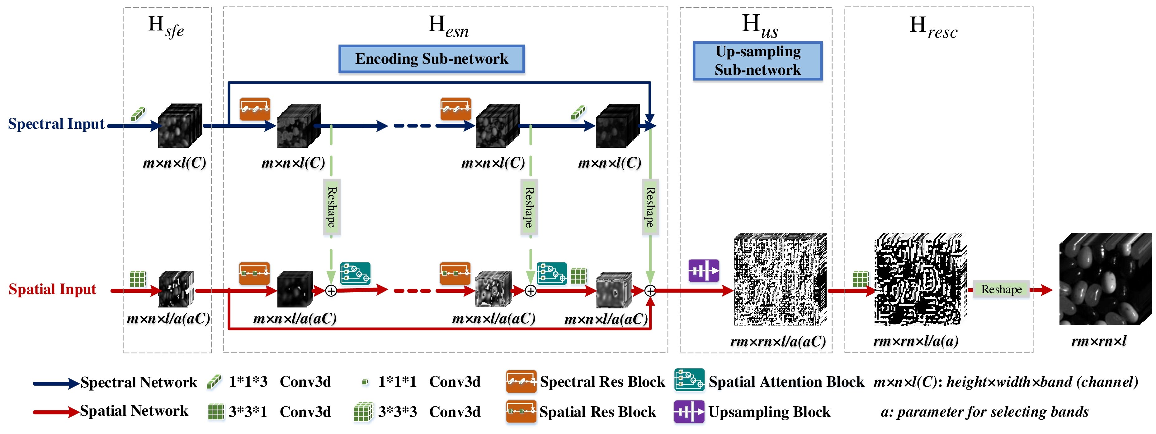
The proposed network is composed of two parts: the 2D stream spatial path and the 1D stream spectral one. In addition, the residual structure and attention mechanism are exploited in our proposed network. Attention blocks are added between the residual blocks in spatial network for taking the relations of non-local regions into account. An illustration is presented in Figure 1. In Figure 1, l is the number of bands, m × n denotes the spatial size of HSI, a is the adjustment parameter to tune the number of bands utilized, C represents the number of feature maps, that is, the number of channels, and r is the up-sampling (down-sampling) factor. It is worth mentioning that in our proposed spatial network, instead of using full bands we select part of bands for spatial enhancement through the a parameter. Due to the fact that some redundant bands may contain similar spatial information, we focus on the effective spatial feature extraction. For instance, if a is set to 2, half of the bands are utilized but more channels are employed for deeper extraction. Both the HSISR and hyperspectral pansharpening can directly employ this network. The only difference between them is the input of the proposed spatial network.
In HSI resolution enhancement procedure, the objective is to estimate a HR super-resolved image from an LR input HSI or an LR input HSI and an HR pan image. Traditionally, 3D convolution is utilized for HSI data, which can extract and encode the spatial–spectral information simultaneously. However, parameter tuning of 3D convolution is heavy. For example, in order to encode a receptive field of , the number of a typical 3D convolution kernel is 27. If we decompose the 3D kernel into a combination of a 1D–2D kernel, such as and , the number of parameters will be reduced to 12. Partially for this reason, kernel decomposing method has become popular in video analysis [21,46].
As illustrated in Figure 1 and Figure 2, our encoding network includes: a 1D convolution path for spectral feature encoding, and a 2D convolution path for spatial features. After the encoding phase, an up-sampling block is proposed to increase the spatial resolution. Here, the transpose convolution or the shuffle pixel convolution could be utilized and achieve similar results. For clear illustration, the hyper-parameters setting of the encoding sub-networks are given in Table 1. The convolution kernel we use is 3 as described in [47], it is said that a stack of small convolution layers has an effective receptive field of larger size convolution. Several articles [47,48,49] have adopted such a design and achieved good results. At present, we can determine the channel and other parameters according to the experimental results and various kinds of structures proposed in the industry [43,47,48,49]. We set channel C = 32 according to our experience and hardware memory limitations. It is worth noting that, actually represents a 1D convolution kernel with the output channel of 32. Generally speaking, we utilize the 1D convolution to extract spectral information, and use 2D convolution for spatial ones. In addition, due to band redundancy and for the sake of reducing computation, we choose different channel and stride for spatial–spectral kernels. As we can see from Table 1, the shapes of the spectral output and spatial output are different. In order to fuse them in an point wise addition manner, we reshape and transpose into , meaning that we pack two bands into the channels of one frame. In this way, we impose the spectral information to the spatial sub-networks in a gradual and hierarchical way.
Supposed that is the input of our network, is the output of our network. is the LR version of its HR counterpart . The HR versions of HSI are available in the training process. For the spatial network, is acquired by applying a Gaussian spatial filter to followed by a down sampling operation with down-sampling (up-sampling) factor r. Generally, the size of with l spectral channels is m × n × l and is of size rm rn × l. For the spatial network, in our proposed architecture, the output of the first convolution layer is:
where represents the first convolution for shallow feature extraction. is also the input of the first residual block.
After the encoding phase, we get :
where means the encoding sub-network containing the residual structure and attention mechanism followed by convolution layers.
Then an up-sampling block is proposed to increase the spatial resolution.
Finally we have the super resolved hyperspectral image:
where denotes the reconstruction layer, which is implemented as one convolution.
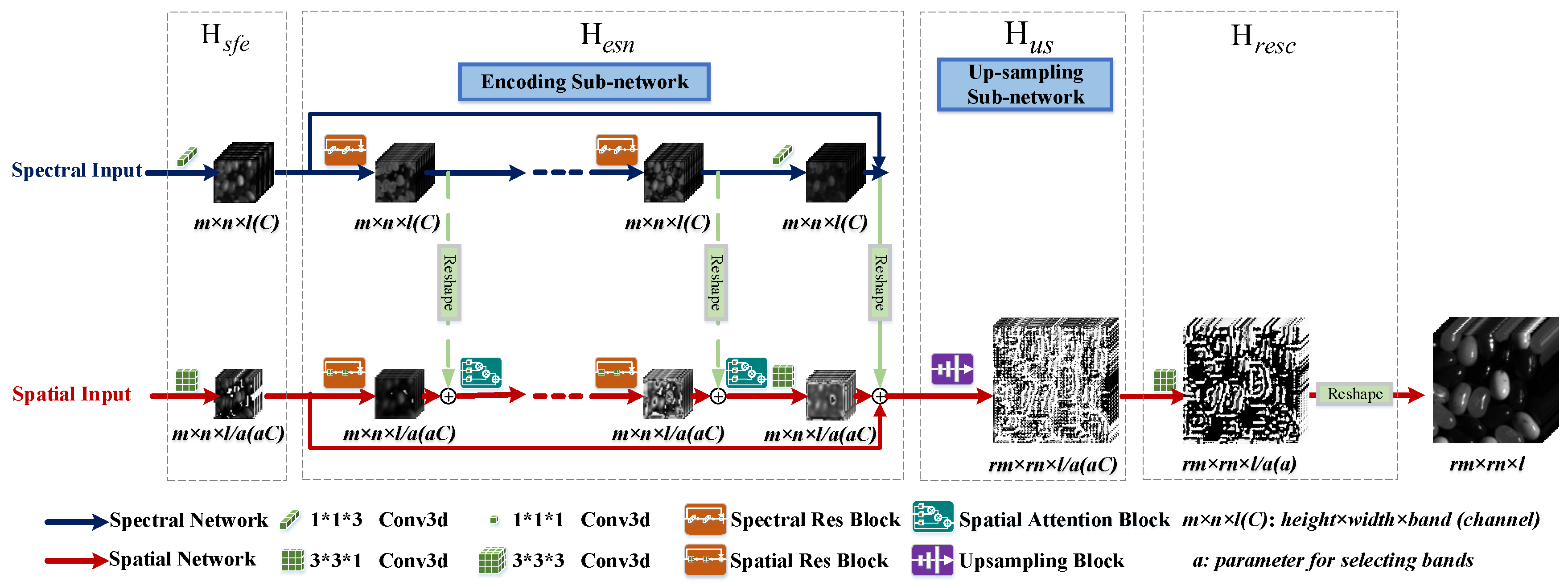
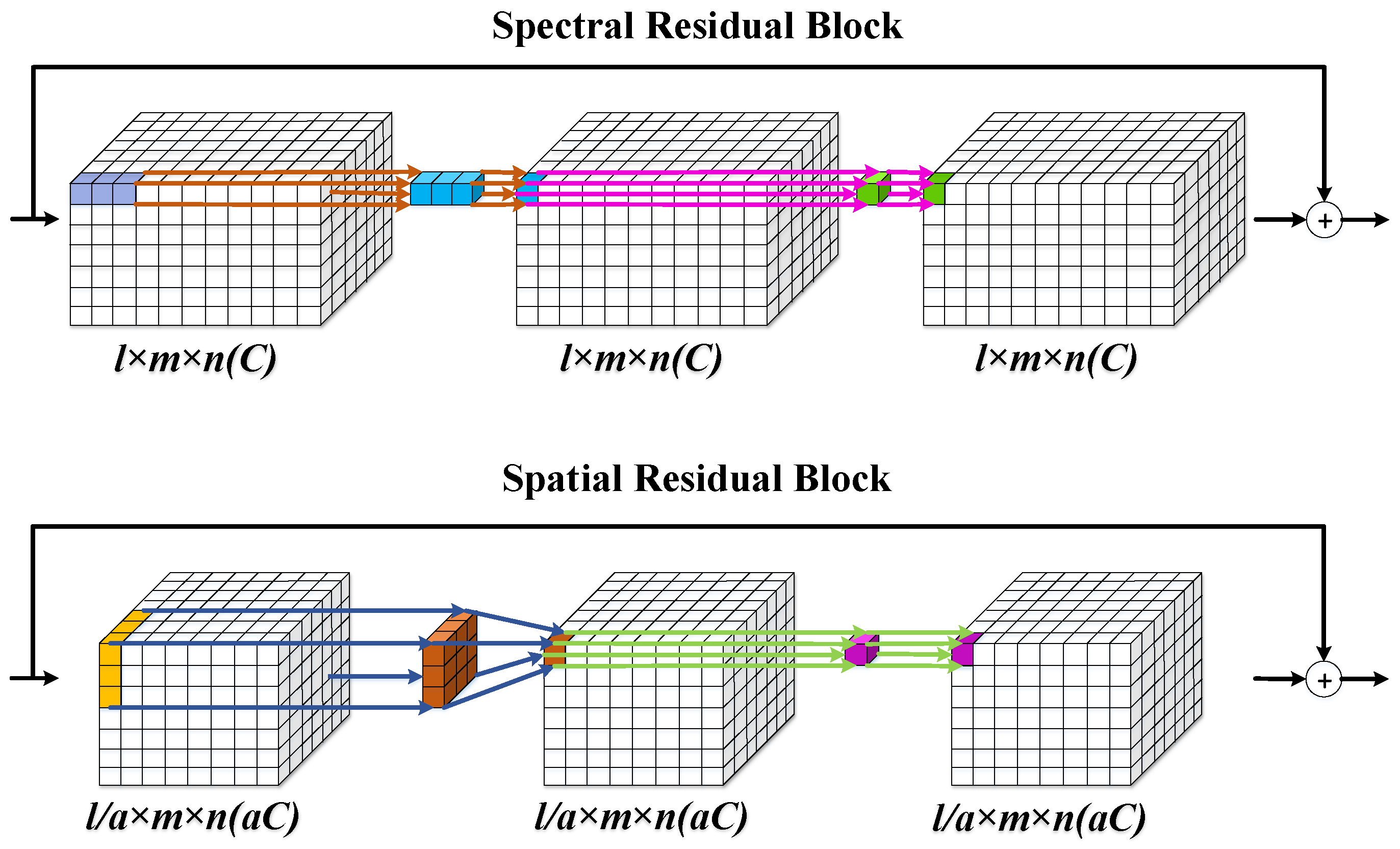
3.2. Residual Structure
The detailed structures of spectral and spatial residual blocks are depicted in Figure 2. It is the visualization of convolution within the residual block. is the input of the first residual block, and is the output of the first residual block. For input , two 3D convolution layers are applied first.
F denotes the current feature maps after two 3D convolutional layers and . The kernel size is , . In fact, the filter has the size of in the spatial network. The setting of other filters in the spatial network are similar to . means Prelu activation function.
At last, F added input to get the output of the band attention residual block.
For the spatial network, except the first residual block, the input of other i-th residual block is the output of -th spatial attention block, then can be calculated as:
For the spectral network, the kernel size is . The has the similar computation process as . The input of other i-th residual block is the output of -th residual block, then can be calculated as:
3.3. Attention Mechanism
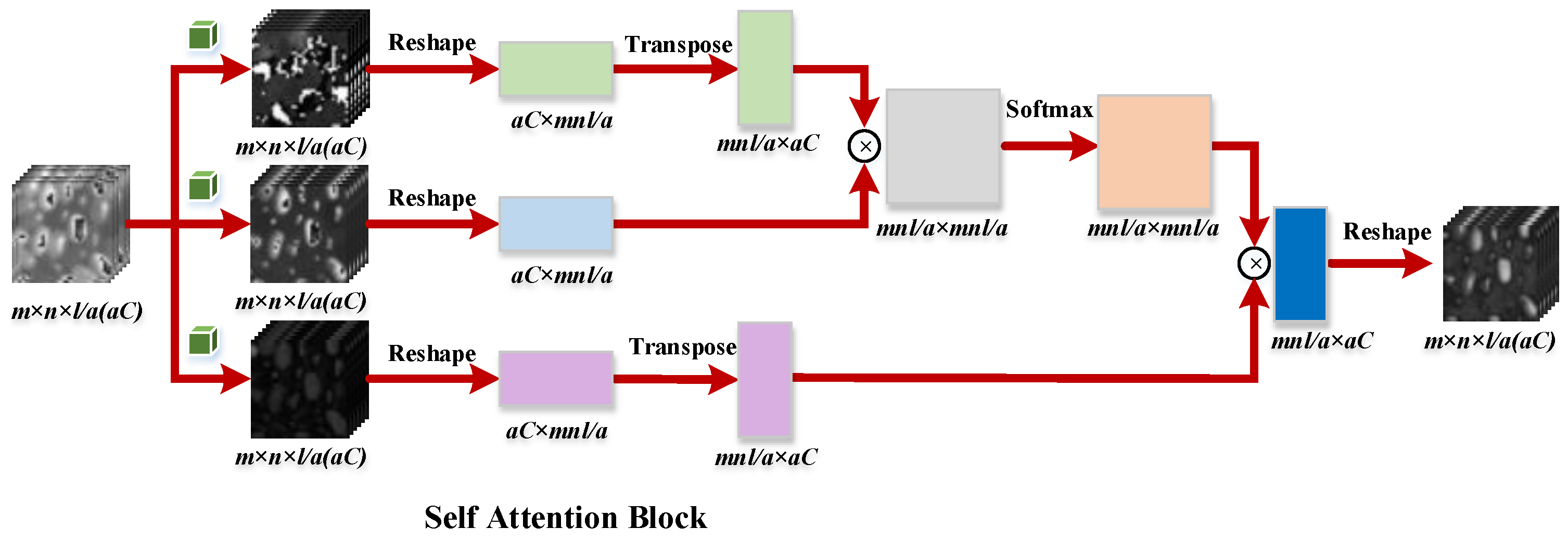
In our proposed architecture, we employ a self attention mechanism in the spatial network for learning non-local region features, which can reference from Figure 3. The attention block is utilized between each residual block. The output features of the i-th spatial residual block are . The output features of the i-th spectral residual block are . Then . Therefore, the input features of the i-th spatial attention block are , which are first transformed into three feature spaces , , , to calculate the attention feature maps, where , and . , and are weight matrix to be learned. In our implementation, a convolution kernel is exploited in spatial domain. Then the attention mask can be calculated through:
where, , . represents the relation between the p-th location and q-th region when synthesizing the p-th region and . Then the output of attention layer can be obtained through:
Consequently, the i-th attention map can be computed through multiplying the output of attention layer by a scale parameter and adding back the input feature maps:
where is initialized as 0. This allows the network to assign the weights to the non-local evidence.
3.4. Pansharpening Case
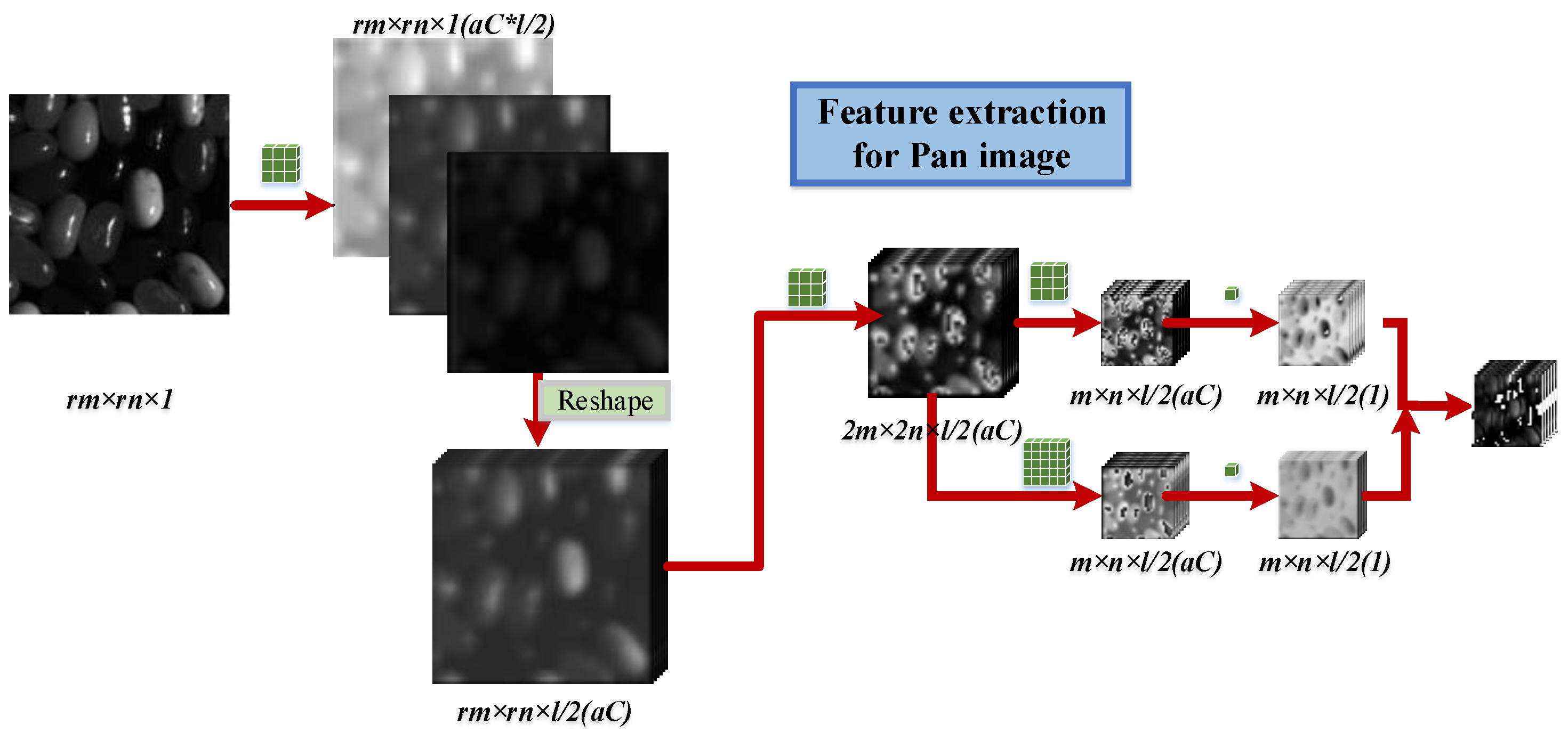
Furthermore, our proposed network can also be used in the task of pansharpening. The input of HSISR are the LR HSIs, and the inputs of hyperspectral pansharpening are LR HSI and pan. When we solve the hyperspectral pansharpening problem, we employ a simple multi-scale CNN to extract the deep spatial features. Different from the input of spatial network in hyperspectral SISR, the input of spatial network becomes in hyperspectral pansharpening and the following operations are in line with the hyperspectral SISR. The detailed network and parameters setting for extraction of the deep features can be referenced from Figure 4 and Table 2. Generally speaking, the pan image can be transformed into LR HSI through a series of pooling. In convolution neural networks, a convolution layer with a step size of 2 can replace the pooling layer. The performance is basically consistent, or even slightly better [49].
Let be the input of the spatial inputs of hyperspectral pansharpening block, and be the output of the spatial inputs of hyperspectral pansharpening block.
For input , one 3D convolution layers are applied first.
denote the current feature maps after 3D convolutional layers . is the Prelu activation function.
The data of spatial dimension is converted to the band dimension by a reshape operation.
where .
Then, 3D convolution layers are applied:
denote the current feature maps after 3D convolutional layers .
Multi-scale feature exaction is represented as follows:
At last, we get by concating and :
3.5. Loss Function
In our proposed 1D–2D attentional CNN, only norm loss and spectral loss are utilized to guide the training process:
Given the ground truth and the super-resolved image , these two loss functions are designed as
where l, m, n and r denote the spectral bands, height, width and the up-sampling(down-sampling) factor, respectively, denotes the norm of vector, denotes the spectral vector at the i-th row and j-th column in HR HSI that is the referenced ground truth, and is the reconstructed spectral vector with the same spatial position after SR. In our experiments, is set to 0.01.
4. Experiments Setting
In this section, we conduct a series of experiments on four typical hyperspectral sets to evaluate the performance of our proposed network. As the performance of deep learning-based algorithms is better than the traditional algorithm, three state-of-the-art deep learning methods with public codes are selected as the baseline for comparison purposes in hyperspectral SISR: LapSRN [50], 3DFCNN [40] and GDRRN [43]. Three classic hyperspectral pansharpening algorithms are also selected for comparison, such as the GFPCA [17], the CNMF [22], and the Hysure [14].
4.1. Evaluation Criteria
To comprehensively evaluate the performance of the proposed methods, several classical evaluation metrics are utilized: mean peak signal-to noise ratio (MPSNR), mean structural similarity index (MSSIM), mean root mean square error (MRMSE), spectral angle mapper (SAM), the cross correlation (CC), and the erreur relative global adimensionnelle de synthese (ERGAS).
The MPSNR and MRMSE can estimate the similarity between the generated image and the ground truth image through the mean squared error. The MSSIM emphasizes the structural consistency with the ground truth image. The SAM is utilized to evaluate the spectral reconstruction quality of each spectrum at pixel-levels, which calculates the average angle between spectral vectors of the generated HSI and the ground truth one. The CC reflects the geometric distortion, and the ERGAS is a global indicator of the fused image quality [51]. The ideal values of the MPSNR, MSSIM and CC are 1. As for the SAM, RMSE, and ERGAS, the optimal values are 0.
Given a reconstruction image and a ground truth image S, these four evaluation metrics are defined as:
where is the maximum intensity in the k-th band, and are the mean values of and respectively, and are the variance of and respectively, is the covariance between and , and are two constants used to improve stability, is the number of pixels, denotes the dot product of two spectra and , represents norm operation, and d denotes the ratio between the pixel size of the PAN image and the HSI.
In these evaluation metrics, the larger the MPSNR, MSSIM, and CC, the more similar the reconstructed HSI and the ground truth one. Meanwhile, the smaller the SAM, MRMSE, and ERGAS, the more similar the reconstructed and the ground truth ones.
4.2. Datasets and Parameter Setting
Pavia University and Pavia Center are two hyperspectral scenes acquired via the ROSIS sensor, which covers 115 spectral bands from 0.43 to 0.86 m, which are employed in our experiments for hyperspetral SISR comparison. The geometric resolution is 1.3 m. The University of Pavia image has 610 × 340 pixels, each having 103 bands after bad-band and noisy band removal. The Pavia Center scene contains 1096 × 1096 pixels, 102 spectral bands left after bad-band removal. In the Pavia center scene, only 1096 × 715 valid pixels are utilized after discarding the samples with no information in this experiment. For each dataset, a 144 × 144 sub-region is selected to evaluate the performance of our proposed 1D–2D attentional CNN, another 144 × 144 sub-region is selected for verication, while the remaining are used for training.
The CAVE dataset and Harvard dataset are two publicly available hyperspectral datasets for hyperspectral pansharpening comparison. The CAVE dataset includes 32 HSIs of real-world materials and objects captured in the laboratory environment. All the HSIs in the CAVE dataset have 31 spectral bands ranging from 400 nm to 700 nm at 10 nm spectral resolution, and each band has a spatial dimension of pixels. The Harvard dataset comprises 50 HSIs of indoor and outdoor scenes such as offices, streetscapes, and parks under daylight illumination. Each HSI has a spatial resolution of with 31 spectral bands covering the spectrum range from 420 nm to 720 nm at steps of 10 nm. For CAVE dataset, we select the first 16 images as the training dataset, four images as the validation dataset, and the remaining 12 images are utilized as the testing dataset. For the Harvard dataset, we employ 26 HSIs for training, six HSIs for verification and the remaining 18 for testing. The simulated PAN images with the same spatial size as the original HSIs are generated by averaging the spectral bands of the visible range of the original HSIs.
The proposed 1D–2D attentional framework is implemented on the deep learning framework named Pytorch. Training was performed on an NVIDIA GTX1080Ti GPU. The parameters of the network were optimized using Adam modification and the initial learning rate is set to . We try the learning rate set . The experimental results show that when the initial learning rate is 0.001, we get the best results compared to other learning rates.
5. Experimental Results and Discussions
In this section, we evaluate our proposed algorithm from the quantitative and qualitative analysis on both HSISR and hyperspectral pansharpening results. For adaptive different SR tasks, a is set to 2 in our experiments. It is worth noting that all the algorithms are under same condition of the experimental setting, which indicates that both the comparison algorithms and the proposed algorithm are well-trained through employing same training samples. Furthermore, through the aforementioned introduction of data sets, the test data is not included in the training data.
5.1. Discussion on the Proposed Framework: Ablation Study
In this section, we first evaluate the efficiency of our proposed architecture taking the Pavia Center dataset as a example. Our proposed approach contains two parallel architectures: 2D stream spatial residual CNN and 1D stream spectral residual CNN. Traditionally, 3D convolutional kernels are utilized for extracting and encoding the spatial–spectral information simultaneously with heavy parameters tuning. Here we use a 1D () and a 2D () convolutions for learning spatial–spectral features respectively but with similar or even better results. To demonstrate our effectiveness of 1D–2D convolutional kernels, we conduct a set of experiments on the Pavia Center dataset. Spa denotes only a 2D stream spatial network in our proposed algorithm is employed for evaluation. Spe denotes that only a 1D stream spectral network is utilized. The 3D conv indicates using a 3D convolutional kernel to extract spatial–spectral information simultaneously but with the same number of layers as our proposed algorithm. The spe-spa denotes our proposed algorithm without using spatial attention. The number of channels utilized are depicted following the algorithms’ name. For instance, the numbers of channels in the Spe-spa network are set to (32,32), which means the channels of the spatial network are set to 32 (with full bands). Meanwhile, the channels of the spectral network are set to 32. For evaluation our proposed parallel framework, the channels are set to 32 for all the compared methods.
From Table 3, we can see that when using only the spatial or spectral network, the four criteria cannot reach satisfying values simultaneously. For instance, the MRMSE and MPSNR obtained via the spectral network is smaller than with the Spe-spa network, which indicates that the spatial information cannot be well extracted and encoded. The SAM achieved only by the spatial network is larger than other networks, as the inadequate spectral information is learned while suppressing the spectral fidelity. Furthermore, our proposed algorithm offers the best resolution enhancement result compared to the Spe-spa network implying that our spatial attention mechanism can take a positive role in the resolution enhancement problem. In addition, we tabulate the kernels, channels, and strides used in comparison experiments. The total number of parameters utilized in each network are also listed in each network learning. From Table 4, it can be concluded that the design of parallel architecture does reduce the number of parameters and has a low computational complexity.
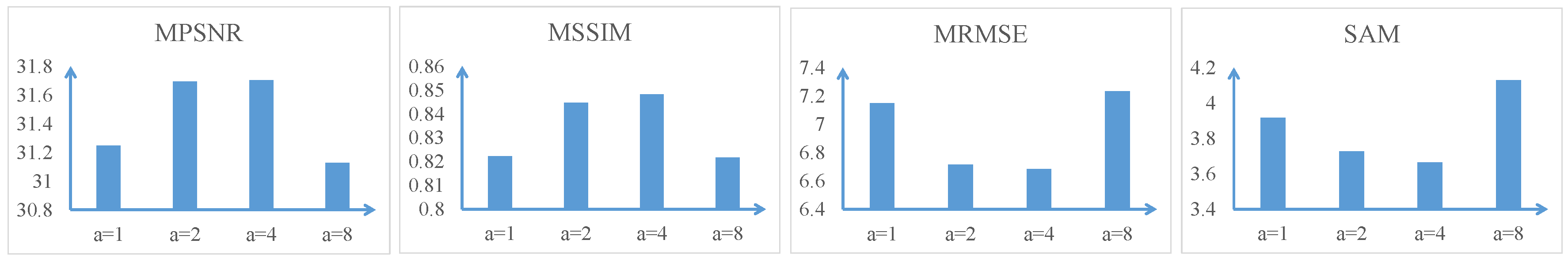
Our 1D–2D attentional convolutional neural network employs a separation strategy to extract the spatial–spectral information and then fuse them gradually. Specifically, a a 1D convolution path is used for spectral feature encoding, and a 2D convolution path is used for the spatial features. In fact, the spectral bands of HSI are highly redundant, so, we do not need to utilize full bands of HSIs. Dimensionality reduction is an effective preprocessing step to discard the redundant information [52,53,54]. Therefore, instead of using full bands we select part of the bands for spatial enhancement through the a parameter. Furthermore, the emphasis of the spatial network is to extract and enhance the spatial features. The less bands we select, the more filters are used, and the network can learn more sufficient and deeper spatial information. Additionally, this method can ensure that the shape of the spectral path is the same as the spatial path after the reshape operation, and can integrate the information of the two branches through hierarchical side connections. We evaluate our proposed network through a factors such as 1, 2, 4, and 8. From Figure 5, we can see that with the increasing number of a, the performance of our proposed algorithm based on the Pavia Center dataset increases first and then decreases. When a is equal to 4, the SR results have the best performance. Specifically, when a is equal to 1, all bands are utilized and the spectral bands of HSI are highly redundant. If a is equal to 2 or 4, then half of the bands or a 1/4 of the bands are utilized, but more channels are employed for deeper extraction. All of them can achieve better results. If a is equal to 8, then 1/8 of the bands are utilized. There is a greater possibility that information loss is severe, resulting in a poor performance result. This is because when a is too small, the spectral information is redundant and when a is too large, the information loss is serious. Then, the performance decreases. Therefore, there exists a trade-off between redundant information and information loss. Experiments show that when a is equal to 4, the SR results has the best performance on Pavia Center dataset.
In this section, we evaluate our proposed algorithm from the quantitative and qualitative analysis on both HSISR and hyperspectral pansharpening results. For adaptive different SR tasks, a is set to 2 in our experiments.
5.1.1. Results of Hyperspectral SISR and Analysis
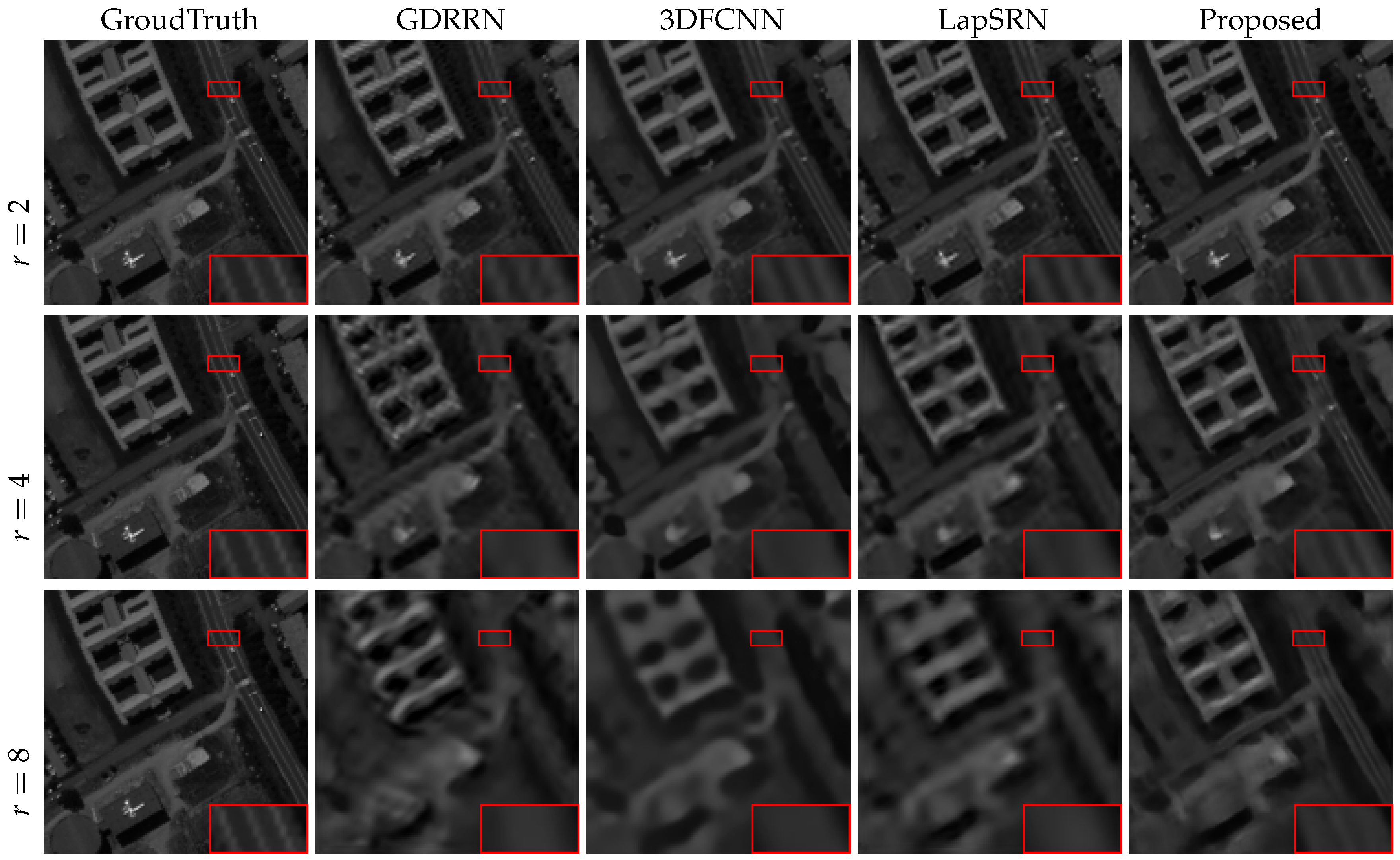
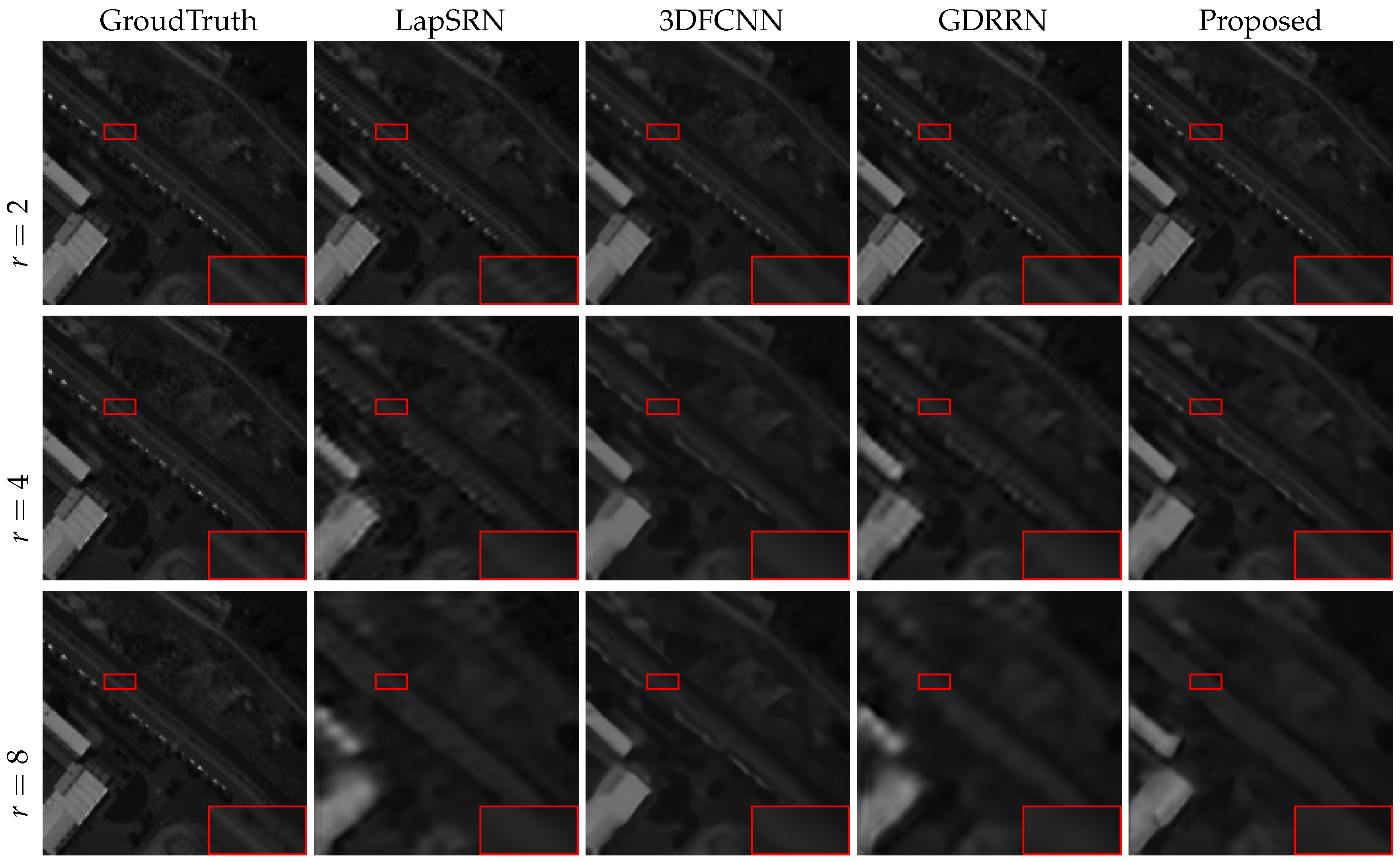
We evaluate our proposed network through different up-sampling factors such as 2, 4, and 8. Table 5 and Table 6 tabulate the quantitative results under different up-sampling factors. Their corresponding visual results are depicted in Figure 6 and Figure 7. The Pavia University dataset is displayed in band 49. The Pavia Center dataset is displayed in band 13.
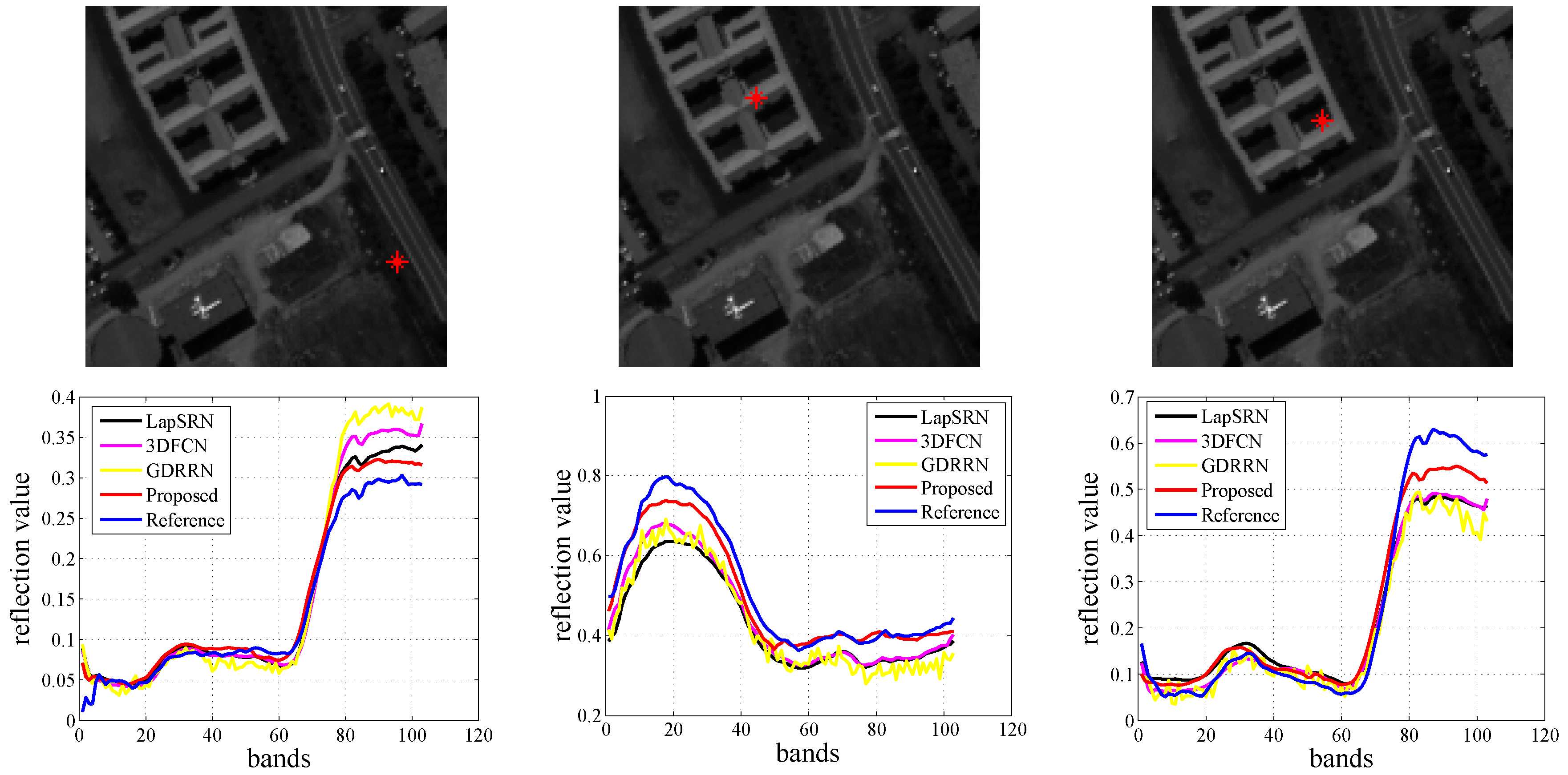
Our proposed method outperforms other comparison algorithms with different up-sampling factors. Despite the difficulty of HSISR at a large up-sampling factor, our 8x model still performed well. For the results achieved from the Pavia University dataset, it is observed that: (1) The proposed method significantly outperforms with the highest MPSNR, MSSIM, and lowest MRMSE and SAM values for all the cases; (2) Compared with the GDRRN, the improvements of our methods are 2.1276 dB and 0.0672 in terms of MPSNR and MSSIM, meanwhile the decreases are 1.7729 and 1.4089 in terms of MRMSE and SAM through averaging the values under different up-sampling factor; (3) The proposed method achieves the best spatial reconstruction compared to other SR methods irrelevant to the up-sampling factor. It can also be clearly seen from Figure 6 that the image reconstructed by the proposed method has finer texture details than the other comparison methods, especially, when under 8x up-sampling factor, the texture and edge information of the region in the red rectangle is clearer than the other methods; (4) The proposed method achieves the best spectral fidelity with the lowest SAM in all the cases. Figure 8 further demonstrates the spectrum after hyperspectral resolution enhancement. It is implied that the spectra reconstructed by the proposed algorithm is the closest to its ground-truth than those achieved by comparison methods.
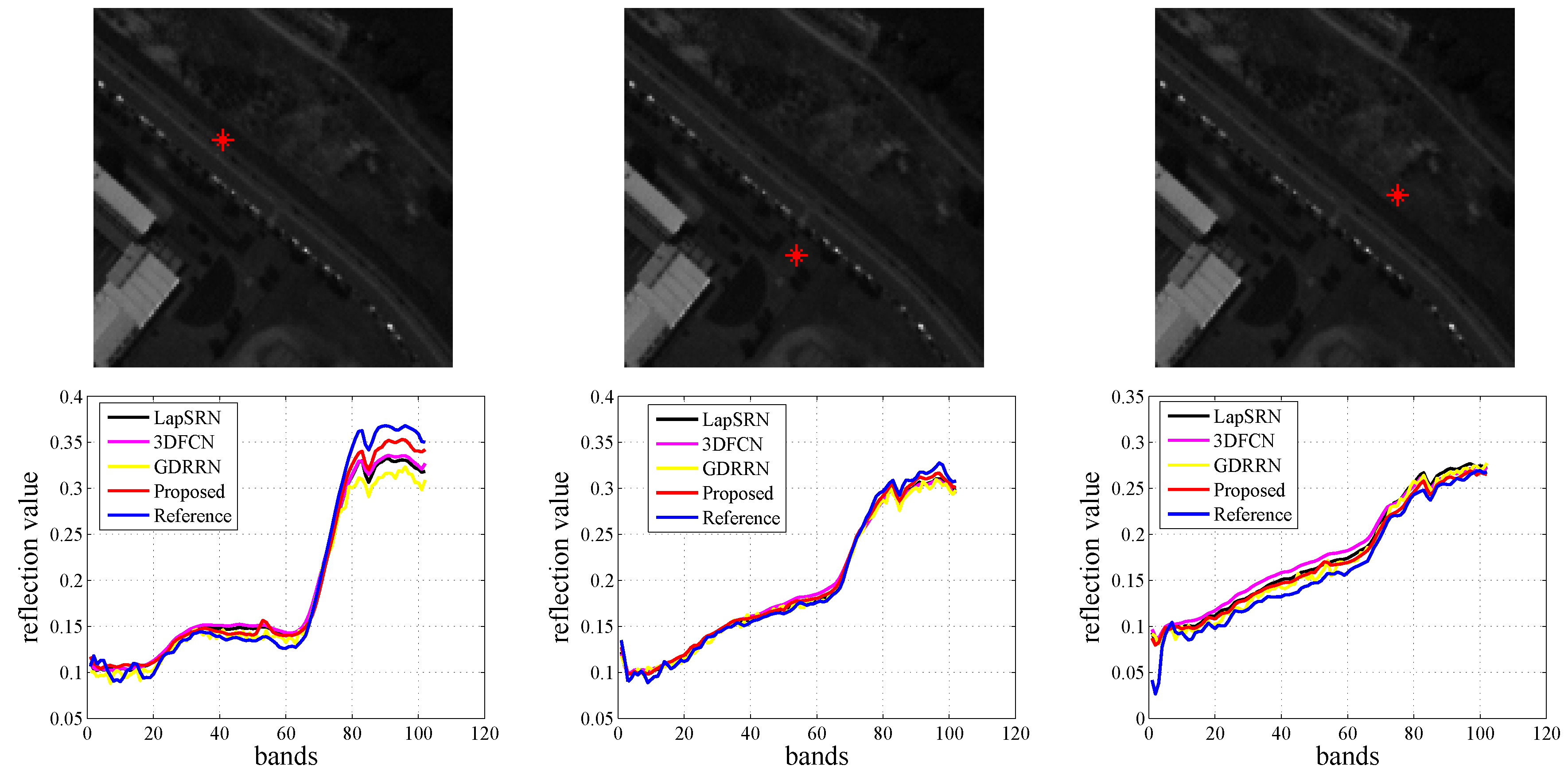
From the results obtained from the Pavia Center dataset in Figure 7 and Table 6, we can see that, compared with other methods, our proposed method still has superior SR results. For instance, compared with the GDRRN, MPSNR increased by an average of 2.2042, MSSIM improved by 0.0457, MRMSE decreased by 1.4783, and SAM dropped by 0.9212. Furthermore, Figure 9 depicts the spectral accuracy achieved via different HSISR methods, and it indicates that our proposed method can reconstruct more similar spectra than other methods. Therefore, the results on the Pavia Center dataset have similar phenomena as the results on the Pavia University dataset.
From the results presented above, the values of MPSNR, MSSIM, MRMSE and SAM metrics achieved by our proposed algorithm are preferable than other methods implying that the proposed algorithm can learn and enhance the spatial features more reasonable with consistency of the structure features when considering non-local spatial information through the spatial attention mechanism. Furthermore, the spectral fidelity of algorithm is kept most accurate due to the fact that a separate spectral residual network is used specifically for maintaining spectral information. Therefore, it can be concluded that the proposed algorithm outperforms on these two datasets acquired by the ROSIS sensor.
5.1.2. Results of Hyperspectral Pansharpening and Analysis
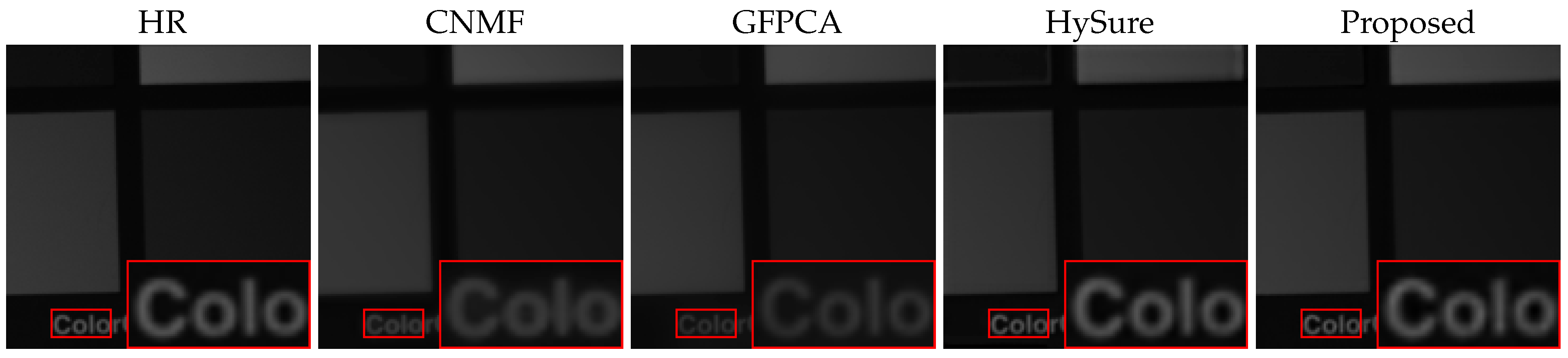
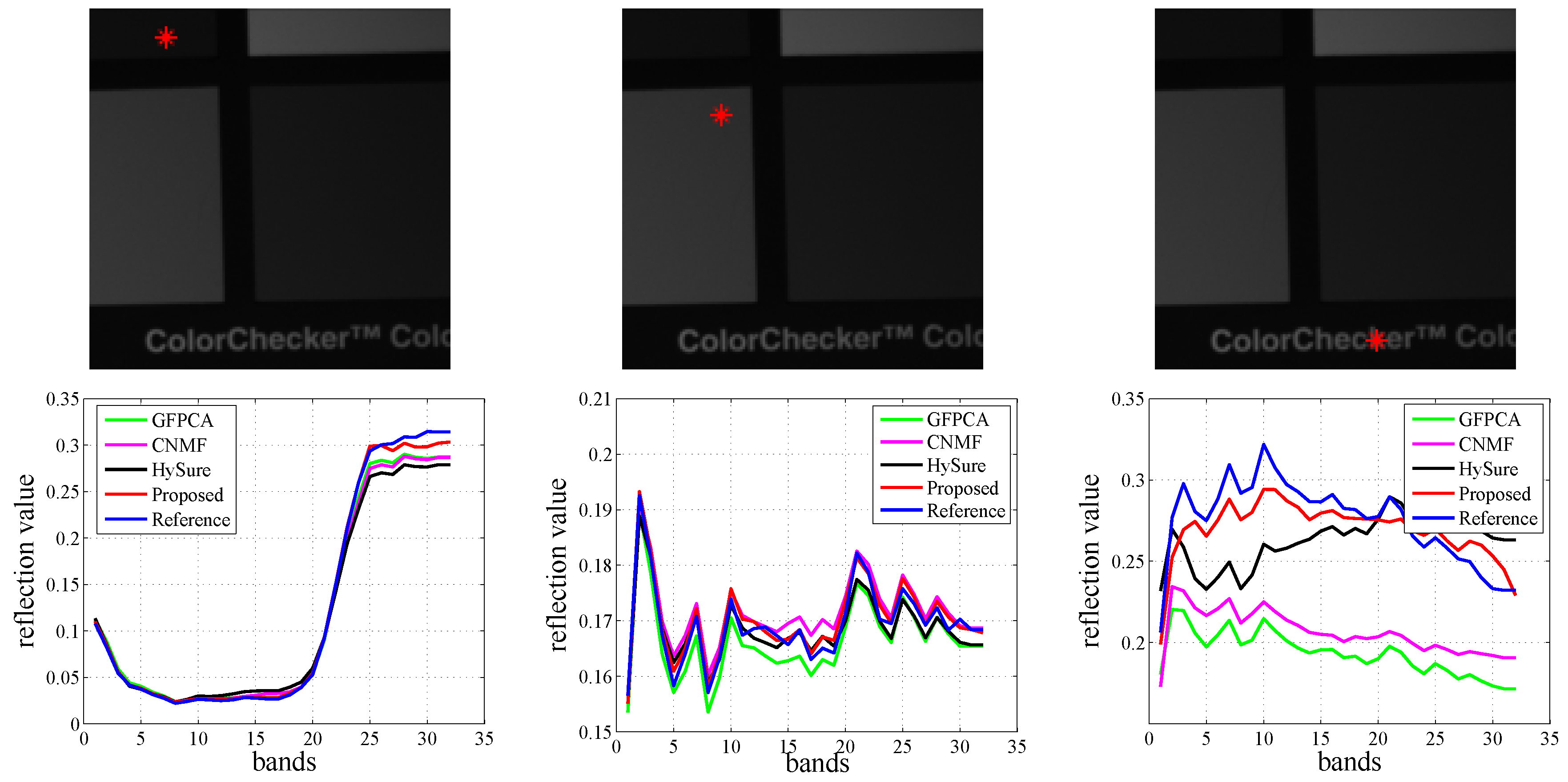
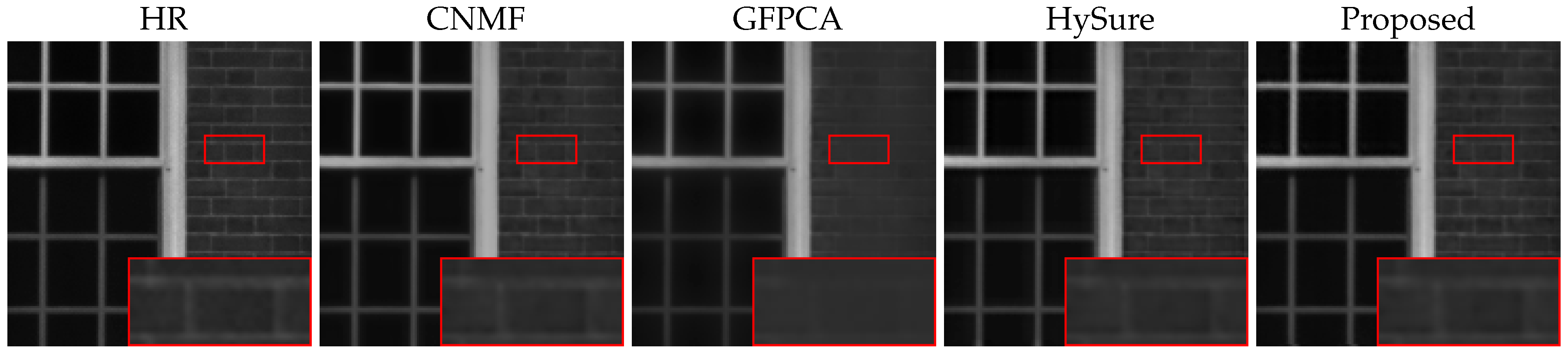
We also evaluate our proposed network in hyperspectral pansharpening when the up-sampling factor is set as 4. Table 7 tabulates the quantitative results of different hyperspectral pansharpening methods based on the Cave dataset. It can be seen that our proposed method achieved the best performance in terms of ERGAS, CC, MRMSE, and SAM. Both SAM and ERGAS are far smaller than the other comparison algorithms. Compared with the GFPCA algorithm, CC increased by 0.0161, ERGAS decreased by 2.1487, MRMSE reduced by 0.0099, and SAM dropped by 1.443. Indicating that the proposed resolution enhancement algorithm can not only extract better spatial information but also better refrains the spectral distortion. Figure 10 and Figure 11 demonstrate the visual results and spectrum of the super-resolved HSI respectively, from which we can acknowledge that the texture and edge features obtained by our proposed algorithm are the clearest and most accurate. The CAVE dataset is displayed in band 28, and the Harvard dataset is displayed in band 18.
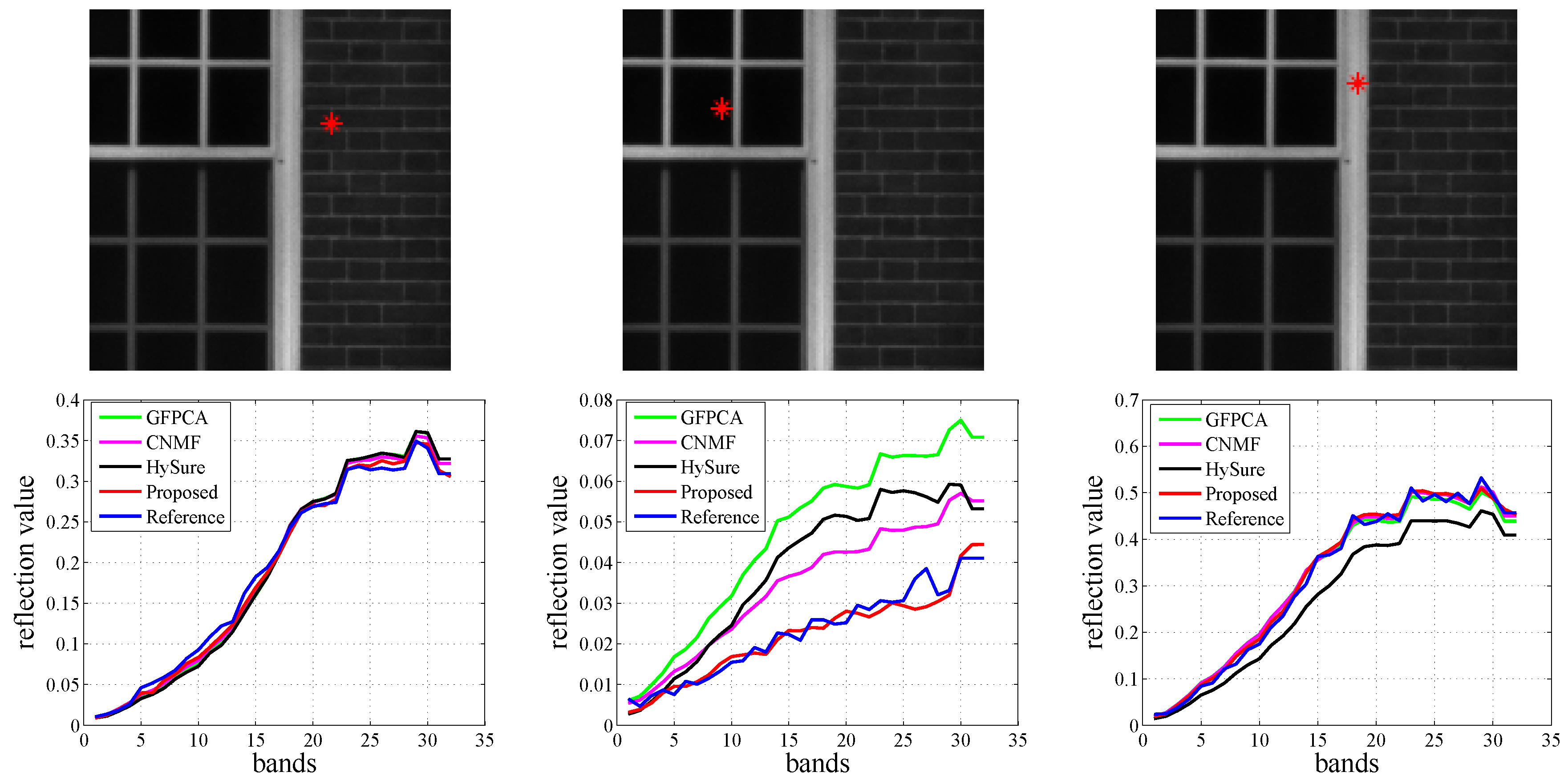
In addition, we design a set of experiments on the Harvard dataset. Table 8 tabulates the quantitative results of different hyperspectral pansharpening methods based on the Harvard dataset. Furthermore, our proposed algorithm has the best fusion performance compared to the other comparison algorithms. In specific, the ERGAS obtained via our method is the smallest, which means that our 1D–2D attentional CNN can obtain the best fusion performance. Also, the displays from Figure 12 and Figure 13 further demonstrate the superiority and advantage of our proposed algorithm for spatial resolution enhancement and spectral reconstruction.
Based on HSISR and hyperspectral pansharpening, our model can provide a performance superior to other state-of-the-art methods.
6. Conclusions
In this paper, a novel attention based 1D–2D spatial–spectral CNN with parallel architecture is proposed for the HSI resolution enhancement problem. It can be used not only for hyperspectral SISR, but also for HSI pansharpening. Our method consists of a 1D stream spectral network and a 2D stream spatial network with and kernels respectively. The spatial network focuses on improving the spatial resolution through exploiting the self attention mechanism; meanwhile the spectral network concentrates on the spectral fidelity. Furthermore, the hierarchical side connection is adopted for fusing the spatial–spectral features and the correction of distortion of partial edge pixels. From the experimental results, the proposed algorithm is very efficient, and achieves significant improvement compared with other state-of-the-art methods in the field of resolution enhancement of HSIs.
Author Contributions
J.L. and Q.D. conceived and designed the study; R.C. performed the experiments; R.S. shared part of the experiment data; R.S and B.L. analyzed the data; J.L. and B.L. wrote the paper. Y.L. and Q.D. reviewed and edited the manuscript. All authors read and approved the manuscript.
Acknowledgments
This work was supported in part by the National Nature Science Foundation of China (no. 61901343), the China Postdoctoral Science Foundation (no. 2017M623124) and the China Postdoctoral Science Special Foundation (no. 2018T111019). The project was also partially supported by the Open Research Fund of CAS Key Laboratory of Spectral Imaging Technology (no. LSIT201924W) and the Fundamental Research Funds for the Central Universities JB190107. It was also partially supported by the National Nature Science Foundation of China (nos. 61571345, 61671383, 91538101, 61501346 and 61502367), the 111 project (B08038), and the Innovation Fund of Xidian University (no. 10221150004).
Conflicts of Interest
The authors declare that we have no financial and personal relationships with other people or organizations that can inappropriately influence our work and that this paper was not published before, the founding sponsors had no role in the design of the study; in the collection, analyses, or interpretation of data; in the writing of the manuscript, and in the decision to publish the results.
References
- Akgun, T.; Altunbasak, Y.; Mersereau, R.M. Super-resolution reconstruction of hyperspectral images. IEEE Trans. Image Process. 2005, 14, 1860–1875. [Google Scholar] [CrossRef] [PubMed]
- Andrews, H.C.; Patterson, C.L. Digital Interpolation of Discrete Images. IEEE Trans. Comput. 1976, 25, 196–202. [Google Scholar] [CrossRef]
- Shima, T. Bumpless monotonic bicubic interpolation for MOSFET device modelling. IEE Proc. I Solid State Electron. Devices 1985, 132, 147–150. [Google Scholar] [CrossRef]
- Patel, R.C.; Joshi, M.V. Super-Resolution of Hyperspectral Images: Use of Optimum Wavelet Filter Coefficients and Sparsity Regularization. IEEE Trans. Geosci. Remote Sens. 2015, 53, 1728–1736. [Google Scholar] [CrossRef]
- Wang, Y.; Chen, X.; Han, Z.; He, S. Hyperspectral Image Super-Resolution via Nonlocal Low-Rank Tensor Approximation and Total Variation Regularization. Remote Sens. 2017, 9, 1286. [Google Scholar] [CrossRef]
- Rong, K.; Jiao, L.; Wang, S.; Liu, F. Pansharpening Based on Low-Rank and Sparse Decomposition. IEEE J. Sel. Top. Appl. Earth Obs. Remote Sens. 2014, 7, 4793–4805. [Google Scholar] [CrossRef]
- Tu, T.M.; Su, S.C.; Shyu, H.C.; Huang, P.S. A new look at IHS-like image fusion methods. Inf. Fusion 2001, 2, 177–186. [Google Scholar] [CrossRef]
- Aiazzi, B.; Baronti, S.; Selva, M. Improving Component Substitution Pansharpening Through Multivariate Regression of MS+Pan Data. IEEE Trans. Geosci. Remote Sens. 2007, 45, 3230–3239. [Google Scholar] [CrossRef]
- Liu, J. Smoothing filter-based intensity modulation: A spectral preserve image fusion technique for improving spatial details. Int. J. Remote Sens. 2000, 21, 3461–3472. [Google Scholar] [CrossRef]
- Aiazzi, B.; Alparone, L.; Baronti, S.; Garzelli, A.; Selva, M. MTF-tailored multiscale fusion of high-resolution MS and Pan imagery. Photogramm. Eng. Remote Sens. 2006, 72, 591–596. [Google Scholar] [CrossRef]
- Vivone, G.; Restaino, R.; Dalla Mura, M.; Licciardi, G.; Chanussot, J. Contrast and error-based fusion schemes for multispectral image pansharpening. IEEE Geosci. Remote Sens. Lett. 2014, 11, 930–934. [Google Scholar] [CrossRef]
- Shensa, M.J. The discrete wavelet transform: Wedding the a trous and Mallat algorithms. IEEE Trans. Signal Process. 1992, 40, 2464–2482. [Google Scholar] [CrossRef]
- Wei, Q.; Bioucas-Dias, J.; Dobigeon, N.; Tourneret, J. Hyperspectral and Multispectral Image Fusion Based on a Sparse Representation. IEEE Trans. Geosci. Remote Sens. 2015, 53, 3658–3668. [Google Scholar] [CrossRef]
- Simões, M.; Bioucas-Dias, J.; Almeida, L.B.; Chanussot, J. A Convex Formulation for Hyperspectral Image Superresolution via Subspace-Based Regularization. IEEE Trans. Geosci. Remote Sens. 2015, 53, 3373–3388. [Google Scholar] [CrossRef]
- Wei, Q.; Dobigeon, N.; Tourneret, J.Y. Fast fusion of multi-band images based on solving a Sylvester equation. IEEE Trans. Image Process. 2015, 24, 4109–4121. [Google Scholar] [CrossRef]
- Hoyer, P.O. Non-negative sparse coding. In Proceedings of the 12th IEEE Workshop on Neural Networks for Signal Processing, Martigny, Switzerland, 6 September 2002; pp. 557–565. [Google Scholar] [CrossRef]
- Liao, W.; Huang, X.; Van Coillie, F.; Gautama, S.; Pižurica, A.; Philips, W.; Liu, H.; Zhu, T.; Shimoni, M.; Moser, G.; et al. Processing of Multiresolution Thermal Hyperspectral and Digital Color Data: Outcome of the 2014 IEEE GRSS Data Fusion Contest. IEEE J. Sel. Top. Appl. Earth Obs. Remote Sens. 2015, 8, 2984–2996. [Google Scholar] [CrossRef]
- Dong, W.; Xiao, S.; Xue, X.; Qu, J. An Improved Hyperspectral Pansharpening Algorithm Based on Optimized Injection Model. IEEE Access 2019, 7, 16718–16729. [Google Scholar] [CrossRef]
- Li, Y.; Qu, J.; Dong, W.; Zheng, Y. Hyperspectral pansharpening via improved PCA approach and optimal weighted fusion strategy. Neurocomputing 2018, 315, 371–380. [Google Scholar] [CrossRef]
- Wang, X.; Girshick, R.; Gupta, A.; He, K. Non-local neural networks. In Proceedings of the IEEE Conference on Computer Vision and Pattern Recognition, Salt Lake City, UT, USA, 18–22 June 2018; pp. 7794–7803. [Google Scholar]
- Feichtenhofer, C.; Fan, H.; Malik, J.; He, K. SlowFast Networks for Video Recognition. arXiv 2018, arXiv:1812.03982. [Google Scholar]
- Yokoya, N.; Yairi, T.; Iwasaki, A. Coupled nonnegative matrix factorization unmixing for hyperspectral and multispectral data fusion. IEEE Trans. Geosci. Remote Sens. 2012, 50, 528–537. [Google Scholar] [CrossRef]
- Li, J.; Yuan, Q.; Shen, H.; Meng, X.; Zhang, L. Hyperspectral Image Super-Resolution by Spectral Mixture Analysis and Spatial–Spectral Group Sparsity. IEEE Geosci. Remote Sens. Lett. 2016, 13, 1250–1254. [Google Scholar] [CrossRef]
- Xu, X.; Tong, X.; Li, J.; Xie, H.; Zhong, Y.; Zhang, L.; Song, D. Hyperspectral image super resolution reconstruction with a joint spectral-spatial sub-pixel mapping model. In Proceedings of the 2016 IEEE International Geoscience and Remote Sensing Symposium (IGARSS), Beijing, China, 10–15 July 2016; pp. 6129–6132. [Google Scholar]
- Pan, Z.; Yu, J.; Huang, H.; Hu, S.; Zhang, A.; Ma, H.; Sun, W. Super-Resolution Based on Compressive Sensing and Structural Self-Similarity for Remote Sensing Images. IEEE Trans. Geosci. Remote Sens. 2013, 51, 4864–4876. [Google Scholar] [CrossRef]
- Li, J.; Du, Q.; Li, Y.; Li, W. Hyperspectral Image Classification With Imbalanced Data Based on Orthogonal Complement Subspace Projection. IEEE Trans. Geosci. Remote Sens. 2018, 56, 3838–3851. [Google Scholar] [CrossRef]
- Tian, C.; Xu, Y.; Fei, L.; Yan, K. Deep Learning for Image Denoising: A Survey. arXiv 2018, arXiv:1810.05052. [Google Scholar]
- Li, Y.; Zheng, W.; Cui, Z.; Zhang, T. Face recognition based on recurrent regression neural network. Neurocomputing 2018, 297, 50–58. [Google Scholar] [CrossRef]
- Li, B.; Dai, Y.; He, M. Monocular depth estimation with hierarchical fusion of dilated CNNs and soft-weighted-sum inference. Pattern Recognit. 2018, 83, 328–339. [Google Scholar] [CrossRef]
- Li, B.; Shen, C.; Dai, Y.; van den Hengel, A.; He, M. Depth and surface normal estimation from monocular images using regression on deep features and hierarchical CRFs. In Proceedings of the CVPR, Boston, MA, USA, 8–10 June 2015; pp. 1119–1127. [Google Scholar]
- Zhong, P.; Gong, Z.; Li, S.; Schönlieb, C. Learning to Diversify Deep Belief Networks for Hyperspectral Image Classification. IEEE Trans. Geosci. Remote Sens. 2017, 55, 3516–3530. [Google Scholar] [CrossRef]
- Li, W.; Wu, G.; Zhang, F.; Du, Q. Hyperspectral Image Classification Using Deep Pixel-Pair Features. IEEE Trans. Geosci. Remote Sens. 2017, 55, 844–853. [Google Scholar] [CrossRef]
- Li, J.; Xi, B.; Li, Y.; Du, Q.; Wang, K. Hyperspectral Classification Based on Texture Feature Enhancement and Deep Belief Networks. Remote Sens. 2018, 10, 396. [Google Scholar] [CrossRef]
- Chen, Y.; Zhao, X.; Jia, X. Spectral–Spatial Classification of Hyperspectral Data Based on Deep Belief Network. IEEE J. Sel. Top. Appl. Earth Obs. Remote Sens. 2015, 8, 2381–2392. [Google Scholar] [CrossRef]
- Li, J.; Zhao, X.; Li, Y.; Du, Q.; Xi, B.; Hu, J. Classification of Hyperspectral Imagery Using a New Fully Convolutional Neural Network. IEEE Geosci. Remote Sens. Lett. 2018, 15, 292–296. [Google Scholar] [CrossRef]
- Chen, Y.; Jiang, H.; Li, C.; Jia, X.; Ghamisi, P. Deep Feature Extraction and Classification of Hyperspectral Images Based on Convolutional Neural Networks. IEEE Trans. Geosci. Remote Sens. 2016, 54, 6232–6251. [Google Scholar] [CrossRef] [Green Version]
- Mignone, P.; Pio, G.; D’Elia, D.; Ceci, M. Exploiting Transfer Learning for the Reconstruction of the Human Gene Regulatory Network. Bioinformatics 2019. [Google Scholar] [CrossRef] [PubMed]
- Gatys, L.A.; Ecker, A.S.; Bethge, M. Image Style Transfer Using Convolutional Neural Networks. In Proceedings of the 2016 IEEE Conference on Computer Vision and Pattern Recognition (CVPR), Las Vegas, NV, USA, 26 June–1 July 2016; pp. 2414–2423. [Google Scholar] [CrossRef]
- Yuan, Y.; Zheng, X.; Lu, X. Hyperspectral image superresolution by transfer learning. IEEE J. Sel. Top. Appl. Earth Obs. Remote Sens. 2017, 10, 1963–1974. [Google Scholar] [CrossRef]
- Mei, S.; Yuan, X.; Ji, J.; Zhang, Y.; Wan, S.; Du, Q. Hyperspectral Image Spatial Super-Resolution via 3D Full Convolutional Neural Network. Remote Sens. 2017, 9, 1139. [Google Scholar] [CrossRef] [Green Version]
- Wang, C.; Liu, Y.; Bai, X.; Tang, W.; Lei, P.; Zhou, J. Deep Residual Convolutional Neural Network for Hyperspectral Image Super-Resolution. In Proceedings of the ICIG, Shanghai, China, 13–15 September 2017. [Google Scholar]
- Lei, S.; Shi, Z.; Zou, Z. Super-Resolution for Remote Sensing Images via Local–Global Combined Network. IEEE Geosci. Remote Sens. Lett. 2017, 14, 1243–1247. [Google Scholar] [CrossRef]
- Li, Y.; Ding, C.; Wei, W.; Zhang, Y. Single Hyperspectral Image Super-Resolution with Grouped Deep Recursive Residual Network. In Proceedings of the 2018 IEEE Fourth International Conference on Multimedia Big Data (BigMM), Xi’an, China, 13–16 September 2018; pp. 1–4. [Google Scholar]
- Jia, J.; Ji, L.; Zhao, Y.; Geng, X. Hyperspectral image super-resolution with spectral–spatial network. Int. J. Remote Sens. 2018, 39, 7806–7829. [Google Scholar] [CrossRef]
- Zheng, K.; Gao, L.; Ran, Q.; Cui, X.; Zhang, B.; Liao, W.; Jia, S. Separable-spectral convolution and inception network for hyperspectral image super-resolution. Int. J. Mach. Learn. Cybern. 2019. [Google Scholar] [CrossRef]
- Tran, D.; Wang, H.; Torresani, L.; Ray, J.; LeCun, Y.; Paluri, M. A Closer Look at Spatiotemporal Convolutions for Action Recognition. In Proceedings of the CVPR, Salt Lake City, UT, USA, 18–22 June 2018; pp. 6450–6459. [Google Scholar]
- Szegedy, C.; Liu, W.; Jia, Y.; Sermanet, P.; Reed, S.; Anguelov, D.; Erhan, D.; Vanhoucke, V.; Rabinovich, A. Going deeper with convolutions. In Proceedings of the 2015 IEEE Conference on Computer Vision and Pattern Recognition (CVPR), Boston, MA, USA, 8–10 June 2015; pp. 1–9. [Google Scholar] [CrossRef] [Green Version]
- He, K.; Zhang, X.; Ren, S.; Sun, J. Deep Residual Learning for Image Recognition. In Proceedings of the 2016 IEEE Conference on Computer Vision and Pattern Recognition (CVPR), Las Vegas, NV, USA, 26 June–1 July 2016; pp. 770–778. [Google Scholar] [CrossRef] [Green Version]
- Springenberg, J.; Dosovitskiy, A.; Brox, T.; Riedmiller, M. Striving for Simplicity: The All Convolutional Net. In Proceedings of the ICLR (workshop track), San Diego, CA, USA, 7–9 May 2015. [Google Scholar]
- Lai, W.; Huang, J.; Ahuja, N.; Yang, M. Deep Laplacian Pyramid Networks for Fast and Accurate Super-Resolution. In Proceedings of the CVPR, Honolulu, HA, USA, 21–26 July 2017; pp. 5835–5843. [Google Scholar]
- Loncan, L.; Almeida, L.B.; Bioucas-Dias, J.M.; Briottet, X.; Chanussot, J.; Dobigeon, N.; Fabre, S.; Liao, W.; Licciardi, G.A.; Simões, M.; et al. Hyperspectral pansharpening: A review. IEEE Geosci. Remote Sens. Mag. 2015, 3, 27–46. [Google Scholar] [CrossRef] [Green Version]
- Khodr, J.; Younes, R. Dimensionality reduction on hyperspectral images: A comparative review based on artificial datas. In Proceedings of the 2011 4th International Congress on Image and Signal Processing, Shanghai, China, 15–17 October 2011; Volume 4, pp. 1875–1883. [Google Scholar] [CrossRef]
- Taşkın, G.; Kaya, H.; Bruzzone, L. Feature Selection Based on High Dimensional Model Representation for Hyperspectral Images. IEEE Trans. Image Process. 2017, 26, 2918–2928. [Google Scholar] [CrossRef]
- Wei, X.; Zhu, W.; Liao, B.; Cai, L. Scalable One-Pass Self-Representation Learning for Hyperspectral Band Selection. IEEE Trans. Geosci. Remote Sens. 2019, 57, 4360–4374. [Google Scholar] [CrossRef]
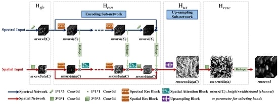
Figure 1.
Illustration of our 1D network architecture including the encoding sub-network and the up-sampling sub-network. The input of hyperspectral single image super-resolution (HSISR) are the low resolution (LR) Hyperspectral images (HSIs), and the inputs of hyperspectral pansharpening are LR HSI and pan. To ensure that both tasks can employ this network, the pan image used for hyperspectral pansharpening is simply addressed via a multi-scale learning network to extract deep spatial features, and then form a deep feature cube with the same size of the LR HSI. The detailed network and parameters setting for extraction of the deep features can be referenced from Figure 4 and Table 2.

Figure 2.
Illustration of 1D convolution path for spectral feature encoding, and 2D convolution path for spatial feature extraction of our proposed spectral and spatial residual block.
Figure 2.
Illustration of 1D convolution path for spectral feature encoding, and 2D convolution path for spatial feature extraction of our proposed spectral and spatial residual block.

Figure 3.
The detailed structures of our proposed spatial attention block.

Figure 4.
The spatial inputs of hyperspectral pansharpening that is reconstructed as the same size of LR HSI.
Figure 4.
The spatial inputs of hyperspectral pansharpening that is reconstructed as the same size of LR HSI.

Figure 5.
The performance of our proposed algorithm with the increasing a.

Figure 6.
The visual results of spatial super-resolution (SR) on Pavia University, in which the area in the red rectangle is enlarged three times in the bottom right corner of the image.
Figure 6.
The visual results of spatial super-resolution (SR) on Pavia University, in which the area in the red rectangle is enlarged three times in the bottom right corner of the image.

Figure 7.
The visual results of spatial SR on Pavia Center, in which the area in the red rectangle is enlarged three times in the bottom right corner of the image.
Figure 7.
The visual results of spatial SR on Pavia Center, in which the area in the red rectangle is enlarged three times in the bottom right corner of the image.

Figure 8.
Example spectrum of Pavia University: The figures above show the locations and the figures below show the corresponding spectrum.
Figure 8.
Example spectrum of Pavia University: The figures above show the locations and the figures below show the corresponding spectrum.

Figure 9.
Example spectrum of Pavia Center: The figures above show the locations and the figures below show the corresponding spectrum.
Figure 9.
Example spectrum of Pavia Center: The figures above show the locations and the figures below show the corresponding spectrum.

Figure 10.
The visual results of hyperspectral pansharpenning on the CAVE. dataset, in which the area in the red rectangle is enlarged three times in the bottom right corner of the image.
Figure 10.
The visual results of hyperspectral pansharpenning on the CAVE. dataset, in which the area in the red rectangle is enlarged three times in the bottom right corner of the image.

Figure 11.
Example spectrum of the Cave dataset: The figures above show the locations and the figures below show the corresponding spectrum.
Figure 11.
Example spectrum of the Cave dataset: The figures above show the locations and the figures below show the corresponding spectrum.

Figure 12.
The visual results of hyperspectral pansharpenning on the Harvard dataset, in which the area in the red rectangle is enlarged three times in the bottom right corner of the image.
Figure 12.
The visual results of hyperspectral pansharpenning on the Harvard dataset, in which the area in the red rectangle is enlarged three times in the bottom right corner of the image.

Figure 13.
Example spectrum of Havard dataset: The figures above show the locations and the figures below show the corresponding spectrum.
Figure 13.
Example spectrum of Havard dataset: The figures above show the locations and the figures below show the corresponding spectrum.


Table 1.
Parameters setting for the proposed attention based 1D–2D two-stream convolutional neural network (CNN).
Table 1.
Parameters setting for the proposed attention based 1D–2D two-stream convolutional neural network (CNN).
| Layer | Spectral Net | Spatial Net | Output Size |
|---|---|---|---|
| conv1 | |||
| res |
Table 2.
Parameters setting for the inputs of the spatial network of HSI pansharpening.
| Llayer | Kernel | Stride | Output Size |
|---|---|---|---|
| conv1+Prelu | |||
| Reshape | − | − | |
| conv2+Prelu | |||
| conv3+Prelu | |||
| conv3+Prelu | |||
| Concate | - | ||
Table 3.
Results on the pavia center dataset when r = 4 from different network architectures.
| Spa | Spe | 3D Conv | Spe-spa | Proposed | |
|---|---|---|---|---|---|
| (32) | (32) | (32) | (32,32) | (32,32) | |
| MPSNR (↑) | 30.605 | 30.509 | 31.099 | 31.249 | 31.306 |
| MSSIM (↑) | 0.8174 | 0.8165 | 0.8228 | 0.8222 | 0.8268 |
| MRMSE (↓) | 7.2291 | 7.3388 | 7.1928 | 7.1511 | 7.0625 |
| SAM (↓) | 3.9666 | 3.9650 | 3.9284 | 3.9170 | 3.8707 |
Table 4.
Parameters used in the Pavia Center dataset from different network architectures: , where r denotes the , , and .
Table 4.
Parameters used in the Pavia Center dataset from different network architectures: , where r denotes the , , and .
| Layer | Spa | Spe | 3D Conv | Spe-spa | Proposed | ||
|---|---|---|---|---|---|---|---|
| input | |||||||
| Conv+Prelu | |||||||
| ResBlock1 | |||||||
| Conv+Prelu | |||||||
| SaBlock1 | - | - | - | - | - | - | |
| ResBlock2 | |||||||
| Conv+Prelu | |||||||
| SaBlock2 | - | - | - | - | - | - | |
| ResBlock3 | |||||||
| Conv+Prelu | |||||||
| SaBlock3 | - | - | - | - | - | - | |
| Conv+Prelu | |||||||
| UpsamplingBlock | |||||||
| Conv+Prelu | |||||||
| Conv+Prelu | |||||||
| Reshape | Reshape | - | - | Reshape | Reshape | ||
| Total | 139532 | 96332 | 269708 | 161780 | 174456 | ||
| Output | |||||||
Table 5.
Quantity results on the Pavia University dataset.
| Up-Sampling | GDRRN | LapSRN | 3DFCN | Proposed | ||
|---|---|---|---|---|---|---|
| Pavia University | 2 | MPSNR (↑) | 33.348 | 34.797 | 34.956 | 36.705 |
| MSSIM (↑) | 0.9241 | 0.9412 | 0.9449 | 0.9648 | ||
| MRMSE (↓) | 5.4951 | 4.6660 | 4.5813 | 3.7003 | ||
| SAM (↓) | 3.9006 | 2.9373 | 3.0519 | 2.5385 | ||
| 4 | MPSNR (↑) | 28.431 | 29.046 | 29.323 | 30.262 | |
| MSSIM (↑) | 0.7811 | 0.8025 | 0.8095 | 0.8540 | ||
| MRMSE (↓) | 9.7096 | 9.0532 | 8.7808 | 7.9537 | ||
| SAM (↓) | 5.6290 | 4.6332 | 4.7339 | 4.2845 | ||
| 8 | MPSNR (↑) | 24.758 | 24.989 | 25.1381 | 25.953 | |
| MSSIM (↑) | 0.6085 | 0.6325 | 0.6363 | 0.6965 | ||
| MRMSE (↓) | 14.825 | 14.454 | 14.206 | 13.057 | ||
| SAM (↓) | 8.104 | 7.0909 | 7.1711 | 6.5839 |
Table 6.
Quantity results on the Pavia Center dataset.
| Up-Sampling | GDRRN | LapSRN | 3DFCN | Proposed | ||
|---|---|---|---|---|---|---|
| Pavia Center | 2 | MPSNR (↑) | 34.556 | 36.120 | 36.609 | 38.206 |
| MSSIM (↑) | 0.9177 | 0.9393 | 0.9436 | 0.9562 | ||
| MRMSE (↓) | 4.8165 | 4.0314 | 3.8193 | 3.1965 | ||
| SAM (↓) | 3.4740 | 2.6484 | 2.6683 | 2.4156 | ||
| 4 | MPSNR (↑) | 29.798 | 30.859 | 30.376 | 31.696 | |
| MSSIM (↑) | 0.7740 | 0.8083 | 0.8011 | 0.8446 | ||
| MRMSE (↓) | 8.3246 | 7.3942 | 7.7929 | 6.7142 | ||
| SAM (↓) | 4.8129 | 4.1540 | 4.2355 | 3.7263 | ||
| 8 | MPSNR (↑) | 27.039 | 27.399 | 27.318 | 28.104 | |
| MSSIM (↑) | 0.6531 | 0.6667 | 0.6590 | 0.6812 | ||
| MRMSE (↓) | 11.4716 | 11.0150 | 11.123 | 10.267 | ||
| SAM (↓) | 5.9319 | 5.5958 | 5.8345 | 5.3134 |
Table 7.
Quantitative comparison of hyperspectral pansharpenning of the Cave dataset.
| Up-Sampling | GFPCA | CNMF | Hysure | Proposed | ||
|---|---|---|---|---|---|---|
| Cave | 4 | ERGAS (↓) | 4.2216 | 3.3440 | 5.0781 | 2.0729 |
| MRMSE (↓) | 0.0186 | 0.0142 | 0.0222 | 0.0087 | ||
| SAM (↓) | 4.2283 | 4.1727 | 6.0103 | 2.7853 | ||
| CC(↑) | 0.9728 | 0.9788 | 0.9645 | 0.9889 |
Table 8.
Quantitative comparison of hyperspectral pansharpening of the Harvard dataset.
| Up-Sampling | GFPCA | CNMF | Hysure | Proposed | ||
|---|---|---|---|---|---|---|
| Harvard | 4 | ERGAS (↓) | 3.4676 | 2.6722 | 3.0837 | 2.2830 |
| MRMSE (↓) | 0.0140 | 0.0098 | 0.0108 | 0.0072 | ||
| SAM (↓) | 3.2621 | 3.0872 | 3.6035 | 3.1363 | ||
| CC(↑) | 0.9324 | 0.9454 | 0.9453 | 0.9597 |
© 2019 by the authors. Licensee MDPI, Basel, Switzerland. This article is an open access article distributed under the terms and conditions of the Creative Commons Attribution (CC BY) license (http://creativecommons.org/licenses/by/4.0/).
Share and Cite
MDPI and ACS Style
Li, J.; Cui, R.; Li, B.; Song, R.; Li, Y.; Du, Q. Hyperspectral Image Super-Resolution with 1D–2D Attentional Convolutional Neural Network. Remote Sens. 2019, 11, 2859. https://doi.org/10.3390/rs11232859
AMA Style
Li J, Cui R, Li B, Song R, Li Y, Du Q. Hyperspectral Image Super-Resolution with 1D–2D Attentional Convolutional Neural Network. Remote Sensing. 2019; 11(23):2859. https://doi.org/10.3390/rs11232859
Chicago/Turabian StyleLi, Jiaojiao, Ruxing Cui, Bo Li, Rui Song, Yunsong Li, and Qian Du. 2019. "Hyperspectral Image Super-Resolution with 1D–2D Attentional Convolutional Neural Network" Remote Sensing 11, no. 23: 2859. https://doi.org/10.3390/rs11232859
Note that from the first issue of 2016, this journal uses article numbers instead of page numbers. See further details here.