Automated Built-Up Extraction Index: A New Technique for Mapping Surface Built-Up Areas Using LANDSAT 8 OLI Imagery

Abstract

Accurate built-up area extraction is one of the most critical issues in land-cover classification. In previous studies, various techniques have been developed for built-up area extraction using Landsat images. However, the efficiency of these techniques under different technical and geographical conditions, especially for bare and sandy areas, is not optimal. One of the main challenges of built-up area extraction techniques is to determine an optimum and stable threshold with the highest possible accuracy. In many of these techniques, the optimum threshold value fluctuates substantially in different parts of the image scene. The purpose of this study is to provide a new index to improve built-up area extraction with a stable optimum threshold for different environments. In this study, the developed Automated Built-up Extraction Index (ABEI) is presented to improve the classification accuracy in areas containing bare and sandy surfaces. To develop and evaluate the accuracy of the new method for built-up area extraction with Landsat 8 OLI reflective bands, five test sites located in the Iranian cities (Babol, Naqadeh, Kashmar, Bam and Masjed Soleyman), eleven European cities (Athens, Brussels, Bucharest, Budapest, Ciechanow, Hamburg, Lyon, Madrid, Riga, Rome and Porto) and high resolution layer imperviousness (HRLI) data were used. Each site has varying environmental and complex surface coverage conditions. To determine the optimal weights for each of the Landsat 8 OLI reflective bands, the pure pixel sets for different classes and the improved gravitational search algorithm (IGSA) optimization were used. The Kappa coefficient and overall error were calculated to evaluate the accuracy of the built-up extraction map. Additionally, the ABEI performance was compared with the urban index (UI) and normalized difference built-up index (NDBI) performances. In each of the five test sites and eleven cities, the extraction accuracy of the built-up areas using the ABEI was higher than that using the UI, and NDBI (P-value of 0.01). The relative standard deviations of the optimal threshold values for the ABEI and UI were 27 and 155% (at five test sites) and were 16 and 37% (at eleven European cities), respectively, which indicates the stability of the ABEI threshold value when the location and environmental conditions change. The results of this study demonstrated that the ABEI can be used to extract built-up areas from other land covers. This index is effective even in bare soil and sandy areas, where other indices experience major challenges.

1. Introduction

Urban areas generally cover a small portion of land worldwide. However, the high population density and intensity of utilizing resources relative to their surroundings turn these areas into highly important land areas [1,2]. Understanding the spatial distribution and growth pattern of urban built-up areas is vital for urban planning, natural resource management, climate change monitoring, etc., and the ecological, economic and social effects of built-up lands have made the mapping of built-up areas very important [2,3,4,5,6].

Satellite images are a valuable source for built-up mapping in areas with different environmental conditions [7,8,9,10,11,12]. Remote sensing technology provides an integrated, comprehensive view of urban areas that is difficult to achieve through surveying. Another advantage of using remote sensing data for urban studies is the availability of archives of past periods that can be used to review, monitor, and prepare a distribution map of built-up areas over time [13,14]. Over recent years, satellite imagery capabilities have been used for studies on urban expansion [15], effective factors on urban development [16], and the negative effects of urban growth [17].

Generally, in previous studies for mapping built-up areas usually coarse-resolution satellite imagery such as moderate resolution imaging spectroradiometer (MODIS) [18,19] and defense meteorological program / operational line-scan system (DMSP/OLS) [20], medium-resolution satellite imagery such as Landsat [21] and Sentinel-2 [22], and high-resolution satellite imagery such as Quick Bird [23] and WorldView [24] have been used. Landsat imagery has the potential to provide a historical record for mapping built-up areas, as Landsat has been acquiring images since the early 1980s. Landsat imagery has been used frequently to extract built-up areas in urban studies [25]. Its large coverage, suitable spatial resolution (30 m), historical observations and free access have proved that Landsat imagery is useful for mapping built-up areas [1,2,25].

Currently, satellite imagery is increasingly being used automatically and semi-automatically to generate various maps of land surface characteristics, such as vegetation, snow, water and built-up land characteristics [26,27,28,29,30]. Several techniques have been developed for this purpose, which are grouped into two general categories. The first group relates to image classification techniques, which have been widely developed based on pixel-based and object-oriented classification methods [13,31]. The second group involves information extraction from images based on specific indices [2]. Both groups of techniques have a set of advantages and disadvantages. The accuracy of classification methods may be higher than indices, but, in general, the use of indices in a case of certain land-cover extraction according to the amount of information, need to train data, and time required for processing is more efficient than the use of classification techniques.

Different indices have been developed for built-up area extraction using satellite imagery [2,7,8,9,11,29]. The basis of the development of these indices is the spectral behaviour of the built-up land and various features associated with the wavelengths of the electromagnetic spectrum in terms of absorption or reflection. Different bands of the satellite image represent the different wavelengths of the electromagnetic spectrum. Accordingly, these indices have been developed with a special combination of image bands. Investigating and studying the spectral signatures of various features are necessary to create and develop various indices related to the identification and extraction of these phenomena [26].

In previous studies, different indices, such as the index-based built-up index (IBI) [12], urban index (UI) [32,33], normalized difference bareness index (NDBaI) [33], normalized difference built-up index (NDBI) [29], modified NDBI [9], normalized built-up area index (NBAI) and band ratio for built-up area (BRBA) [11], new built-up index (NBI) [8], built-up index (BUI) [10], bare soil index (BI) [34], enhanced built-up and bareness index (EBBI) [7], and built-up area extraction method (BAEM) [2], have been developed for built-up and urban area mapping.

Kawamura et al. (1996) proposed the UI for mapping built-up areas. The UI is computed by using the bands 7 and 4 from Landsat Thematic Mapper (TM) imagery [32]. Zha et al. (2003) developed the NDBI for the automatic mapping of built-up areas. They extracted built-up areas through arithmetic calculation using the NDVI and NDBI derived from Landsat TM images. In the binary images created by the NDBI and NDVI images via this technique, it is assumed that positive values of the NDBI indicate built-up areas and that positive NDVI values indicate vegetation covers. Zha et al. (2003) reported that their method is incapable of separating built-up areas from bare land [29]. As-syakur et al. (2012) developed the EBBI for mapping built-up and bare land in urban areas. They extracted built-up and bare land areas through single calculation using near infrared (NIR), short wave infrared (SWIR), and thermal infrared (TIR) bands simultaneously [7]. Waqar et al. (2012) developed NBAI and BRBA Indices for mapping built-up area and bare soil covers using Landsat TM images. They extracted built-up areas through NBAI using the bands 2, 5 and 7 of Landsat TM images. Also, they extracted built-up areas through BRBA using the ratio of bands 3 and 5 of Landsat TM images [11]. Kaimaris and Patias (2016) developed the BUI based on the combination of the bands 3, 5 and 7 of Landsat Enhanced Thematic Mapper Plus (ETM+) images. In BUI, unlike other indices, the NIR band was not used for mapping built-up areas [10]. The IBI was distinguished from other built-up indices because of its first-time use of thematic indices rather than using original bands. The soil adjusted vegetation index (SAVI), modified normalized difference water index (MNDWI) and NDBI indices were used in IBI [12].

The NDBI and UI provide quick mapping of built-up areas or bare land. However, these two indices are unable to separate built-up areas from bare land effectively [9,29,35]. He et al. [9] noted in their study that this incapability was due to the complex spectral response generated by the combination of the spectral responses of built-up areas, vegetation and bare land, especially in terms of mixed pixels in areas with heterogeneous features.

Having reviewed previous studies in this field of study, it is clear that most of the developed indices are effective in mapping bare land and built-up areas, but these indices are not able to completely isolate built-up and bare lands in the same area [7]. In different areas, the performances of these indices are affected by the type of land use in the region. Therefore, these indices have problems in distinguishing between built-up and other land use areas that have similar spectral behaviours. Even the spectral heterogeneity between pixels related to built-up areas reduces the accuracies of the indices. Generally, the accuracies of these indices for built-up area extraction are low [10]. For this reason, in some studies, several different indices have been combined with built-up area extraction [2].

Simplified techniques, such as two-band indices and single-band thresholding, may not accurately separate built-up pixels from non-built-up bright surfaces, particularly in scenes where non-built-up bright surfaces are seen. Current built-up extraction methods have accuracy problems in distinguishing built-up areas from bare land and rock surfaces [2,7,8,29]. It is worth mentioning that no existing built-up index has been capable of automatically separating built-up and bare lands using Landsat 8 OLI (Operational Land Imager) images. Therefore, in this study, a multiple-band index, called the Automated Built-up Extraction Index (ABEI), was introduced with two main objectives: (1) increase the accuracy of built-up extraction mapping by automatically separating built-up areas from other non-built-up bright surfaces and (2) test the novel technique under various environmental conditions and assess its accuracy in comparison with other techniques.

The major distinctions between the present study and other studies in this field are (1) the development of a new index for built-up extraction using all of the Landsat 8 OLI reflective bands, (2) the use of the improved gravitational search algorithm (IGSA) optimization to determine the relevant weights in different reflective bands and (3) the use of the stable optimum threshold value for the classification of built-up areas under different environmental conditions and various surfaces.

2. Test Sites and Cities

To perform an accuracy assessment with the new technique for automatic built-up extraction from Landsat 8 OLI reflective bands, 5 test sites with different environmental conditions and complex land covers were selected. Test sites from Babol, Naqadeh, Kashmar, Bam and Masjed Soleyman are included and located in different geographical locations with different climatic conditions in Iran. The characteristics of the test sites are shown in

Table 1. General characteristics of the test sites and cities.

Test Site and City	Centre Point Coordinate (Lon, Lat-WGS84)	Country	Area (Km2)	Mean Alt. (m)	Climate	Population (2019)
	Test sites
Babol	52.68, 36.54	Iran	2.0	3	Humid	>5600
Naqadeh	45.38, 36.95	Iran	0.5	1325	Semi-humid	>1500
Masjed Soleyman	49.28, 31.96	Iran	3.4	240	Dry and semi-arid	>6500
Kashmar	58.46, 35.24	Iran	5.4	1060	Warm and dry	>7000
Bam	58.33, 29.10	Iran	1.3	1083	Warm and dry	>2800
	European cities
Rome	12.45, 41.85	Italy	631.7	50	Mediterranean	>4,234,000
Riga	24.09, 56.94	Latvia	558.0	10	Humid continental	>633,000
Madrid	−3.70, 40.41	Spain	2332.3	650	Mediterranean and semi-arid	>6,559,000
Athens	23.72, 37.97	Greece	2142.2	80	Mediterranean	>3,154,000
Brussels	4.38, 50.85	Belgium	608.1	60	Oceanic	>2,065,000
Porto	−8.60, 41.16	Portugal	481.4	80	Mediterranean	>1,309,000
Lyon	4.83, 45.76	France	1143.6	175	Humid subtropical	>1,704,000
Ciechanow	20.60, 52.82	Poland	81.1	151	Humid subtropical	>44,000
Hamburg	10.02, 53.60	Germany	1097.5	10	Oceanic	>1,791,000
Budapest	19.07, 47.59	Hungary	3664.3	120	Oceanic and Humid subtropical	>1,763,000
Bucharest	26.10, 44.42	Romania	1385.7	85	Humid continental	>1,812,000

.

The test sites are selected in the form of complex features in terms of spectral properties, such as soil, sand, and rock properties. The Babol and Naqadeh test sites are selected due to their humid and semi-humid climates, including built-up, agricultural, water, soil, and dense vegetation covers. The Kashmar and Bam test sites are selected due to their warm and dry climates, including built-up, bare land, sandy soil and vegetation covers. The test site of Masjed Soleyman is a mountainous region with a semi-arid climate, including built-up, bare land and rock surfaces.

To broadly evaluate the ABEI performance in different geographical locations with different environmental conditions, the ABEI were implemented on 11 European cities including Athens, Brussels, Bucharest, Budapest, Ciechanow, Hamburg, Lyon, Madrid, Riga, Rome and Porto. The cities are selected to cover different geographical locations and climatic conditions across Europe. Among the selected cities, Athens, Riga, Rome and Porto are Coastal cities. The areas around Athens and Madrid include bare land. The Brussels, Budapest, Bucharest, Ciechanow, Hamburg, Lyon, Riga and Porto have high vegetation cover due to humid climates. Above all, the main reason for selecting these cities in Europe was the absence of cloud-free Landsat 8 OLI images in 2015. In summary, the characteristics of the European cities are listed in Table 1. The geographical locations of the test sites and European cities are shown in Figure 1.

3. Data and Methods

3.1. Landsat Images and Reference Data

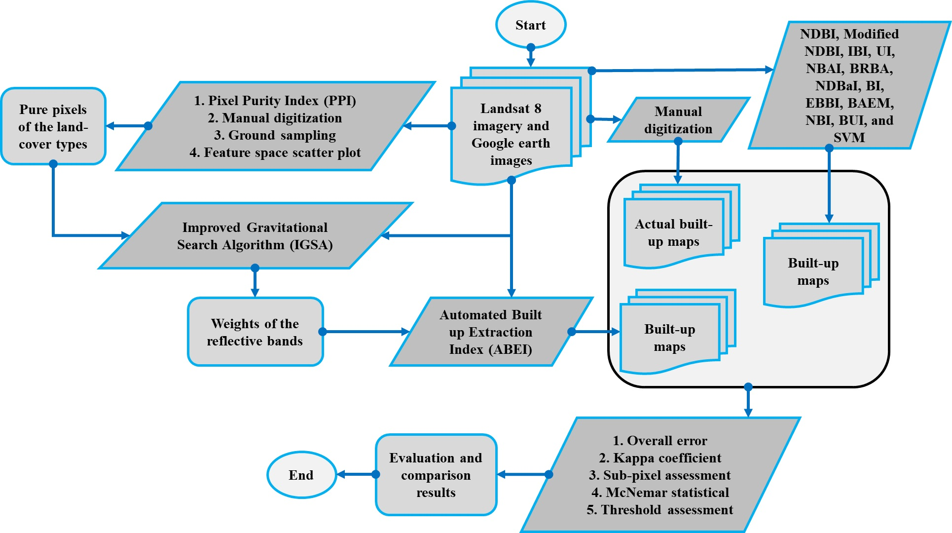
In the present study, the reflective bands of the satellite images acquired by Landsat 8 OLI were used. The satellite images with no cloud cover and no rainfall within 2 days before satellite overpass were selected. The images were georeferenced in the UTM coordinate system. The downloaded data from USGS included the highest quality Level-1 Precision Terrain (L1TP) data, which were considered suitable for time-series analysis. The geo-registration was consistent, and the root mean square error (RMSE) was less than 12 m (≤0.5 pixel) [36]. For each of the five test sites, high-spatial-resolution Google Earth Images were used as reference data. The times for the reference data and Landsat 8 OLI images used in this study were very similar at the test sites. To digitize and extract built-up areas from Google Earth images, a photointerpretation method was used. The derived built-up map was used to accurately assess the different build-up extraction methods.

Additionally, the high resolution layer imperviousness (HRLI) data have been used as reference data to evaluate ABEI performance in European cities. The HRLI data provided by the Copernicus Global Land Service (CGLS) had a pixel resolution of 20 m. The HRLI data were generated based on IRS-P6/Resourcesat-2 LISS-III, SPOT 5 and Landsat 8 data sets for different regions of Europe. These reference data for 2006, 2009, 2012 and 2015 are available at the https://land.copernicus.eu/ website. The results of applying the ABEI on the Landsat 8 OLI imagery from European cities were evaluated with the HRLI data of 2015 for each city. Details of the Landsat images and reference data are presented in

Table 2. Description of the Landsat 8 OLI scenes and corresponding reference data.

Test Site	Landsat Scene			Reference Data and Sources
	Acquisition Date	Path	Row
Babol	1 May 2015	164	35	Google Earth™ image acquired on 29 April 2015, ©Digital Globe
Naqadeh	13 August 2014	169	34	Google Earth™ image acquired on 10 August 2014, ©Digital Globe
Masjed Soleyman	15 August 2016	165	38	Google Earth™ image acquired on 14 August 2016, ©Digital Globe
Kashmar	14 October 2016	160	35	Google Earth™ image acquired on 14 August 2016, ©CNES/Airbus
Bam	6 May 2018	159	40	Google Earth™ image acquired on 9 May 2018, ©Digital Globe
Cities
Rome	17 July 2015	191	031	High Resolution Layer Imperviousness (HRLI) for the 2015 reference year, European Environment Agency
Riga	9 May 2015	188	020
Madrid	7 July 2015	201	032
Athens	26 August 2015	180	031
Brussels	11 September 2015	199	025
Porto	12 July 2015	204	031
Lyon	12 August 2015	197	028
Ciechanow	4 August 2015	189	023
Hamburg	21 August 2015	196	023
Budapest	29 August 2015	188	027
Bucharest	3 August 2015	189	029

.

3.2. Methods

3.2.1. Image Preprocessing

Atmospheric correction of satellite imagery was performed using the Fast Line-of-sight Atmospheric Analysis of Hypercubes (FLAASH) algorithm [37]. This module employs the MODTRAN 6 model [38]. To this end, some parameters, such as the satellite overpass time, the sensor altitude, the geographical location, the specific atmospheric model related to the region, and the solar zenith angle, are considered. For each of the five test sites, the aerosol optical depth (AOD) and total water vapor content in the atmosphere used in the FLAASH algorithm were derived from the Terra MODIS atmospheric profile product, which was collected by the Terra platform [18]. The overpass times of Terra and Landsat 8 approximately match each other (less than a 2 h difference). There was no need for manual co-registration because the co-registration between the Landsat and Google Earth images at the test sites was accurate.

3.2.2. Formulation of the Automated Built up Extraction Index (ABEI)

Landsat 8 OLI reflective bands (7 bands) were used to develop the ABEI. The purpose of the ABEI is to create maximum similarity between the pixel values of the built-up class and the maximum difference between the pixel values of the built-up class and other land-cover classes. For this purpose, the combination of the reflective bands of Landsat 8 OLI and the weight of each band are used, as shown in Equation (1).

$$A\mathrm{BEI}={\mathsf{\mu }}_1{\mathrm{Ref}}_1+{\mathsf{\mu }}_2{\mathrm{Ref}}_2+{\mathsf{\mu }}_3{\mathrm{Ref}}_3+{\mathsf{\mu }}_4{\mathrm{Ref}}_4+{\mathsf{\mu }}_5{\mathrm{Ref}}_5+{\mathsf{\mu }}_6{\mathrm{Ref}}_6+{\mathsf{\mu }}_7{\mathrm{Ref}}_7$$

(1)

In this study, IGSA optimization was applied to determine the weights of the reflective bands (${\mathsf{\mu }}_1$, ${\mathsf{\mu }}_2$, ${\mathsf{\mu }}_3$, ${\mathsf{\mu }}_4$, ${\mathsf{\mu }}_5$, ${\mathsf{\mu }}_6$ and ${\mathsf{\mu }}_7$). To implement IGSA optimization for determining the optimal weights of different bands applicable to all areas, a pure pixel data set of surface covers and a specific objective function were used. The objective function in the IGSA optimization to determine the scale of the feature space considered (weights of different bands) is defined in Equation (2), where $\Delta ABE{I}_{i{M}_i}$ is the distance (difference) between the ABEI value of the i-th built-up training sample and the built-up cluster centre ($M_i$) (Mean ABEI values of built-up samples) and $\Delta ABE{I}_{i{M}_{nearest}}$ is the distance (difference) between the ABEI value of the i-th built-up training sample and the nearest neighbour cluster centre ($M_{nearest}$) (Mean ABEI values of each land cover samples were calculated (cluster centre for each land cover was obtained). The difference of ABEI value of a built-up sample and other land cover cluster centre was calculated. The minimum value of difference determines the nearest neighbour cluster centre to a built-up sample).

$$F_{obj} ={\displaystyle \sum }_{ i=1:T}\frac{\Delta ABE{I}_{i{M}_i}}{ \Delta ABE{I}_{i{M}_{nearest}}}$$

(2)

In Equation (2), T is the total number of selected training samples for the built-up area. The purpose of IGSA optimization is to search the space for all possible states that allow the coefficient values of ${\mathsf{\mu }}_1$, ${\mathsf{\mu }}_2$, ${\mathsf{\mu }}_3$, ${\mathsf{\mu }}_4$, ${\mathsf{\mu }}_5$, ${\mathsf{\mu }}_6$ and ${\mathsf{\mu }}_7$ to reach the optimal value (minimum) for the objective function. This objective function establishes a balance in the feature space in such a way that the maximum homogeneity of ABEI values between built-up pixels and the maximum difference of the ABEI values between built-up pixels and other land-cover classes can be established. Additionally, by finding the optimum value for this objective function and using the pure pixels of different land-cover classes, the threshold values are also close to each other for different dates and regions. Therefore, the effective feature vectors and their scales can be predicted and we can use them to achieve the best accuracy of the built-up area classification. Main reasons for employing the IGSA algorithm instead of other optimization algorithms in this study are: (a) in many optimization algorithms, the initial population does not cover some parts of problem space. Therefore, optimization algorithms face challenges to find the optimum location in problem space. However, IGSA is able to remove this problem with negative mass; (b) The process time to achieve the optimum coefficients in IGSA compared to other algorithms is short; (c) the IGSA properties such as the memory and using the negative mass significantly decrease the occurrence possibility of local minima and search in a more efficient way the problem space.

3.2.3. Pure-Pixel Selection

To extract the surface reflectance values for 8 different land covers, 7 reflective bands of the Landsat 8 OLI images of the test sites and surrounding areas were sampled. The types of surface covers include built-up, vegetation, bare land, sandy soil, rock, agricultural and water land covers. Given that the spectral values related to the pure pixels of surface covers directly affect the accuracy of the results of the built-up extraction, this stage is one of the most important stages of the study. For each of the surface covers, 150 pure pixels were extracted from 7 reflective bands of the Landsat 8 OLI images.

The set of methods includes photointerpretation from Google Earth images, ground sampling, the pixel purity index (PPI) and selection from the feature space scatter plot used to extract pure pixels of the land-cover types. Spectral separability of the selected land-cover classes was tested by the Jeffries–Matusita distance separability measure [39]. All pairs of land-cover classes, with values ranging from 1.76 to 2.01 were separable from each other.

3.2.4. Improved Gravitational Search Algorithm

In the IGSA, optimization was accomplished through the application of gravitational laws and motion in a synthetic discrete-time system. The system environment is the same as the definition of the problem. According to the law of gravity, every object is able to understand the location and situation of other objects through the law of gravitational attraction. Therefore, this force can be utilized as an instrument to exchange information. The designed optimum finder can be used to solve every optimization problem in which each solution is defined as a situation in space, and its similarity to the other solutions was expressed as a distance. The mass amounts were determined by the objective function. More detail about IGSA optimization can be found in [40].

3.2.5. Classification, Threshold Optimization and Per-Pixel Accuracy Assessment

To compare the accuracy of the ABEI with those of other indices, in the present study, indices such as the NDBI, modified NDBI, IBI, UI, NBAI, BRBA, NDBaI, BI, EBBI, BAEM, NBI and BUI were applied. The results of applying these indices on the data from the test sites proved that the UI has been more efficient in built-up extraction. For this reason, only the UI performance was compared with the ABEI performance in this study.

According to the ABEI, a default value of the threshold equal to zero is used to separate built-up and non-built-up pixels. Pixels with a value greater than zero are built-up areas, and pixels with values less than zero are non-built-up areas. However, due to different environmental conditions in different regions, the threshold values for both the ABEI and UI indices were determined according to the reference map for test sites and based on the overall error parameter. For this purpose, the threshold value was changed to 0.001, and with each change, the value of the overall error parameter was calculated. Finally, the optimal threshold for each test site was calculated with the condition of minimizing the overall error value. To assess the stability of the ABEI and UI threshold values, the changes in the optimal threshold values for the two indices applied to the test sites were investigated based on relative standard deviation criteria. To compare the accuracies of the ABEI, and UI the overall errors and Kappa coefficients were calculated based on confusion matrices. To compare the ABEI and UI accuracies, the results from the optimal threshold values of each index were used.

Additionally, to investigate whether the ABEI remarkably improves accuracy compared to the UI method at these test sites, the McNemar statistical test was applied. According to Equation (3), McNemar’s continuity-corrected chi-square statistic was calculated as [41]:

$$X^2=\frac{{\left(\left|f_{12}-f_{21}\right|-1\right)}^2}{f_{12}-f_{21}}$$

(3)

where $f_{12}$ and $f_{21}$ define the frequencies of pixels that were correctly classified by one method but incorrectly classified by the other, respectively.

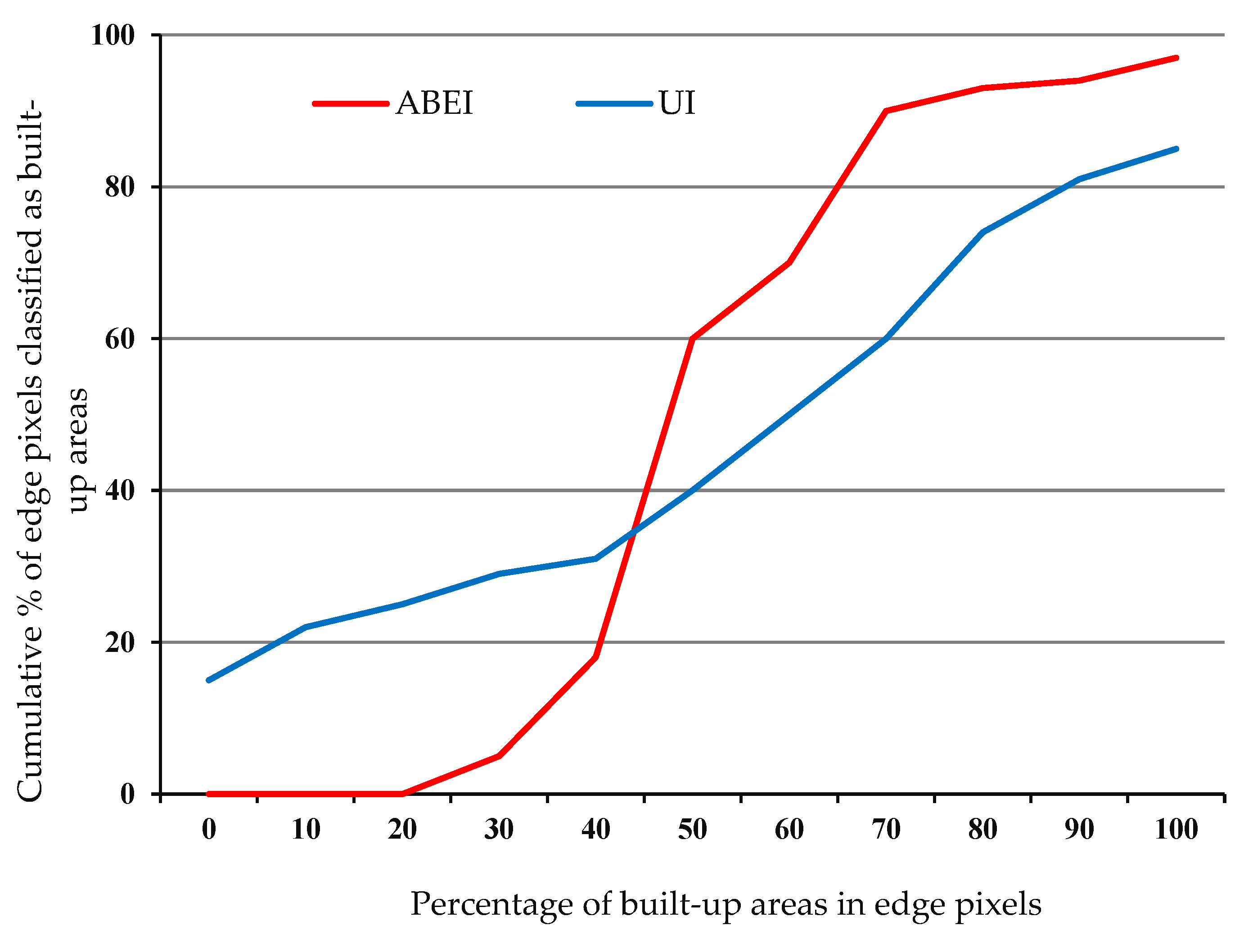
3.2.6. Mixed Pixel (Heterogeneous Region) Accuracy Assessment

The sensitivity and efficiency of different classifiers for the accurate classification of mixed pixels of built-up and non-built-up lands were evaluated using the overall accuracy assessment for mixed pixels and boundary regions. For this assessment, 1800 mixed pixels of the 5 test sites were selected. Using Google Earth Images for each test site, the percentages of built-up and non-built-up areas for each pixel were computed. Then, the pixels were classified into 10 classes based on the percentage of built-up area. Finally, the percentages of pixels of each class classified by each of the three methods (ABEI and UI) for built-up areas were calculated. Ideally, if the percentage of built-up areas in a pixel is higher than 50%, this pixel should be classified in the built-up class and, conversely, the opposite is classified in the non-built-up class.

3.2.7. The Performance Evaluation of ABEI Using Cross-Validation Analysis

In this study, HRLI reference data were used for the final evaluation of the ABEI performance for mapping surface built-up areas. The results of ABEL were compared with HRLI reference maps of 2015 for European cities. Finally, the overall accuracy of the built-up map extracted by ABEI was computed based on reference map for each city. Also, the performance of ABEI was compared with NDBI and UI for mapping built-up areas in European cities based on reference maps. Finally, the changes of optimal threshold values for built-up extraction with ABEI, UI and NDBI were analyzed for the different European cities.

4. Results

4.1. ABEI

The aim of the ABEI is to create the greatest similarity between pixel values within the built-up class and the greatest difference in pixel values between the built-up class and other classes. In this study, using IGSA optimization, the objective function and pure pixels of different surface land covers and the optimal coefficients for each reflective band were obtained. The obtained ABEI is shown in Equation (4).

$$A\mathrm{BEI}=0.312{\mathrm{Ref}}_1+0.513{\mathrm{Ref}}_2-0.086{\mathrm{Ref}}_3-0.441{\mathrm{Ref}}_4+0.052{\mathrm{Ref}}_5-0.198{\mathrm{Ref}}_6+0.278{\mathrm{Ref}}_7$$

(4)

According to Equation (4), the coefficient value for each spectral band indicates the extent of the effect of each spectral band on built-up area extraction. It should be noted that in this technique, simultaneously with applying NDVI, water pure pixels (NDVI < 0) and vegetation pure pixels (NDVI > 0.5) were classified into the non-built-up class and in the built-up extraction process with ABEI were not included.

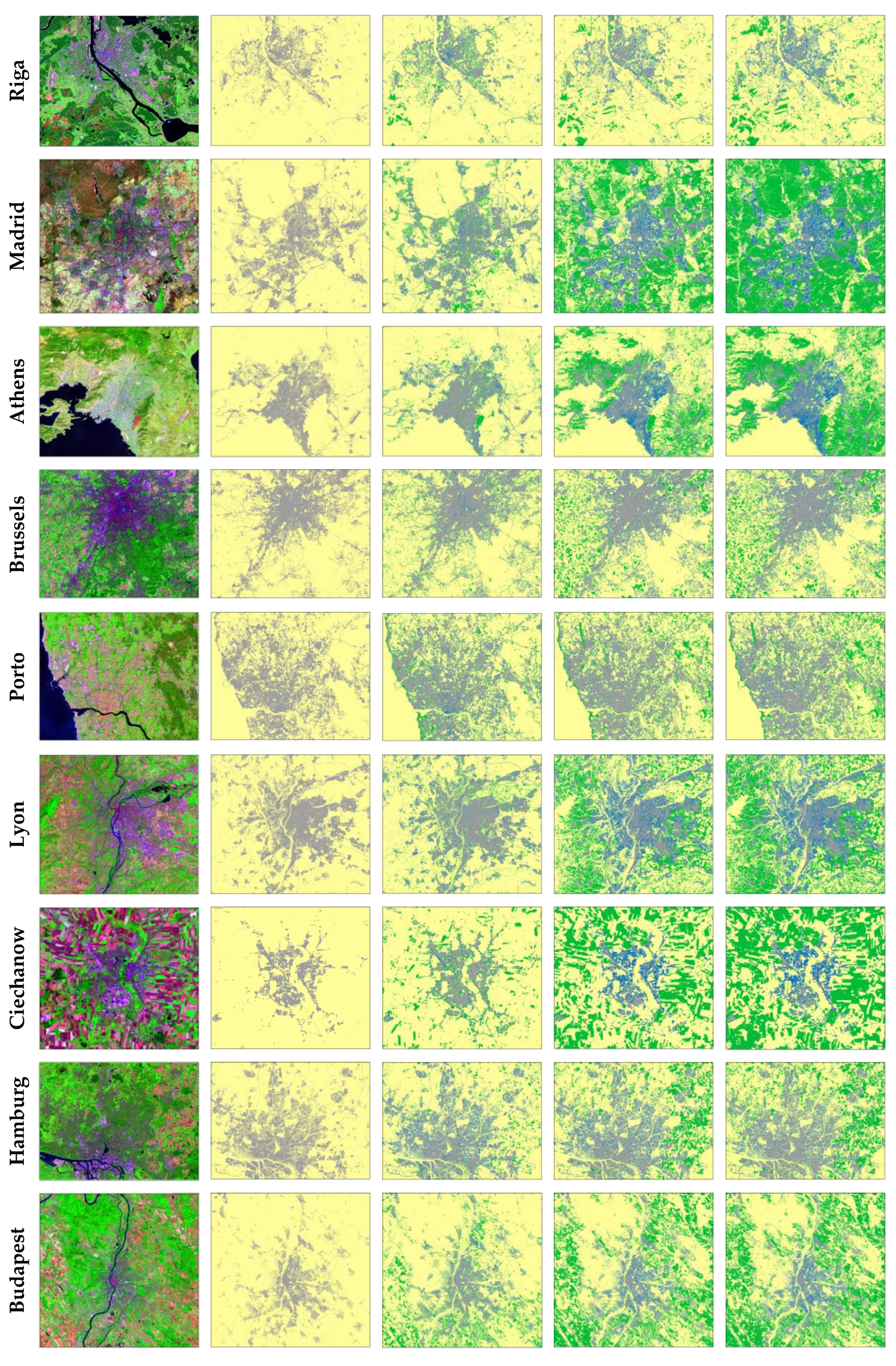
4.2. Built-Up Extraction Maps

The results of the two classification methods for the five test sites were shown in Figure 2. The visual assessment of Figure 2 demonstrates that the accuracy of the built-up extraction map extracted by the ABEI is better than that extracted by the UI. In each of the five test sites, the results of the UI are noisy. However, for the Naqadeh and Babol test sites, there are fewer differences between the classification methods in terms of built-up extraction. However, for the Bam, Kashmar and Masjed Soleyman test sites, due to their bare land, sandy soil and rocky surfaces, there is a remarkable difference between the results of the ABEI and those of the other methods. A visual examination of the results indicates that the increase in ABEI efficiency compared to the UI efficiencies at the arid test sites, including bare land and sandy areas, is more than that at the humid test sites. The main reason is the limitations that other methods have with bare lands. At the Bam site, due to the complexity of the region and the presence of bare lands, sandy soils and desert surfaces, the UI has a very low efficiency in built-up extraction.

The visual assessment of these results illustrates the higher efficiency of the ABEI for built-up extraction under bare land and sandy soil conditions.

4.3. Classification Accuracy and Edge Pixel Effects

The Kappa coefficient and overall accuracy of the built-up maps obtained for each test site were shown in

Table 3. Summary of the classification accuracies of the various methods by test site.

Test Site	Babol		Naqadeh		Masjed Soleyman		Kashmar		Bam
	Kc	OA	Kc	OA	Kc	OA	Kc	OA	Kc	OA
ABEI	0.93	94.01	0.96	97.62	0.94	95.95	0.92	93.34	0.9	92.04
UI	0.87	89.21	0.90	92.54	0.82	83.02	0.82	85.89	0.69	73.88
NDBI	0.84	86.16	0.86	87.12	0.78	79.92	0.79	80.65	0.66	86.34
IBI	0.73	74.32	0.74	75.23	0.68	68.91	0.70	71.36	0.59	74.23
NBAI	0.78	75.65	0.79	80.32	0.70	71.24	0.69	70.54	0.60	61.63
BRBA	0.74	75.36	0.73	74.53	0.69	70.32	0.70	71.25	0.58	59.41
NDBaI	0.73	74.63	0.75	75.96	0.69	71.01	0.68	69.69	0.53	54.74
BI	0.75	76.81	0.78	79.86	0.62	63.45	0.66	67.31	0.55	56.81
EBBI	0.82	83.12	0.81	82.31	0.76	77.98	0.75	76.85	0.64	65.45
BAEM	0.81	82.54	0.79	80.45	0.75	76.31	0.76	77.65	0.63	64.85
NBI	0.75	76.75	0.79	80.23	0.70	71.65	0.63	63.87	0.57	58.96
BUI	0.74	75.96	0.75	76.87	0.71	72.26	0.65	66.23	0.60	61.32

. For all test sites, the accuracy obtained by the ABEI is higher than that obtained by the UI. According to Figure 3, the average total omission and commission errors at the five test sites by the ABEI, and UI are 15.21, and 58.2%, respectively. Additionally, the standard deviations in the average of total omission and commission errors by the ABEI, and UI methods are 2.9, and 26.08%, respectively. The standard deviation values indicate that the ABEI method error compared to the mean error has a small difference. However, UI errors have large differences. In other words, the results of the accuracy assessment indicate the high stability of the accuracy of the ABEI at all test sites with different environmental conditions and surfaces in contrast to the UI method.

A summary of the classification accuracies of the various methods by test site is shown in

Table 4. McNemar chi-square test results for the five test sites.

Test Sites		Χ2	p-Value
	Classifier	UI	UI
Babol	ABEI	26.03	0
Naqadeh	ABEI	20.04	0
Masjed Soleyman	ABEI	288	0
Kashmar	ABEI	749	0
Bam	ABEI	27.03	0

.

The difference between the accuracies and errors of the built-up extraction methods among the test sites is different. This is because of the differences in the complexities of the surface land cover at various test sites. The difference among the overall accuracies of the built-up extractions by three methods at the Babol and Naqadeh test sites is low, but for the Kashmar and Bam test sites, this difference is very high. The McNemar chi-square test results for the five test sites were shown in Table 4.

According to the Table 4, the improvement in the accuracy of the ABEI was significant (p-value < 0.01 at the 99% confidence level) compared to those of the UI at all test sites. For test sites where the difference in the built-up extraction accuracy of the ABEI compared to those of other methods is low, the McNemar chi-square value is also low. The results of the subpixel accuracy assessment using various methods were shown in Figure 4.

The results indicate that the abilities of the ABEI, and UI to correctly classify pixels with various percentages of built-up areas are different. In general, with the ABEI, 60% of the mixed pixels were classified correctly into the built-up class. Using the UI method, due to the lack of completely distinguishing bare lands, sandy soils, and rock surfaces from built-up areas, an average of 24.5% of the pixels with less than 50% built-up areas were classified in the built-up class. Additionally, using the UI, an average of 30% of pixels with more than 50% built-up areas were classified into the non-built-up class. However, because of the objective function defined in the optimization algorithm that determines the optimal weight of each spectral band in the ABEI, the capability of this index is high for separating built-up areas from bare lands, sandy soils and rock surfaces. For this reason, with this method, only 4.6% of pixels with less than 50% built-up areas are classified into the built-up class, and on average, 11.2% of pixels with more than 50% built-up areas were classified into the non-built-up class.

4.4. Optimal Threshold and Its Variability

The comparison results for the stability of the optimal threshold values for the ABEI and UIwere shown in Figure 5.

The results indicate that the optimal threshold values for the different test sites using the UI compared to those using the ABEI experience more changes. For example, at the Babol and Naqadeh test sites, the optimal threshold value for the UI has changed from −0.1 to −0.02, and that for the ABEI has changed from 0.3 to 0.232. Generally, the relative standard deviations of the optimal threshold values at the test sites using the UI and ABEI are 155 and 27%, respectively. The lower relative standard deviation of the optimal threshold values for the ABEI compared to those for the UI represents more stability of the threshold value with spatial and temporal variations.

The advantages of the ABEI include a simple method and systematic technique for the precise separation of built-up areas from other surface land-cover classes, such as bare land, sandy soil and rock surfaces. The advantages of the new index in comparison with other indices in this field are the relatively high stability of the optimum threshold value with respect to the changes in spatial, temporal, and environmental conditions and surface land cover for the separation of built-up areas from non-built-up areas.

4.5. Cross-Validation Analysis

The results of the ABEI, UI and NDBI indices for the eleven European cities are shown in Figure 6. Based on the HRLI reference map of each city, the results of indices were evaluated. The blue pixels in each map represent omission errors and the green pixels in each map represent commission errors.

The visual assessment of Figure 6 demonstrates that the accuracy of the built-up extraction map extracted by the ABEI is better than that extracted by the UI and NDBI. Additionally, there is a significant difference between the results of the ABEI and those of the other indices in case of separation between built-up and bare land areas. A summary of the overall accuracies of the three indices by city was shown in Figure 7.

The mean value of overall accuracy at the eleven European cities using the ABEI, UI and NDBI is 89.3, 72.4 and 64.7%, respectively. The results indicate the high efficiency of ABEI for mapping built-up areas in absolute and relative terms according to UI and NDBI results. The most highest overall error of the UI and NDBI is seen in Madrid (48 and 67%, respectively). In general, the overall accuracies of the built-up extraction using the UI and NDBI are low in areas that covers with bare land. However, ABEI has good performance for separating built-up areas from other surface land-cover classes. The comparison results for the stability of the optimal threshold values for the ABEI, UI and NDBI were shown in Figure 8.

The relative standard deviations of the optimal threshold values at the eleven European cities using the ABEI, UI and NDBI are 16, 37 and 125%, respectively. The results indicate that the optimal threshold values for the different European cities using the ABEI compared to those using UI and NDBI experience less changes. The lower changes of the optimal threshold values for the ABEI represent more stability of the threshold value over the different European cities. The results of the performance evaluation of ABEI based on reference data confirmed the high efficiency of this index for mapping built-up areas.

5. Discussion

In previous studies, different indices have been developed for built-up area extraction using satellite imagery [8,9,42]. In different regions, the performances of these indices are affected by the type of surface covers in the region. These indices have problems in distinguishing between surface covers that have similar spectral behaviours. Therefore, these indices are not able to completely isolate built-up and bare lands in the same area [9,29,36]. Additionally, the performance of these indices in regions with dry climates is lower than in humid regions. Even the spectral heterogeneity between pixels related to built-up areas reduces the accuracies of the indices. On the other hand, the optimum threshold value in the previous indices to distinguish built-up areas under different environmental conditions and various surfaces was not stable.

Built-up and bare lands have similar spectral behaviours. On the other hand, the spectral heterogeneity due to the diversity and complexity of urban structures is enormous. Therefore, the indices that only use two bands have problems in distinguishing completely between built-up and bare lands. For these reasons, the development of a new index to consider the spectral diversity of urban structures in built-up extraction process is necessary. In this study, the ABEI was presented for mapping surface built-up areas using Landsat 8 OLI imagery. In ABEI, all of the Landsat 8 OLI reflective bands were employed and optimal weights for each of the bands were obtained based on IGSA optimization. The proposed index has high efficiency for the classification of built-up areas under different environmental conditions.

For the five test sites considered in this study, the standard deviations of the overall errors for the ABEI, and UI methods were 2.9 and 26.08%, respectively. For the eleven European cities considered in this study, the standard deviations of the overall accuracy for the ABEI, UI, and NDBI indices were 2.2, 10.4 and 15.7, respectively. The difference of the accuracy of the built-up area extraction for different sites using ABEI is very low, but for other methods, is high. In other words, the stability of the ABEI method in different environmental conditions and surface covers is higher than other methods. Because of the defined objective function in the IGSA optimization to determine the optimal weight of each spectral band in ABEI, the performance of this index is high for the separation of built-up area from bare, sand, and rock surfaces (Figure 2 and Figure 6). The values of these coefficients are constant for different regions. Unlike most previous indices, the seven reflective bands of Landsat 8 OLI were used in ABEI to produce built-up maps. For this reason, the ABEI was less influenced by spectral similarities between built-up and bare lands and has better performance compared to previous indices. The major advantage of the ABEI in addition to its high performance, is a simple implementation.

The relative standard deviations of optimal threshold values at 5 test sites for ABEI and UI were 27 and 155%, respectively. Additionally, the relative standard deviations of optimal threshold at eleven European cities for ABEI, UI and NDBI were 16, 37 and 125%, respectively. The lower value of the relative standard deviation of the optimum threshold values for ABEI to the UI and NDBI represents the higher stability of the threshold value under spatial and temporal variations. Additionally, due to the simple implementation of ABEI, this index can be used easily to extract built-up area in different regions. In previous studies, it has been shown that thermal bands can also be used to improve the performance of methods for the built-up areas extraction [42]. For this reason, future studies may consider using the thermal bands in ABEI to improve the performance of this index and comparing the results with our index.

6. Conclusions

The main objective of this study was to develop an automatic technique that improves the accuracy of built-up extraction by increasing spectral separability between built-up and non-built-up surfaces, specifically in regions with bare land and sandy soils, which are often major causes of low classification accuracy. A new Automated Built-up Extraction Index (ABEI) using Landsat 8 OLI images was designed. The aim of the ABEI is to create the greatest similarity between pixel values within the built-up class and the greatest difference between the pixel values in the built-up class and other classes. Therefore, using IGSA optimization, the objective function and pure pixels of different surface land covers, optimal coefficients for each reflective band are obtained. The accuracies and threshold stabilities of the new index are compared with those of the UI, and NDBI methods. The ABEI remarkably improved accuracy in regions where bare lands and other bright surfaces were the major sources of classification errors. A mixed pixel assessment of errors at the edges of the built-up regions demonstrated that the ABEI was more accurate in classifying edge pixels compared to the UI method. Furthermore, the optimal threshold values of the ABEI were indicated to be less changeable under different environmental conditions, locations and times compared to those of the UI. Accordingly, the ABEI is suggested as an improved built-up index, particularly in extracting built-up areas from regions where imprecise results are anticipated due to bare lands, sandy soils and rock surfaces. Additionally, the ABEI technique would be appropriate for built-up area change detection analysis because it separates edge pixels with high accuracy and an optimum threshold. The other advantages of the ABEI include a simple method and systematic technique for the precise separation of built-up areas from other surface land covers, such as bare lands, sandy soils and rock surfaces. Landsat 8 thermal bands are proposed to be used in future studies to increase the accuracy and efficiency of the ABEI index. However, the accuracy of the ABEI can be negatively affected by deep and saltiness water body, and density vegetation areas. Hence, Landsat 8 thermal bands are proposed to be used in future studies to increase the accuracy and efficiency of the ABEI index. Also, we suggest that the efficiency of ABEI and deep learning algorithms be investigated for built-up extraction in future studies.

References

1. Cohen, B. Urbanization in developing countries: Current trends, future projections, and key challenges for sustainability. Technol. Soc. 2006, 28, 63–80. [Google Scholar] [CrossRef]
2. Bhatti, S.S.; Tripathi, N.K. Built-up area extraction using landsat 8 oli imagery. Gisci. Remote Sens. 2014, 51, 445–467. [Google Scholar] [CrossRef]
3. Firozjaei, M.K.; Sedighi, A.; Argany, M.; Jelokhani-Niaraki, M.; Arsanjani, J.J. A geographical direction-based approach for capturing the local variation of urban expansion in the application of ca-markov model. Cities 2019, 93, 120–135. [Google Scholar] [CrossRef]
4. Sudhira, H.; Ramachandra, T.; Jagadish, K. Urban sprawl: Metrics, dynamics and modelling using gis. Int. J. Appl. Earth Obs. Geoinf. 2004, 5, 29–39. [Google Scholar] [CrossRef]
5. Seto, K.C.; Güneralp, B.; Hutyra, L.R. Global forecasts of urban expansion to 2030 and direct impacts on biodiversity and carbon pools. Proc. Natl. Acad. Sci. USA 2012, 109, 16083–16088. [Google Scholar] [CrossRef] [PubMed] [Green Version]
6. Bhatta, B. Causes and consequences of urban growth and sprawl. In Analysis of Urban Growth and Sprawl from Remote Sensing Data; Springer: New York, NY, USA, 2010; pp. 17–36. [Google Scholar]
7. As-syakur, A.; Adnyana, I.; Arthana, I.W.; Nuarsa, I.W. Enhanced built-up and bareness index (ebbi) for mapping built-up and bare land in an urban area. Remote Sens. 2012, 4, 2957–2970. [Google Scholar] [CrossRef]
8. Bouzekri, S.; Lasbet, A.A.; Lachehab, A. A new spectral index for extraction of built-up area using landsat-8 data. J. Indian Soc. Remote Sens. 2015, 43, 867–873. [Google Scholar] [CrossRef]
9. He, C.; Shi, P.; Xie, D.; Zhao, Y. Improving the normalized difference built-up index to map urban built-up areas using a semiautomatic segmentation approach. Remote Sens. Lett. 2010, 1, 213–221. [Google Scholar] [CrossRef] [Green Version]
10. Kaimaris, D.; Patias, P. Identification and area measurement of the built-up area with the built-up index (bui). Int. J. Adv. Remote Sens. GIS 2016, 5, 1844–1858. [Google Scholar] [CrossRef]
11. Waqar, M.M.; Mirza, J.F.; Mumtaz, R.; Hussain, E. Development of new indices for extraction of built-up area & bare soil from landsat data. Open Access Sci. Rep. 2012, 1, 4. [Google Scholar]
12. Xu, H. A new index for delineating built-up land features in satellite imagery. Int. J. Remote Sens. 2008, 29, 4269–4276. [Google Scholar] [CrossRef]
13. Guindon, B.; Zhang, Y.; Dillabaugh, C. Landsat urban mapping based on a combined spectral–spatial methodology. Remote Sens. Environ. 2004, 92, 218–232. [Google Scholar] [CrossRef]
14. Griffiths, P.; Hostert, P.; Gruebner, O.; van der Linden, S. Mapping megacity growth with multi-sensor data. Remote Sens. Env. 2010, 114, 426–439. [Google Scholar] [CrossRef]
15. Weng, Q. A remote sensing? Gis evaluation of urban expansion and its impact on surface temperature in the zhujiang delta, china. Int. J. Remote Sens. 2001, 22, 1999–2014. [Google Scholar]
16. Jat, M.K.; Garg, P.K.; Khare, D. Monitoring and modelling of urban sprawl using remote sensing and gis techniques. Int. J. Appl. Earth Obs. 2008, 10, 26–43. [Google Scholar] [CrossRef]
17. Firozjaei, M.K.; Kiavarz, M.; Alavipanah, S.K.; Lakes, T.; Qureshi, S. Monitoring and forecasting heat island intensity through multi-temporal image analysis and cellular automata-markov chain modelling: A case of babol city, iran. Ecol. Indic. 2018, 91, 155–170. [Google Scholar] [CrossRef]
18. Sharma, R.C.; Tateishi, R.; Hara, K.; Gharechelou, S.; Iizuka, K. Global mapping of urban built-up areas of year 2014 by combining modis multispectral data with viirs nighttime light data. Int. J. Digit. Earth 2016, 9, 1004–1020. [Google Scholar] [CrossRef]
19. Schneider, A.; Friedl, M.A.; Potere, D. Mapping global urban areas using modis 500-m data: New methods and datasets based on ‘urban ecoregions’. Remote Sens. Env. 2010, 114, 1733–1746. [Google Scholar] [CrossRef]
20. Su, Y.; Chen, X.; Wang, C.; Zhang, H.; Liao, J.; Ye, Y.; Wang, C. A new method for extracting built-up urban areas using dmsp-ols nighttime stable lights: A case study in the pearl river delta, southern china. Gisci. Remote Sens. 2015, 52, 218–238. [Google Scholar] [CrossRef]
21. Zhang, J.; Li, P.; Wang, J. Urban built-up area extraction from landsat tm/etm+ images using spectral information and multivariate texture. Remote Sens. 2014, 6, 7339–7359. [Google Scholar] [CrossRef]
22. Ettehadi Osgouei, P.; Kaya, S.; Sertel, E.; Alganci, U. Separating built-up areas from bare land in mediterranean cities using sentinel-2a imagery. Remote Sens. 2019, 11, 345. [Google Scholar] [CrossRef]
23. Chen, Y.; Lv, Z.; Huang, B.; Jia, Y. Delineation of built-up areas from very high-resolution satellite imagery using multi-scale textures and spatial dependence. Remote Sens. 2018, 10, 1596. [Google Scholar] [CrossRef]
24. Kumar, A.; Pandey, A.C.; Jeyaseelan, A. Built-up and vegetation extraction and density mapping using worldview-ii. Geocarto Int. 2012, 27, 557–568. [Google Scholar] [CrossRef]
25. Xu, H. Extraction of urban built-up land features from landsat imagery using a thematicoriented index combination technique. Photogramm. Eng. Remote Sens. 2007, 73, 1381–1391. [Google Scholar] [CrossRef]
26. Feyisa, G.L.; Meilby, H.; Fensholt, R.; Proud, S.R. Automated water extraction index: A new technique for surface water mapping using landsat imagery. Remote Sens. Env. 2014, 140, 23–35. [Google Scholar] [CrossRef]
27. Robinson, N.; Allred, B.; Jones, M.; Moreno, A.; Kimball, J.; Naugle, D.; Erickson, T.; Richardson, A. A dynamic landsat derived normalized difference vegetation index (ndvi) product for the conterminous united states. Remote Sens. 2017, 9, 863. [Google Scholar] [CrossRef]
28. Choi, H.; Bindschadler, R. Cloud detection in landsat imagery of ice sheets using shadow matching technique and automatic normalized difference snow index threshold value decision. Remote Sens. Env. 2004, 91, 237–242. [Google Scholar] [CrossRef]
29. Zha, Y.; Gao, J.; Ni, S. Use of normalized difference built-up index in automatically mapping urban areas from tm imagery. Int. J. Remote Sens. 2003, 24, 583–594. [Google Scholar] [CrossRef]
30. Moghaddam, M.H.R.; Sedighi, A.; Fayyazi, M.A. Applying mndwi index and linear directional mean analysis for morphological changes in the zarriné-rūd river. Arab. J. Geosci. 2015, 8, 8419–8428. [Google Scholar] [CrossRef]
31. Cleve, C.; Kelly, M.; Kearns, F.R.; Moritz, M. Classification of the wildland–urban interface: A comparison of pixel-and object-based classifications using high-resolution aerial photography. Comput. Environ. Urban Syst. 2008, 32, 317–326. [Google Scholar] [CrossRef]
32. Kawamura, M.; Jayamana, S.; Tsujiko, Y. Relation between social and environmental conditions in colombo sri lanka and the urban index estimated by satellite remote sensing data. Int. Arch. Photogramm. Remote Sens. 1996, 31, 321–326. [Google Scholar]
33. Zhao, H.; Chen, X. Use of Normalized Difference Bareness Index in Quickly Mapping Bare Areas from Tm/Etm+. In Proceedings of the International geoscience and remote sensing symposium, Seoul, South Korea, 29 July 2005; p. 1666. [Google Scholar]
34. Rikimaru, A. Development of forest canopy density mapping and monitoring model using indices of vegetation, bare soil and shadow. Presented Pap. 18th Acrs 1997, 1, 91–102. [Google Scholar]
35. Sukristiyanti, R. Suharyadi; jatmiko, rh evaluasi indeks urban pada citra landsat multitemporal dalam ekstraksi kepadatan bangunan. J. Ris. Geol. Dan Pertamb. 2007, 17, 1–10. [Google Scholar] [CrossRef]
36. Moghaddam, M.H.R.; Sedighi, A.; Fasihi, S.; Firozjaei, M.K. Effect of environmental policies in combating aeolian desertification over sejzy plain of iran. Aeolian Res. 2018, 35, 19–28. [Google Scholar] [CrossRef]
37. Cooley, T.; Anderson, G.P.; Felde, G.W.; Hoke, M.L.; Ratkowski, A.J.; Chetwynd, J.H.; Gardner, J.A.; Adler-Golden, S.M.; Matthew, M.W.; Berk, A. Flaash, a Modtran4-Based Atmospheric Correction Algorithm, Its Application and Validation. IEEE Int. Geosci. Remote Sens. Symp. 2002, 3, 1414–1418. [Google Scholar]
38. Berk, A.; Conforti, P.; Kennett, R.; Perkins, T.; Hawes, F.; Van Den Bosch, J. Modtran® 6: A major upgrade of the modtran® radiative transfer code. In Proceedings of the 2014 6th Workshop on Hyperspectral Image and Signal Processing: Evolution in Remote Sensing (WHISPERS), Lausanne, Switzerland, 24–27 June 2014; pp. 1–4. [Google Scholar]
39. Richards, J.A.; Richards, J. Remote Sensing Digital Image Analysis; Springer: New York, NY, USA, 1999; Volume 3. [Google Scholar]
40. Firozjaei, M.K.; Daryaei, I.; Sedighi, A.; Weng, Q.; Alavipanah, S.K. Homogeneity distance classification algorithm (hdca): A novel algorithm for satellite image classification. Remote Sens. 2019, 11, 546. [Google Scholar] [CrossRef]
41. De Leeuw, J.; Jia, H.; Yang, L.; Liu, X.; Schmidt, K.; Skidmore, A. Comparing accuracy assessments to infer superiority of image classification methods. Int. J. Remote Sens. 2006, 27, 223–232. [Google Scholar] [CrossRef]
42. Ezimand, K.; Kakroodi, A.; Kiavarz, M. The development of spectral indices for detecting built-up land areas and their relationship with land-surface temperature. Int. J. Remote Sens. 2018, 39, 1–22. [Google Scholar] [CrossRef]
Figure 1. The geographical locations of test sites and cities.
Remotesensing 11 01966 g001
Figure 2. Comparison of the built-up extraction results using three classifiers at the five test sites.
Remotesensing 11 01966 g002aRemotesensing 11 01966 g002b
Figure 3. Total classification error (combined commission and omission errors).
Remotesensing 11 01966 g003
Figure 4. Cumulative frequency of mixed edge pixels classified as built-up pixels.
Remotesensing 11 01966 g004
Figure 5. Optimal thresholds for the five test sites.
Remotesensing 11 01966 g005
Figure 6. Comparison of the built-up extraction results using three indices at the 11 European cities.
Remotesensing 11 01966 g006aRemotesensing 11 01966 g006bRemotesensing 11 01966 g006c
Figure 7. Overall accuracies of the three indices by city.
Remotesensing 11 01966 g007
Figure 8. Optimal thresholds of the three indices by city.
Remotesensing 11 01966 g008