Registration Algorithm Based on Line-Intersection-Line for Satellite Remote Sensing Images of Urban Areas

Abstract

Image registration is an important step in remote sensing image processing, especially for images of urban areas, which are often used for urban planning, environmental assessment, and change detection. Urban areas have many artificial objects whose contours and edges provide abundant line features. However, the locations of line endpoints are greatly affected by large background variations. Considering that line intersections remain relatively stable and have high positioning accuracy even with large background variations, this paper proposes a high-accuracy remote sensing image registration algorithm that is based on the line-intersection-line (LIL) structure, with two line segments and their intersection. A double-rectangular local descriptor and a spatial relationship-based outlier removal strategy are designed on the basis of the LIL structure. First, the LILs are extracted based on multi-scale line segments. Second, LIL local descriptors are built with pixel gradients in the LIL neighborhood to realize initial matching. Third, the spatial relations between initial matches are described with the LIL structure and simple affine properties. Finally, the graph-based LIL outlier removal strategy is conducted and incorrect matches are eliminated step by step. The proposed algorithm is tested on simulated and real images and compared with state-of-the-art methods. The experiments prove that the proposed algorithm can achieve sub-pixel registration accuracy, high precision, and robust performance even with significant background variations.

1. Introduction

Image registration aims to align two or more images that have overlapping scenes and are captured by the same or different sensors at different times or from different viewpoints, which is a basic and essential step of remote sensing image processing. The accuracy of registration has a considerable influence on subsequent processing, such as image fusion, image retrieval, object recognition, and change detection. However, high-accuracy remote sensing image registration still faces many difficulties and challenges, especially for urban areas.

Urban scenes, which are often used for urban planning, environmental assessment, and change detection, are widely studied in the field of remote sensing. High-accuracy registration is required to achieve good processing results. Urban scenes contain many man-made objects, such as roads, buildings, and airports. Salient features can be extracted easily, but the localization of features is substantially affected by image variations. Natural disasters, such as earthquakes and floods, may greatly damage the contours of objects or even global geometric structures. With the wide application of high-resolution satellite remote sensing, rich details of images, such as shadows, twigs, and road signs, introduce interference to registration. In addition, the positions of tall buildings are sensitive to viewpoint changes. These issues bring challenges for high-accuracy registration. Therefore, designing a registration algorithm that is robust against background variations according to the characteristics of satellite remote sensing images of urban areas is of great significance.

Most registration methods are feature-based. These methods extract local features from images, such as point features and line features, and then use their neighborhood information or global structure to design matching strategies. The main steps of feature-based registration method are feature extraction, feature description, feature matching, and estimation of transformation model.

Point features are the most widely used. The most representative method is scale-invariant feature transform (SIFT) [1], and many improved methods are based on it, such as SURF [2], PCA-SIFT [3], ASIFT [4], UR-SIFT [5], and SAR-SIFT [6]. However, many outliers are obtained after matching with local feature descriptors. Thus, new methods adopt the graph-based matching strategy using spatial relations of matches, instead of traditional methods, such as RANSAC [7]. For example, Aguilar et al. [8] proposed a K-nearest neighbors (KNN)-based algorithm named graph transformation matching to construct the local adjacent structure of features. Liu et al. [9] proposed restricted spatial-order constraints, which use local structure and global information to eliminate outliers in each iteration. Zhang et al. [10] combined KNN and triangle area representation (TAR) [11] on the basis of an affine property for descriptor calculation; the resulting method is insensitive to background variations. Shi et al. [12] used shape context as global structure constraint and TAR for spatial consistency measurement after SIFT feature extraction. The recovery and filtering vertex trichotomy matching [13] algorithm filters outliers and retains inliers by designing a vertex trichotomy descriptor that is based on the geometric relations between any of the vertices and lines; this algorithm can remove nearly all outliers and is faster than RANSAC.

Given the characteristics of remote sensing images in urban areas, line features are more semantic and constrained in spatial structures compared with point features. Methods based on line features usually extract edges and then fit line segments. For example, line segment detector (LSD) [14] and edge drawing lines (EDLines) [15] are increasingly used in remote sensing image registration. On the basis of line segments, feature description is constructed, and matching strategies are designed with their spatial relations. Wang et al. [16] extracted EDLines and designed the mean–standard deviation line descriptor (MSLD), but without scale invariance. The line band descriptor (LBD) proposed by Zhang et al. [17] combines the local appearance and geometric properties of line segments and achieves a more stable performance compared with MSLD. Shi et al. [18] proposed a novel line segment descriptor with a new histogram binning strategy; this descriptor is robust to global geometric distortions. On the basis of LSD detection, Yammine et al. [19] designed a neighboring lines descriptor for map registration without texture information. Long et al. [20] introduced a Gaussian mixture model and the expectation–maximization algorithm into line segment registration; only spatial relations between line segments are used to realize high-accuracy matching. Zhao et al. [21] proposed a multimodality robust line segment descriptor that is based on LSD; this descriptor extracts line support region by calculating phase consistency and direction. Other methods design new line extraction strategies to describe shape contours, such as the improved level line descriptors [22] and the optimum number of well-distributed ground control information selection [23].

For images with background variations caused by reconstruction or disasters, line segments can be broken, and the locations of endpoints will be inconsistent, thereby rendering accurate transformation model estimation difficult. Therefore, some methods combine line segments and point features for registration. For example, Fan et al. [24] proposed a line matching method leveraged by point correspondences (LP); this method uses an affine invariant derived from one line and two coplanar points to calculate the similarity of two line segments. Zhao et al. [25] implemented iterative line support region segmentation as geometric constraint for SIFT matching. Meanwhile, line intersections are another kind of point features; they can be obtained conveniently, and their locations are less sensitive to background variations. Sui et al. [26] extracted LSD and utilized line segment intersections for Voronoi integrated spectral point matching. Li et al. [27] built the line-junction-line (LJL) structure with two line segments and their intersecting junction for constructing descriptors and design matching strategies. The registration with line segments and their intersections (RLI) algorithm, which was proposed by Lyu et al. [28], selects triplets of intersections of matching lines to estimate affine transformation iteratively; this algorithm has good robustness.

With the development of deep learning, deep learning-based methods emerge in recent years [29,30,31]. MatchNet proposed by Han et al. [29] is a typical architecture, which consists of a deep convolutional network that extracts features from patches and a network of three fully connected layers that computes a similarity between the extracted features. In the field of remote sensing, He et al. [32] proposed a Siamese convolutional neural network for multiscale patch comparison, which combines with the S-Harris corner detector to improve the matching performance for remote sensing images with complex background variations. Yang et al. [33] generated robust multi-scale feature descriptors utilizing high level convolutional information while preserving some localization capabilities, and designed a gradually increasing selection of inliers for registration. Deep learning-based descriptors can be robust to large background variations, but they have relatively low localization accuracy and need traditional strategies to improve registration performance.

Considering the rich line features in satellite remote sensing images of urban areas and the more stable location of intersections than that of endpoints, this paper proposes a high-accuracy remote sensing image registration algorithm that is based on the line-intersection-line (LIL) structure with two lines and their intersection. First, multi-scale line segments are detected in a Gaussian pyramid, and some constraints are set to filter and compute intersections to extract scale-invariant and accurately located LIL structures. Second, a new LIL local descriptor is constructed by using pixel gradients in two line support regions and realize initial matching. Then, a graph-based LIL outlier removal method is conducted using the LIL structures and changes in the geometric relations between matches. A variation matrix of relative position is built with a spatial relation descriptor based on affine properties and graph theory. Outliers are eliminated successively until the matrix is zero matrix. Finally, high-accuracy affine transformation is estimated with inliers.

The main contribution of this study centers on design of a double-rectangular local descriptor and a spatial relationship-based outlier removal strategy on the basis of the LIL structure. Compared with other similar methods, LIL descriptors are finer to resist large background variations and the outlier removal strategy is more simple and effective, which makes full use of features’ structure and adjacency relations with simple affine properties.

In our experiments, the proposed algorithm can achieve sub-pixel accuracy registration and realize high precision and is robust to scale, rotation, illumination, occlusion, and even large background variations before and after disasters.

2. Methodology

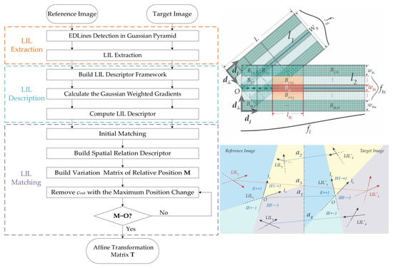
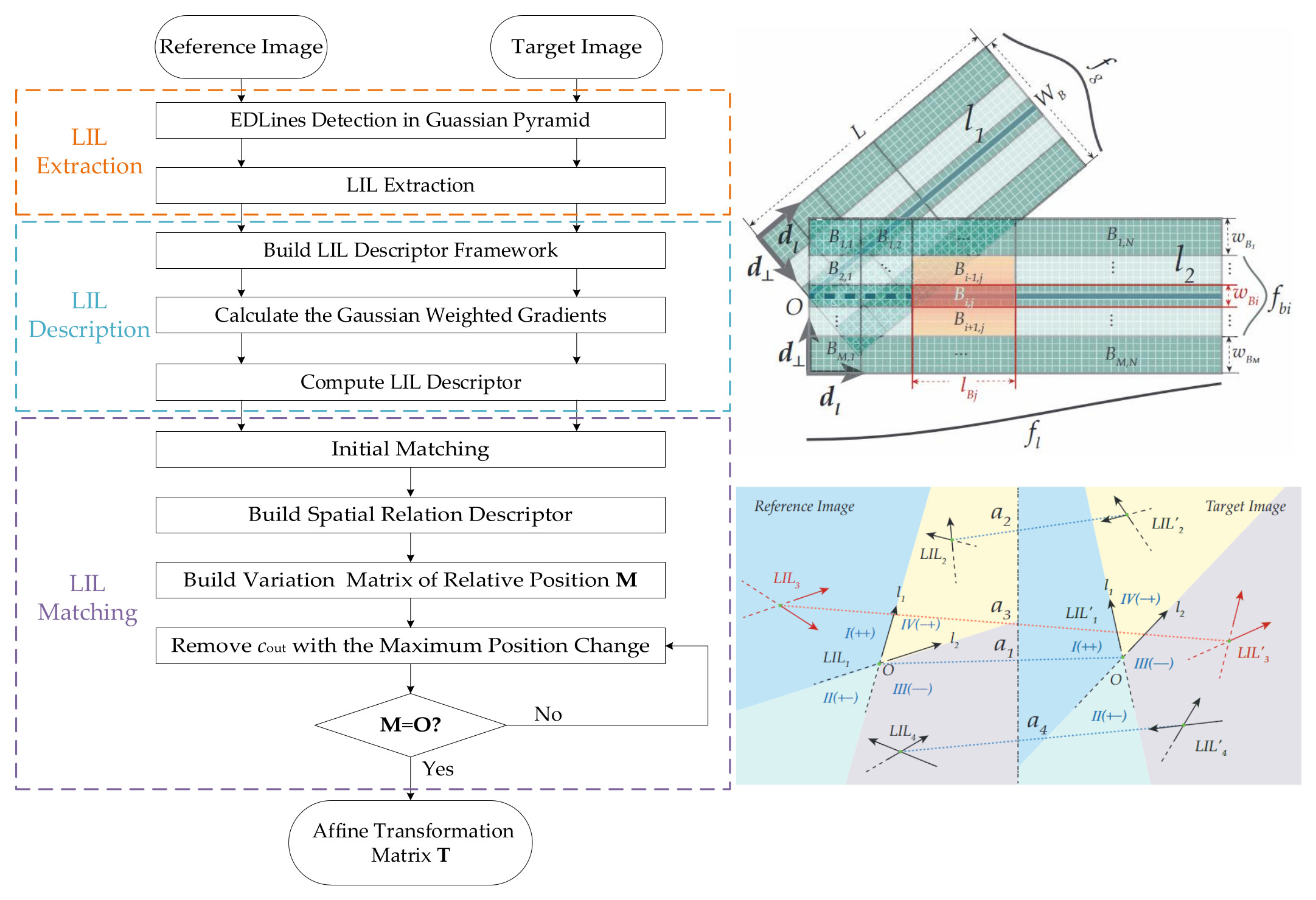
The LIL algorithm can be divided into several main steps: LIL feature extraction, LIL feature description, LIL feature matching, and transformation model estimation. The flowchart is shown in Figure 1.

2.1. LIL Feature Extraction and Description

2.1.1. Multi-scale LIL Feature Extraction

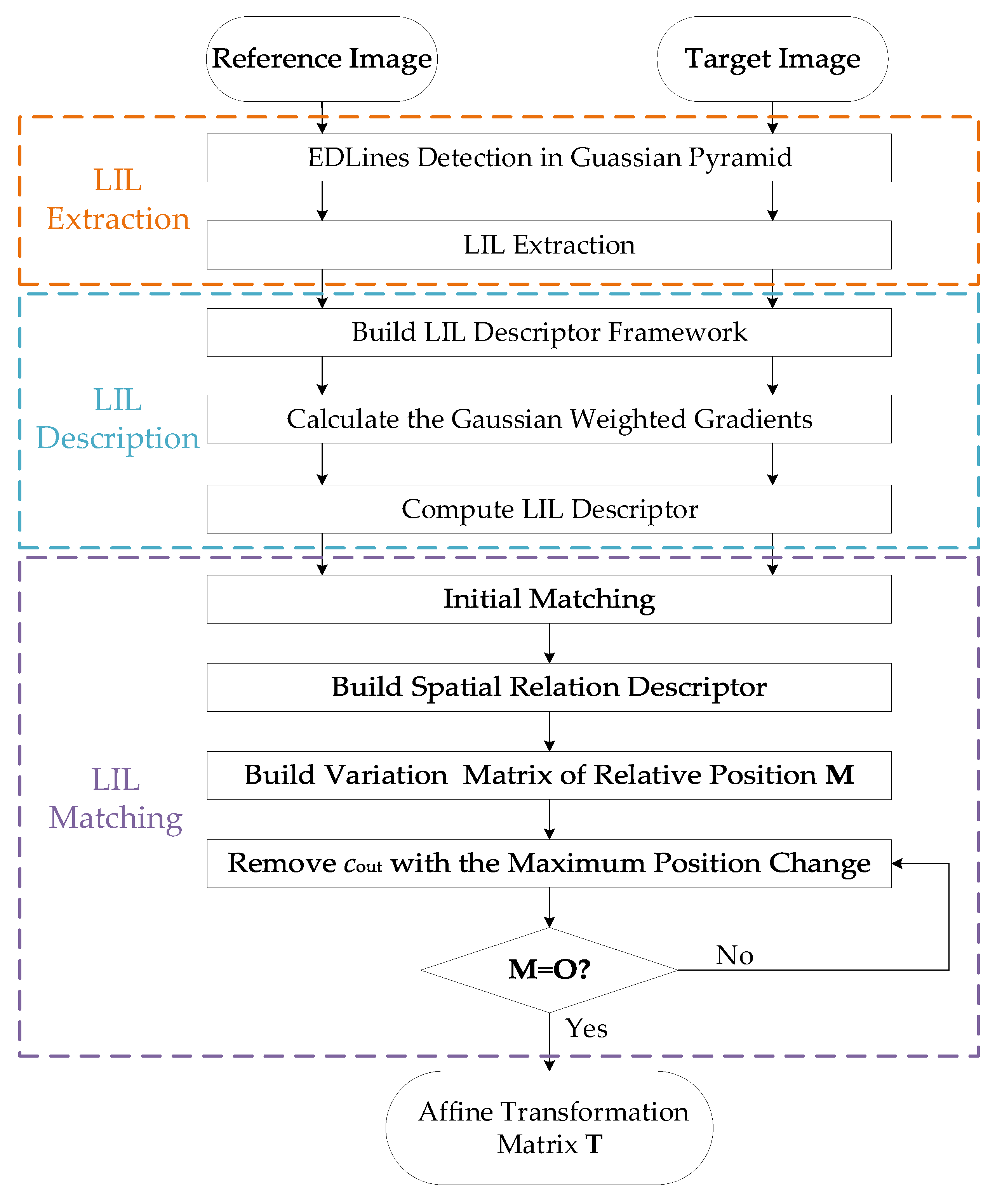
In obtaining intersections, line segments should first be detected. EDLines [15] are used to detect line segments, which can well fit the contours of objects and maintain edge completeness. A Gaussian pyramid is constructed to realize multi-scale feature detection, as shown in Figure 2. A series of layers named octaves is obtained from the original image through Gaussian blur and downsampling; these octaves form an image pyramid with different scales. Given discrepancies between line features and point features, sampling parameters and Gaussian coefficients must be designed.

First, octave number O should be set adaptively according to the image size. For large-scale images, only a few lines will be detected, and their locations will not be highly accurate. As intersections are computed on the basis of line segments, the number and positioning accuracy of intersections will also be affected. For obtaining sufficient and accurate line segments on each octave, with the assumption that the image size is $X\times Y$, the experiment shows that the O should be as follows:

$$O=\lfloor {\log }_2\min (X,Y)-5\rfloor .$$

(1)

In the SIFT, $O=\lfloor {\log }_2\min (X,Y)-2\rfloor$. In this case, only dozens of line segments will be extracted on the octaves with large scales, thereby fewer or none accurate intersections can be detected.

For the same consideration, the Gaussian image is down-sampled by a factor of $\sqrt{2}$ instead of 2 [1]. For an image of size $2000\times 2000$, the octave number is 5, and the size of the fifth octave is $356\times 356$. In this manner, the small number of octaves will not reduce scale invariance, and a large image size can ensure that sufficient line segments are detected on a large-scale image.

The Gaussian coefficients should not be very large; otherwise, the positioning accuracy of line segments will be affected. A large-scale image is generated from a small-scale image as follows:

$$L(x,y,{\sigma }_2)=G(x,y,\sqrt{{\sigma }_2^2-{\sigma }_1^2})\otimes L(x,y,{\sigma }_1),$$

(2)

where $L(x,y,{\sigma }_o)$ is octave o, ${\sigma }_o$ is its scale, and ⊗ is the convolution operation in x and y. The scale varies with the same down-sampling factor, i.e., ${\sigma }_o=\sqrt{2}{\sigma }_{o-1}$. The initial scale ${\sigma }_0$ is set to 0.25.

After the line segments for each octave are detected, the intersections of line segments are calculated to extract LIL. Only line segments on the same octave can form a LIL.

Given the large number of fragmented line segments, line segments and their intersections will be filtered within the following constraints to reduce computation cost and retain accurate features.

• Nearest-neighbor rectangular region search. Search other line segments in a rectangular region centered on line segment $s_i$ to compute intersections, as shown in Figure 3. Define the length of $s_i$ as $S_i$; then, set $b=b_{\mathrm{coef}}·S_i$. The width and length of the rectangular region are $2b$ and $S_i+2b$, respectively. The intersection is reserved when the starting or ending point of $s_j$ is within the rectangular region.
• Intersection angle constraint. The intersection angle of two line segments ${\theta }_i\in [0,{180}^{\circ })$ must satisfy ${\theta }_i>{\theta }_{th}$.
• Distance constraint. The intersection may be on the segment extension line. If it is very far from the line segment, the positioning accuracy will be reduced and the intersection may not make sense; thus, the distance constraint is needed. The distance between $s_i$ and $s_j$ is defined as the distance between the midpoint of shorter line segment $s_{min}=\arg \min \{S_i,S_j\}$ and their intersection, which must meet $d_{ij}>d_{\mathrm{coef}}·S_{min}$.

Obviously, the larger the search range, the more feature points will be detected. However, it will lead to increasing computational cost and decreasing matching precision. The values of $b_{\mathrm{coef}}$, ${\theta }_i$, and $d_{\mathrm{coef}}$ are set empirically. More details are discussed in the Section 3.2.

Figure 3 shows a rectangular region set with $s_1$ as the center. The endpoint of $s_2$ is within the rectangular region, and the intersection angle $\theta$ and distance $d_{12}$ satisfy the constraints of angle and distance. Thus, the intersection O is a valid intersection. However, $s_3$ is not in the rectangular region, $s_4$ does not satisfy the intersection angle constraint, and for $s_5$, $d_{15}$ is too long to meet the distance constraint; none of these lines can form an valid intersection with $s_1$.

The intersections that satisfy the above constraints are selected to build LIL structures. Such structure also need additional information to facilitate the construction of complete LIL features. Mapping all line segments and their intersections detected in each octave to the original image, a LIL feature is $LIL=\{p,\theta ,l_1,l_2,\mathit{LILDes}\}$. p is the intersection coordinate $(x,y)$, and $\theta$ is the intersection angle between two lines. Considering that the intersection of detected EDLines $s_1$ and $s_2$ may lie on the segments or their extension, $l_1$, $l_2$ denote the lines which construct the LIL structure which start from the intersection to one of the endpoints of $s_1$ and $s_2$, whose lengths are $L_1$ and $L_2$, respectively. $\mathit{LILDes}$ is the LIL local feature descriptor, which is described in detail in the next section.

2.1.2. LIL Local Feature Description

The LIL local descriptor is constructed with LIL structures by using the gradients in the LIL neighborhood.

The framework of the LIL descriptor is shown in Figure 4, which is a double-rectangular shape. The descriptor framework consists of two line support regions (LSR), which are centered at lines $l_1$ and $l_2$. The width of each LSR is $W_B$, and the length is equal to that of the center line, i.e., $L_B=L_1$ or $L_2$. Each LSR is divided into M segments along the length direction, N segments along the width direction, i.e., $M\times N$ blocks. The whole LIL contains $2\times M\times N$ blocks, for a total of two LSRs. Figure 4 shows an example where $M=5,N=4$, for a total of 40 blocks. For one LSR, the block of the ith row jth column is denoted as $B_{i,j}$, with a width of $w_{B_i}$ and length of $l_{B_j}$, where $i=1,2,\cdots ,M$, $j=1,2,\cdots ,N$. The width $w_{B_i}$ will be smaller with $B_{i,j}$ closer to the center line. Consequently, the discriminability of descriptors will increase, and features will become increasingly fine near the center line. An example in Figure 4 shows that the corresponding widths of $B_{i,\ast }$ are $\{5,4,3,4,5\}$ pixels, which are determined by empirical values in practice. Similarly, the descriptor is centered on the intersection, so blocks near the intersection should be finer. Therefore, the closer $B_{i,j}$ is to the intersection, the smaller the length $l_{B_j}$. $l_{B_j}$ is determined by the following Formula (3):

$$\begin{array}{c}{l}_{B_j}=\left\{\begin{array}{cc}{l}_0\hfill & j⩽N_0\hfill \\ 2^{N-j-1}{l}_0\hfill & N_0<j⩽N\hfill \end{array}\right.\hfill \\ s.t.\sum _{j=0}^N{l}_{B_j}=L.\hfill \end{array}$$

(3)

where $l_0$ is the minimum length, and $N_0$ is the separation column of different coordinates. When $j>N_0$, $l_{B_j}$ gradually widens, a logarithmic coordinate is adopted. When $j⩽N_0$, an equal-interval coordinate is adopted to prevent the length of $B_{i,0}$ from being very short to be affected by noise. $l_0$ is determined by N and $N_0$. If N and $N_0$ are determined, $l_0$ can be calculated by Equation (3). When $N=4$, and $N_0=2$, the corresponding lengths of $B_{\ast ,j}$ are $\{L/8,L/8,L/4,L/2\}$, as shown in Figure 4.

The gradient $\mathit{g}$ of each pixel is first calculated in the LIL line support region. To achieve rotation invariance, the local coordinate systems of $l_1$ and $l_2$ are built separately, and the pixel gradients are rotated to the local coordinate system. With $l_1$ as an example, the direction along the line segment is denoted as ${\mathit{d}}_l$, and the direction perpendicular to the line pointing to the inner side of LIL is denoted as ${\mathit{d}}_{\perp }$. The origin point is one of vertices of LSR, which lays on the outer side of LIL near the intersection, as shown in Figure 4. $\mathit{g}$ is projected onto this coordinate system ${\mathit{g}}_d={({\mathit{g}}_{{\mathit{d}}_l},{\mathit{g}}_{{\mathit{d}}_{\perp }})}^{\mathrm{T}}$.

To reduce the effect of noise far from LIL on descriptor invariance, gradients are weighted by Gaussian functions to emphasize the gradients close to the center of the descriptor. Pixels closer to the line segment should contribute more to the descriptor, so the first Gaussian weighting function $f_g$ is along direction ${\mathit{d}}_{\perp }$ and centered on the line segment, with ${\sigma }_g$ equal to one half of the width of the LSR, i.e., $f_g=(1/\sqrt{2\pi }{\sigma }_g)e^{-d^2/2{\sigma }_g^2}$, where d stands for the distance between the pixel to the center line. Pixels closer to the intersection should have more contribution. Similarly, along direction ${\mathit{d}}_l$, the Gaussian weighting function $f_l$ is set with the length of LSR as ${\sigma }_l$ and the intersection as the center.

In addition, a local Gaussian weighting function is set for adjacent blocks $B_{i,j}$, $B_{i-1,j}$, and $B_{i+1,j}$ to reduce boundary effects between the block along direction ${\mathit{d}}_{\perp }$. This weighting function is $f_{b_i}=(1/\sqrt{2\pi }{\sigma }_{b_i})e^{-d_k^2/2{\sigma }_{b_i}^2}$, where ${\sigma }_{b_i}=w_{B_i}$, and $d_k$ is the distance between the kth row pixels and the center line of $B_{i,j}$.

Then, the mean and standard deviation of accumulated weighted gradients for each row in each block are used to calculate the LIL descriptor. First, gradients of each row in $B_{i,j}$ and its adjacent blocks are accumulated. In Figure 4, the descriptor of $B_{i,j}$ is computed not only by itself but also by $B_{i-1,j}$ and $B_{i+1,j}$. Classifying the gradients into four directions, the pth row accumulated gradients are as follows:

$$\begin{array}{cc}\hfill u{1}_{ij}\left(p\right)=\lambda \sum _{{\mathit{g}}_{{\mathit{d}}_{\perp }}>0}{f}_l\left(q\right){\mathit{g}}_{{\mathit{d}}_{\perp }},& u{2}_{ij}\left(p\right)=\lambda \sum _{{\mathit{g}}_{{\mathit{d}}_{\perp }}<0}-f_l\left(q\right){\mathit{g}}_{{\mathit{d}}_{\perp }},\hfill \\ \hfill u{3}_{ij}\left(p\right)=\lambda \sum _{{\mathit{g}}_{{\mathit{d}}_l}>0}{f}_l\left(q\right){\mathit{g}}_{{\mathit{d}}_l},& u{4}_{ij}\left(p\right)=\lambda \sum _{{\mathit{g}}_{{\mathit{d}}_l}<0}-f_l\left(q\right){\mathit{g}}_{{\mathit{d}}_l},\hfill \end{array}$$

(4)

where $\lambda =f_g\left(p\right)f_{b_i}\left(p\right)$, and q is the column of the pixel in the block.

The LIL description matrix of $B_{i,j}$, ${\mathbf{LILDM}}_{ij}\in {\mathbb{R}}^{4n}$, can be constructed as follows:

$${\mathbf{LILDM}}_{ij}=\left(\begin{array}{cccc}u{1}_{ij}\left(1\right)& u{1}_{ij}\left(2\right)& \cdots & u{1}_{ij}\left(n\right)\\ u{2}_{ij}\left(1\right)& u{2}_{ij}\left(2\right)& \cdots & u{2}_{ij}\left(n\right)\\ u{3}_{ij}\left(1\right)& u{3}_{ij}\left(2\right)& \cdots & u{3}_{ij}\left(n\right)\\ u{4}_{ij}\left(1\right)& u{4}_{ij}\left(2\right)& \cdots & u{4}_{ij}\left(n\right)\end{array}\right),$$

(5)

where n is the rows of $B_{ij}$ and its adjacent blocks.

The mean and standard deviation of each row in ${\mathbf{LILDM}}_{ij}$ are computed, to form mean vector ${\mathit{M}}_{ij}\in {\mathbb{R}}^4$ and the standard deviation vector ${\mathit{S}}_{ij}\in {\mathbb{R}}^4$. The descriptor of $B_{i,j}$ is ${\mathit{D}}_{ij}$, consisting of ${\mathit{M}}_{ij}$ and ${\mathit{S}}_{ij}$, i.e., ${\mathit{D}}_{ij}={({\mathit{M}}_{ij}^{\mathrm{T}},{\mathit{S}}_{ij}^{\mathrm{T}})}^{\mathrm{T}}\in {\mathbb{R}}^8$. The LIL descriptor is composed of all block descriptors. Two LSRs contain $2MN$ blocks, so $\mathit{LILDes}\in {\mathbb{R}}^{16MN}$ is as follows:

$$\begin{array}{cc}\hfill \mathit{LILDes}& =\{\mathit{D}{1}_{ij}^{\mathrm{T}},\mathit{D}{2}_{ij}^{\mathrm{T}}|i=1,2,\cdots ,M;j=1,2,\cdots ,N\}\hfill \\ & =\{\mathit{M}{1}_{ij}^{\mathrm{T}},\mathit{S}{1}_{ij}^{\mathrm{T}},\mathit{M}{2}_{ij}^{\mathrm{T}},\mathit{S}{2}_{ij}^{\mathrm{T}}|i=1,2,\cdots ,M;j=1,2,\cdots ,N\}.\hfill \end{array}$$

(6)

Finally, the mean vector $\mathit{M}$ and the standard deviation vector $\mathit{S}$ are normalized separately because of different magnitudes. Each element in the vector is normalized to [0, 1]. In addition, the element in the descriptor should not exceed the light threshold to resist nonlinear illumination. The threshold is generally set to 0.4 [17]. However, we divide the LSR along direction ${\mathit{d}}_l$ and the values of ${\mathit{D}}_{ij}$ calculated in different blocks is proportional to the block lengths, thereby the light threshold is set to $0.4l_{B_i}/L$.

2.2. LIL Matching

The preliminary LIL matching is achieved by comparing the Euclidean distance between LIL local descriptors, but brute force matching is time consuming and less robust. Therefore, given the feature of LIL structures, the matching pairs are preliminarily selected on the basis of the intersection angle and length ratio of LIL. On one hand, for satellite remote sensing images, the difference of the same intersection angle in the two images should not be more than ${30}^{\circ }$ [27], i.e., $|{\theta }_i-{\theta }_i^{\prime }|⩽{30}^{\circ }$. On the other hand, for the same LIL, the change in the ratio of lengths between two line segments will not be very large. Set $L_{\mathrm{ratio}}=L_1/(L_1+L_2)$, so the corresponding LILs should satisfy $|L_{{\mathrm{ratio}}_i}-L_{{\mathrm{ratio}}_i}^{\prime }|⩽0.2$. Then, after brute force matching and a symmetry test, the initial matching set can be obtained as $\mathcal{IMP}=\left\{(LI{L}_i,LI{L}_i^{\prime })\right|i=1,2,\cdots ,N_I\}$.

However, many false matches exist in the initial matching set. We design an outlier removal strategy based on the LIL structure and spatial relative relation. We construct a spatial relation descriptor and variation matrix of relative position based on affine properties and graph matching to eliminate outliers step by step.

It’s worth noting that the LIL matching method is restricted to satellite remote sensing images. Images acquired by orbital systems satisfy the plane hypothesis. The satellite orbit has high attitude so that we can ignore the elevation error of the ground. On this basis, the registration model can be considered as affine transformation and the spatial relation descriptor is also designed based on affine properties.

2.2.1. LIL Spatial Relation Descriptor

The spatial relations between outliers and inliers are always wrong. According to the LIL structure and geometric relations, we construct a spatial relation descriptor, which can record the variations in relative positions between any of matches and is used to construct the variation matrix of relative position.

The relationship between two satellite remote sensing images can be regarded as affine transformation. Affine transformation has the following properties. (1) Points on a line still lie on the same line after affine transformation; (2) Points on one side of a line are still on the same side of the same line after affine transformation. According to the two properties and the LIL structure, the LIL spatial relation descriptor can be constructed.

LIL divides the image into four parts, and the LIL local coordinate system is defined with the intersection O as origin, and $l_1$ and $l_2$ as coordinate axises, as shown in Figure 5. The left side and the positive half of coordinate axis are defined as positive, whereas the right side and the negative half of that are negative, constituting four quadrants $\left\{I\right(++),II(+-),III(--),IV(-+\left)\right\}$. For any two LIL matches in $\mathcal{IMP}$, $a=(LI{L}_i,LI{L}_i^{\prime })$ and $b=(LI{L}_j,LI{L}_j^{\prime })$, the quadrant of $LI{L}_j$ in $LI{L}_i$ coordinate system on the reference image is calculated, i.e., $Q(a,b)=\left\{q\right|q=1,2,3,4,a\ne b;q=0,a=b\}$. Similarly, the quadrant of $LI{L}_j^{\prime }$ in the $LI{L}_i^{\prime }$ coordinate system $Q^{\prime }(a,b)$ can be obtained on the target image. As shown in Figure 5, for match $a_3$ under the local coordinate system of match $a_1$, $Q(a_1,a_3)=1$, $Q^{\prime }(a_1,a_3)=3$; instead, for $a_1$ under the $a_3$ coordinate system, $Q(a_3,a_1)=3$, $Q^{\prime }(a_3,a_1)=1$.

The spatial relation descriptor $\psi (a,b)$ is computed as follows:

$$\psi (a,b)=\left\{\begin{array}{cc}0\hfill & Q(a,b)=Q^{\prime }(a,b)\hfill \\ 1\hfill & |Q(a,b)-Q^{\prime }(a,b)|=1||3\hfill \\ 2\hfill & |Q(a,b)-Q^{\prime }(a,b)|=2\hfill \end{array}\right.,a,b\in \mathcal{IMP}.$$

(7)

According to the definition, the spatial relation descriptor of one match is the number of quadrants that change from the reference image to the target image in the coordinate system of another match. If the quadrant remains unchanged, then the descriptor value is 0; otherwise, the value is 1 or 2 with quadrant changing.

The spatial relation descriptor reflects the relative variation in spatial relation between LIL matches. For one LIL match a, the more matches change relative to its position, the more non-zero descriptors, i.e., $\psi (a,\ast )\ne 0$. By contrast, the more non-zero descriptors are present, i.e., $\psi (\ast ,a)\ne 0$, the greater the position of a changes relative to others. Therefore, a is likely to be an outlier in the aspect of geometric relation. A matching set with no outlier in spatial relation should satisfy the following:

$$\sum _{a,b\in \mathcal{IMP}}\psi (a,b)=0.$$

(8)

That means the relative positions between any of LIL matches remain unchanged.

Figure 5 shows four 4 LIL matches, where $a_1,a_2,a_4$ are inliers, and $a_3$ is outlier. Obviously, $\psi (a,b)=0,a,b\in \{a_1,a_2,a_4\}$. For matches $a_1$ and $a_3$, the spatial relation descriptor can be computed as $\psi (a_1,a_3)=|Q(a_1,a_3)-Q^{\prime }(a_1,a_3)|=|1-3|=2$; by contrast, $\psi (a_3,a_1)=2$ in the coordinate system of $a_3$. Similarly, the relations between $a_2$, $a_4$, and $a_3$ can be judged to calculate descriptors.

2.2.2. LIL Outlier Removal Based on LIL Spatial Relation Descriptor and Graph Theory

LIL spatial relation descriptors record the variations in relative positions between two matches. According to the theory of graph matching [34], a variation matrix of relative position $\mathbf{M}\in {\mathbb{R}}^{N_I\times N_I}$ can be constructed, and its elements are computed with the spatial relation descriptor:    

$$\begin{array}{c}M(a,b)=\psi (a,b)+\psi (b,a),\hfill \\ M(a,b)=M(b,a).\hfill \end{array}$$

(9)

$\mathbf{M}$ is a non-negative, symmetric matrix. Matches in $\mathcal{IMP}$ can be considered the nodes of an undirected graph, whereas any pair of matches constitutes graph edges. The diagonal elements $M(a,a)=0$, whereas $M(a,b)$ are weights for edges, which represent the variation degree of relative positions between a and b. The larger the value of $M(a,b)$ is, the greater the variation of relative positions between matches. When $M(a,b)=0$, the relative positions between them do not change. If the position of b changes relative to a while a stays unchanged against b, then $M(a,b)=\psi (a,b)$. If both their positions vary relative to each other, then the value of $M(a,b)$ will be greater.

With Figure 5 as an example, after spatial relation descriptors are calculated, the elements in the matrix can be computed, such as $M(a_1,a_3)=M(a_3,a_1)=\psi (a_1,a_3)+\psi (a_3,a_1)=2+2=4$. The variation matrix of relative position can be obtained as follows:

$$\mathbf{M}=\left(\begin{array}{cccc}0& 0& 4& 0\\ 0& 0& 1& 0\\ 4& 1& 0& 1\\ 0& 0& 1& 0\end{array}\right).$$

(10)

Mark matches in $\mathcal{IMP}$ in indicator vector $\mathit{x}$ of $N_I$ dimensions, such that $x\left(a\right)=1$ if a is an inlier and $x\left(a\right)=0$ otherwise. The score of total variation of spatial positions in the matching set is as follows:

$$S=\sum _{a,b\in \mathcal{IMP}}M(a,b)={\mathit{x}}^{\mathrm{T}}\mathbf{M}\mathit{x}.$$

(11)

The problem of eliminating outliers is finding the optimal solution ${\mathit{x}}^{\ast }$, which minimizes the score S, i.e., ${\mathit{x}}^{\ast }=\arg \min \left({\mathit{x}}^{\mathrm{T}}\mathbf{M}\mathit{x}\right)$. On account of the positive semi-definite variation matrix of relative position $\mathbf{M}$ and the fact that the relative positions between inliers obtained in the final solution should not change, the following holds:

$${\mathit{x}}^{\ast }{}^{\mathrm{T}}\mathbf{M}{\mathit{x}}^{\ast }=0.$$

(12)

Divide $\mathcal{IMP}$ into two sets: clean matching set $\mathcal{CMP}$ and removed matching set $\mathcal{RMP}$. Correspondingly, ${\mathit{x}}^{\ast }=({\mathit{x}}_C,{\mathit{x}}_R)$, where ${\mathit{x}}_R=\mathbf{0}$, then Equation (12) can be decomposed into the following:

$$({\mathit{x}}_C^{\mathrm{T}},{\mathit{x}}_R^{\mathrm{T}})\left(\begin{array}{cc}{\mathbf{M}}_C& \mathbf{B}\\ {\mathbf{B}}^{\mathrm{T}}& {\mathbf{M}}_R\end{array}\right)\left(\begin{array}{c}{\mathit{x}}_C\\ {\mathit{x}}_R\end{array}\right)={\mathit{x}}_C{}^{\mathrm{T}}{\mathbf{M}}_C{\mathit{x}}_C=0,$$

(13)

where ${\mathbf{M}}_C$ and ${\mathbf{M}}_R$ are the matrixes associated with inliers and outliers respectively. Because ${\mathit{x}}_C\left(a\right)=1$, the following holds:

$${\mathbf{M}}_C=\mathbf{O}.$$

(14)

Therefore, a strategy should be designed to remove outliers from $\mathcal{IMP}$ such that ${\mathbf{M}}_C=\mathbf{O}$. Finally, we can obtain $\mathcal{CMP}$ with $N_C$ matches and $\mathcal{RMP}$ with $N_R$ matches, where $N_C+N_R=N_I$.

A greedy algorithm is adopted to remove outliers successively until $\mathbf{M}=\mathbf{O}$. To reduce computational complexity, the row and column in $\mathbf{M}$ corresponding to the removed match are deleted, and the matrix dimension can gradually be reduced [34]. The algorithm steps are as follows.

• Initialize $\mathit{x}$ with the $N_I\times 1$ unity vector, and $\mathcal{RMP}=⌀$.
• Compute the accumulated error and solve the match with the maximum error. The accumulated error of each match is obtained by summing each row of the variation matrix of relative position, and the matches corresponding to the maximum value can be solved as follows:

  $$\mathcal{OMP}=\underset{a\in \mathcal{IMP}}{\arg \max }\sum _{b\in \mathcal{IMP}}M(a,b),$$

  (15)

  where $\mathcal{OMP}$ is the set of candidate removed matches. If $\mathcal{OMP}=⌀$, then return ${\mathit{x}}^{\ast }=\mathit{x}$; otherwise, set $N_o=Card\left(\mathcal{OMP}\right)$. More than one match may correspond to the maximum accumulated error. If $N_o=1$, then the outlier is $a\in \mathcal{OMP}$; otherwise, these candidate matches should be compared by the number of matches whose position changes relative to them.

  $$c_{out}=\left\{\begin{array}{cc}a\in \mathcal{OMP}\hfill & N_o=1\hfill \\ \underset{a\in \mathcal{OMP}}{\arg \max }{\displaystyle \sum _{b\in \mathcal{IMP}}}M(a,b)\oplus 0\hfill & N_o>1\hfill \end{array}\right.,$$

  (16)

  where ⊕ is the xor symbol used to count the number of non-zero elements in the row corresponding to LIL match a.
• Remove match $c_{out}$, and add it to $\mathcal{RMP}$. Delete the row and column in $\mathbf{M}$ corresponding to $c_{out}$, and set $\mathit{x}\left(c_{out}\right)=0$.
• Repeat Steps (2)and (3), until $\mathbf{M}=\mathbf{O}\in {\mathbb{R}}^{N_C\times N_C}$. Return ${\mathit{x}}^{\ast }=\mathit{x}$, and add matches such that ${\mathit{x}}^{\ast }\left(a\right)=1$ to $\mathcal{CMP}$.

All matches with large variations in spatial relation are eventually eliminated. By using all matches in $\mathcal{CMP}$, we can estimate the affine transformation matrix $\mathbf{T}$ with the least squares method. To obtain high-accuracy transformation model, we further remove matches with large registration errors and recalculate the final transformation model $\mathbf{T}$.

For Figure 5, the variation matrix of relative position $\mathbf{M}$ is shown as Equation (10). Each row is summed to obtain $\{4,1,6,1\}$; then, $c_{out}=\arg \max \{4,1,6,1\}=a_3$. Remove $a_3$, then $\mathbf{M}=\mathbf{O}\in {\mathbb{R}}^{3\times 3}$, thereby removing outliers. The pseudocode of LIL outlier removal is shown in Algorithm 1.

Algorithm 1 LIL Outlier Removal.

Input:$\mathcal{IMP}=\left\{(LI{L}_i,LI{L}_i^{\prime })\right\}$ of size $N_I$. Output:$\mathit{x}$ of size $N_I$,$\mathcal{CMP}$ of size $N_C$, $\mathcal{RMP}$ of size $N_R$, $N_I=N_C+N_R$ 1: for$a,b\in \mathcal{IMP}$do 2:     Calculate $Q(a,b)$, $Q^{\prime }(a,b)$ 3:     Calculate spatial relation descriptor $\psi (a,b)$ by Equation (7) 4: Build variation matrix of relative position $\mathbf{M}$ by Equation (9) 5: Initialize $\mathit{x}$ and $\mathcal{RMP}$ 6: while$\mathbf{M}\ne \mathbf{O}$do 7:     Calculate candidite removed matches $\mathcal{OMP}\leftarrow \underset{a\in \mathcal{IMP}}{\arg \max }{\displaystyle \sum _{b\in \mathcal{IMP}}}M(a,b)$ 8:     if $N_O=0$ then 9:         return ${\mathit{x}}^{\ast }\leftarrow \mathit{x}$, $\mathcal{CMP}\leftarrow {\mathcal{IMP}}^{\ast }$ and $\mathcal{RMP}$ 10:     else 11:         if $N_O>1$ then 12:            $c_{out}\leftarrow a\in \mathcal{OMP}$ 13:         else 14:            $c_{out}\leftarrow \underset{a\in \mathcal{OMP}}{\arg \max }{\displaystyle \sum _{b\in \mathcal{IMP}}}M(a,b)\oplus 0$ 15:     Remove $c_{out}$ and add it to $\mathcal{RMP}$ 16:     Update $\mathbf{M}$, $x\left(c_{out}\right)\leftarrow 0$ 17: return${\mathit{x}}^{\ast }\leftarrow \mathit{x}$, $\mathcal{CMP}\leftarrow {\mathcal{IMP}}^{\ast }$ and $\mathcal{RMP}$

3. Experiment and Results

The proposed algorithm is tested on images with simulated transformations and real multi-temporal remote sensing images of urban scenes. The results are compared with those of similar and state-of-the-art algorithms under reasonable accuracy evaluation. To evaluate the LIL local descriptor and the LIL outlier removal method, we compare them with the SIFT descriptor and RANSAC, respectively.

3.1. Accuracy Evaluation

For general feature-based remote sensing image registration, the accuracy indexes usually include the root mean squared error (RMSE) of projected distance and precision, which are as follows:

$$RMSE=\frac{1}{N}\sqrt{{\sum }_i{[\mathbf{T}\left(p_i\right)-{\mathbf{T}}_0\left(p_i\right)]}^2},$$

(17)

$$Precision=\frac{CN}{CN+FN},$$

(18)

where ${\mathbf{T}}_0$ is the ground truth affine model, $p_i$ is the coordinate of the sampled point, and $CN$ and $FN$ denote the number of correct and false matches, respectively, in the final matching set of number $TN$. The matches with projected distance <3 [28] are regarded as correct matches in this study.

In addition, to evaluate the LIL outlier removal method, we use the following indicators:

$$Accuracy=\frac{CN+DF}{CN+DF+FN+DC},$$

(19)

$$Recall=\frac{CN}{CN+DC},$$

(20)

$$Specificity=\frac{DF}{DF+FN},$$

(21)

where $DF$ and $DC$ denote the number of deleted false/correct matches, respectively. $Accuracy$ can measure the closeness of identified matches to the actual matches. $Recall$ represents the ratio of correct matches, which are identified in accordance with the actual situation. $Specificity$ represents the ratio of false matches that are identified correctly.

3.2. Parameter Setting

Some parameters are determined by experiments in the process of LIL feature extraction and description, as shown in the following

Table 1. Parameter setting.

Notation	Parameter	Default Value
$b_{coef}$	Coefficient of search range	0.5
${\theta }_{th}$	Threshold of intersection angle constraint	${30}^{\circ }$
$d_{coef}$	Coefficient of distance constraint	5
M	Number of rows of blocks in LSR	9
$\{w_{B_1},w_{B_2},\cdots ,w_{B_9}\}$	Widths of blocks	$\{11,9,7,6,5,6,7,9,11\}$
N	Number of columns of blocks in LSR	4
$N_0$	Separation column of coordinates	2
$16MN$	Dimension of LIL local descriptor	576

.

In Table 1, $b_{coef}$, ${\theta }_{th}$, and $d_{coef}$ are used for intersection detection and filtering. If the values of $b_{coef}$ and $d_{coef}$ are very large or ${\theta }_{th}$ is very small, then the locations of the detected intersections will be inaccurate; otherwise, they lead to insufficient features. The values in the table are set by multiple experiments. For example, the proposed algorithm was tested on four pairs of real images with $\{b_{coef},{\theta }_{th},d_{coef}\}=\{0.5,{30}^{\circ },5\}$, and the total number of correct matches, average precision (without LIL outlier removal) and $RMSE$ are 639, 31.04%, and 0.64, respectively. However, when the parameters are $\{0.3,{40}^{\circ },3\}$, the results are 312, 29.36%, and 1.12, respectively. Insufficient correct matches lead to inaccurate result. In contrast, the results are 996, 28.48%, and 0.90 with constraint parameters $\{0.7,{20}^{\circ },7\}$. More correct matches do not increase the precision and registration accuracy but result in more time spent in describing and matching.

For LIL local description, the widths of blocks ${\mathit{w}}_B=\{w_{B_1},w_{B_2},\cdots ,w_{B_9}\}$ and the number of rows M are determined by experiments. If the blocks are very wide or numerous, then the descriptor is not sufficiently fine for achieving high accuracy, and pixels very far from LIL have minimal significance in description. On the contrary, the robustness of LIL descriptors with large local distortions will be reduced. $M=9$ is a proper value according to [17,28]. Several combinations are tested on twenty-four pairs of real remote sensing images, and the average results are depicted in

Table 2. Experimental Results with different parameters (M, ${\mathit{w}}_B$).

Parameter Setting ($\mathit{N}=4$)	Total Correct Matches	Precision (%)	Descriptor Dimension
M = 7, ${\mathit{w}}_B=\{7,6,5,3,5,6,7\}$	8106	84.30	448
M = 7, ${\mathit{w}}_B=\{9,8,7,5,7,8,9\}$	7716	84.96	448
M = 7, ${\mathit{w}}_B=\{11,9,7,5,7,9,11\}$	7605	84.82	448
M = 9, ${\mathit{w}}_B=\{7,6,5,4,3,4,5,6,7\}$	7992	84.61	576
M = 9, ${\mathit{w}}_B=\{9,8,7,5,3,5,7,8,9\}$	7883	84.66	576
M = 9, ${\mathit{w}}_B=\{11,9,7,6,5,6,7,9,11\}$	8483	85.39	576
M = 11, ${\mathit{w}}_B=\{11,9,8,7,5,3,5,7,8,9,11\}$	8352	85.53	704
M = 11, ${\mathit{w}}_B=\{11,10,9,7,6,5,6,7,9,10,11\}$	7687	85.03	704

. To balance the accuracy and dimension, ${\mathit{w}}_B=\{11,9,7,6,5,6,7,9,11\}$ is set.

The selection of the number of columns N is based on the same consideration.

Table 3. Experimental Results with different parameters ($N,N_0$).

Parameter Setting		Total Correct Matches	Precision (%)
N = 4	$N_0$ = 1	8017	83.23
	$N_0$ = 2	8483	85.39
	$N_0$ = 3	8247	84.60
	$N_0$ = 4	8337	85.09
N = 3	$N_0$ = 1	7726	83.64
	$N_0$ = 2	8083	84.74
	$N_0$ = 3	8058	84.53

shows the average results of several combinations of N and $N_0$. In this study, N is set to 4 to balance the dimensions and discriminability of descriptors. Besides, experiments show that $N_0=2$ can maximize the number of correct matches when $N=4$.

The dimension of LIL local descriptor is 576, which is eight times that of LBD and RLI in consequence of two LSRs and division along the direction of the line segment. Although the dimension is relatively high, it is much finer and more robust without excessively increasing the computation load for matching.

3.3. Experimental Results on Images with Simulated Transformations

Experiments are conducted on images with simulated transformations, and the proposed algorithm is compared with several similar state-of-the-art algorithms, including SIFT [1], LP [24], MSLD [16], RLI [28], and LJL [27]. SIFT is the most widely used algorithm for image matching. LP and MSLD are the representatives of line matching algorithms. LP uses an affine invariant derived from one line and two coplanar points to calculate the similarity of two line segments. The combination of line and point is similar to the proposed method. MSLD is based on the appearance of the pixel support region. Many line descriptors are inspired by MSLD, such as SMSLD, LBD and RLI. RLI matches line descriptor first and then selects triplets of intersections of matching lines to estimate affine transformation iteratively. The LJL structure uses two line segments and their intersecting junction for constructing circular descriptors and propagation matching strategies, and the left line segments are matched by utilizing the local homographies estimated from their neighboring matched LJLs. Both RLI and LJL use intersections as matching points which are smilar to the proposed method. In the experiments, we used midpoints of line segments of LP and MSLD and intersections of RLI and LJL as matching points to estimate the affine transformation model by RANSAC.

The original image was taken by the WorldView-1 satellite on October 5, 2007 over Addis Ababa, Ethiopia, with a ground sample distance (GSD) of 0.46 m, as shown in Figure 6. A series of transformations is then performed on the image to verify the robustness of the LIL algorithm against scale, rotation, illumination variations, and cloud cover.

3.3.1. Comparison of Matching Results with Different Methods

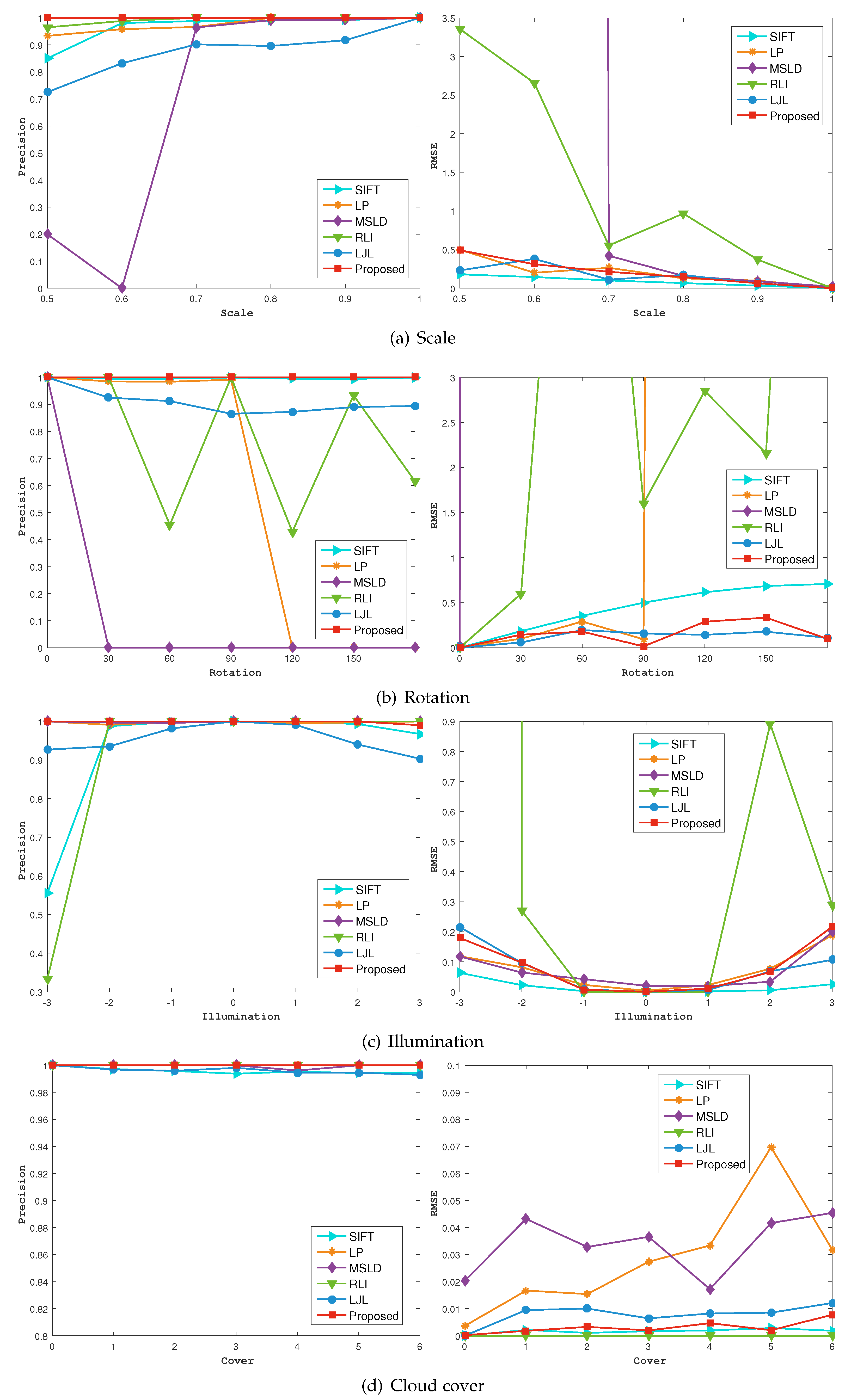
Figure 7 shows the $Precision$ and $RMSE$ of the different algorithms tested on simulated images. The scale ratio ranges from 1 to 0.5, and the rotation angle is in the range of $[0^{\circ },{180}^{\circ }]$. Illumination variations are simulated by increasing or decreasing the image intensity. In Figure 7c, negative coordinates indicate dark illumination, and positive coordinates indicate bright illumination. Regarding occlusion, cloud patches are extracted from a real remote sensing image with cloud cover (with gray value 230∼255), which are added randomly to the test image with the number of patches varying from 8 to 20.

The data in Figure 7 show that the $Precision$ and $RMSE$ of the LIL can reach nearly 100% precision and sub-pixel accuracy, respectively, under the conditions of scale, rotation, illumination variations, and cloud cover. MSLD performs the worst under scale and rotation transformation. MSLD cannot achieve registration given considerable scale changes, and it has almost no rotation invariance. LP keeps rotation invariance in $0^{\circ }$∼${90}^{\circ }$. The $RMSE$ of RLI can reach ${\mathrm{e}}^{-13}$ given sufficient matches, as shown in Figure 7d. However, it loses robustness with rotation variations or dark lighting conditions, and its overall accuracy is lower than the others’. SIFT, LJL and the proposed algorithm remain robust in these experiments. Except for relatively high $RMSE$ in the case of large rotation angle, SIFT can acheive higher registration accuracy than LIL because of numerous detected points. The $RMSE$ of LJL under extreme conditions is sometimes slightly higher than that of the proposed algorithm, with its $Precision$ lower than ours at the same time. All of these algorithms have good robustness against occlusion, but the registration accuracies of LP and MSLD algorithms are relatively low.

3.3.2. Comparison of SIFT and LIL Descriptor

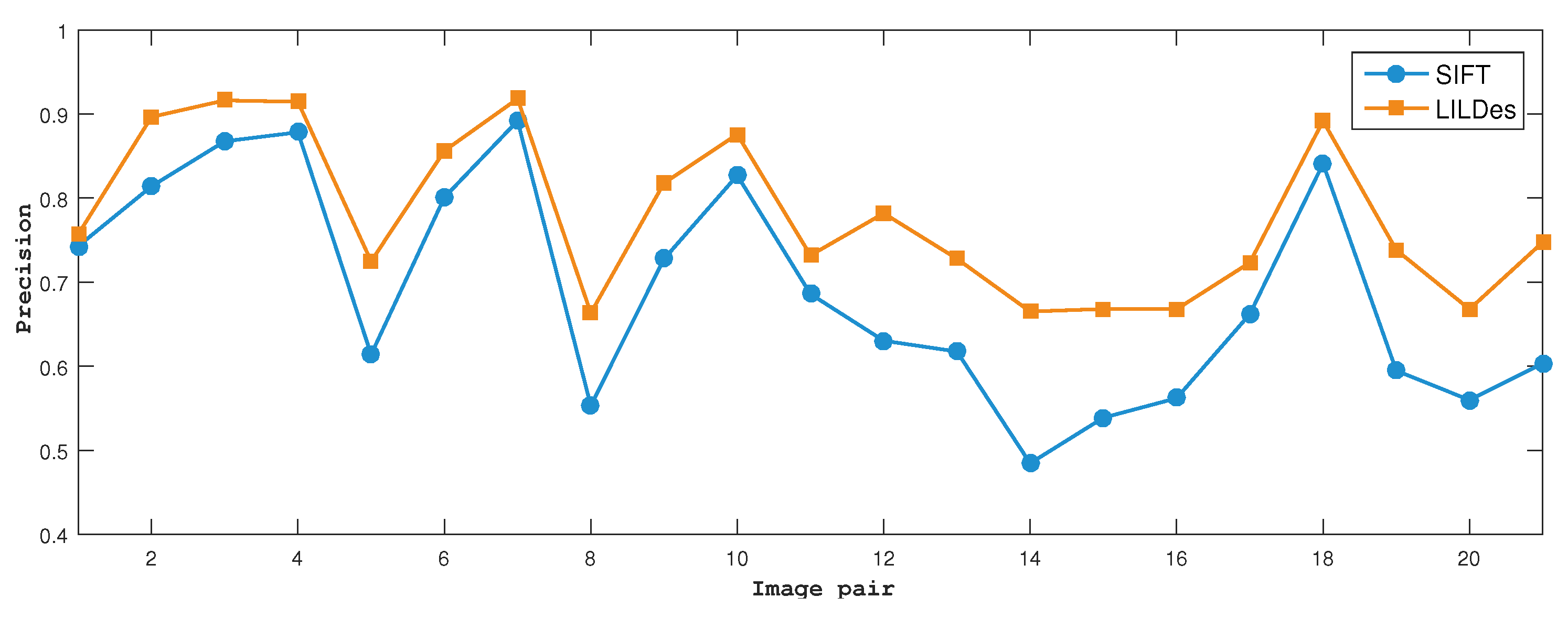
In order to validate the superiority of the LIL local descriptor, this study compares it with the SIFT descriptor on simulated images with large background variations which are different combinations of scale, rotation, illumination, and occlusion variations. Feature points are intersections extracted by the LIL detection in all experiments, and are described by SIFT and LIL descriptors, respectively. Figure 8 shows the precisions after brute force matching. Overall, the precisions of matching results using the LIL descriptor are 3% 18% higher than those using the SIFT descriptors, which proves that the LIL descriptor have higher discriminability for the same feature points. Especially for low-precision test results, the advantage of the LIL descriptor is more obvious.

3.4. Experimental Results on Real Multi-Temporal Remote Sensing Images

Multi-temporal remote sensing images of urban areas with different types of large background variations are selected for testing to validate the robustness of the proposed algorithm in real situations. The datasets are shown in

Table 4. Datasets of real remote sensing images.

No.	Type	Location	Source	Date (yyyy/mm/dd)	Size	GSD
1	Years	Anqing, China	GoogleEarth	2009/12/06	922*865	4 m
			GoogleEarth	2016/12/05	922*863	4 m
2	Hurricane	Seaside Heights, America	GeoEye-1	2010/09/07	1190*994	0.5 m
			GeoEye-1	2012/10/31	1170*1002	0.5 m
3	Flooding	Nowshera, Pakistan	Quickbird	2010/08/05	1888*1896	2 m
			Quickbird	2010/08/05	1888*1896	2 m
4	Seasons	Huhhot, China	GoogleEarth	2017/01/20	1076*829	2 m
			GoogleEarth	2018/06/30	1076*829	2 m
5	Earthquake	Port-Au-Prince, Haiti	GeoEye-1	2010/01/13	2504*1884	0.5 m
			IKONOS	2008/09/29	1240*952	0.82 m
6	Tornado	Yazoo City, America	Quickbird	2010/04/28	3432*2664	0.6 m
			Quickbird	2010/03/23	2992*2380	0.6 m

.

The datasets include images captured in different years or seasons and high-resolution remote sensing images taken before and after natural disasters, which introduce great challenges for robust and high-accuracy registration.

Table 5. Comparison of registration results on real remote sensing images.

Algorithm	Evaluation	1	2	3	4	5	6
SIFT	TN	170	112	140	82	283	25
	CN	97	8	32	3	3	0
	Precision (%)	57.1	7.1	22.5	3.6	1.1	0
	RMSE	8.63	26.91	41.72	—	—	—
LP	TN	7	48	20	4	4	1
	CN	3	29	11	0	0	0
	Precision (%)	42.9	60.4	55.0	0	0	0
	RMSE	81.52	6.47	5.53	—	—	—
MSLD	TN	6	8	20	5	1	11
	CN	3	5	10	0	0	9
	Precision (%)	50	62.5	0	0	0	81.8
	RMSE	15.42	5.89	23.41	—	—	—
RLI	TN	25	4	70	0	0	6
	CN	17	2	70	0	0	0
	Precision (%)	68	25	100	0	0	0
	RMSE	12.86	92.21	0.57	—	—	20.90
LJL	TN	331	2669	365	34	837	544
	CN	215	1194	241	7	478	377
	Precision (%)	65.0	44.7	66.0	20.6	57.1	69.3
	RMSE	2.48	0.97	1.30	98.75	1.30	6.15
Proposed	TN	14	190	320	19	21	30
	CN	14	190	320	19	20	29
	Precision (%)	100	100	100	100	95.2	99.2
	RMSE	0.80	0.60	0.45	0.69	1.17	0.99

shows the registration results of different algorithms on the six image pairs.

The table shows that SIFT, LP, MSLD, and RLI have relatively poor performance. Although SIFT achieves high accuracy on simulated images, it performs poorly on real images with large variations. Many SIFT points are detected, but fail to match correctly using descriptors that can not resist large background variations. LP and MSLD are not satisfactory in terms of matching numbers and $Precision$. For image pair 4–6, the above methods are completely unable to achieve registration, and RLI diverges in the iterative process. LJL detects the most features and has good robustness, but its $Precision$ is not high. Numerous false matches result in relatively large $RMSE$. The proposed algorithm is the most robust and accurate among the compared methods. Although detected matching numbers are not large, the $Precision$ can reach almost 100% on these image pairs, and registration accuracy reaches sub-pixel level.

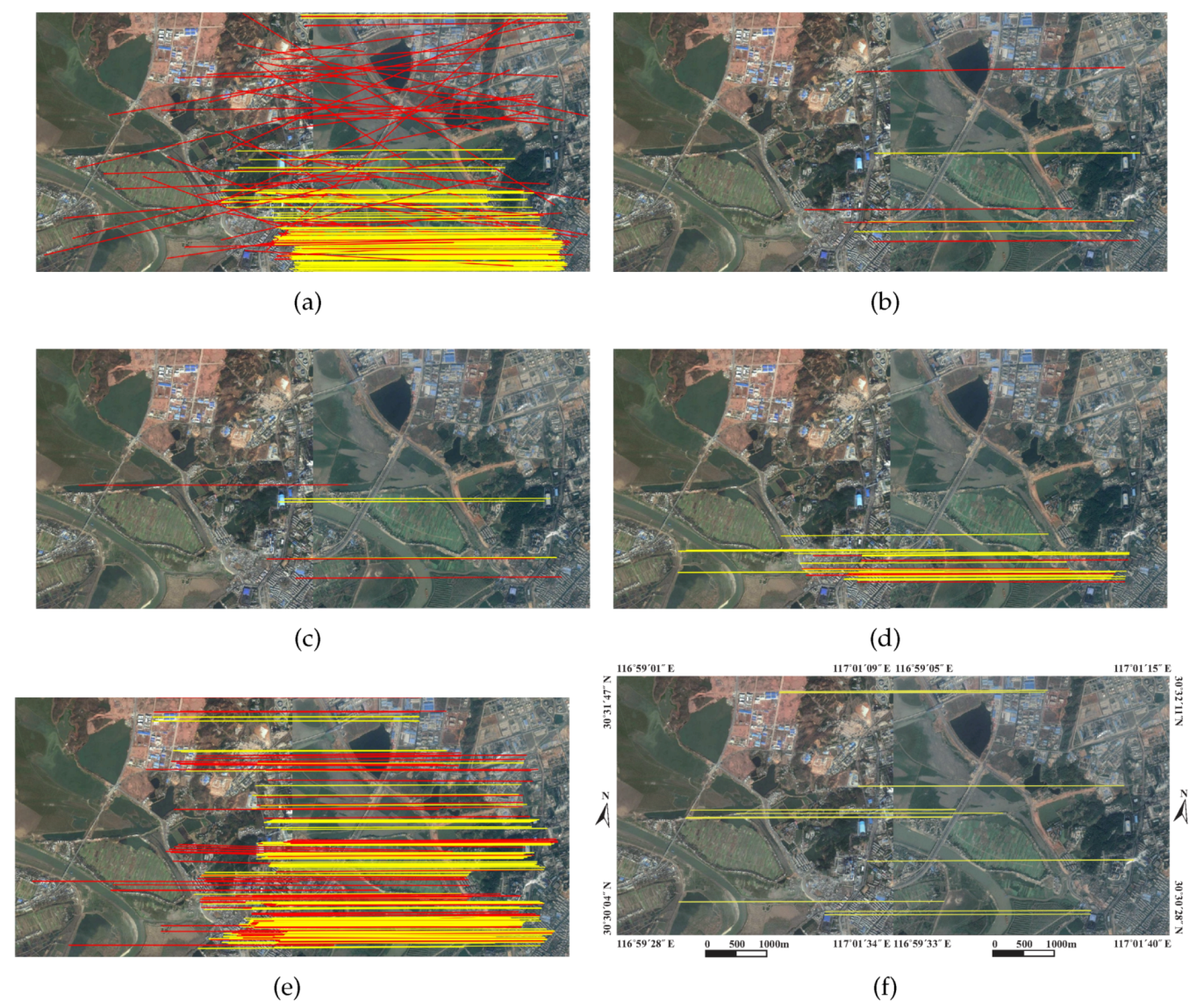
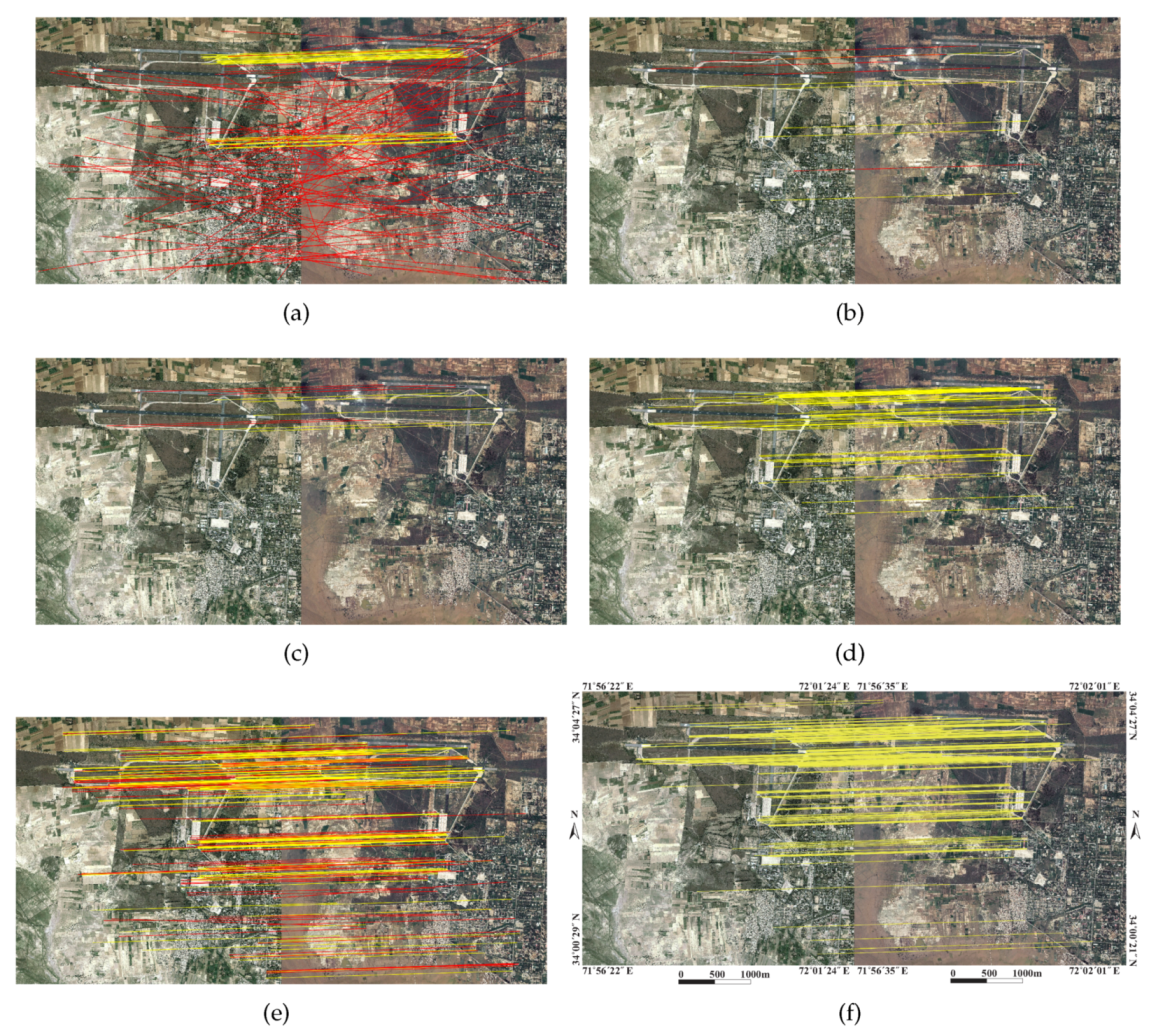
Figure 9, Figure 10, Figure 11, Figure 12, Figure 13 and Figure 14 illustrate the matching results of these algorithms. The yellow and red lines indicate correct and false matches, respectively. Figure 9 shows a comparison of matching results for image pair 1. Bridges and buildings undergo great changes over time. Figure 9a shows that many false matches which do not conform to the spatial relations are detected by SIFT. As shown in Figure 9b–d, the matches detected by LP, MSLD and RLI are low in quantity, distributed unevenly, and have many outliers, so they cannot realize correct registration. Although LJL detects numerous matches, as shown in Figure 9e, the final matches are clustered on the right side of the image because the bridge on the left side changes greatly and has few features. Consequently, the registration accuracy of LJL is relatively low. The matching intersections detected by the proposed algorithm are uniformly distributed, so higher accuracy can be obtained.

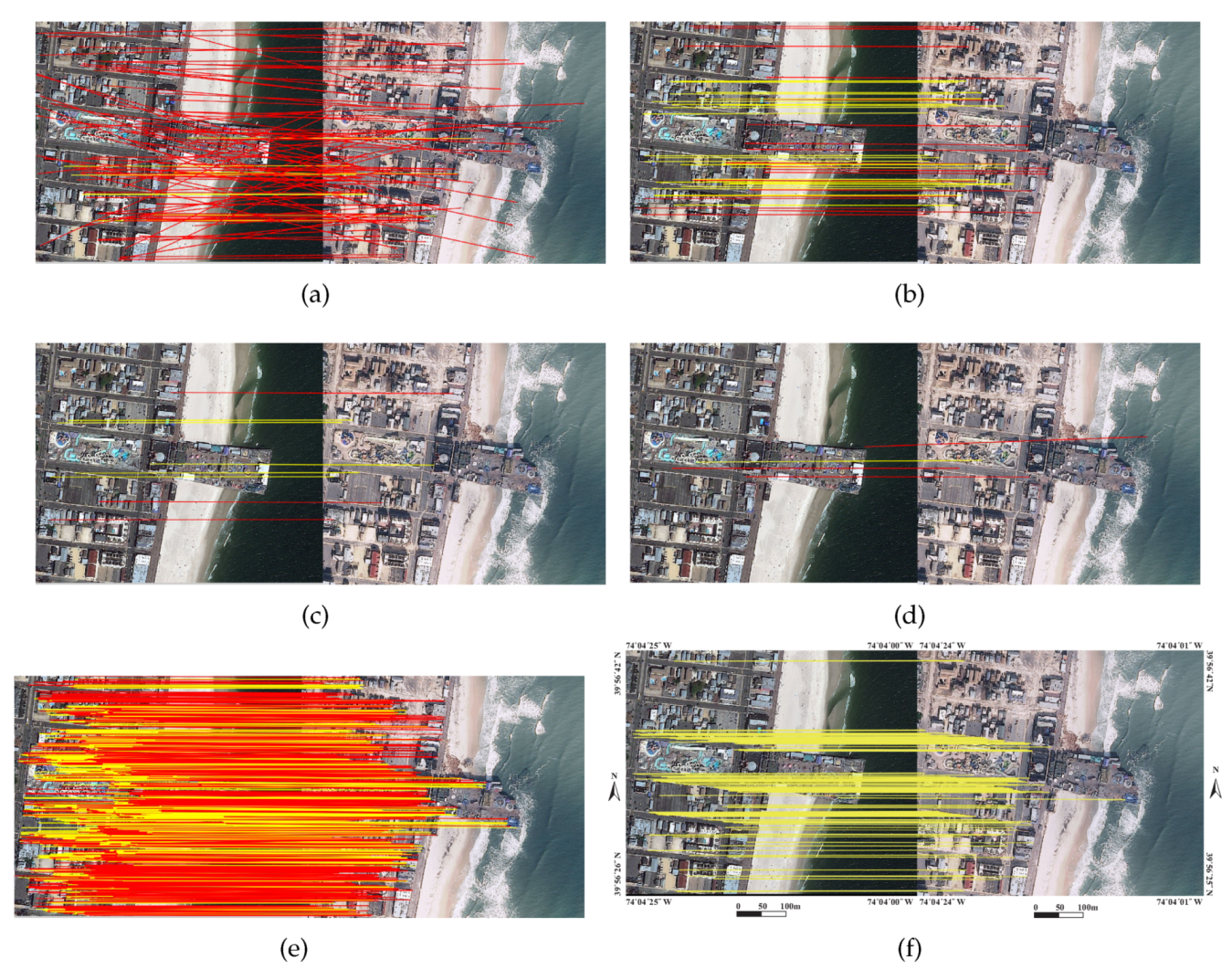
Figure 10 depicts a comparison of matching results for image pair 2. This image pair has many line features, and most buildings are kept intact before and after the hurricane. However, viewpoints change slightly between this image pair, so the tilt and shadow of buildings will considerably impact line feature-based algorithms. The line segments or intersections of the top of buildings are in different positions in the reference and target images because the top of the building is not in the same plane as the ground. Consequently, matching error easily occurs. The false matches of LJL in Figure 10e are mostly at the top of buildings. The proposed algorithm eliminates many false matches at the top of buildings, and the reserved matches are mostly clustered on the ground, thus ensuring registration accuracy.

Figure 11 is the comparison of matching results for image pair 3. Flood seriously damages the farmland and towns located in the lower left of the image. The correct matches of SIFT, LP and MSLD are clustered in the airport area, and the uneven distribution decreases the registration accuracy. LJL has uniform matching distribution and can achieve sub-pixel accuracy registration, but it has many false matches. RLI and the proposed algorithm can achieve 100% $Precision$ on this image pair, indicating that RLI performs better on images with salient features and small variations.

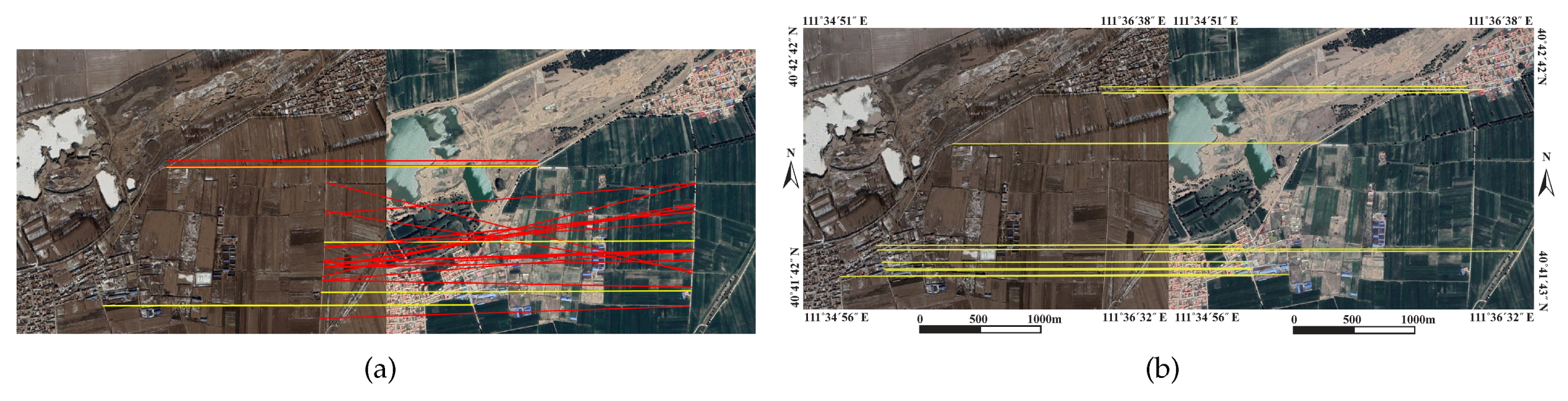
The image pair in Figure 12 is a farmland area that has rich line features. The spectral information between images varies much, and SIFT, LP, MSLD, and RLI fail to register due to changes in geomorphological features caused by seasonal variation. LJL has poor matching results and also fails registration for these images whose line features are not distinct and dense. Meanwhile, the proposed algorithm remains robust.

Figure 13 and Figure 14 depict that the proposed method perform robust on image pairs with scale variation and partial overlap, respectively, whereas LJL has low precision with numerous correct matches. However, the proposed method perform relatively worse on images with large-scale variation. Fewer correct matches result in lower registration accuracy than other experiments. Besides, the intersections in Figure 14 are unevenly distributed due to few artificial objects.

3.5. Comparison and Analysis of Outlier Filtering

To further evaluate the performance of the LIL outlier removal algorithm, we compare it with RANSAC on real remote sensing images for analysis. IN is the number of initial matches, IC is the number of correct matches in the set of initial matches, and IF is the initial number of false matches. The experimental results of LIL outlier removal and RANSAC are listed in

Table 6. Experimental results of RANSAC and LIL outlier removal on real remote sensing images.

	Initial Matches			RANSAC						LIL
	IN	IC	IF	CN	FN	DF	DC	RMSE	Time ${}^{\mathit{a}}$	CN	FN	DF	DC	RMSE	Time
1	105	15	90	10	8	82	7	16.34	0.32	14	0	90	1	0.80	0.35
2	643	263	380	260	110	270	3	2.89	0.08	190	0	380	73	0.60	8.74
3	594	342	252	338	89	163	4	2.32	0.02	320	0	252	22	0.45	6.88
4	167	19	148	18	21	127	1	13.18	0.34	19	0	148	0	0.69	0.89
5	310	24	286	3	17	269	21	—	0.39	20	1	285	4	1.17	2.14
6	142	30	112	28	22	90	2	35.37	0.33	29	1	111	1	0.99	0.62

${}^a$ The time unit is (s).

. The estimated affine models of RANSAC are inaccurate, and the registration errors are large. Compared with LIL outlier removal, RANSAC detects a similar number of correct matches but reserves many false matches. By contrast, LIL can remove nearly all false matches and retain as many correct matches as possible.

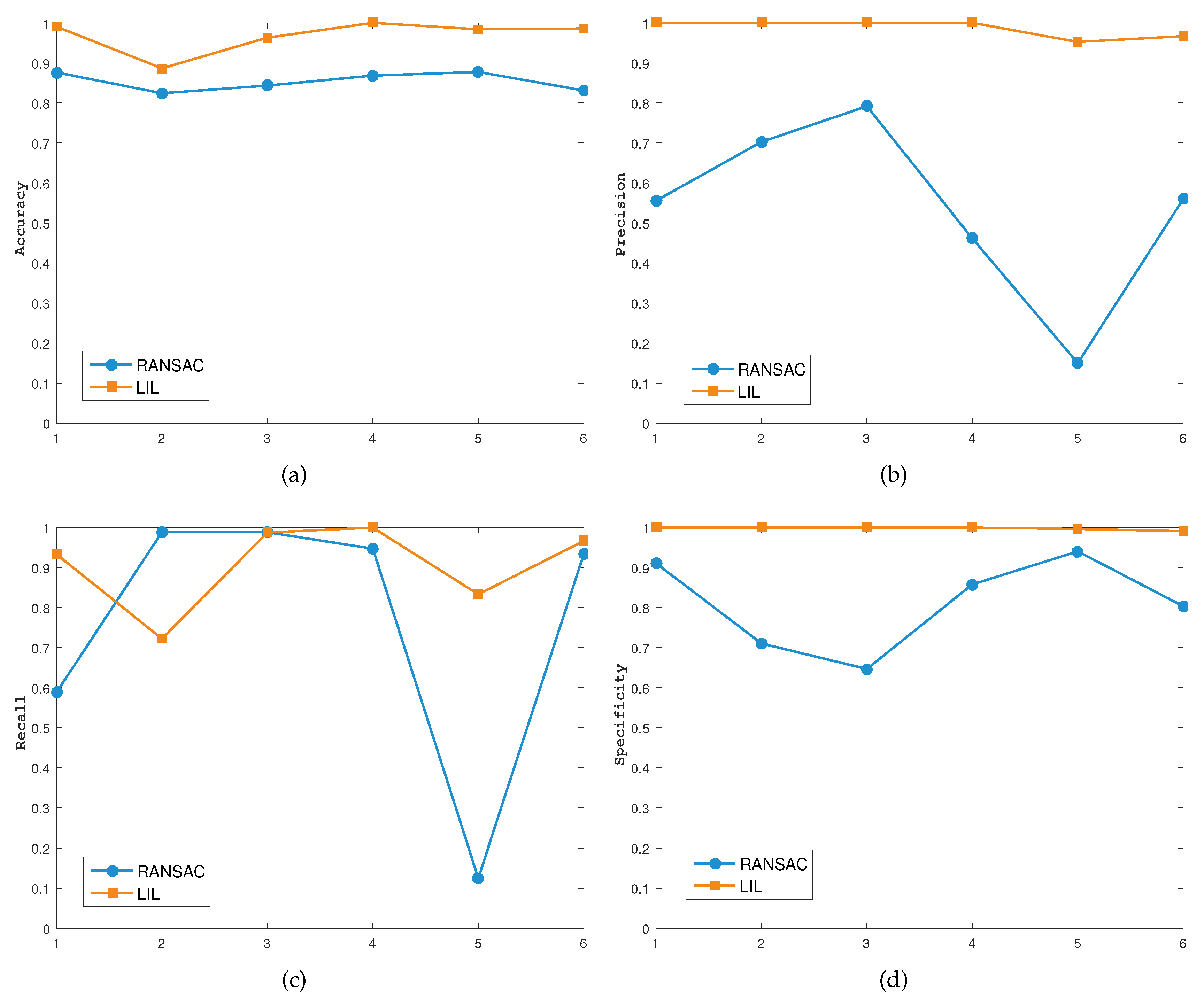
According to Table 6, $Accuracy$, $Precision$, $Recall$, and $Specificity$ can be calculated, as shown in Figure 15. Among the four indicators, the $Accuracy$, $Precision$, and $Specificity$ of LIL are all higher than those of RANSAC, and the detected matches conform to the actual situation more accurately, with a lower false alarm rate. $Recall$ is relatively low, i.e., LIL is weak in identifying correct matches. The reason is that some correct matches with large registration error are eliminated to ensure high registration accuracy. Given that sufficient correct matches are selected, a transformation model with high accuracy can be estimated.

For image pair 2 (which has a low $Recall$ of LIL outlier removal), we analyze the $RMSE$ of correct matches, as shown in

Table 7. RMSE distribution of correct matches detected by RANSAC and LIL outlier removal (image pair 2).

$\mathit{RMSE}$	[0, 1)	[1, 2)	[2, 3)
RANSAC	65	105	90
LIL	65	84	41

. LIL removes numerous matches with relatively high errors, so the estimated transformation model is more accurate than that of RANSAC, and its registration accuracy is higher.

Time consumptions of RANSAC and LIL outlier removal are listed in Table 6. RANSAC takes less time than the proposed method. In terms of image pairs 1, 4, and 6, the computational cost of LIL is closed to that of RANSAC. Because the dimension of variation matrix of relative position is relative to initial matches number, the time complexity is $O(n^2/2)$. Therefore, the computational time of image pairs 2 and 3 is much higher than that of others.

4. Discussion

The proposed LIL-based registration algorithm for satellite remote sensing images performs well on simulated and real images with urban scenes.

On images with simulated transformations, the LIL structure has large scale and rotation invariance. Compared with the algorithms based on line matching, i.e., LP and MSLD, the proposed algorithm’s intersections are more robust to edge fragmentation and occlusion, and the positioning accuracy are higher. The proposed algorithm can resist large scale, rotation, illumination variations, and occlusion conditions, achieving registration with sub-pixel accuracy and high precision on general images. In addition, the matching results show that the LIL local descriptor has higher discriminability compared with the SIFT descriptor.

For real images with large background variations, the average $RMSE$ and $Precision$ of the proposed algorithm are 0.78 and 99.1%, respectively. By contrast, SIFT, LP and MSLD, which use only local gradient information and local structural constraints, have relative low registration accuracy or are even unable to register on images with large global geographic structure variations. The robustness of RLI is poor. RLI selects triplets of intersections of matching lines for registration iteratively. The performance of intersection matching depends on line matching. For images with small variations, high-accuracy registration can be achieved. However, for images with large background variations, if matches used for initial model estimation have large registration error, then the process of iterative refinement for transformation model easily diverges. LJL performs the second best among all methods, verifying the stability of the LJL structure, but the LJL descriptor is weak in resisting large radiation variations, as in image pair 4. In addition, although LJL can detect numerous correct matches, it has high computational complexity and is time consuming for describing and matching. Each LJL constructed in the original images is adjusted to all images in the pyramids and is described there, whereas the proposed algorithm describes each LIL only once. The LJL match propagation also need more calculation steps including local homography estimation and individual line segment matching, whereas the LIL outlier removal only uses simple affine properties and propagates once. For remote sensing images with complex textures, for example, measured on a 2.8 GHz Inter (R) Core (TM) processor with 16 GB of RAM, LJL consumes approximately 2 h to register an image pair with about 5000 and 4000 LJLs, whereas LIL takes around 1 min 10 s, which shows a great reduction in computational cost.

The reasons for the excellent performance of the proposed algorithm are as follows: (1) The LIL structure can well describe the contours of objects in the image, and intersections can reduce the impact of broken line segments and have more accurate positioning, against large background variations; (2) The LIL local feature description utilizes the neighborhood information of two lines and their intersection, and the division of descriptor region is more detailed than that of LBD and RLI. Besides, differing from traditional circular descriptors such as SIFT and LJL, the double-rectangular descriptor contain more structural information; (3) The LIL outlier removal strategy by using LIL structure and relative position changes between any of LILs can eliminate nearly all false matches that do not conform to the spatial relations given many stubborn outliers in the matching set. The proposed algorithm performs well in most remote sensing images of urban areas.

The proposed algorithm still has some limitations. (1) Intersections tend to be unevenly distributed due to the influence of line segment distribution. Clustered in some areas, many similar points with closed positions bring difficulties to the matching process; (2) The division and dimension of the descriptor are not the optimal solution. The width and length of blocks are not adaptive; instead, they depend on empirical values. Moreover, the division of the line support region along the direction of line segment leads to excessive descriptor dimensions and increases computational complexity; (3) The proposed algorithm has many false matches in the initial matching set and relies too much on the LIL outlier removal algorithm. Future work includes optimizing the structure and parameters of the descriptor to retain more significant features.

5. Conclusions

Given that many contours and edges exist in urban areas and the locations of intersections are less affected by large background variations than that of line segments, this paper proposes a registration algorithm based on line-intersection-line structure on satellite remote sensing images with urban scenes. The local information and spatial relations of LIL structure are utilized to design a description and matching strategy. First, multi-scale line segments are detected, and some constraints are implemented to extract LIL features. Next, LIL local descriptors are constructed with the pixel gradients of the LIL neighborhood to realize preliminary matching. Finally, a graph-based LIL outlier removal method is implemented using the LIL structure and variations in the relative position between matches in reference and target images. Outliers are eliminated successively to estimate the affine transformation model.

The proposed algorithm performs well on simulated and real images. It can resist large scale, rotation, illumination, and occlusion variations. It has good robustness against large background variations, achieving sub-pixel accuracy and high precision registration. The LIL local descriptor has discriminability and invariance. In addition, the LIL outlier removal strategy can identify as many false matches as possible and retain sufficient correct matches to estimate a high-accuracy transformation model with high robustness.

In summary, the proposed algorithm is more accurate and robust against background variations compared with the compared state-of-the-art methods. The parameters and structure of LIL will be further optimized in the future.

References

- Lowe, D.G. Distinctive Image Features from Scale-Invariant Keypoints. Int. J. Comput. Vis. 2004, 60, 91–110. [Google Scholar] [CrossRef]
- Bay, H.; Tuytelaars, T.; Van Gool, L. Surf: Speeded up robust features. In European Conference on Computer Vision; Springer: Berlin, Germany, 2006; pp. 404–417. [Google Scholar]
- Ke, Y.; Sukthankar, R. PCA-SIFT: A more distinctive representation for local image descriptors. In Proceedings of the 2004 IEEE Computer Society Conference on Computer Vision and Pattern Recognition, Washington, DC, USA, 27 June–2 July 2004. [Google Scholar]
- Morel, J.M.; Yu, G. ASIFT: A New Framework for Fully Affine Invariant Image Comparison. Siam J. Imaging Sci. 2010, 2, 438–469. [Google Scholar] [CrossRef]
- Sedaghat, A.; Mokhtarzade, M.; Ebadi, H. Uniform Robust Scale-Invariant Feature Matching for Optical Remote Sensing Images. IEEE Trans. Geosci. Remote Sens. 2011, 49, 4516–4527. [Google Scholar] [CrossRef]
- Dellinger, F.; Delon, J.; Gousseau, Y.; Michel, J.; Tupin, F. SAR-SIFT: A SIFT-like algorithm for SAR images. IEEE Trans. Geosci. Remote Sens. 2015, 53, 453–466. [Google Scholar] [CrossRef]
- Fischler, M.A.; Bolles, R.C. Random sample consensus: A paradigm for model fitting with applications to image analysis and automated cartography. Commun. ACM 1981, 24, 381–395. [Google Scholar] [CrossRef]
- Aguilar, W.; Frauel, Y.; Escolano, F.; Martinez-Perez, M.E.; Espinosa-Romero, A.; Lozano, M.A. A robust graph transformation matching for non-rigid registration. Image Vis. Comput. 2009, 27, 897–910. [Google Scholar] [CrossRef]
- Liu, Z.; An, J.; Jing, Y. A simple and robust feature point matching algorithm based on restricted spatial order constraints for aerial image registration. IEEE Trans. Geosci. Remote Sens. 2012, 50, 514–527. [Google Scholar] [CrossRef]
- Zhang, K.; Li, X.Z.; Zhang, J.X. A Robust Point-Matching Algorithm for Remote Sensing Image Registration. IEEE Geosci. Remote Sens. Lett. 2013, 11, 469–473. [Google Scholar] [CrossRef]
- Alajlan, N.; El Rube, I.; Kamel, M.S.; Freeman, G. Shape retrieval using triangle-area representation and dynamic space warping. Pattern Recognit. 2007, 40, 1911–1920. [Google Scholar] [CrossRef]
- Shi, X.; Jiang, J. Point-matching method for remote sensing images with background variation. J. Appl. Remote Sens. 2015, 9, 095046. [Google Scholar] [CrossRef]
- Zhao, M.; An, B.; Wu, Y.; Luong, H.V.; Kaup, A. RFVTM: A Recovery and Filtering Vertex Trichotomy Matching for Remote Sensing Image Registration. IEEE Trans. Geosci. Remote Sens. 2017, 55, 375–391. [Google Scholar] [CrossRef]
- Von Gioi, R.G.; Jakubowicz, J.; Morel, J.M.; Randall, G. LSD: A fast line segment detector with a false detection control. IEEE Trans. Pattern Anal. Mach. Intell. 2010, 32, 722–732. [Google Scholar] [CrossRef] [PubMed]
- Akinlar, C.; Topal, C. EDLines: A real-time line segment detector with a false detection control. Pattern Recognit. Lett. 2011, 32, 1633–1642. [Google Scholar] [CrossRef]
- Wang, Z.; Wu, F.; Hu, Z. MSLD: A robust descriptor for line matching. Pattern Recognit. 2009, 42, 941–953. [Google Scholar] [CrossRef]
- Zhang, L.; Koch, R. An efficient and robust line segment matching approach based on LBD descriptor and pairwise geometric consistency. J. Vis. Commun. Image Represent. 2013, 24, 794–805. [Google Scholar] [CrossRef]
- Shi, X.; Jiang, J. Automatic Registration Method for Optical Remote Sensing Images with Large Background Variations Using Line Segments. Remote Sens. 2016, 8, 426. [Google Scholar] [CrossRef]
- Yammine, G.; Wige, E.; Simmet, F.; Niederkorn, D.; Kaup, A. Novel similarity-invariant line descriptor and matching algorithm for global motion estimation. IEEE Trans. Circuits Syst. Video Technol. 2014, 24, 1323–1335. [Google Scholar] [CrossRef]
- Long, T.; Jiao, W.; He, G.; Wang, W. Automatic line segment registration using Gaussian mixture model and expectation-maximization algorithm. IEEE J. Sel. Top. Appl. Earth Obs. Remote Sens. 2014, 7, 1688–1699. [Google Scholar] [CrossRef]
- Zhao, C.; Zhao, H.; Lv, J.; Sun, S.; Li, B. Multimodal image matching based on multimodality robust line segment descriptor. Neurocomputing 2016, 177, 290–303. [Google Scholar] [CrossRef]
- Jiang, J.; Cao, S.; Zhang, G.; Yuan, Y. Shape registration for remote-sensing images with background variation. Int. J. Remote Sens. 2013, 34, 5265–5281. [Google Scholar] [CrossRef]
- Yavari, S.; Zoej, M.J.V.; Salehi, B. An automatic optimum number of well-distributed ground control lines selection procedure based on genetic algorithm. ISPRS J. Photogramm. Remote Sens. 2018, 139, 46–56. [Google Scholar] [CrossRef]
- Fan, B.; Wu, F.; Hu, Z. Line matching leveraged by point correspondences. In Proceedings of the 2010 IEEE Computer Society Conference on Computer Vision and Pattern Recognition, San Francisco, CA, USA, 13–18 June 2010; pp. 390–397. [Google Scholar]
- Zhao, M.; Wu, Y.; Pan, S.; Zhou, F.; An, B.; Kaup, A. Automatic Registration of Images With Inconsistent Content Through Line-Support Region Segmentation and Geometrical Outlier Removal. IEEE Trans. Image Process. 2018, 27, 2731–2746. [Google Scholar] [CrossRef] [PubMed]
- Sui, H.; Xu, C.; Liu, J.; Hua, F. Automatic optical-to-SAR image registration by iterative line extraction and Voronoi integrated spectral point matching. IEEE Trans. Geosci. Remote Sens. 2015, 53, 6058–6072. [Google Scholar] [CrossRef]
- Li, K.; Yao, J.; Lu, X.; Li, L.; Zhang, Z. Hierarchical line matching based on Line-Junction-Line structure descriptor and local homography estimation. Neurocomputing 2016, 184, 207–220. [Google Scholar] [CrossRef]
- Lyu, C.; Jiang, J. Remote sensing image registration with line segments and their intersections. Remote Sens. 2017, 9, 439. [Google Scholar]
- Han, X.; Leung, T.; Jia, Y.; Sukthankar, R.; Berg, A.C. Matchnet: Unifying feature and metric learning for patch-based matching. In Proceedings of the IEEE Conference on Computer Vision and Pattern Recognition, Boston, MA, USA, 7–12 June 2015; pp. 3279–3286. [Google Scholar]
- Kanazawa, A.; Jacobs, D.W.; Chandraker, M. Warpnet: Weakly supervised matching for single-view reconstruction. In Proceedings of the IEEE Conference on Computer Vision and Pattern Recognition, Las Vegas, NV, USA, 27–30 June 2016; pp. 3253–3261. [Google Scholar]
- Rocco, I.; Arandjelovic, R.; Sivic, J. Convolutional neural network architecture for geometric matching. In Proceedings of the IEEE Conference on Computer Vision and Pattern Recognition, Honolulu, HI, USA, 21–26 July 2017; Volume 2. [Google Scholar]
- He, H.; Chen, M.; Chen, T.; Li, D. Matching of Remote Sensing Images with Complex Background Variations via Siamese Convolutional Neural Network. Remote Sens. 2018, 10, 355. [Google Scholar] [CrossRef]
- Yang, Z.; Dan, T.; Yang, Y. Multi-temporal Remote Sensing Image Registration Using Deep Convolutional Features. IEEE Access 2018, 6, 38544–38555. [Google Scholar] [CrossRef]
- Leordeanu, M.; Hebert, M. A Spectral Technique for Correspondence Problems Using Pairwise Constraints. In Proceedings of the Tenth IEEE International Conference on Computer Vision (ICCV’05), Beijing, China, 17–21 October 2005; pp. 1482–1489. [Google Scholar]
Figure 1.
Flowchart of the LIL algorithm.
Figure 2.
Multi-scale Gaussian pyramid.
Figure 3.
Diagram of the LIL structure.