Towards a Unified and Coherent Land Surface Temperature Earth System Data Record from Geostationary Satellites

Abstract

Our objective is to develop a framework for deriving long term, consistent Land Surface Temperatures (LSTs) from Geostationary (GEO) satellites that is able to account for satellite sensor updates. Specifically, we use the Radiative Transfer for TOVS (RTTOV) model driven with Modern-Era Retrospective Analysis for Research and Applications (MERRA-2) information and Combined ASTER and MODIS Emissivity over Land (CAMEL) products. We discuss the results from our comparison of the Geostationary Operational Environmental Satellite East (GOES-E) with the MODIS Land Surface Temperature and Emissivity (MOD11) products, as well as several independent sources of ground observations, for daytime and nighttime independently. Based on a six-year record at instantaneous time scale (2004–2009), most LST estimates are within one std from the mean observed value and the bias is under 1% of the mean. It was also shown that at several ground sites, the diurnal cycle of LST, as averaged over six years, is consistent with a similar record generated from satellite observations. Since the evaluation of the GOES-E LST estimates occurred at every hour, day and night, the data are well suited to address outstanding issues related to the temporal variability of LST, specifically, the diurnal cycle and the amplitude of the diurnal cycle, which are not well represented in LST retrievals form Low Earth Orbit (LEO) satellites.

1. Introduction

Land surface temperature is an important climate parameter due to its control of the components of the surface energy budget, such as turbulent heat and moisture fluxes, and upward terrestrial radiation [1]. For climate applications, information is needed on large scales, and ideally, the diurnal cycle needs to be resolved. In this study, we develop an approach to derive information on LST which is applicable to the GOES satellites across multiple missions and multiple satellite sensors. We report on results obtained during the period (2004–2009) at hourly time intervals, at about 5-km spatial resolution.

Since surface ground observations are limited, shelter temperature has been widely used as a proxy to surface skin temperature to meet large-scale needs. Issues emerging from such an approach have been addressed previously [2]. While observations from satellites are considered useful for inferring LST, only a few satellite sensors observe all the necessary parameters needed to derive LST with high accuracy. Some lack sufficient number of channels to account simultaneously for atmospheric effects (as needed for implementing the “split window” approach) [3,4,5,6,7]. Others do not observe the Earth surface at high frequency to resolve the diurnal cycle, or at high spatial resolution, to minimize the presence of clouds.

Information on surface emissivity is also not readily available at sufficient spectral resolution [8,9]. Moreover, land surface emissivity is generally less than one, and therefore, part of the atmospheric downward radiation is reflected by the surface and has to be accounted for [10] when converting ground observations of radiative flux measurements to LST (which is not always done). The number of successful attempts to derive LST from satellites has been substantial (especially using the well-established split window approach). A full review of what was done is beyond the scope of this paper, but a comprehensive summary can be found in Li et al. [11], and is briefly presented below.

The early effort to retrieve LST from satellites over agricultural land made by Price [3] was done by adopting the Advanced Very High Resolution Radiometer (AVHRR) Sea Surface Temperature (SST) split window algorithm [12,13]. Becker and Li [14] extended the split window method of McMillin [15] for SST to LST and took into account the spectral variability in land surface emissivity. This so called “generalized split window” LST algorithm has been widely used. Additional efforts include the work of Prata, [16], Sobrino et al. [7], Wan and Dozier [5], Francois and Ottle [17], Coll and Caselles [18], Trigo et al. [19], and Wan [20]. The approach for accounting for emissivity has evolved from assignments based on land use to the use of the Normalized Difference Vegetation Index (NDVI) [21,22,23]; however, the NDVI concept is not applicable for every surface type. Currently, surface emissivity is derived from the Advanced Space Thermal Emission and Reflection Radiometer (ASTER), the Thermal Infrared (TIR) Multispectral Scanner (TIMS), and the Moderate-resolution Imaging Spectroradiometer (MODIS) [24,25,26,27,28,29] culminating in the Combined ASTER and MODIS Emissivity over Land (CAMEL) product to be used here [30,31].

Most of the above referenced studies focus on polar orbiting satellites such as the National Oceanic and Atmospheric Administration (NOAA)-AVHRR, the Along-Track Scanning Radiometer (ATSR) and the MODIS instrument aboard Terra and Aqua satellites; the temporal measurement frequency of these satellites is approximately twice per day. The Land Surface Diurnal Temperature Range (DTR) is an important element of the climate system and is not captured by the polar orbiting satellites. Geostationary satellites provide diurnal coverage and observe the surface continuously at a nadir pixel resolution of about 4 km [32] which led to the development of several algorithms for GEO satellites [33,34,35].

While the principles of retrieval methodologies have not changed drastically over time, the development in auxiliary information, quality of such information, and availability of long term records of satellite observations make it feasible to formulate a homogeneous approach across various satellite sensors that can culminate in climatic records of LST. The primary objective of this study is to present a methodology that can be implemented with different GOES observing systems, using consistent auxiliary information of highest possible quality and utilizing radiative transfer models that account for the vertical profiles of atmospheric states for each retrieval. From mid-2004 to 2017, only one thermal channel is available on the GOES series; the focus of this study is on retrievals using such a single channel in order that a consistent, long term record can be generated from all the GOES satellites (including those that allow the implementation of the split window approach). In Section 2, materials used are described; retrieval algorithm development is presented in Section 3; evaluation of GOES-E based LST estimates is presented in Section 4; a discussion is provided in Section 5; and a summary is presented in Section 6.

2. Materials

2.1. GOES Satellite Data

The GOES system is operated by the National Oceanic and Atmospheric Administration, National Environmental Satellite, Data and Information Service (NESDIS). The GOES system is based on the use of satellites designed to operate at an orbit of 35,790 km above the earth, remaining stationary to a given point on the ground. The GOES provides data at high temporal frequency (15 min) with continental-scale coverage (N. and S. America). In this study observations from GOES-12 (4/1/2003–4/14/2010) will be utilized (

Table 1. Summary of GOES-8/GOES-12 channels.

Satellite	Channel	Symbol	Wavelength	Objective	Spatial Resolution (Nadir)
GOES-8 & GOES12	1	R1	0.67 μm	Cloud	1 km × 1 km
	2	R2 and T2	3.9 μm	Cloud and snow	4 km × 4 km
	3	T3	6.7 μm	Water vapor	4 km × 4 km
	4	T4	10.7 μm	Surface temperature	4 km × 4 km
GOES-8	5	T5	12.0 μm	Sea surface temperature and water vapor	4 km × 4 km
GOES12	6	T6	13.3 μm	……	4 km × 4 km

Note: GOES-8 information is provided since cloud algorithm was originally developed for GOES-8. Channel 2 is separated into the reflected solar radiation component (R2) and the emitted infrared radiation component (T2) [52]; Channel 3 is not used in any of the cloud screening tests.

). Typically, the GOES imager includes five spectral channels (one visible, four infrared). For GOES 8-10 the channels are located at 3.9, 6.75, 10.7, and 12.2 µm whereas for GOES 11–15, the 6.75 µm channel was moved to 6.5 µm and the 12 µm channel was moved to 13.3 µm. The visible, mid-infrared and 11 µm band are typically used for cloud screening while the two thermal infra-red (TIR) bands (10.2–11.2 µm and 11.5–12.5 µm) are used in what is known as a “split-window” approach to retrieve LST.

Aspects of GOES satellite systems that need to be addressed before deriving LST include the spectral characteristics of the GOES sensors and their filter functions, calibration of visible and IR channels, cloud screening methodology (that requires snow analysis information) and the selection of cloud screening tests as appropriate for each satellite configuration, with special distinction between night-time and day-time conditions. Over the period of this study, two separate operational GOES Imagers, one located at a longitude of −75° (referred to as GOES-East) and one located at a longitude of −135° (referred to as GOES-West) continuously provided imagery over North and South America. In this study, observation from GOES-East only will be utilized for years 2004–2009. The temporal sampling of the GOES Imager is every 30-min over North America and every 3-h over the full disk. Spectral distribution of the GOES 8–15 series are provided in NOAA NESDIS STAR GOES Imager LST ATBD (Version 3.0).

2.2. Visible and Thermal Channel Calibration

Visible channels are used in the cloud screening part of data processing. Their calibration is done in two stages. First, applied are the pre-launch calibration coefficients to get the first step “nominal reflectance” (Apre), and then, the post-lunch calibration coefficients are applied to obtain the final calibrated nominal reflectance (Apost).

The nominal reflectance is defined as the ratio of reflected radiance to nominal solar irradiance given as:

Apre = pi*R/F₀

(1)

where pi = 3.141593, R is satellite observed upwelling radiance, and F₀ is the solar irradiance at local zenith and mean Sun-Earth distance.

The pre-launch nominal reflectance is:

Apre = k (X − Xspace)

(2)

where k is the pre-launch calibration constant to convert satellite observed digital counts to nominal reflectance. X is the instrument raw digital count, Xspace is the raw count of the space scene (has been adjusted to 29 for all GOES imagers at NOAA). The Post-lunch calibration is applied by multiplying the Apre by a coefficient:

Apost = Apre*C

(3)

The pre-launch coefficient for GOES-12 for radiance calibration was 0.5771 and for nominal reflectance it was 0.001141.

NOAA/STAR monitors the GOES imager and updates the post-launch coefficients every month. Coefficients are considered optimal for the days on or after the second Tuesday of the month following the coefficient generation month. For more details, see: http://www.star.nesdis.noaa.gov/smcd/spb/fwu/homepage/GOES_Imager_Vis_OpCal.php.

Inter-calibration of the infrared channels on the GOES series of satellites has been performed using under-passes of the well calibrated NASA Atmospheric Infrared Sounder (AIRS) sensor on the Aqua platform [36]. Infrared imager data from GOES are stored in GOES Variable Format (GVAR) counts and radiances can be derived from GVAR counts by applying the calibration and scaling coefficients using a procedure described in [37].

Calibration of IR channels of GOES imager data is also done in two stages: (1) converting the imager GVAR raw count to scene radiance; (2) converting the radiance to temperature. To convert a 10-bit GVAR count to scene radiance we use:

R = (X − b)/m

(4)

where X is the GVAR raw count (10-bit, range from 0 to 1023), m and b are calibration coefficients. The values for m and b depend on channel selected, but are constant for a given channel. The obtained radiance can be convert to effective temperature (K) by inverse of the Planck function:

T_eff = C₂*n/ln (1 + C₁*n³/R)

(5)

C₁ = 1.191066 × 10e⁻⁵ [m·W/(m²·sr·cm⁻⁴)], C₂ = 1.438833 (K/cm⁻¹), “n” is the central wave-number of the channel and varies from instrument to instrument.

The effective temperature T_eff is further converted to actual temperature by:

T = a + b *T_eff + g* T_eff²

(6)

where “a”, “b” and “g” are coefficients and their values and central wave-numbers can be found at: https://www.ospo.noaa.gov/Operations/GOES/calibration/gvar-conversion.html#radiance.

Evaluation of calibration was done by comparison of radiances in each channel with NOAA values.

2.3. Emissivity Data

A new land surface emissivity Earth Science Data Systems (ESDS) product has been developed in support of a NASA Making Earth System Data Records for Use in Research Environments (MEaSUREs) project [30,31] MODIS-ASTER Global Infrared Combined Emissivity product produced from the University Wisconsin Global Infrared Land Surface Emissivity (UWIREMIS) and the ASTER Global Emissivity (GED) Database are known as the Combined ASTER and MODIS Emissivity for Land (CAMEL) and represents a combination of MODIS baseline-fit emissivity database (MODBF). The CAMEL ESDR is produced globally at 5-km resolution at mean monthly time-steps and for 13 bands from 3.6–14.3 micron and extended to 417 bands using a Principal Component (PC) regression approach. This product has been used in our retrievals of LST.

2.4. MERRA-2 Data

The 6 hourly MERRA-2 re-analysis data (MERRA-2 inst6_3d_ana_Np version 5.12.4) (https://disc.gsfc.nasa.gov/datasets/M2I6NPANA_V5.12.4/summary) are used to specify the atmospheric conditions [38]. The re-analysis data are available at [00, 06, 12, 18] hours with a resolution of 0.5° × 0.625°, for 42 pressure levels. Properties include sea-level pressure, surface pressure, geopotential height, air temperature, wind components, and specific humidity. Since the LST is retrieved at hourly time scale, the MERRA-2 data are linearly interpolated in time to give the atmospheric state in between the four analysis times (as needed for input to RTTOV) and linearly interpolated to 0.05° × 0.05° in space to match the formulation of this study.

2.5. MOD11

The GOES based LST estimates will be evaluated against LST retrievals from MOD11 Version 6 Land Surface Temperature and Emissivity product [20] (we use both MOD11_L2 data and MOD11C3 data). The MODIS LST data products are produced as a series of nine products. The sequence begins as a swath at a nominal pixel spatial resolution of 1 km at nadir and a nominal swath coverage of 2030 or 2040 lines along track by 1354 pixels per line in the daily LST product [39]. There are two algorithms used in the daily MODIS LST processing: the generalized split-window LST algorithm [5] and the day/night LST algorithm. New refinements made to these two algorithms are described by Wan [20]. The MOD11_L2 version 6 swath product provides per-pixel land surface temperature (LST) and emissivity. It is produced daily in 5-min temporal increments of satellite acquisition and has a pixel size of 1 km. The MOD11C3 Version 6 product provides monthly land surface temperature (LST) and emissivity values in a 0.05 (5600 m × 5600 m) degree latitude/longitude climate modeling grid (CMG), which has a Geographic grid with 7200 columns and 3600 rows representing the entire globe. The MOD11C3 granule consists of day and night LST and their corresponding quality indicator (QC) layers.

2.6. Ground Observations

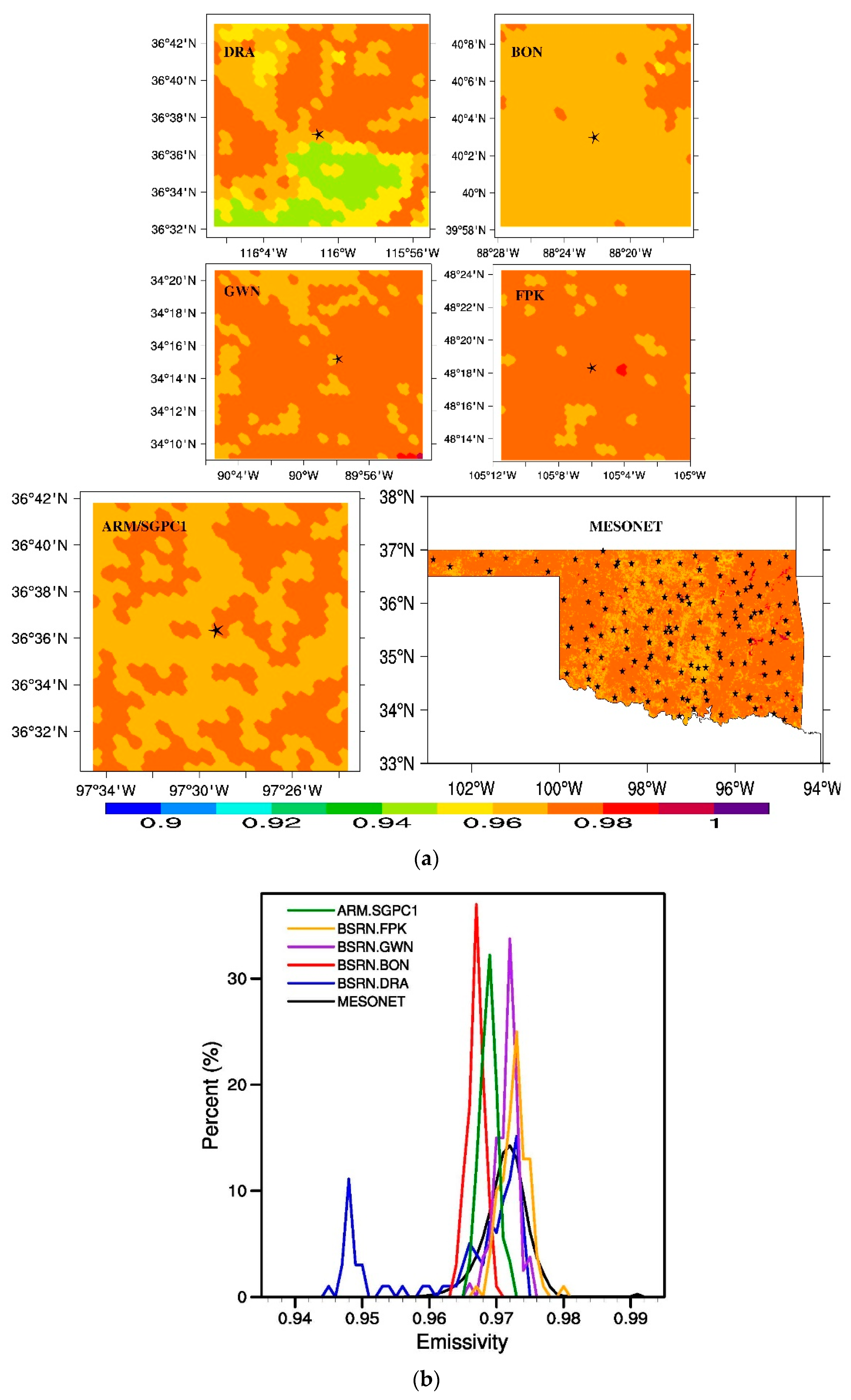
• SURFRAD/BSRN

NOAA established the Surface Radiation Budget Network (SURFRAD) in 1993 [40] to support climate research by providing accurate, continuous, long-term measurements of the surface radiation budget over the United States. These became the continental U.S. contingent of the International Baseline Surface Radiation Network (BSRN) [41] as described in [42]. The SURFRAD Network uses Eppley Precision Infrared Pyrgeometers (model PIR). The general information about the instrumentation can be found at: https://www.esrl.noaa.gov/gmd/grad/surfrad/overview.html.

Specifically, we used the following sites: Desert Rock, Nevada (DRA: 36.62°N, 116.02°W; 1007 m); Fort Peck, Montana (FPK: 48.32°N, 105.10°W; 634 m); Bondville, Illinois (BON: 40.06°N, 88.37°W; 230 m) and Goodwin Creek, Mississippi (GCM: 34.25°N, 89.87°W; 98 m). BSRN sites that provide data at 1 or 3-min frequency, which makes them suitable for generating information to match the satellite observations. The upwelling and downwelling longwave radiative fluxes are measured with a precision infrared radiometer, which is sensitive in the spectral range from 3000 to 50,000 nm.

• ARM SGP

The Atmospheric Radiation Measurement Program (ARM) Near-Surface Observation Dataset came from the ARM Cloud and Radiation Test Bed site (34°–39°N and 94.5°–100.5°W). The average elevation is 314 m. The surface skin temperature used in this paper is observed at 60-sec intervals at the Central Facility (36.6°N, 97.48°W) of the Southern Great Plains (SGP) site. The instrument used to observe the skin temperature is the Infrared Thermometer (IRT). It is a ground-based radiation pyrometer that measures the equivalent blackbody brightness temperature of the scene in its field of view. The downwelling version has a narrow field of view for measuring sky temperature and detecting clouds. The upwelling version has a wide field of view for measuring the narrowband radiating temperature of the ground surface (https://www.arm.gov/capabilities/instruments/irt). Time series and scatter plots are produced and inspected to compare surface temperature measured by the IRT and a precision infrared radiometer (PIR). The temperature measuring range is from 173 to 473 K. The accuracy is the greater value of a) ±0.5 K + 0.7% of the temperature difference between the internal reference temperature and the object measured or b) the temperature resolution. The spectral sensitivity is from 9.6 to 11.5 µm [43].

• Oklahoma MESONET

The Oklahoma MESONET is an automated network of over 110 remote, meteorological stations across Oklahoma (http://www.mesonet.org). The surface types are predominantly grassland/wooded, grassland/cropland. In 1999, infrared temperature (IRT) sensors (Apogee Instruments, Inc.) were installed at 89 of the MESONET sites. A combination of automated and manual tests was applied using simultaneous soil and atmospheric measurements to inter-compare observations and ensure that the skin temperature observations are of research quality [44]. The measurements collected by the MESONET provided a unique opportunity to inter-compare observations. Fiebrich et al. [45] provide an evaluation of 5-min-resolution field measurements collected using the sensors. This sensor was chosen for use because it is water resistant and was designed for continuous outdoor use. Sensor accuracy is approximately ± 0.2 °C from 15 °C to 35 °C and 0.3 °C from 35 °C to 45 °C. The sensor is installed at a height of 1.5 m and has a field of view of a diameter circle of 0.5 m. The energy detected by the sensor is converted to a temperature using the Stefan–Boltzmann law and an assumed surface emissivity of 1.0. Slight underestimation is caused because the true emissivity of the land surface is less than 1.0. In addition, slight overestimation is caused by reflected longwave radiation from the target [46]. While surface reflection of downwelling longwave radiation is ignored, Sun et al. [32] discussed the effects of these two factors and found that the total effect may be a slight underestimation of the skin temperature. Generally, estimated impact of uncertainty in relevant parameters on in situ LST are as follows: radiometric calibration uncertainty of ±0.2 to 0.5 K can impact LST as much as 0.2 K; emissivity uncertainty of ±1% can impact LST by as much as 0.3 K; downwelling atmospheric radiance uncertainty of ±10% can impact LST by as much as 0.1 K [47].

2.7. Cloud Detection

For cloud masking, various ancillary data are needed such as surface type, snow-free channel-1 radiance, and a pixel position information, all in the same dimension and location as the satellite images. The land cover data used in this study for cloud screening implementation, are generated at 1-km resolution [48]. This product includes 14 International Geosphere–Biosphere Programme (IGBP) classes and the underlying surface types are aggregated according to the IGBP classification.

A Coupled Cloud and Snow Detection Algorithm (CCSDA) that was developed initially for use with GOES-8 satellite is adjusted as appropriate for each GOES satellite is used. The algorithm is described in [49,50]. Variants of the approach were tested and evaluated in several publications [51]. In the case of the GOES-8 imager four channels were used to detect clouds, snow, and to perform background analysis for each hour of the diurnal cycle. Beginning with GOES-12, Channel 5 is no longer available (Table 1) [52].

The CCSDA algorithm is capable of producing its own snow analysis using an algorithm that applies three tests using three GOES channels. Alternatively, there is a switch to allow the use of a snow analysis from a different source. The advantage of using the snow analysis generated by the CCSDA algorithm is that it is updated hourly, which provides a more accurate analysis of the expected background when applying the cloud tests. If a daily snow analysis is used, the snow conditions cannot change for each hour of the cloud analysis, and this may introduce error.

In

Table 2. Cloud Screening Tests for GOES-8.

Test	Apply	Cloud Detection Variable	Cloud That May Be Detected
RGCT	Day	R1	Highly-reflective cloud
TGCT	Day and Night	T4	Cold cloud
C2AT	Day	R2	Weakly Reflective Cloud
TMFT	Day and Night	T2 − T4	Water cloud + Cirrus + Other Clouds
FMFT	Day and Night	T4 − T5	Thin Cirrus
ULST	Night	T2 − T4	Nighttime uniform low stratus
CIRT	Night	(T2 − T4)/T4	Nighttime cirrus

Note: Reflectance Gross Contrast Test (RGCT); Channel-2 Albedo Test (C2AT); Thermal Gross Cloud Test (TGCT); Three Minus Five Test (TMFT); Four minus Five Test (FMFT); Uniform Low Stratus Test (ULST); Cirrus IR Test (CIRT).

we present a description of the cloud screening tests used for GOES-8, along with an explanation of how the tests are assembled to determine a clear probability.

The ultimate clear probability (P) can be assembled in various ways on the basis of individual test results. In this method:

$$P=\sqrt[n]{{\displaystyle \prod }_1^n{P}_i}$$

(7)

P_i is the clear probability from each individual cloud screening test and n is the total number of cloud screening tests. This assembly method guarantees that the target pixel is cloudy (P = 0) if any individual test identifies it as cloudy (P_i = 0). Otherwise, it compiles the confidence levels from all of the individual tests to obtain an overall clear probability.

Referring to Table 2, there was only one cloud screening test that required Channel 5, namely, the FMFT test. In the cloud screening algorithm for GOES-12 and beyond, the FMFT test will not be used, and the test assembly method described for GOES-8 is implemented with one less cloud test.

For each cloud test, threshold levels are used to differentiate between clear and cloudy pixels. For each new satellite, it is necessary to test the thresholds and modify as needed. Here, the cloud mask method applies two spatial tests and one threshold test on an 11–3.7 µm difference image. This fourth test compares the temperature from the 11 µm channel to a 20-day clear-sky composite of 11 µm temperatures, and labels the pixel as cloudy if the difference is greater than the threshold. The pixel level data were gridded to 0.05° and compared to the Pathfinder Atmospheres—Extended (PA TMOS-X) product [34]. Agreement above 95% for various times of the day was found. The only region which showed slight disagreement between the two independent cloud masks is over areas of complex terrain in the Western US, but even over these regions the two cloud masks agreed over 85% of the time.

The major difference between the day time and night time algorithms (Table 2) is that there are no Reflectance Gross Contrast Test (RGCT, when visible channel is missing) and Channel-2 Albedo Test (C2AT) during the night time. This will mostly affect the detection of reflective clouds. For GOES-12, the FMFT test could not be used. We have tested the cloud screening algorithm for use at nighttime. We applied the nighttime algorithm on daytime data and compared to results when the full daytime algorithm is used. Evaluation of LST estimates in each case is presented in Figure 1. As this figure shows, the daytime algorithm provides better agreement with ground observations than the nighttime one yet, the differences are small as illustrated in Figure 1.

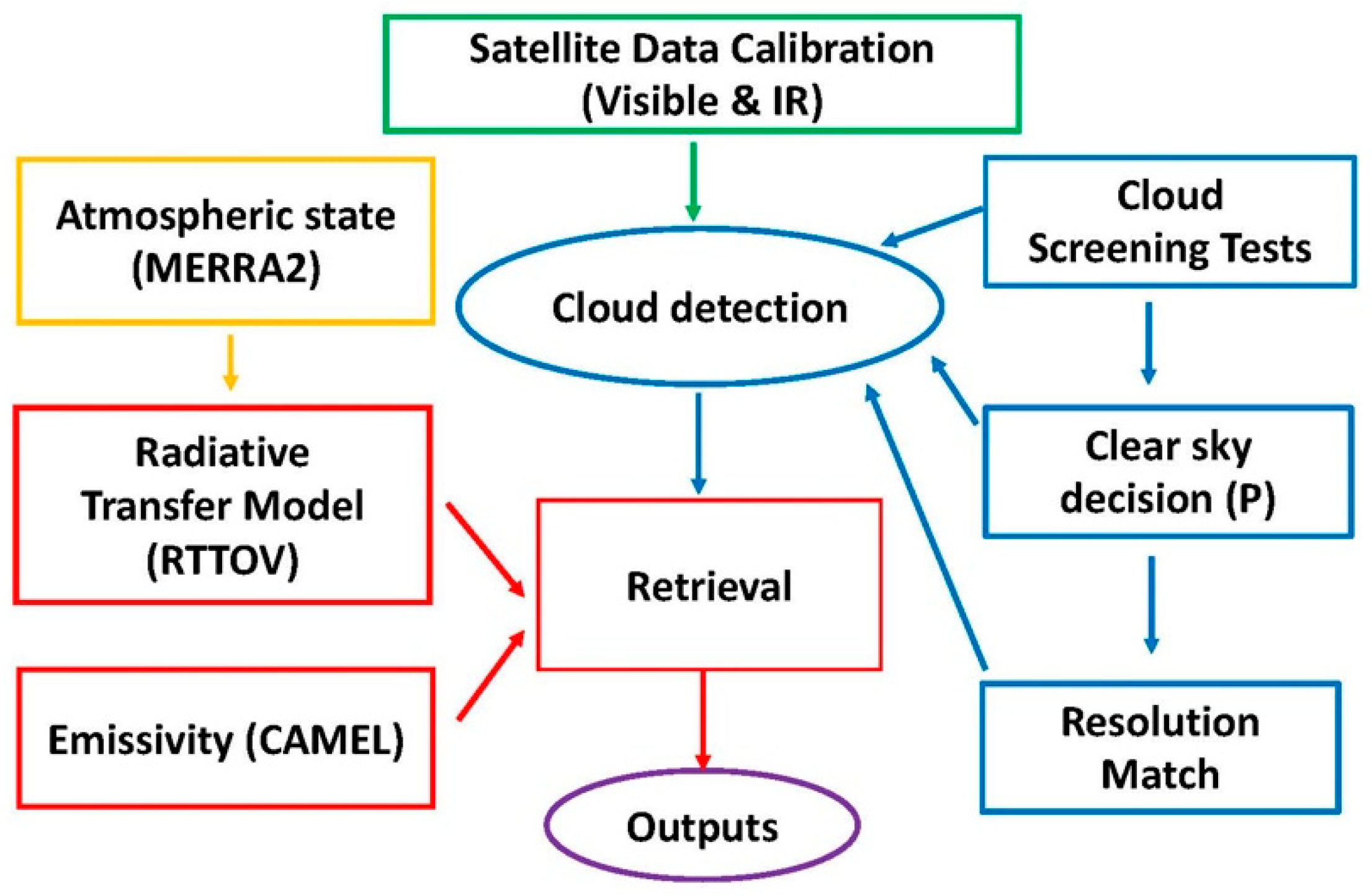
3. LST Retrieval Algorithm Development for GOES Satellites

Satellite observed radiance $R_o^{\uparrow }$, can be expressed as

$$R_o^{\uparrow }=ϵB\left(T_s\right)\mathrm{X}+R_a^{\uparrow }+\left(1-ϵ\right)R_a^{\downarrow }X$$

(8)

where $ϵ$ is surface emissivity, $B\left(T_s\right)$ is blackbody emission at surface temperature $T_s$, $X$ denotes the atmospheric transmittance, $R_a^{\uparrow }$ and $R_a^{\downarrow }$ are atmospheric emission to space and surface, respectively. With known surface emissivity and simulated atmospheric emission and transmittance, the surface temperature can be retrieved

$$T_s=B^{-1}\left[\frac{1}{ϵ}\left(\frac{1}{X}\left(R_o^{\uparrow }-R_a^{\uparrow }\right)-\left(1-ϵ\right)R_a^{\downarrow }\right)\right]$$

(9)

where $B^{-1}$ denote the inverse of Planck function for GOES-12 channel 4.

Here, the approach is based on the Radiative Transfer for TOVS (RTTOV) model v11.2 [53,54,55] adjusted for the GEO characteristics and driven with MERRA-2 reanalysis fields. The CAMEL data are also implemented in the method. The advantage of this approach is that it is consistent with the retrieval approach used at JPL to generate the MOD21 product [56]. The processing sequence is described in Figure 2.

Data processing sequence starts from raw digital counts from GOES satellites. Calibration is applied to all channels. Channel 4 (10.2 to 11.2 um) was used for LST retrieval. All channels except channel 3 (6.7 um) were used in the cloud detection algorithm. After cloud screening, GOES observations were resampled to a uniform grid of 0.05° resolution. The atmospheric radiation and transmittance were simulated with the RTTOV model using MERRA-2 fields as input. The MERRA-2 fields were first temporally interpolated to satellite observation time and then collocated to satellite locations. RTTOV calculated upwelling, downwelling radiances and atmospheric transmittance combined with CAMEL surface emissivity to retrieve the LST according to Equation (11).

4. Evaluation of GOES-E Based LST Estimates

We will present results of evaluation for UMD LST retrievals against MOD11 products, the BSRN/SURFRAD network over the USA, the ARM/SGP C1 site over the Southern Great Plains, and the MESONET network over Oklahoma. The issue of evaluation of satellite products of LST against ground measurements is complex, primarily, due to scale issues and known large spatial variability of LST. A comprehensive discussion on all aspects of validation issues are described by Guillevic et al. [43] and Göttsche et al. [57].

4.1. Scale Issues Related to Satellite and Ground Observations

The ground observations are point observations while the satellite LST product is at pixel level gridded to 0.05°. To assess the homogeneity of each site, we use the ASTER Global Emissivity Dataset at 1-km V003 (DOI: 10.5067/Community/ASTER_GED/AG1km.003) available for the period of 2000–2008. It is based on observations from the Advanced Spaceborne Thermal Emission and Reflection Radiometer (ASTER) Global Emissivity Dataset (GED) land surface temperature and emissivity data products using the ASTER Temperature Emissivity Separation (TES) algorithm with a Water Vapor Scaling (WVS) atmospheric correction method with MODIS MOD07 atmospheric profiles and the MODTRAN 5.2 radiative transfer model. The spatial distribution of the emissivity values is illustrated in Figure 3a and their frequency distribution is shown in Figure 3b. As shown, except for the DRA site, the 0.05° boxes show a high degree of homogeneity at the 1-km scale. As seen from Figure 3b, the emissivity values range between 0.965–0.980 with two distinct peaks of 0.965 and 0.975 with some lower values (0.948) at the DRA site. As also shown in the study of Hulley and Hook [58], who compared ASTER emissivity band 11 (8.6 µm) at 90 m spatial resolution to the same at 1 km, the agreement was very good. The spatial matching of ground and satellite observations is done by taking the weighted average of the pixels that fall in the cell box (0.05° × 0.05°) around the target location of the station. The time matching is done by taking the averages of ±15 min around the start scanning time of GOES12 (this interval is selected based on the duration of the satellite scan).

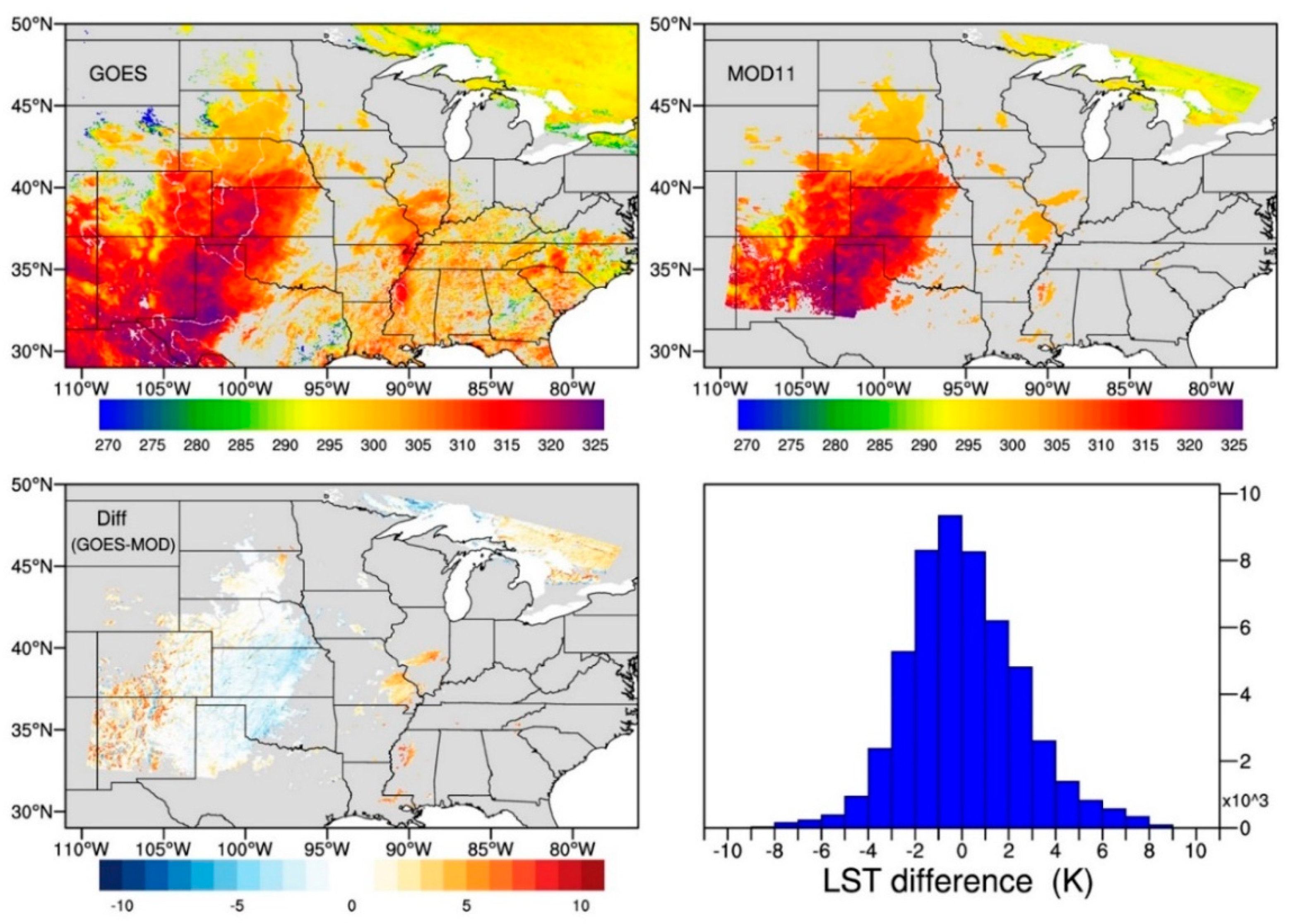
4.2. Evaluation against MOD11

We have conducted an inter-comparison between MOD11_L2 and our LST retrievals. Before comparison, the MOD11_L2 data are rescaled to 0.05 × 0.05 degree latitude/longitude grids.

Figure 4 shows an example of comparison between the GOES_RTTOV LST and MOD11_L2 LST on 11 June 2004 UTC 17:15.

We compared 25 match-up cases for which the two products have overlap and both start scan at 15 min after same hour in 2004. For most cases, the total number of points in the overlap area is more than 40,000. Figure 5 presents the correlation coefficients (corr), the mean bias (bias), the standard deviation (std) and the root mean square error (rmse) between the two products. As seen, in most cases, the two products yield close correlation. Only in one case the coefficient is less than 0.8. The averaged corr of all cases is 0.91. More than 50% cases have mean bias less than 2 K, and the averaged value is 1.7 K. The averaged std and rmse are 2.7 and 3.3 K respectively.

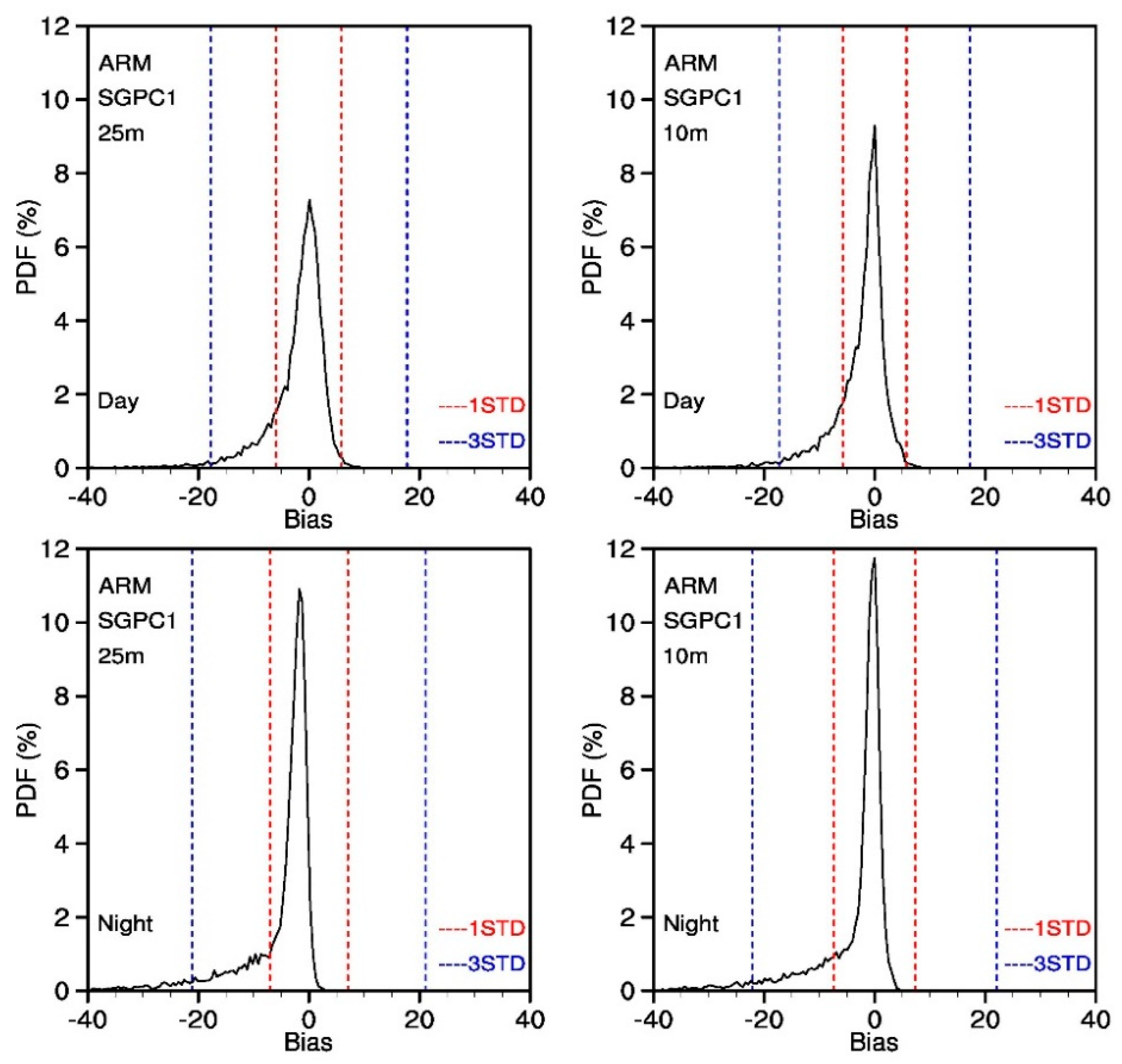
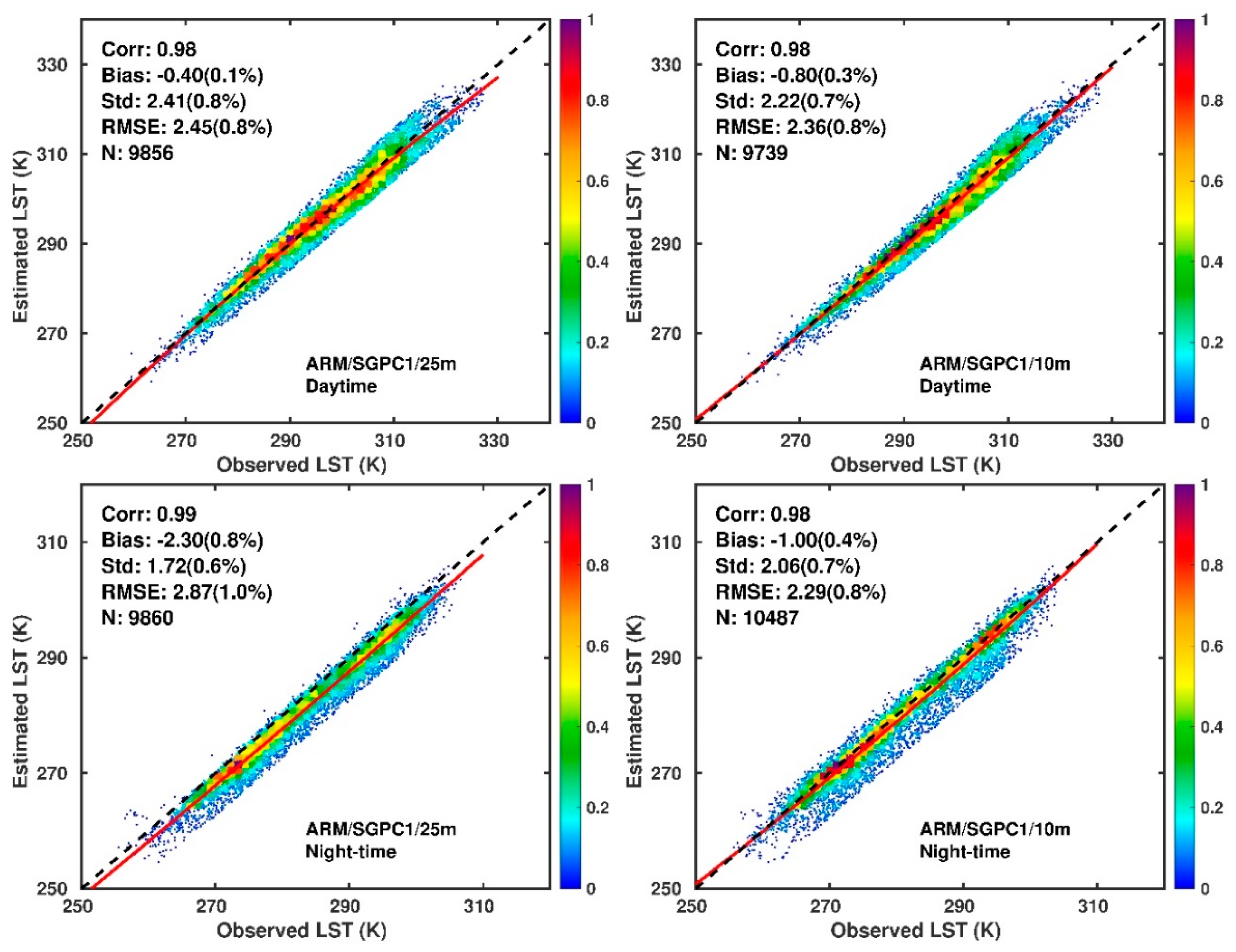
4.3. Evaluation against ARM SGP Site at Instantaneous Time Scale

The IRT data are available from two levels of a tower; one instrument was located at 25 m and one at 10 m above ground. The probability distribution of differences between GOES_RTTOV_LST and ARM IRT is shown in Figure 6 using all available retrievals. Obviously, most of the differences fall within the interval of 1 std. Less than 20% of the cases are beyond 1 std. The correlation between the two data sets is high for both levels, (>than 0.80 for all cases). The mean differences at daytime are smaller than at nighttime at both levels and the same applies to std and rmse. Numerical values for the cases of Figure 6 are shown in

Table 3. Statistical results for cases illustrated in Figure 6.

	Corr		Mean Bias		Std		RMS		No. Cases
	Day	Night	Day	Night	Day	Night	Day	Night	Day	Night
25 m	0.89	0.81	−2.09	−5.12	5.92	7.04	6.28	8.7	11,781	12,335
10 m	0.89	0.80	−2.68	−3.64	5.75	7.37	6.34	8.22	11,940	12,639

. Differences due to the height exposure of the instrument can be caused by differences in the field of view of the instrument, and as such, different shading effects.

Figure 7 shows the results of evaluations for 2004–2009 from tower observations: (a) for daytime from 25 m level; (b) same as (a) using observations from 10 m level (year 2006 excluded since this year requires additional quality control); (c) same as (a) for nighttime observations only; (d) same as (b) for nighttime observations only. Only values within 1 std are used. The satellite product underestimates the ARM IRT observations, yet, the difference between them is less than 1% and the std and rmse are also around 1%; the performance at daytime is better than at nighttime, most likely, due to better cloud detection during the daytime when observations from the visible channel are available.

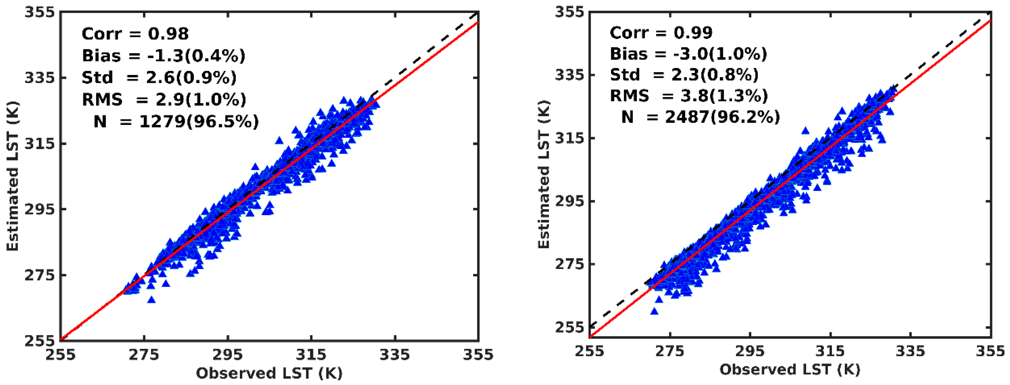
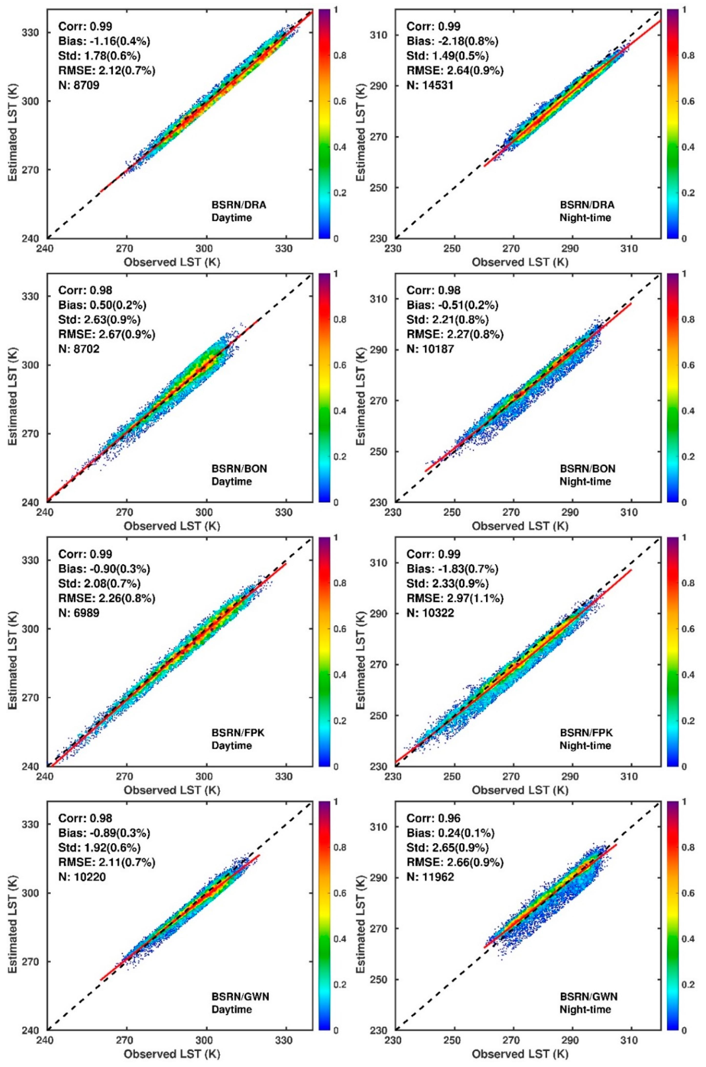
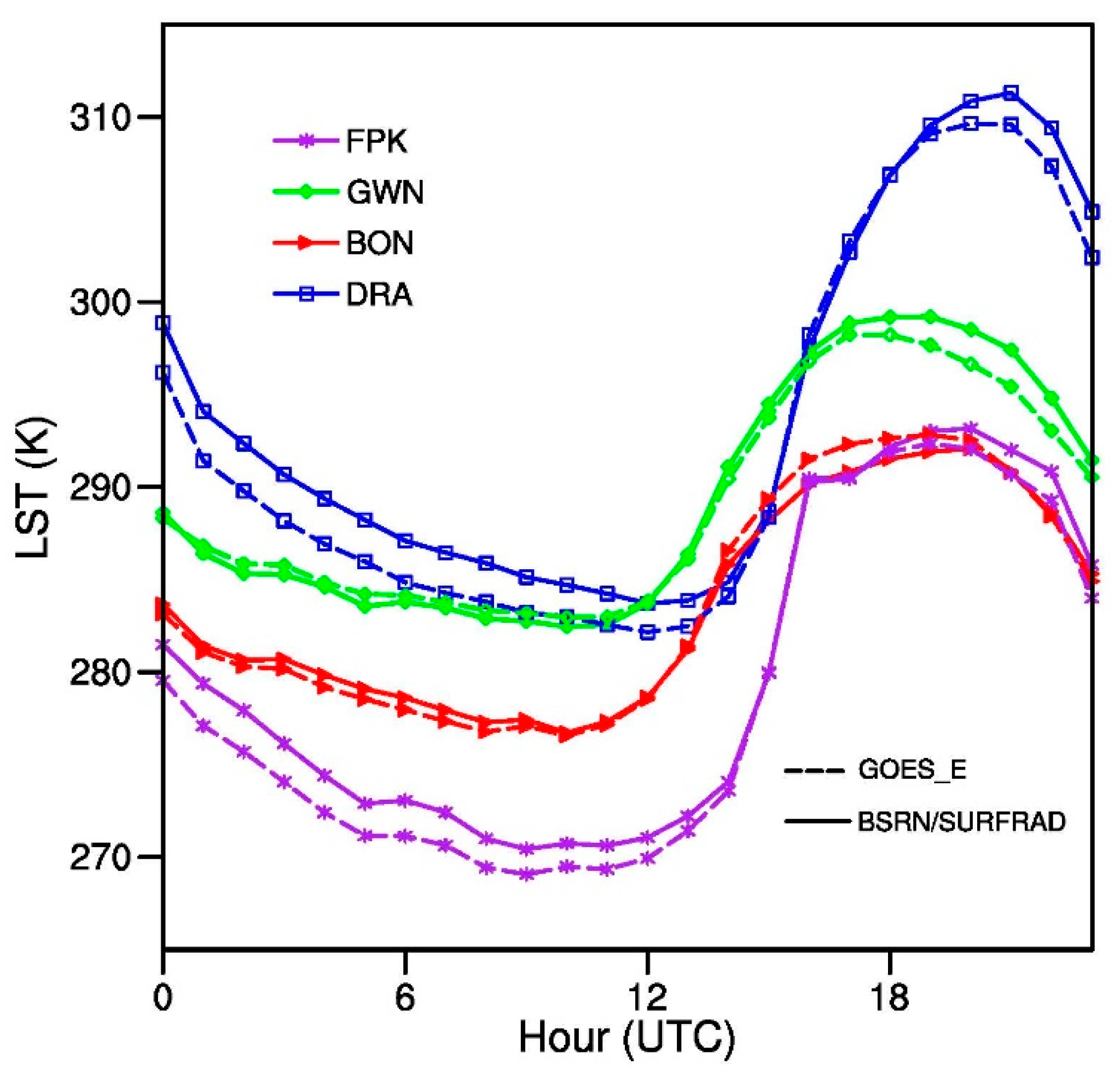
4.4. Evaluation against SURFRAD/BSRN

The SURFRAD/BSRN network observes upwelling (F↑) and down-welling ($F\downarrow$) radiative fluxes which are converted to temperature as follows:

$$F\uparrow ={\epsilon }_{IR}\sigma T_S^4+\left(1-{\epsilon }_{IR}\right)F\downarrow$$

(10)

where ${\epsilon }_{IR}$ is the surface broadband emissivity assigned by surface type, $\sigma$ is the Stefan-Boltzmann constant and is equal to 5.669 × 10⁻⁸ J m⁻²s⁻¹K⁻⁴. Then

$$T_S={\left[\frac{F\uparrow -\left(1-\epsilon \right)F\downarrow }{\epsilon \sigma }\right]}^{1/4}$$

(11)

The approach we use was also applied by others. The main issue in the conversion is the value of emissivity. Heidinger et al. [34] use a broadband longwave emissivity assumed to be 0.97. They indicate that a 0.1 error in emissivity equates to an error in the SURFRAD LST not exceeding 0.25 K. Yu et al. [59] also used the SURFRAD data to evaluate their LST retrievals following the same procedures. In their approach, the emissivity is estimated by mapping surface type classification of Snyder et al. [60] to emissivity (an approach that was popular for some time when direct information on emissivity was not available). They assume that the mean broadband emissivity of the satellite sensor is applicable. We use the CAMEL emissivity which is derived spectrally and integrated to the window spectral interval of the satellite used, and variable at monthly time scale; namely, for each month and for each location the spectral values are integrated to give a new broadband value. This is the most advanced use of surface emissivity in such retrievals.

The scatter plots of the instantaneous GOES_RTTOV LST against SURFRAD sites for both daytime and nighttime are shown in Figure 8. As seen, the satellite estimates and the ground observations have very high correlation, mostly above 0.98. For daytime (left panel Figure 8) the differences ranged between 0.4 (0.2%) to 1.16 (0.4%) while the std ranged between 1.88 (0.6% to 2.53 (0.9%) respectively. For nighttime (right panel Figure 8) the results are comparable to daytime.

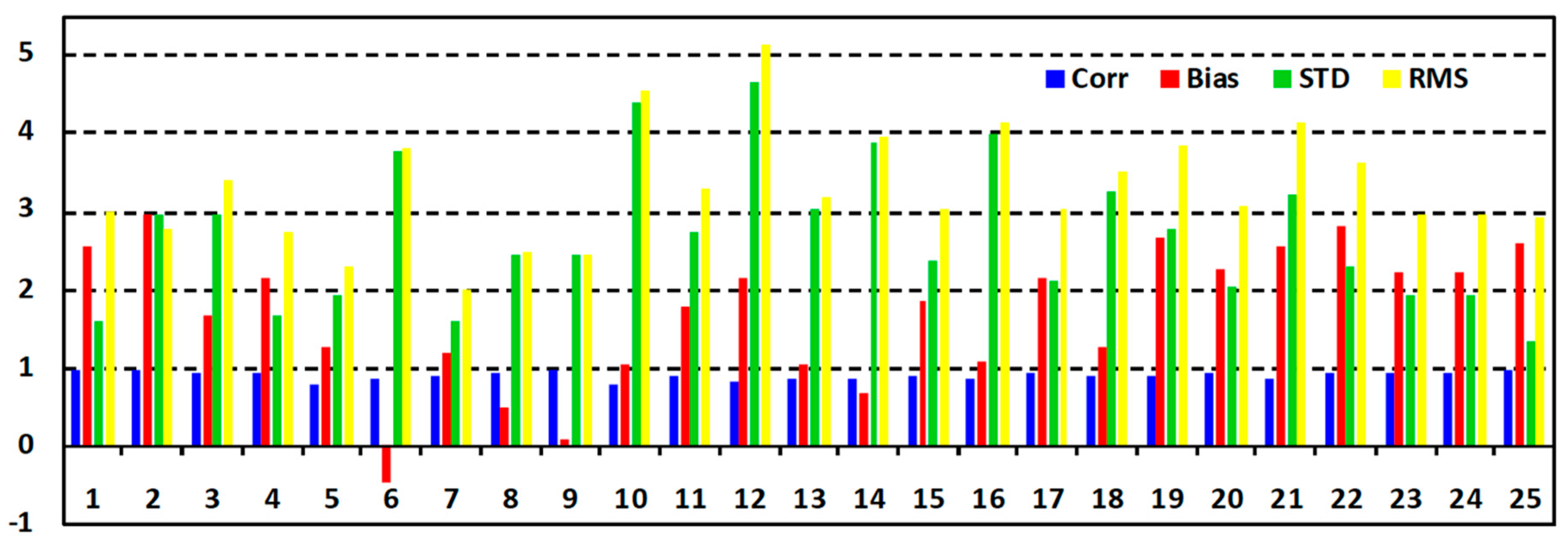
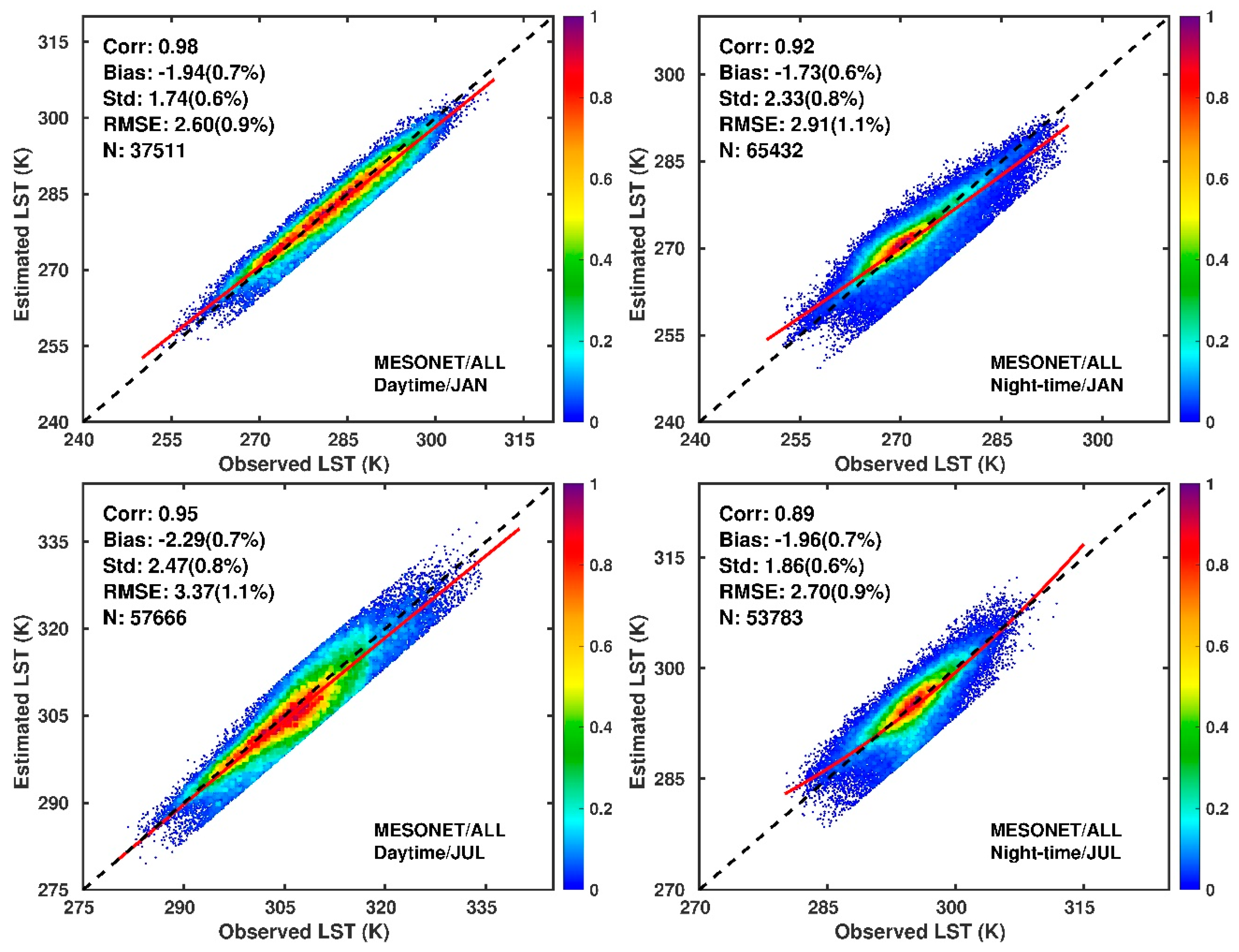
4.5. Evaluation against the Oklahoma MESONET Sites

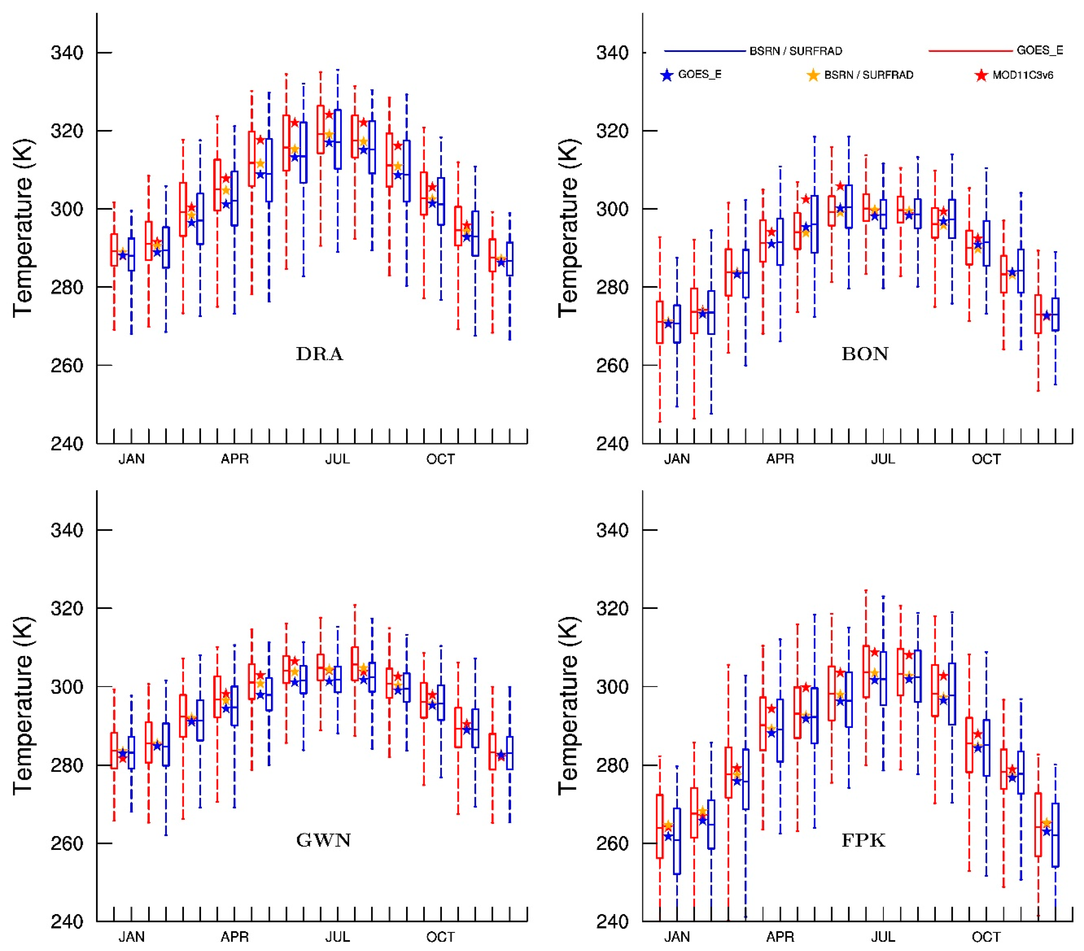
The distribution of sites used in current evaluation is illustrated in Figure 3a. The evaluations are carried out against all the stations for both daytime and nighttime in January and July during 2004–2007. Results are presented in Figure 9 where outliers outside 1 std were removed. Red color designates results that have bias smaller than 1 std, ranging from 1.74 to 2.47 K. The retrieved data have high correlation with the in-situ data (>than 0.9). Results of daytime and nighttime for January and July are comparable (unlike the results of Figure 6 where all outliers were used).

4.6. Applications

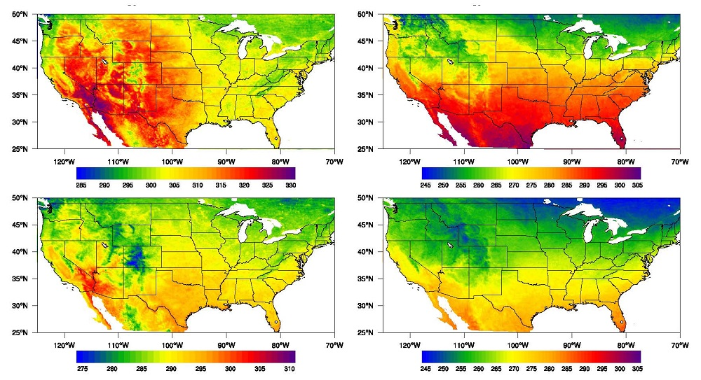
• Seasonal distribution of LST at monthly scale

Since many users of LST data are interested in monthly mean values, we have conducted a comprehensive comparison at such scale. This was possible due to the availability of both ground observations and satellite estimates for a period of six years.

The evaluation was expanded to include ground observations at the USA BSRN/SURFRAD sites and we also used information from MOD11C3, Version: 006 at 0.05° (https://lpdaac.usgs.gov/dataset_discovery/modis/modis_products_table/mod11c3_v006). Derived statistics includes mean values, standard deviation, maximum/minimum, and medium values for each month are shown in Figure 10. It is clearly that the GOES_RTTOV LST has very close distribution pattern as it of SURFRAD/BSRN. It has the ability to describe the annual variability of the LSTs at SURFRAN/BSRN sites. At DRA, MOD11C3v6 LST yields higher estimations against SURFRAD/BSRN for most seasons, the annual mean LST for all study years is 306.6 K, which is 3.1 K higher than the value of SURFRAD/BSRN. While the GOES_RTTOV estimations are much closer to the site value. The annul mean LST of GOES_RTTOV is 301.6 K. For BON, both of the MOD11C3v6 and GOES_RTTOV estimations are close to the site values, except April, May and June. The annul mean LSTs of SUFRAD/BON, GOES_RTTOV and MOD11 are 287.9 K, 288.0 K, 289.8 K respectively. And for GWN, the GOES_RTTOV has relatively lower estimation of annual mean LST which is 293.6 K. The site value is 295.1 K. The MOD11 is 295.7 K. The performance of the satellite estimations at FPK is similar as DRA. The MOD11 annual mean LST is 288.4 K, the GOES_RTTOV is 283.8 K, and the site value is 285.2 K.

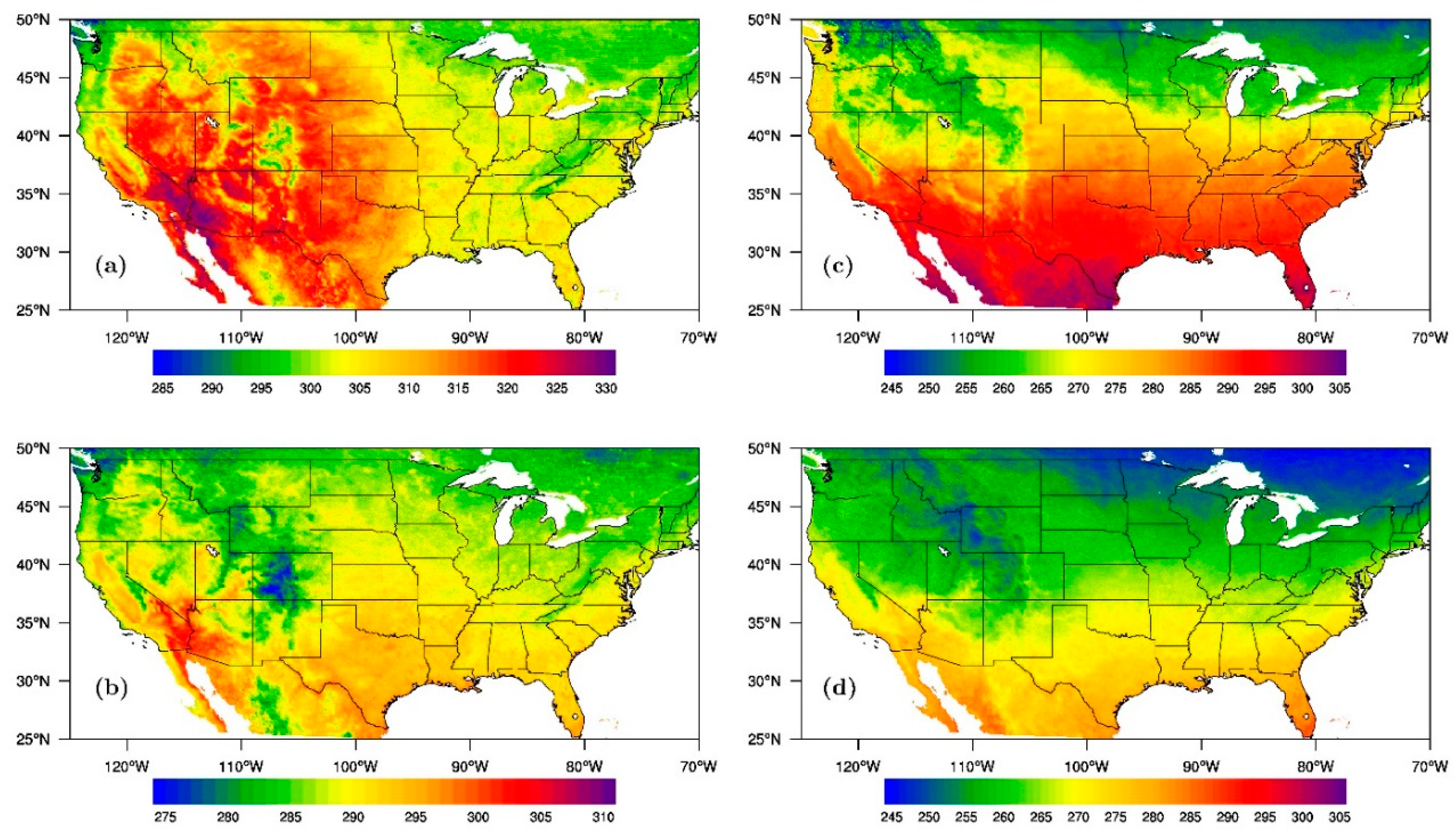
• A six-year climatology of LST over the US

A six year (2004-2009) monthly means of LST at 0.05° spatial resolution for January and July at UTC 06:15 and at UTC 18:15 are shown in Figure 11 for illustration of the product.

As shown, for July, the differences in surface temperature during these two hours (close to representing daily max and min), are large. During the daytime, the western part of the US is dominated by clear sky conditions (the 100th W longitude is known to separate between the humid and dry parts of the US). During the nighttime, the clear conditions contribute to cooling by emitted LW radiation especially, over high elevations. Noticeable is also the pronounced latitudinal variability in the LST during January, dominated by solar zenith angle dependence of heating by SW radiation. The high spatial and temporal resolution of this product makes it useful for addressing hydrological issues such as modeling of evapotranspiration, snow-melt, or soil moisture estimation (utilizing morning heating rates) [61].

In Figure 12 we depict the diurnal variation of LST as observed at four SURFRAD/BSRN stations and from GOES-12. Notable is the large amplitude at the dry site of Desert Rock (DRA) (characterized as desert, gravel, flat, rural) as compared to the more vegetated regions at the other sites (BON is grass, flat, rural; FPK is grass, flat while GWN is grass, hilly, rural). The effect of latitude is also evident. The amplitude at GWN which is at ~34°N is much smaller than the amplitudes at the higher latitude stations (BON at ~40° and FPK at ~48°). Of interest are the differences between satellite estimates and ground observations which are more noticeable at DRA and FPK than at the other sites. A possible explanation for DRA is the lower homogeneity of the site compared to the others. The FPK is at higher elevation than BND and GCM and also at higher latitude so possibly, the cooling of the ground at the observational site may not represent the grid domain. Additional investigation is needed to better understand the behavior at these four sites during the earlier part of the day. The full agreement between the satellite and ground observations from about noon to late afternoon can possibly be due to more even heating of the ground than at the earlier hours of the day when the higher moisture content can differentially affect the emissivity. While ground observations are very sparse, the findings shown in Figure 12 indicate that satellites alone can be used to characterize the diurnal cycle over the domain of the GOES satellites (a comprehensive analysis over the entire US is needed). This information is of considerable interest since most satellite based estimates of LST use polar orbiters unable to depict the true diurnal cycle.

5. Discussion

Available information on LST and DTR from remotely sensed data is deficient. Discrepancies and inconsistencies arise due to the quality of the satellite and the ground observations, differences in their spatial, spectral and temporal resolution, as well as differences in the inference methods and auxiliary data used. In principle, the well-established split window approach is known to perform better than the use of a single channel for deriving LST however, the 12 µm channel is not available any more during the operational period of GOES 12-15. To homogenize satellite observations to obtain a consistent long term record requires the utilization of observations from a single channel only.

With the advancement in archiving of satellite data, their maintenance in terms of calibration, geolocation, improved inference schemes and auxiliary information, it is timely to formulate an approach for deriving long-term, consistent, and calibrated data across multiple satellite sensors, as demanded by the user community. Progress has also been made in ground observations in terms of instrument characterization, guidelines for high quality maintenance and calibration. The issue of optimal coupling between satellite and ground observations is still widely debated.

LST is known to have large spatial variability at different temporal scale (diurnal, annual, inter-annual) and this variability has an informative value. For instance, the importance of the diurnal cycle of LST has been widely recognized [62,63,64] and numerous attempts have been made to estimate it. In an early attempt [65], used were the International Satellite Cloud Climatology Project (ISCCP) data (at 280 km resolution C-2 product) [66] in combination with ground observations to derive the monthly mean diurnal cycle in surface temperature over land (suitable for Global Climate studies). Duan et al. [64] tried to determine it using High Spatial Resolution Clear-Sky MODIS Data while Inamdar et al. [33] dis-aggregated the diurnal cycle of LST at the GOES pixel scale to that of the MODIS pixel scale. Yet, the daytime and nighttime products from polar orbiting satellites (e.g., MODIS) do not fully represent the daily amplitude as feasible from GEO satellites. Our effort represents a contribution to the development of a framework for obtaining long term records of consistent LST and DTR from the entire record of GOES satellites, using a physically based approach and utilizing the best currently available auxiliary information and the best available ground observations to evaluate the proposed approach.

In the evaluation process, factors that play a role include differences in ground instrumentation, their location above the surface, method of estimating LST from the measured outgoing LW radiation, calibration and maintenance of the instruments and scale issues between ground observations and satellite footprints. There is a need to ensure that the satellite observations used represent clear sky condition. Detailed information on each of these factors is needed for a full assessment of errors in the retrieved LST products. While under controlled short term experiments the uncertainty of many of these factors can be minimized, the results obtained are not representative for extended areas and all seasons.

In this paper, the quality of the new product is evaluated against extensive record of best available observations and products that are accepted by the scientific community. Specifically, evaluation of a six-year record of instantaneous LST as well as monthly averages was performed against the DOE Atmospheric Radiation Measurement (ARM) site at the Southern Great Plains central facility, the BSRN/SURFRAD stations, MOD11 products and the Oklahoma MESONET sites.

While the quality of the instrumentation used at each site can be traced to factory specifications, it is not possible to establish how much differences in daily maintenance at each site contribute to the quality of the observations. The hypothesis of our approach is that by using long term observations at numerous sites and seasons, the evaluation results do provide an indication on the robustness of the approach. One of the major factors affecting the evaluation results is related to cloud screening which vary among methodologies as recently discussed in Ermida et al. [67]. Spatial and temporal variability in emissivity are also a contributing factors. As reported in [6] a brightness temperature error due to emissivity error in the 11 µm band is about 3% for a 0.5% error in emissivity and up to 5% for an emissivity error of 2.0%; these estimates are based on global simulations over a wide temperature range. To fully understand discrepancies between products, there is a need in controlled experiments to evaluate independently factors that can cause differences. Till now, available retrievals are based on different satellite observation, different retrieval methodology, atmospheric inputs and time periods. An early attempt to compare the performance of several well-known algorithms was presented in {6]. To make such algorithm comparison consistent the individual methodologies need to be modified; it is necessary to rederive relevant coefficients of the algorithms used in a systematic manner using the same inputs. The need for controlled experiments to facilitate discussion on sources of discrepancies between methods has been recognized by the scientific community and is conducted frequently. Examples are numerical model evaluation as conducted at Lawrence Livermore National Laboratory (https://pcmdi.llnl.gov/?projects/amip/0), while controlled experiments to estimate errors due to aerosols is described in Randles et al. [68]. The objective of the current study is to present a credible methodology to generate long term time series of LST at best available spatial and temporal resolution (that currently are possible with a long term outlook), and evaluate it against best available satellite products and ground observations. Used were long term observations that represent different climatic regions and seasons that provided statistically robust indication on the soundness of the propose approach. The need for further work to investigate the sources of discrepancies is also recognized. Limitations and advantages of each methods and their trade-offs need also to be fully understood.

6. Summary

In principle, the split window approach is known to perform better than a single channel to derive LSTs. But the 12 µm channel is not available any more during the operation periods of GOES 12–15. To homogenize satellite observations to a consistent long term record requires the use of a single channel observation.

We have implemented the RTTOV radiative transfer approach adjusted for GEO channel 4 to derive LST at the high resolution of about 5-km. The model is driven with the MERRA-2 reanalysis profiles for water vapor and temperature and the CAMEL product. A homogeneous six year record of LST at 0.05° spatial resolution at hourly time scale was produced from GOES observations and evaluated for the period of 2004–2009. A six year climatology at monthly time scales was also derived and used to construct representative diurnal cycles for selected surface type.

The results shows that there is a close agreement between the GEO and MOD11 products. The averaged correlation coefficient between them is over 0.9. The averaged difference is less than 2 K and the averaged rmse is less than 3.5 K. It was also found that the derived LST has very close correlation with ground-based observations. In most cases, the correlation coefficients are greater than 0.9. The mean differences between the satellite LST and the station LST are less than 1% and over 80% of the differences fall within 1 std. The performance of retrieved LST for daytime and nighttime are comparable to each other after elimination of outliers caused by imperfect cloud detection. The estimated quality of the LST information can serve as a guideline for users in a wide range of applications, such as a realistic representation of the diurnal cycle.

Future improvement would be possible by satellite observations of higher spatial resolution, the incorporation of higher temporal resolution of surface emissivity and improved/innovative methodologies to remove cloud contamination [68] and by accounting for anisotropy in emissivity Pinheiro et al. [69], Ermida et al. [70].

References

1. Trenberth, K.E.; Stepaniak, D.P.; Caron, J.M. Accuracy of atmospheric energy budgets from analyses. J. Clim. 2002, 15, 3343–3360. [Google Scholar] [CrossRef]
2. Garand, L.; Buehner, M.; Wagneur, N. Background Error Correlation between Surface Skin and Air Temperatures: Estimation and Impact on the Assimilation of Infrared Window Radiances. J. Appl. Met. 2004, 43, 1853–1863. [Google Scholar] [CrossRef]
3. Price, J.C. Estimation of surface temperatures from satellite thermal infrared data—A simple formulation for the atmospheric effect. Remote Sens. Environ. 1983, 13, 353–361. [Google Scholar] [CrossRef]
4. Becker, F.; Li, Z.L. Toward a local split window method over land surface. Int. J. Remote Sens. 1990, 11, 369–393. [Google Scholar] [CrossRef]
5. Wan, Z.M.; Dozier, J. A generalized split-window algorithm for retrieving land-surface temperature from space. IEEE Trans. Geosci. Remote Sens. 1996, 34, 892–905. [Google Scholar] [Green Version]
6. Sun, D.; Pinker, R.T. Estimation of land surface temperature from a Geostationary Operational Environmental Satellite (GOES-8). J. Geophys. Res. 2003, 108, 4326. [Google Scholar] [CrossRef]
7. Sobrino, J.A.; Li, Z.L.; Stoll, M.P.; Becker, F. Improvements in the split window technique for land surface temperature determination. IEEE Trans. Geosci. Remote Sens. 1994, 32, 243–253. [Google Scholar] [CrossRef]
8. Nerry, F.; Labed, J.; Stoll, M.P. Spectral properties of land surfaces in the thermal infrared: 1. Laboratory measurements of absolute spectral emissivity signatures. J. Geophys. Res. 1990, 95, 7027–7044. [Google Scholar] [CrossRef]
9. Hulley, G.C.; Hughes, C.G.; Hook, S.J. Quantifying uncertainties in land surface temperature and emissivity retrievals from ASTER and MODIS thermal infrared data. J. Geophys. Res. 2012, 117, D23113. [Google Scholar] [CrossRef]
10. Lorenz, D. The effect of the long-wave reflectivity of natural surfaces on surface temperature measurements using radiometers. J. Appl. Meteorol. 1986, 5, 421–430. [Google Scholar] [CrossRef]
11. Li, Z.-L.; Tang, B.-H.; Wu, H.; Ren, H.; Yan, G.; Wan, Z.; Trigo, I.F.; Sobrino, J.A. Satellite-derived land surface temperature: Current status and perspectives. Remote Sens. Environ. 2013, 131, 14–37. [Google Scholar] [CrossRef] [Green Version]
12. Prabhakara, C.; Dalu, G.; Kunde, V.G. Estimation of sea surface temperature from remote sensing in the 11- and 13-µm window region. J. Geophys. Res. 1974, 79, 5039–5044. [Google Scholar] [CrossRef]
13. McClain, E.P.; Pichel, W.G.; Walton, C.C.; Ahmad, Z.; Sutton, J. Multichannel improvements to satellite-derived global sea surface temperatures. Adv. Space Res. 1983, 2, 43–47. [Google Scholar] [CrossRef]
14. Becker, F.; Li, Z.-L. Surface temperature and emissivity at various scales: Definition, measurement and related problems. Remote Sens. Rev. 1995, 12, 225–253. [Google Scholar] [CrossRef]
15. McMillin, L.M. Estimation of sea surface temperatures from two infrared window measurements with different absorption. J. Geophys. Res. 1975, 80, 5113–5117. [Google Scholar] [CrossRef]
16. Prata, A.J. Land surface temperatures derived from the advanced very high resolution radiometer and the along-track scanning radiometer: 2. Experimental results and validation of AVHRR algorithms. J. Geophys. Res. 1994, 99, 13025–13058. [Google Scholar] [CrossRef]
17. François, C.; Ottlé, C. Atmospheric corrections in the thermal infrared: Global and water vapor dependent split-window algorithms-applications to ATSR and AVHRR data. IEEE Trans. Geosci. Remote Sens. 1996, 34, 457–470. [Google Scholar] [CrossRef]
18. Coll, C.; Caselles, V.; Galve, J.M.; Valor, E.; Niclòs, R.; Sanchez, J.M. Ground measurements for the validation of land surface temperatures derived from AATSR and MODIS data. Remote Sens. Environ. 2005, 97, 288–300. [Google Scholar] [CrossRef]
19. Trigo, I.F.; Monteiro, I.T.; Olesen, F.; Kabsch, E. An assessment of remotely sensed land surface temperature. J. Geophys. Res. 2008, 113, D17108. [Google Scholar] [CrossRef]
20. Wan, Z. New refinements and validation of the collection-6 MODIS land-surface temperature/emissivity product. Remote Sens. Environ. 2014, 140, 36–45. [Google Scholar] [CrossRef]
21. Van de Griend, A.A.; Owe, M. On the relationship between thermal emissivity and the normalized difference vegetation index for natural surfaces. Int. J. Remote Sens. 1993, 14, 1119–1131. [Google Scholar] [CrossRef]
22. Valor, E.; Caselles, V. Mapping land surface emissivity from NDVI: Application to European, African, and South American areas. Remote Sens. Environ. 1996, 57, 167–184. [Google Scholar] [CrossRef]
23. Karnieli, A.; Agam, N.; Pinker, R.T.; Anderson, M.; Imhoff, M.I.; Gutman, G.G.; Panov, N.; Goldberg, A. Use of NDVI and LST for Assessing Vegetation Health: Merits and Limitations. J. Clim. 2010, 23, 618–633. [Google Scholar] [CrossRef]
24. Kealy, P.S.; Hook, S.J. Separating temperature and emissivity in thermal infrared multispectral scanner data: Implications for recovering land surface temperatures. IEEE Trans. Geosci. Remote Sens. 1993, 31, 1155–1164. [Google Scholar] [CrossRef]
25. Gillespie, A.; Rokugawa, S.; Matsunaga, T.; Cothern, J.S.; Hook, S.; Kahle, A.B. A temperature and emissivity separation algorithm for Advanced Spaceborne Thermal Emission and Reflection Radiometer (ASTER) images. IEEE Trans. Geosci. Remote Sens. 1998, 36, 1113–1126. [Google Scholar] [CrossRef]
26. Wan, Z.; Li, Z.-L. A physics-based algorithm for retrieving land-surface emissivity and temperature from EOS/MODIS data. IEEE Trans. Geosci. Remote Sens. 1997, 35, 980–996. [Google Scholar]
27. Liang, S. An optimization algorithm for separating land surface temperature and emissivity from multispectral thermal infrared imagery. IEEE Trans. Geosci. Remote Sens. 2001, 39, 264–274. [Google Scholar] [CrossRef]
28. Schmugge, T.; French, A.; Ritchie, J.C.; Rango, A.; Pelgrum, H. Temperature and emissivity separation from multispectral data. Remote Sens. Environ. 2001, 78, 189–198. [Google Scholar]
29. Ma, X.L.; Wan, Z.; Moeller, C.C.; Menzel, W.P.; Gumley, L.E. Simultaneous retrieval of atmospheric profiles, land-surface temperature, and surface emissivity from Moderate-Resolution Imaging Spectroradiometer thermal infrared data: Extension of a two-step physical algorithm. Appl. Opt. 2002, 41, 909–924. [Google Scholar] [CrossRef] [PubMed]
30. Borbas, E.; Hulley, G.; Feltz, M.; Knuteson, R.; Hook, S. The Combined ASTER MODIS Emissivity over Land (CAMEL) Part 1: Methodology and High Spectral Resolution Application. Remote Sens. 2018, 10, 643. [Google Scholar] [CrossRef]
31. Feltz, M.; Borbas, E.; Knuteson, R.; Hulley, G.; Hook, S. The Combined ASTER MODIS Emissivity over Land (CAMEL) Part 2: Uncertainty and Validation. Remote Sens. 2018, 10, 664. [Google Scholar] [CrossRef]
32. Sun, D.; Pinker, R.T. Implementation of GOES-based land surface temperature diurnal cycle to AVHRR. Int. J. Remote Sens. 2005, 26, 3975–3984. [Google Scholar] [CrossRef]
33. Inamdar, A.K.; French, A.; Hook, S.; Vaughan, G.; Luckett, W. Land surface temperature retrieval at high spatial and temporal resolutions over the southwestern United States. J. Geophys. Res. 2008, 113, D07107. [Google Scholar] [CrossRef]
34. Heidinger, A.K.; Evan, A.T.; Foster, M.J.; Walther, A. A naive Bayesian cloud detection scheme derived from CALIPSO and applied with PATMOS-x. J. Appl. Meteorol. Climatol. 2012, 51, 1129–1144. [Google Scholar] [CrossRef]
35. Scarino, B.R.; Minnis, P.; Chee, T.; Bedka, K.M.; Yost, C.R.; Palikonda, R. Global clear-sky surface skin temperature from multiple satellites using a single-channel algorithm with angular anisotropy corrections. Atmos. Meas. Tech. 2017, 10, 351–371. [Google Scholar] [CrossRef] [Green Version]
36. Gunshor, M.M.; Schmit, T.J.; Menzel, W.P.; Tobin, D.C. Intercalibration of broadband geostationary imagers using AIRS. J. Atmos. Ocean. Technol. 2009, 26, 746–758. [Google Scholar] [CrossRef]
37. Weinreb, M.P.; Jamieson, M.; Fulton, N.; Chen, Y.; Johnson, J.X.; Bremer, J.; Smith, C.; Baucom, J. Operational calibration of geostationary operational environmental Satellite-8 and-9 imagers and sounders. Appl. Opt. 2007, 36, 6895–6904. [Google Scholar] [CrossRef]
38. Gelaro, R.; McCarty, W.; Suárez, M.J.; Todling, R.; Molod, A.; Takacs, L.; Randles, C.A.; Darmenov, A.; Bosilovich, M.G.; Reichle, R.; et al. The Modern-Era Retrospective Analysis for Research and Applications, Version 2 (MERRA-2). J. Clim. 2017, 30, 5419–5454. [Google Scholar] [CrossRef]
39. Wan, Z. MODIS Land Surface Temperature Products Users’ Guide; Collection-6, ERI; University of California: Santa Barbara, CA, USA, 2013. [Google Scholar] [CrossRef]
40. Hicks, B.B.; DeLuisi, J.J.; Matt, D.R. The NOAA Integrated Surface Irradiance Study (ISIS)—A new surface radiation monitoring program. Bull. Am. Meteorol. Soc. 1996, 77, 2857–2864. [Google Scholar] [CrossRef]
41. Ohmura, A.; Dutton, E.G.; Forgan, B.; Fröhlich, C.; Gilgen, H.; Hegner, H.; Heimo, A.; König-Langlo, G.; McArthur, B.; Müller, G.; et al. Baseline Surface Radiation Network (BSRN/WCRP): New precision radiometry for climate research. Bull. Am. Meteorol. Soc. 1998, 79, 2115–2136. [Google Scholar] [CrossRef]
42. Augustine, J.A.; Hodges, G.B.; Cornwall, C.R.; Michalsky, J.J.; Medina, C.I. An update on SURFRAD: The GCOS surface radiation budget network for the continental United States. J. Atmos. Ocean. Technol. 2005, 22, 1460–1472. [Google Scholar] [CrossRef]
43. Guillevic, P.; Göttsche, F.; Nickeson, J.; Hulley, G.; Ghent, D.; Yu, Y.; Trigo, I.; Hook, S.; Sobrino, J.A.; Remedios, J.; et al. Land Surface Temperature Product Validation Best Practice Protocol, Version 1.0. In Best Practice for Satellite-Derived Land Product Validation (p. 60): Land Product Validation Subgroup (WGCV/CEOS); Guillevic, P., Göttsche, F., Nickeson, J., Román, M., Eds.; Internal Publication: Brussels, Belgium, 2017. [Google Scholar] [CrossRef]
44. McPherson, R.A.; Fiebrich, C.A.; Crawford, K.C.; Kilby, J.R.; Grimsley, D.L.; Martinez, J.E.; Basara, J.B.; Illston, B.G.; Morris, D.A.; Kloesel, K.A.; et al. Statewide monitoring of the mesoscale environment: A technical update on the Oklahoma Mesonet. J. Atmos. Ocean. Technol. 2007, 24, 301–321. [Google Scholar] [CrossRef]
45. Fiebrich, C.A.; Martinez, J.E.; Brotzge, J.A.; Basara, J.B. The Oklahoma Mesonet’s skin temperature network. J. Atmos. Ocean. Technol. 2003, 20, 1496–1504. [Google Scholar] [CrossRef]
46. Fuchs, M. Infrared measurement of canopy temperature and detection of plant water stress. Theor. Appl. Climatol. 1990, 42, 253–261. [Google Scholar] [CrossRef]
47. Sobrino, J.A.; Skokovic, D. Permanent Stations for Calibration/Validation of Thermal Sensors over Spain. Data 2016, 1, 10. [Google Scholar] [CrossRef]
48. Hansen, M.C.; Defries, R.S.; Townshend, J.R.G.; Sohlberg, R. Global land cover classification at 1 km resolution using a classification tree approach. Int. J. Remote Sens. 1998, 21, 1331–1364. [Google Scholar] [CrossRef]
49. Li, X.; Pinker, R.T.; Wonsick, M.M.; Ma, Y. Toward improved satellite estimates of short-wave radiative fluxes-Focus on cloud detection over snow: 1. Methodology. J. Geophys. Res. 2007, 112, D07208. [Google Scholar] [CrossRef]
50. Pinker, R.T.; Li, X.; Meng, W.; Yegorova, E.A. Toward improved satellite estimates of short-wave radiative fluxes-Focus on cloud detection over snow: 2. Results. J. Geophys. Res. 2007, 112, D09204. [Google Scholar] [CrossRef]
51. Wang, H.; Pinker, R.T.; Minnis, P.; Khaiyer, M.M. Experiments with Cloud Properties: Impact on Surface Radiative Fluxes. J. Atmos. Ocean. Technol. 2008, 25, 1034–1040. [Google Scholar] [CrossRef]
52. Miller, S.D. Physical decoupling of the GOES daytime 3.9 µm channel thermal emission and solar reflection components using total solar eclipse data. Int. J. Remote Sens. 2001, 22, 9–34. [Google Scholar] [CrossRef]
53. Eyre, J.R. A Fast Radiative Transfer Model. for Satellite Sounding System; ECMWF Research Department Technical Memorandum 176; European Centre for Medium-Range Weather Forecasts: Reading, UK, 1991. [Google Scholar]
54. Saunders, R.W.; Matricardi, M.; Brunel, P. An Improved Fast Radiative Transfer Model for Assimilation of Satellite Radiance Observations. QJRMS 1991, 125, 1407–1425. [Google Scholar] [CrossRef]
55. Matricardi, M.; Saunders, R. Fast radiative transfer model for simulation of infrared atmospheric sounding interferometer radiances. Appl. Opt. 1999, 38, 5679–5691. [Google Scholar] [CrossRef] [PubMed]
56. Hulley, G.; Freepartner, R.; Malakar, N.; Sarkar, S. Moderate Resolution Imaging Spectroradiometer (MODIS) Land Surface Temperature and Emissivity Product (MOD21) Users’ Guide; Collection-6; Jet Propulsion Laboratory California Institute of Technology: Pasadena, CA, USA, 2016. [Google Scholar]
57. Göttsche, F.; Olesen, F.S.; Høyer, J.L.; Wimmer, W.; Nightingale, T. Fiducial Reference Measurements for Validation of Surface Temperature from Satellites (FRM4STS); Technical Report 3—A Framework to Verify the Field Performance of TIR FRM; ESA Contract No. 4000113848_15I-LG; Internal Publication: Brussels, Belgium, 2017; pp. 1–75. [Google Scholar]
58. Hulley, G.C.; Hook, S.J. Generating Consistent Land Surface Temperature and Emissivity Products between ASTER and MODIS Data for Earth Science Research. IEEE Trans. Geosci. Remote Sens. 2011, 49, 1304–1315. [Google Scholar] [CrossRef]
59. Yu, Y.; Privette, J.P.; Pinheiro, A.C. Evaluation of split-window land surface temperature algorithms for generating climate data records. IEEE Trans. Geosci. Remote Sens. 2008, 46, 179–192. [Google Scholar] [CrossRef]
60. Snyder, W.; Wan, Z.; Zhang, Y.; Feng, Y. Classification based emissivity for land surface temperature measurement from space. Int. J. Remote Sens. 1998, 19, 2753–2774. [Google Scholar] [CrossRef]
61. Zhang, D.; Tang, R.; Zhao, W.; Tang, B.; Wu, H.; Shao, K.; Li, Z.-L. Surface Soil Water Content Estimation from Thermal Remote Sensing based on the Temporal Variation of Land Surface Temperature. Remote Sens. 2014, 6, 3170–3187. [Google Scholar] [CrossRef] [Green Version]
62. Dai, A.; Trenberth, K.E. The diurnal cycle and its depiction in the Community Climate System Model. J. Clim. 2004, 17, 930–951. [Google Scholar] [CrossRef]
63. Aires, F.; Prigent, C.; Rossow, W.B. Temporal interpolation of global surface skin temperature diurnal cycle over land under clear and cloudy conditions. J. Geophys. Res. 2004, 109, D04313. [Google Scholar] [CrossRef]
64. Duan, S.-B.; Li, Z.-L.; Tang, B.-H.; Wu, H.; Tang, R.; Bi, Y.; Zhou, G. Estimation of Diurnal Cycle of Land Surface Temperature at High Temporal and Spatial Resolution from Clear-Sky MODIS Data. Remote Sens. 2014, 6, 3247–3262. [Google Scholar] [CrossRef] [Green Version]
65. Ignatov, A.; Gutman, G. Monthly mean diurnal cycles in surface temperature over and land for global climate studies. J. Clim. 1999, 12, 1900–1910. [Google Scholar] [CrossRef]
66. Rossow, W.B.; Schiffer, R.A. ISCCP Cloud Data Products. Bull. Am. Meteorol. Soc. 1991, 72, 2–20. [Google Scholar] [CrossRef]
67. Randles, C.A.; Kinne, S.; Myhre, G.; Schulz, M.; Stier, P.; Fischer, J.; Doppler, L.; Highwood, E.; Ryder, C.; Harris, B.; et al. Intercomparison of shortwave radiative transfer schemes in global aerosol modeling: Results from the AeroCom Radiative Transfer Experiment. Atmos. Chem. Phys. 2013, 13, 2347–2379. [Google Scholar] [CrossRef]
68. Ermida, S.L.; Trigo, I.S.; DaCamara, C.C.; Jiménez, C.; Prigent, C. Quantifying the Clear-Sky Bias of Satellite Land SurfaceTemperature Using Microwave-Based Estimates. J. Geophys. Res. 2019, 124, 844–857. [Google Scholar] [CrossRef]
69. Pinheiro, A.C.T.; Jeffrey, L. Privette, and Pierre Guillevic, Modeling the Observed Angular Anisotropy of Land Surface Temperature in a Savanna. IEEE Trans. Geosci. Remote Sens. 2006, 44, 1036–1047. [Google Scholar] [CrossRef]
70. Ermida, S.L.; Trigo, I.S.; DaCamara, C.C.; Pires, A.C. A Methodology to Simulate LST Directional Effects Based on Parametric Models and Landscape Properties. Remote Sens. 2018, 10, 1114. [Google Scholar] [CrossRef]
Figure 1. Evaluation of LST for 2004 against a SURFRAD/BSRN station at Desert Rock, NV (DRA) for: Left: daytime; Right: nighttime.
Remotesensing 11 01399 g001
Figure 2. Flow-chart describing the derivation of LST from GOES observations.
Remotesensing 11 01399 g002
Figure 3. (a) Spatial characterization of the sites used in evaluation of the LST products in terms of emissivity as obtained at 1 km spatial resolution using the ASTER Global Emissivity Dataset 1 km V003. (b) Frequency distribution of the emissivity values over sites used in evaluation as illustrated in Figure 3a.
Remotesensing 11 01399 g003
Figure 4. Example case of GOES_RTTOV_LST, MOD11_L2 LST and their difference and its distribution at 11 June 2004 UTC 17:15.
Remotesensing 11 01399 g004
Figure 5. Evaluation of 25 instantaneous match-ups of LST retrievals from GOES observations against MOD11_L2. The x-axis provides the numbering of the cases while the y-axis indicates the correlation (in blue) and the other variables in W/m2.
Remotesensing 11 01399 g005
Figure 6. Probability distribution of differences between the GOES_RTTOV and ARM SGP C1 LST. Red dot line: 1 std; Blue dot line: 3 std.
Remotesensing 11 01399 g006
Figure 7. Evaluation of RTTOV based estimates from GOES-E at the SGPC1 ARM test site using observations at hourly intervals during 2004–2009 for daytime and nighttime from 25 m and 10m tower level. Data that have differences of less than one std were used.
Remotesensing 11 01399 g007
Figure 8. Evaluation of instantaneous GOES based LST estimates at hourly intervals against 4 SURFRAD/BSRN stations, independently for daytime (left panel) and nighttime (right panel) using observations from 2004–2009.
Remotesensing 11 01399 g008
Figure 9. Evaluation of instantaneous GOES based LST estimates at hourly intervals against the MESONET stations, independently for daytime (left panel) and nighttime (right panel) using observations for years 2004–2007.
Remotesensing 11 01399 g009
Figure 10. Daytime LST Distribution of GOES_RTTOV, SURFRAD/BSRN sites over 2004–2009 for each month and their monthly mean values compared with MOD11C3v6. Top/Bottom of dashed line: maxi/min LST; Solid “-”: medium LST: Solid box: quartile of LST. Stars are monthly mean LST of SURFRAD/BSRN sites (orange), GOES_RTTOV (blue) and MOD11C3v6 (red).
Remotesensing 11 01399 g010
Figure 11. Monthly mean LST at 0.05° spatial resolution averaged over 6 years (2004–2009) for January and July; (a) UTC18:15, July; (b) UTC06:15:00, July; (c) UTC18:15, January; (d) UTC06:15, January.
Remotesensing 11 01399 g011
Figure 12. A six-year average (2004–2009) of the hourly LST at four SURFRAD/BSRN stations as observed (solid line) and as derived from the GOES observations (broken line).
Remotesensing 11 01399 g012