The Characteristics of Surface Albedo Change Trends over the Antarctic Sea Ice Region during Recent Decades


Chinese Antarctic Center of Surveying and Mapping, Wuhan University, Wuhan 430079, China
*
Author to whom correspondence should be addressed.
Remote Sens. 2019, 11(7), 821; https://doi.org/10.3390/rs11070821
Submission received: 31 January 2019
/
Revised: 31 March 2019
/
Accepted: 3 April 2019
/
Published: 5 April 2019
(This article belongs to the Section Environmental Remote Sensing)
Abstract
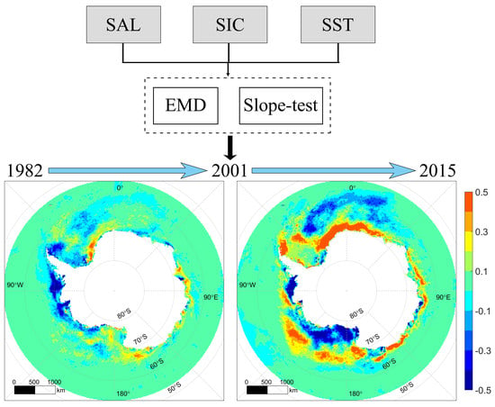
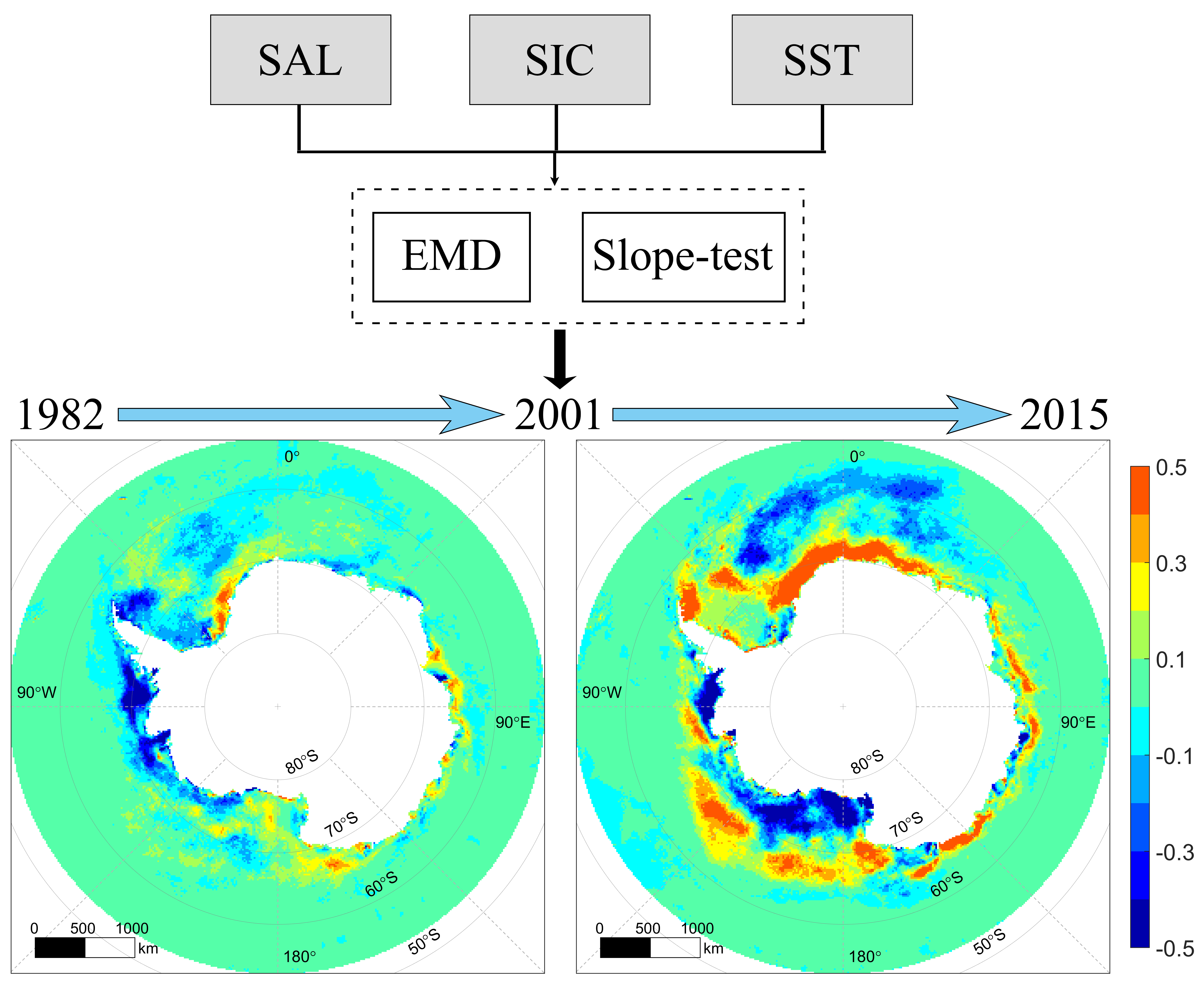
:Based on a long-time series (1982–2015) of remote sensing data, we analyzed the change in surface albedo (SAL) during summer (from December to the following February) for the entire Antarctic Sea Ice Region (ASIR) and five longitudinal sectors around Antarctica: (1). the Weddell Sea (WS), (2). Indian Ocean, (3). Pacific Ocean (PO), (4). Ross Sea, and (5). Bellingshausen–Amundsen Sea (BS). Empirical mode decomposition was used to extract the trend of the original signal, and then a slope test method was utilized to identify a transition point. The SAL provided by the CM SAF cloud, Albedo, and Surface Radiation dataset from AVHRR data-Second Edition was validated at Neumayer station. Sea ice concentration (SIC) and sea surface temperature (SST) were also analyzed. The trend of the SAL/SIC was positive during summer over the ASIR and five longitudinal sectors, except for the BS (−2.926% and −4.596% per decade for SAL and SIC, correspondingly). Moreover, the largest increasing trend of SAL and SIC appeared in the PO at approximately 3.781% and 3.358% per decade, respectively. However, the decreasing trend of SAL/SIC in the BS slowed down, and the increasing trend of SAL/SIC in the PO accelerated. The trend curves of the SST exhibited a crest around 2000–2005; thus, the slope lines of the SST showed an increasing–decreasing type for the ASIR and the five longitudinal sectors. The evolution of summer albedo decreased rapidly in the early summer and then maintained a relatively stable level for the whole ASIR. The change of it mainly depended on the early melt of sea ice during the entire summer. The change of sea ice albedo had a narrow range when compared with composite albedo and SIC over the five longitudinal sectors and reached a stable level earlier. The transition point of SAL/SIC in several sectors appeared around the year 2000, whereas that of the SST for the entire ASIR occurred in 2003–2005. A high value of SAL/SIC and a low value of the SST existed in the WS which can be displayed by the spatial distribution of pixel average. In addition, the lower the latitude was, the lower the SAL/SIC and the higher the SST would be. A transition point of SAL appeared in 2001 in most areas of West Antarctica. This transition point could be illustrated by anomaly maps. The spatial distribution of the pixel-based trend of SAL demonstrated that the change in SAL in East Antarctica has exhibited a positive trend in recent decades. However, in West Antarctica, the change of SAL presented a decreasing trend before 2001 and transformed into an increasing trend afterward, especially in the east of the Antarctic Peninsula.
1. Introduction
Antarctica is sensitive to climate change despite its isolation from human beings [1,2]. Interestingly, the Antarctic is also known as an “indicator” of global climate change [3]. One of the deepest warming rates on Earth has been recorded in the Antarctic Peninsula (with an increase of 0.056 °C per year since 1950) which was reported by Turner et al. (2005) [4]. The recent results of Turner et al. (2016) indicated that this trend has weakened in recent years [5]. However, several works have presented preliminary evidence that the warming trend has slowed down since the beginning of the 21st century, and a cooling trend has occurred in the recent two decades [6,7,8,9]. The variations in sea ice in Antarctica have played a key role in climate changes [10,11,12,13]. Therefore, to improve our understanding of the climate change, we must analyze the changes in the Antarctic sea ice in recent decades.
The changes in Antarctic sea ice considerably affect the change in climate over Antarctica [14,15,16,17]. The increased absorption of sunlight through the earth–atmosphere system results in increasing temperature and the warming of the ocean, thereby further causing a decrease in the sea ice extent and surface albedo (SAL). This effect is called ice–albedo feedback [18,19,20]. The Arctic sea ice is becoming thin and young, whereas the sea ice extent in Antarctica has slightly increased over the last four decades [21,22,23]. Parkinson et al. (2012) used satellite passive–microwave data and found a substantial increasing trend (17100 ± 2300 km2 year−1) of sea ice extent over Antarctica from 1978 to 2010 [24]. Turner et al. (2016) determined an increasing trend by 195 × 103 km2 per decade for the total Antarctic sea ice extent from 1979 to 2013 [25]. However, on the basis of the transition of the Interdecadal Pacific Oscillation from the positive to the negative phases around the year 2000, Meehl et al. (2016) reported that the Antarctic sea ice extent during summer showed a slightly decreasing trend before the 2000s and a considerable increasing trend afterward [7]. De Santis et al. (2017) analyzed the variability and trend of satellite-derived Antarctic sea ice extent from 1979 to 2016 and discovered an increasing trend of 1.6 ± 0.4% per decade [21]. Then, the satellite-derived sea ice extent during 1979 to 2015 was studied by Jena et al. (2018) who declared that the increasing trend of sea ice extent in the Indian Ocean was about 2.4 ± 1.2% per decade [9]. Thus, understanding the changes in sea ice in the Antarctic sea ice region (ASIR) is essential to global climate research.
The albedo, an important factor that affects the radiation balance of the earth–atmosphere system, has frequently been used for research on global climate change [26,27,28]. Given the high albedo of snow and ice surfaces, most of the solar radiation on the surface of snow and ice in the ASIR are reflected back to the atmosphere [29,30,31]. The albedo of unfrozen ocean is between 5% and 20% and is affected by solar zenith angle. Snow/ice albedo, which is strongly dependent on incident solar irradiance, snow grain size, and soot content, ranges from 50% to 90%, and fresh snow albedo reaches 90% [32]. However, substantial incident solar radiation is absorbed by the Antarctic sea ice during summer; thus, the physical state of the snow/ice surface changes rapidly, such that the melting of snow and ice leads to dramatic changes in snow/ice surface albedo [33,34]. A suitable albedo parameterization of ASIR is crucial for the assessment of ice-albedo feedback in Antarctic climate change [35,36]. For ASIR, the composite albedo is estimated using the area fractions and albedos of sea ice and open water. Because the albedo of open water is very small [32], the albedo of sea ice is the key variable of the parameterization of the composite albedo. Therefore, studying the change in albedo is one step in understanding the variation of sea ice and recognizing the trend of climate change in Antarctica.
The Antarctic albedo has been extensively studied owing to its important relationship with climate change. On the basis of SAL data from several Antarctic sites, Pirazzini (2004) indicated that the albedo variability is remarkably correlated with snow/ice metamorphism [27]. Brandt et al. (2005) utilized three ship-based field experiments and measured spectral albedos at ultraviolet, visible, and near-infrared wavelengths for open water, grease ice, nilas, young “gray” ice, young gray-white ice, and first-year ice, with and without snow cover [37]. Data from Advanced Very High-Resolution Radiometer (AVHRR) Polar Pathfinder (APP) product was used by Laine (2007) to analyze the changes in albedo in the Antarctic ice sheet and sea ice region from 1981 to 2000 [38]. Shao et al. (2015) used a dataset consisting of 28 years of homogenized satellite data to calculate the spring–summer albedo of the entire ASIR [39]. Using the Satellite Application Facility on Climate Monitoring (CM SAF) in the European Organisation for Exploitation of Meteorological Satellite “The CM SAF Cloud, Albedo, and Surface Radiation dataset from AVHRR data”—first edition (CLARA-A1) product, Seo et al. (2016) analyzed the temporal and spatial variabilities of albedo over the Antarctic ice sheet [40,41].
Climate change detection is one of the core issues in climate change research, and it plays a crucial role in accurately estimating global and regional climate change trends [42]. Conventionally, linear regression [38], least squares [43], moving average [3] and polynomial [44] are used for trend estimation in climate change research and for many studies of sea ice, particularly in the Polar Regions. In fact, climate change presents a complex nonlinear trend, and most long-term variations in many climatic factors, such as albedo and temperature, show nonlinear and non-stationary complex processes of change [45,46]. Therefore, a variety of scales or periodic climate factors changes are hidden due to the limitation of the conventional methods. To analyze nonlinear and non-stationary data, Huang et al. (1998) proposed a new time series signal processing method: the empirical mode decomposition (EMD), which has strong self-adaptability and local variation characteristics based on the signal [47]. The core idea of the EMD is the so called Hilbert-Huang transform, in which any complicated signal can be decomposed into finite numbers of ‘intrinsic mode functions’ (IMFs) and a residual mode: long-term trend. Compared with conventional methods, it can extract long-term trends of changes in climate factors more efficiently [48]. Shu et al. (2012) used the EMD method to analyze the change in sea ice in Antarctica and found that the rate of increased trend of sea ice has been accelerating in the past decade [49]. By decomposing the long-term (from February 1947 to January 2011) temperature data observed at Faraday/Vernadsky station using EMD, Franzke (2013) demonstrated that most of the temperature variability occurred on intraannual time scales [50]. By using the EMD method, the cyclic and non-cyclic components of sea level change were separated by Galassi and Spada (2017) [51]. Furthermore, the EMD method has been gradually applied in the field of climate change research, and some significant results have been achieved [52,53,54].
In this study, we aim to analyze the SAL of sea ice in recent decades (1982–2015) and investigate climate change over the ASIR. Considering the Antarctic polar night phenomenon, we only analyze the changes in albedo during summer (December to the following February); these changes also contain interesting albedo variations. To study the regional features of climate change over the ASIR, the region is divided into five longitudinal sectors around Antarctica [37,55]. Empirical mode decomposition (EMD) is applied to the SAL, sea ice concentration (SIC), and sea surface temperature (SST) to extract the residual component, which represents their change trend. Then, we use a slope-test method to identify the transition point. After the time series and trend analysis, the transition points of SAL, SIC and SST are estimated, and then the spatial distributions of SAL, SIC and SST are illustrated. Following the introduction, the second section briefly presents the research region and datasets. The methodology is described in Section 3. In Section 4, the SAL is evaluated by comparison with the measurements at the Neumayer (GVN) station. The analysis results and discussion are displayed in Section 5. The last section provides the conclusions drawn from this study. To increase the readability of this paper, all the acronyms used here are listed in Table 1.
2. Research Region and Datasets
2.1. Research Region
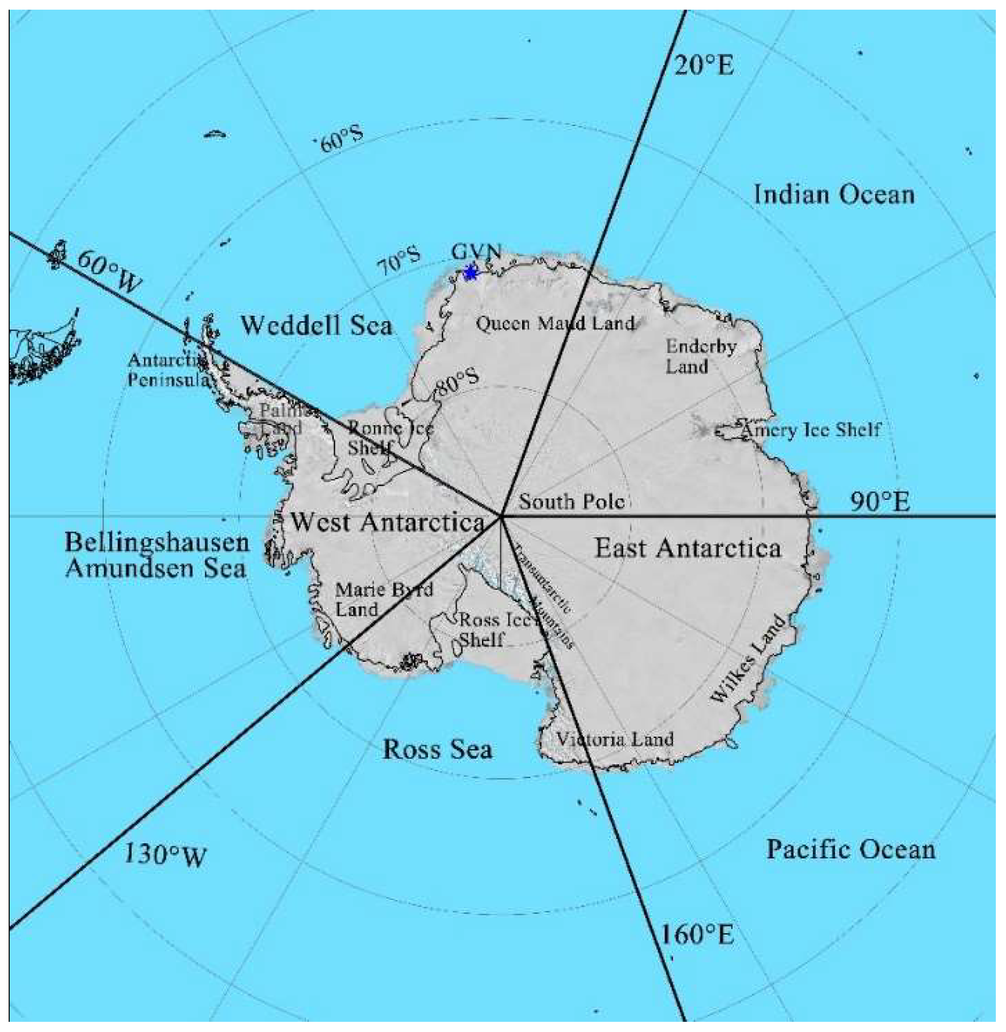
The research region includes the ASIR and five longitudinal sectors ((1). the Weddell Sea (WS), (2). Indian Ocean (IO), (3). Pacific Ocean (PO), (4). Ross Sea (RS), and (5). Bellingshausen–Amundsen Sea (BS)) around Antarctica (Figure 1), from approximately 53°S to 90°S and 180°E to 180°W. The sea surface in the research region varies from open water to a 100% SIC given the research region being on a large scale. The “sea ice region” considered in this study refers to the pixel with a SIC that is greater than 15%, which has been extensively used in other studies [26,38,56]. The monthly SIC products provided by the National Snow and Ice Data Center (NSIDC) are selected as the mask files. If the SIC value of a pixel is greater than 15%, then it will be assigned a value of 1; by contrast, the pixel will be masked. Then, the monthly SAL and SST images are extracted in accordance with the mask file (the mask file is used to multiply the SAL and SST image, month by month). The “sea ice region” varies monthly because the SIC changes dramatically during summer. Thus, using a dynamic mask file to extract the SAL and SST could be justified.
2.2. Datasets
The long-term variations of SAL, SIC and SST were analyzed in this study. The composite albedo of ASIR was provided by the second edition of the satellite–derived climate data record CLARA (“The CM SAF Cloud, Albedo and Surface Radiation dataset from AVHRR data”—second edition denoted as CLARA-A2). The ice concentration data was obtained from SIC products with a spatial resolution of 25 km provided by NSIDC. The National Oceanic and Atmospheric Administration Climate Data Record of the extended APP (APP-x) provided a long-term (1982–present) surface temperature. The ground-site dataset was obtained at the GVN station, which was provided by the Baseline Surface Radiation Network (BSRN).
2.2.1. CLARA-A2
The SAL is provided by the second edition of the satellite-derived climate data record called CLARA-A2 [58,59]. The data record covers a 34-year period from 1982 to 2015. It contains cloud, SAL and surface radiation budget products, which are derived from the AVHRR sensor [60]. The main improvements of CLARA-A2 are cleaning and homogenizing the basic AVHRR level-1 radiance record and systematic use of CALIPSO-CALIOP cloud information for development and validation purposes. The SAL, which is affected by the inherent optical properties of the surface material and atmosphere, depends on atmosphere effects. It is divided into two kinds, namely, black- and white-sky albedos. Black-sky albedo can be defined as the ratio of the radiant flux for light reflected by a unit surface area into the view hemisphere to the illumination radiant flux, when the surface is illuminated with a parallel beam of light from a single direction. Whereas white-sky albedo is the ratio of the radiant flux reflected from a unit surface area into the whole hemisphere to the incident radiant flux of hemispherical angular extent, when the incident radiation is pure diffuse isotropic [61]. The CLARA-A2 SAL terrestrial product is a black-sky albedo (wavelength of 0.25–2.5 µm), which is calculated using cloud mask and AVHRR radiance data. The pentad and monthly mean CLARA-A2 SAL product with a 25 km resolution is used in this study. The CLARA-A2 albedo has been validated against in situ albedo observations from the Baseline Surface Radiation Network, the Greenland Climate Network, and the Tara floating ice camp. Results show a typical accuracy of 3%–15% over snow and ice [62]. The composite albedo (α) of each pixel which comprises open water and sea ice can be defined as:
where Ci and Cw are the area fractions of sea ice and open water, and αi and αw are their albedos, respectively. Due to the narrow range in the albedo of open water, it can be set to a constant value of 7% [63]. The area fractions of sea ice refer to the ice concentration, and only those pixels with an ice concentration greater than 15% are considered in the calculation of sea ice albedo. The pentad mean CLARA-A2 SAL product has been used to estimate the seasonal variation in sea ice albedo. To match the temporal resolution of sea ice albedo, the pentad average of ice concentration is calculated by the average of the daily SIC product.
2.2.2. NSIDC
The Scanning Multichannel Microwave Radiometer on the Nimbus-7 satellite of the National Aeronautics and Space Administration and the Special Sensor Microwave Imager/Sounder sensors on the Defense Meteorological Satellite Program’s -F8, -F11, -F13, and -F17 provide a long-time series of the SIC for investigating the surface characteristics of sea ice covers [11,64,65,66]. The dataset has been generated using the Advanced Microwave Scanning Radiometer-Earth Observing System Bootstrap Algorithm [67]. It is also a key factor in Antarctic climate research and has a significant correlation with the SAL [68]. The monthly SIC data for the South Polar Region are provided by the NSIDC (Bootstrap Sea Ice Concentrations from Nimbus-7 SMMR and DMSP SSM/I-SSMIS, Version 3), with a 25 km spatial resolution. The detailed description of the data and its accuracy can be found in Comiso (2017).
2.2.3. APP-x
The variation in surface temperatures can be used to explain the Antarctic climate change [4,69,70]. The rise in temperature causes snow/ice melt, thereby resulting in an apparent negative correlation between SAL and sea ice surface temperature. The NOAA’s CDR of the extended APP (APP-x) provides a long-time (1982—present) calibrated surface skin temperature data for the Polar Regions [71,72,73]. The APP-x data products are mapped onto a 25-km Equal-Area Scalable Earth-Grid at two local solar times (i.e., 04:00 and 14:00 for the Arctic and 02:00 and 14:00 for the Antarctic). The detailed description and process of the data can be found in the study of Key et al. (2016) [72]. In this study, the surface skin temperature data of the APP-x over the ASIR is used as the SST. The uniformity of illumination is ensured by adopting only the afternoon data (14:00 LT). However, the data for November and December in 1994 and January in 1995 are missing from the archives.
2.2.4. BSRN
The World Climate Research Programme BSRN is established to provide surface radiation measurements of high quality and temporal resolution at a limited number of sites worldwide. Such measurements provide typically 1-min averaged shortwave (SW) surface radiation fluxes. Since the wavelength range of the CLARA-A2 SAL product is between 0.25–2.5 µm, the downwelling and upwelling SW radiation fluxes can be used to estimate the station albedo (αs), as follows:
where ↓ and ↑ represent the downwelling and upwelling SW radiation fluxes, respectively. The GVN station is selected to evaluate the SAL products of CLARA-A2 considering that it is located at the edge of the Antarctic continent. The GVN station (70.65°S, 8.25°W) is located on the Ekstrom Ice Shelf in the northeastern WS. The data is available at the GVN station since 1993. For temporal resolution, the daily and monthly averages are calculated by the average of per minute and day, respectively.
3. Methodology
3.1. EMD
The EMD developed by Huang et al. (1998) was used to analyze the non–linear and non–stationary time series data [47]. The EMD was the base of the Hilbert–Huang transform, which included a Hilbert spectral analysis and an instantaneous frequency computation. After the EMD sifting process, a signal would be decomposed into a finite number of intrinsic mode functions (IMFs) and a residual component, which represents the overall trend of the original signal [44,49,74]. The sifting process was performed as follows:
- (1)
- The local maxima and minima are determined in the original time series data.
- (2)
- A lower/upper envelope (u1(t)/u2(t)) is estimated by fitting cubic splines to the local minima (maxima).
- (3)
- The difference between the original time series data x(t) and the mean of the envelopes m1(t) as the first component h1(t) are defined in accordance with the following equations:
- (4)
- h1(t) is identified as the first IMF c1 if it satisfies the two conditions as follows: (1) throughout the whole length of a single IMF, the numbers of extrema and zero-crossings must either be equal or differ at most by 1; (2) at any data point, the mean value of the envelope defined by the local maxima and the envelope defined by the local minima is 0.
- (5)
- If h1(t) does not satisfy one of these conditions, then it is regarded as a new parameter x(t), and the step in Formulas (1) and (2) is repeated k times until h1k(t) satisfies the conditions or until the difference between the successive sifted results is smaller than the given limit, which is fixed as σthr = 0.3 in our case.
- (6)
- The first IMF is identified as c1 = h1k, and the residual r1(t) can be obtained by subtracting c1 from the original data.
- (7)
- Taking the residual r1(t) as the new data, we repeated Steps 1–6 to determine the next IMF.
- (8)
- The sifting process is stopped until ri(t) becomes a monotonic function or |ri(t)| is very small. Finally, the original signal can be written as follows:
In this study, we defined the residual component rn(t) as the original data trend, which has been extensively used in different fields.
3.2. Slope Test
After the EMD processing, the residual component (trend curve) of the original signal was extracted. It was smoother and more stable than the original signal. The trend curve approximated a straight line over a short time interval. Hence, the first order difference method could be used to study the features of the change trend of the original signal, such as increases in acceleration and deceleration, the transition point of trend curve [75,76]. In this study, the slope test method was used to find the transition point. Its core idea is based on the first order difference method. The method can be expressed as follows:
- (1)
- A subsample s(t) is selected from the original data y(t), and the lengths of the subsample and original data are denoted as j and k, respectively.
- (2)
- The slope of the subsample used in the linear regression equation is calculated aswhere start_time refers to the starting year of the timeseries(l), which corresponds to the subsample; and the function regress is provided by MATLAB R2014b. The function regress is used to estimate the regression coefficients in the linear model at 95% confidence level.
- (3)
- l ∈ (2, j + 1) is set, and Steps 1 and 2 are repeated until l ∈ (k − j + 1, k).
- (4)
- Normally, a slope value that is greater/smaller than 0 indicates an increasing/decreasing trend; in addition, if the sign of the slope transforms from the positive (negative) to the negative (positive) phases, then the trend of the original data has changed and will be defined as the transition point.
The original data are nonlinear and nonstationary; thus, the slope test fails to process these data. The residual component is smoother and more stable than the original data. Thus, the slope test method is adopted to process the residual component to determine the transition point.
4. Validation
The location of the GVN station is shown in Figure 1. Following the evaluation of surface radiation fluxes in Antarctica, the ‘verification area’ refers to the area within 100 km of the GVN station [77,78]. The monthly average of the composite albedo is calculated on the basis of the ‘verification area’ and compared with the data from the GVN site. The statistical parameters contained the mean bias and root mean square error (RMSE).
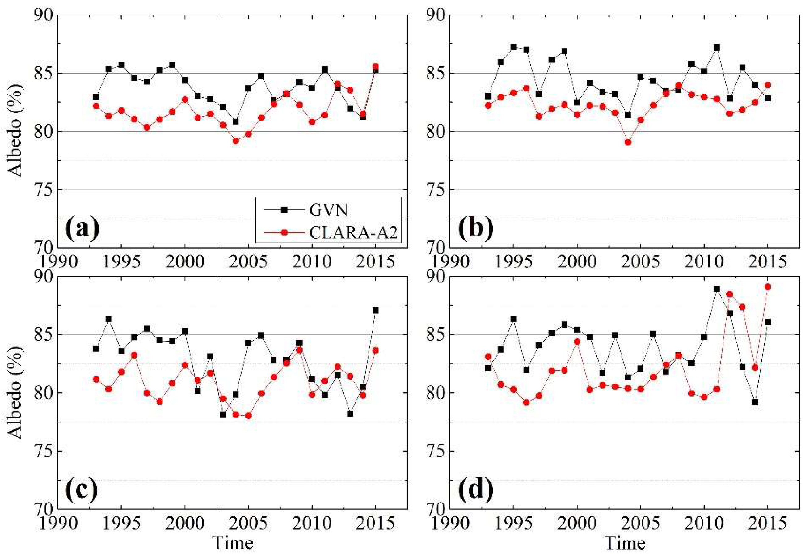
The average albedo derived from the CLARA-A2 SAL product in summer and the months of December, January and February from 1993 to 2015 were validated with those of the GVN station in this study (Figure 2). As shown in the scatter plot (Figure 2a), the albedo estimated from the CLARA-A2 dataset underestimated those in the GVN station during the summer. For each month, the monthly average albedo of CLARA-A2 was also generally lower than those from the GVN site (Figure 2b–d). Hence, the mean biases of summer and each month were less than 0 (Table 2). The mean bias was −2.02% with RMSE of 2.68 during the summer. Moreover, the mean biases and RMSE for each month were greater than −2.5% and lower than 4, respectively. In the light of these results, the accuracy of CLARA-A2 albedo seemed to be consistent with that estimated by Dybbroe et al. (2005) [62].
5. Results and Discussion
5.1. Long-Term Changes and Trends
The variability and trends of the SAL, SIC and SST were presented in the form of a time series of summer averages for 1982–2015. The time series were calculated for the ASIR as a whole and for the five longitudinal sectors. The SAL, SIC and SST for these sectors were calculated by time- and area-averaging all the values from pixels identified as sea ice for each region. The residual component could present the trend of the original signal; thus, it was used to estimate the slope values. To determine the optimal linear fit for the residual component, the slope values were estimated through the least squares method. The statistical significance of each slope value is tested using a standard F-test with a confidence of 95% and 99%. The yearly relationship between these variations is illustrated in Figure 3, Figure 4 and Figure 5.
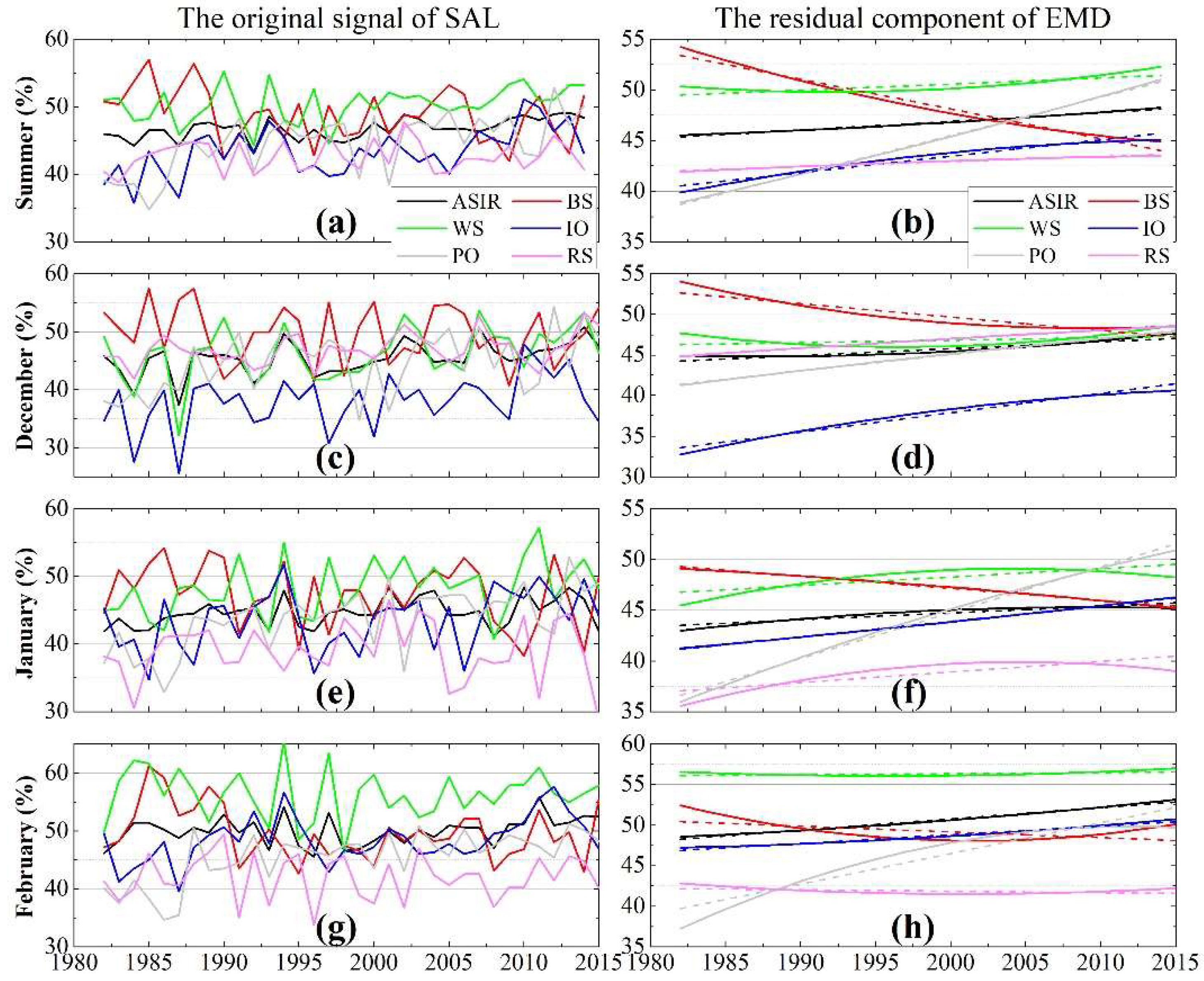
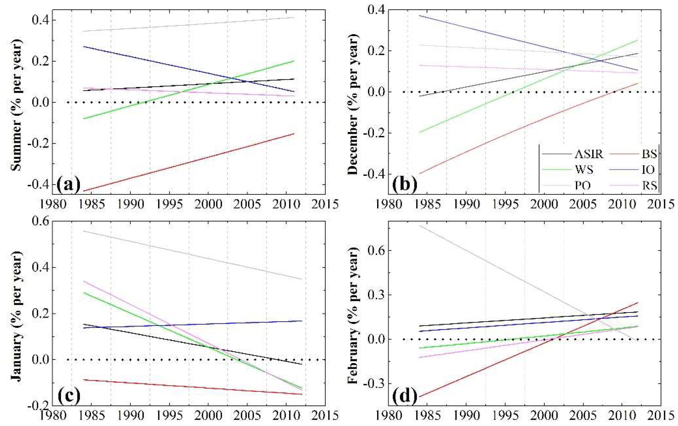
The trend of SAL for the ASIR and the five longitudinal sectors exhibited various degrees of the increasing trend throughout the time series during summer, except for the BS, which showed a significant decreasing trend (Figure 3). This was generally contrary to that in the Arctic [56]. Furthermore, the trend of the BS also showed negative for each month (Figure 3d,f,h), thereby indicating that the climate in the BS presents a warming trend during summer [13,79]. In December, the lowest values of SAL were found in the IO, except for after 2010 (Figure 3c). This was consistent with the results by Shao et al. (2015) [39]. The SAL in the WS and the RS clearly increased before 2002 and slightly decreased after 2002 (Figure 3f), which may have been caused by a negative sea level pressure which occurred in the early 2000s [80]. However, that in BS showed a decreasing and increasing trend before and after 2000, correspondingly (Figure 3h). This finding suggested that further analysis of the trend of SAL is required.
The slope values of SAL in the BS were negative during summer and for the 3 months (Table 3) due to an anticyclonic circulation trend and equatorward winds in the Bellingshausen Sea enhanced the heat exchange with lower latitudes [7]. However, those in the ASIR and other sectors were positive, except for those in the RS during February. These results demonstrated that the climate of the ASIR exhibits a cooling trend during summer [24], except for the BS [81]. The trend of the SAL in the RS during December and January could dominate that of February, thereby causing a positive slope value during summer. The steepest positive trend was identified in the PO during summer (3.781% per decade), largely caused by the trade winds in the Pacific, have significantly strengthened during the past two decades [82]. This result was consistent with the results of Laine (2007) [38]. The maximum averages of the SAL existed in the WS (50.38%) during summer, which could be partly explained by the fact that maximum sea ice extents existed in WS [21].
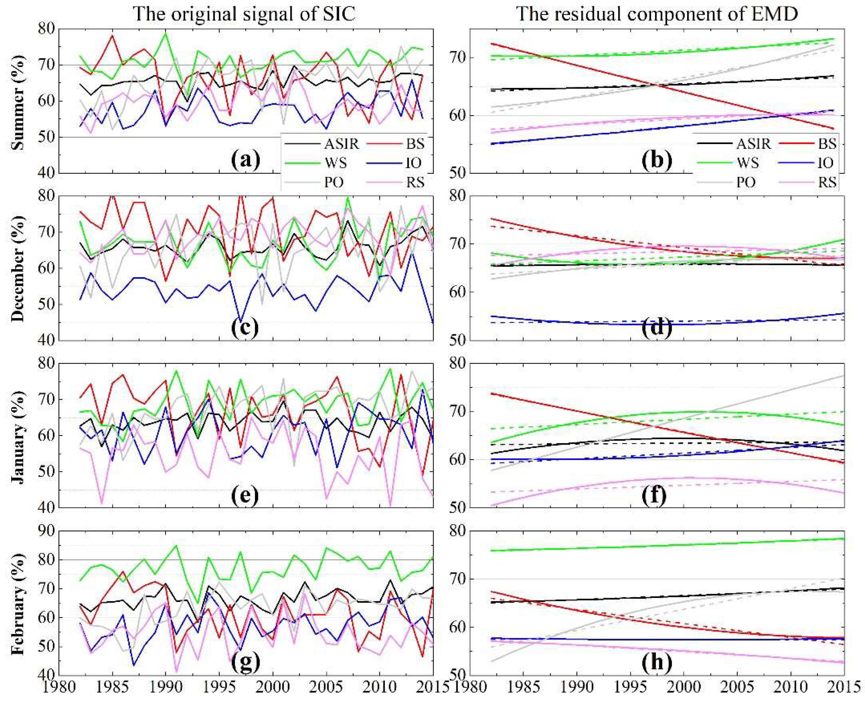
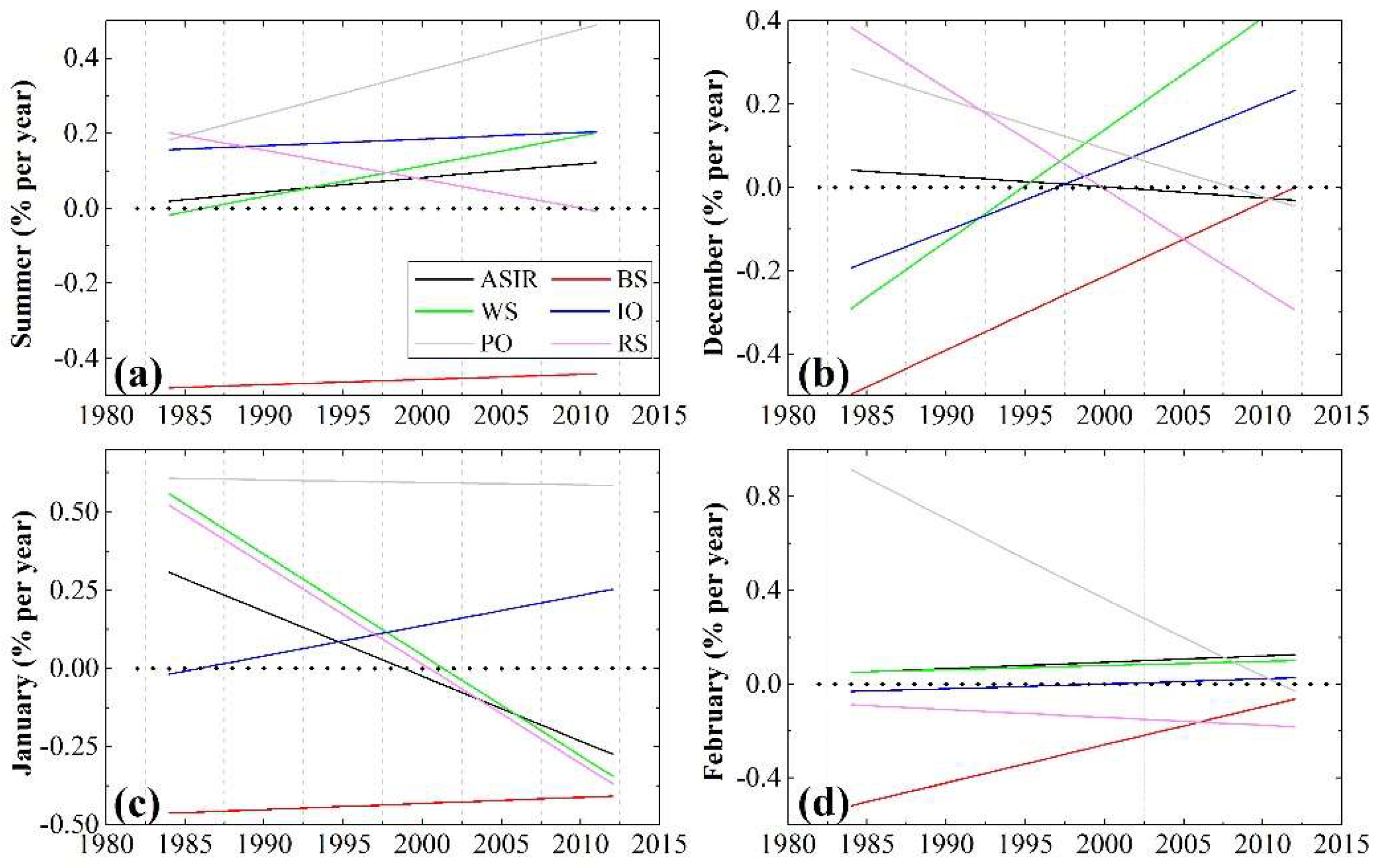
Similar to the trend of the SAL, that of the SIC showed an evidently increasing trend during the summer, except for the BS (Figure 4b), as estimated by Holland (2014) and Hobbs et al. (2016) [55,83], thus illustrating a significant positive correlation between the SAL and the SIC. This can be explained by the slowdown of the global warming trend and a deepening of the Amundsen Sea Low near Antarctica [25,84]. In contrast to the change of SIC in the BS, that in the PO presented an increasing trend (Figure 4d,f,h), and the fastest increasing trend was observed in January when the Southern Annular Mode had positive results in more and stronger cyclones [85]. Interestingly, the decreasing/increasing trend of the SIC in the BS/PO became relatively flat after 2000 (Figure 4h), this may be caused by the fact that the temperature has remained flat for the past 15 years [84]. However, the trend of the SIC showed a crest/trough for the RS/IO around 2000 (increasing/decreasing before 2000 and decreasing/increasing after 2000) (Figure 4d). This finding indicated that a transition point of climate change may have existed in the RS/IO around the year 2000.
Consistent with the trend of SAL, the slope values of SIC were mostly positive, except for the BS (Table 4) [25], which further demonstrated that the climate of the ASIR exhibits a cooling trend in recent decades. The steepest increasing trend could be observed in the PO during the summer and each month [7], and the largest slope values were determined in January (5.968% per decade). Clearly, the increasing rate of sea ice was slower in West Antarctica (WS, BS, and RS) than in East Antarctica (IO and PO), which is consistent with the changes in the surface net radiation reported by Zhang et al. (2019) [78]. This result was due to the more severe climate change in West Antarctica than in East Antarctica [4,86]. The average of the SIC in the WS was highest during the summer and the 3 months considering substantial multiyear sea ice [87]; however, simultaneously, that in the IO was the lowest largely because of substantial solar radiation absorbed by the East Antarctica sea ice due to the low solar zenith angle [88,89].
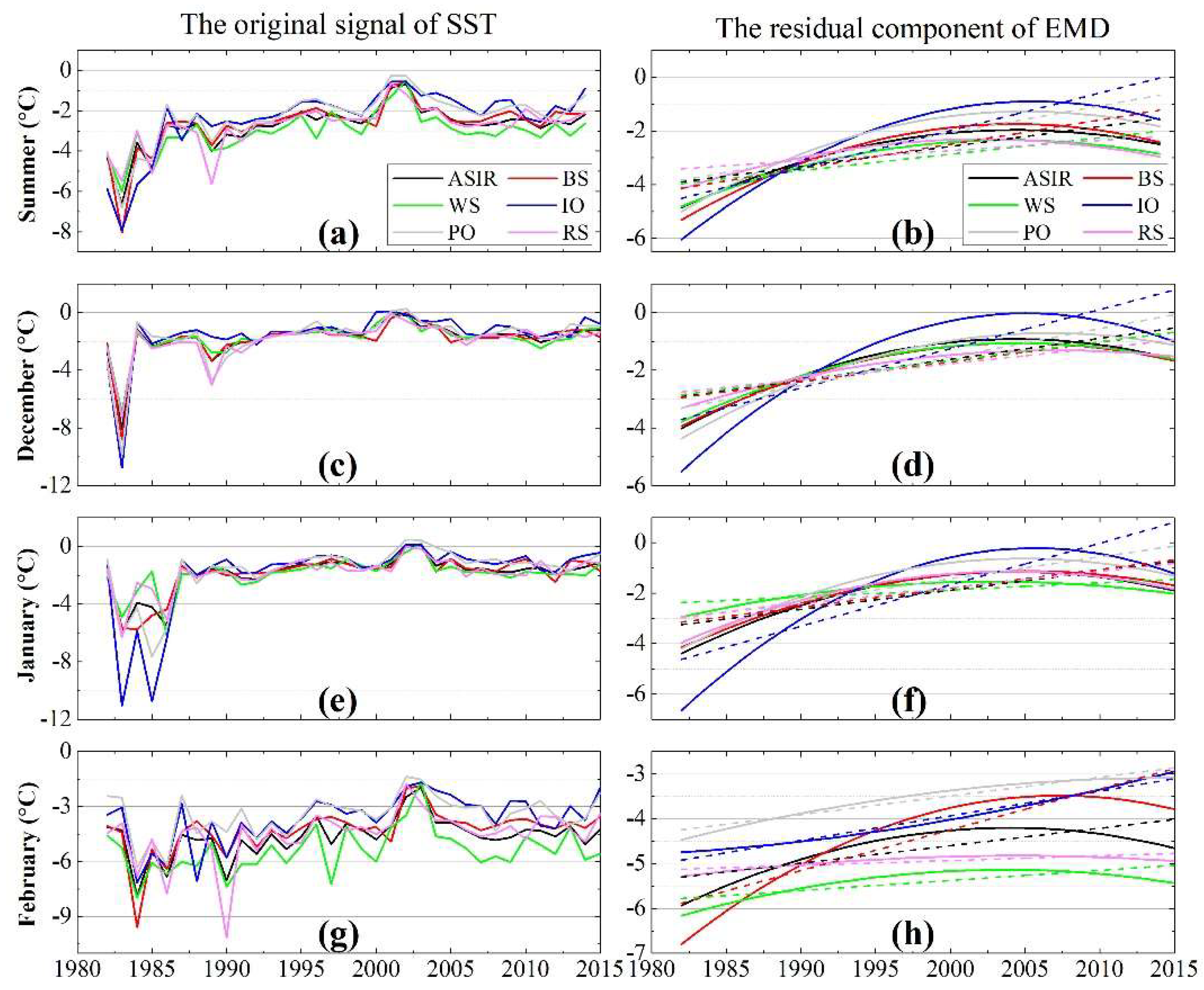
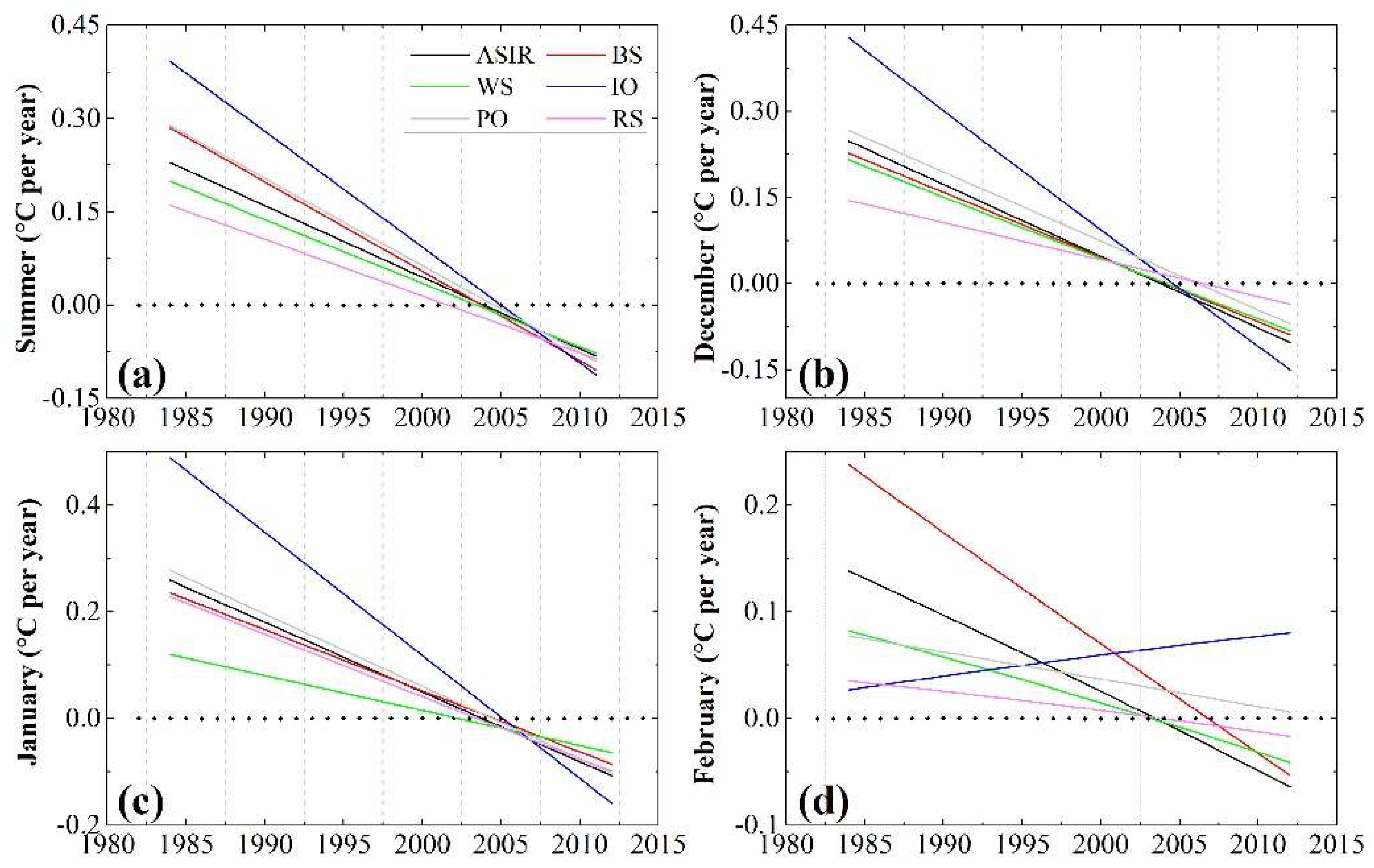
The change in SST in the ASIR and the five longitudinal sectors presented a significant increasing trend during the summer and the 3 months (Figure 5). This change was largely caused by the low SST values before 1988. Notably, the time series curves of the SST in the ASIR and the five longitudinal sectors had considerable peak values near 2002/2003 (Figure 5a,c,e,g); moreover, a crest appeared between 2000 and 2005 for the trend curves of the SST (Figure 5b,d,f,h); this may be caused by the Interdecadal Pacific Oscillation which transitioned from positive to negative in the late 1990s [7]. This result indicated that a climate transition point exists around the year 2000; this change was similar to that of SAL/SIC. Although the solar zenith angles were lowest in the ASIR during summer [27,90], its SST was below 0 °C.
The low SST values in the ASIR and the five longitudinal sectors before 1988 would dominate given the evident increasing trend of temperature, and it seems to be a noisy signal due to the AVHRR-7/9 which had some serious calibration issues; therefore, the slope values (°C per decade) and the average of the SST during the summer and the 3 months for the ASIR and the five longitudinal sectors in 1988–2015 were calculated (Table 5). The trends of SST were nearly positive (with a 99% confidence level) despite the low values of temperature before 1988 were removed; these were similar to the results indicated by Shu et al. (2012) [49]. This result illustrated that the long-term slope values of temperature may conceal the short-term features of climate change. The slope values of the SST were greater in East Antarctica than in West Antarctica during summer and the 3 months because East Antarctica was basically under an ice-free state during the summer [66]. Thus, the average of the SST was also higher in East Antarctica than in West Antarctica [39]. The average of the SST for February was the lowest in the 3 months due to the fact that the end of summer is February in Antarctica.
5.2. Seasonal Evolution of Composite Albedo, SIC and Sea Ice Albedo
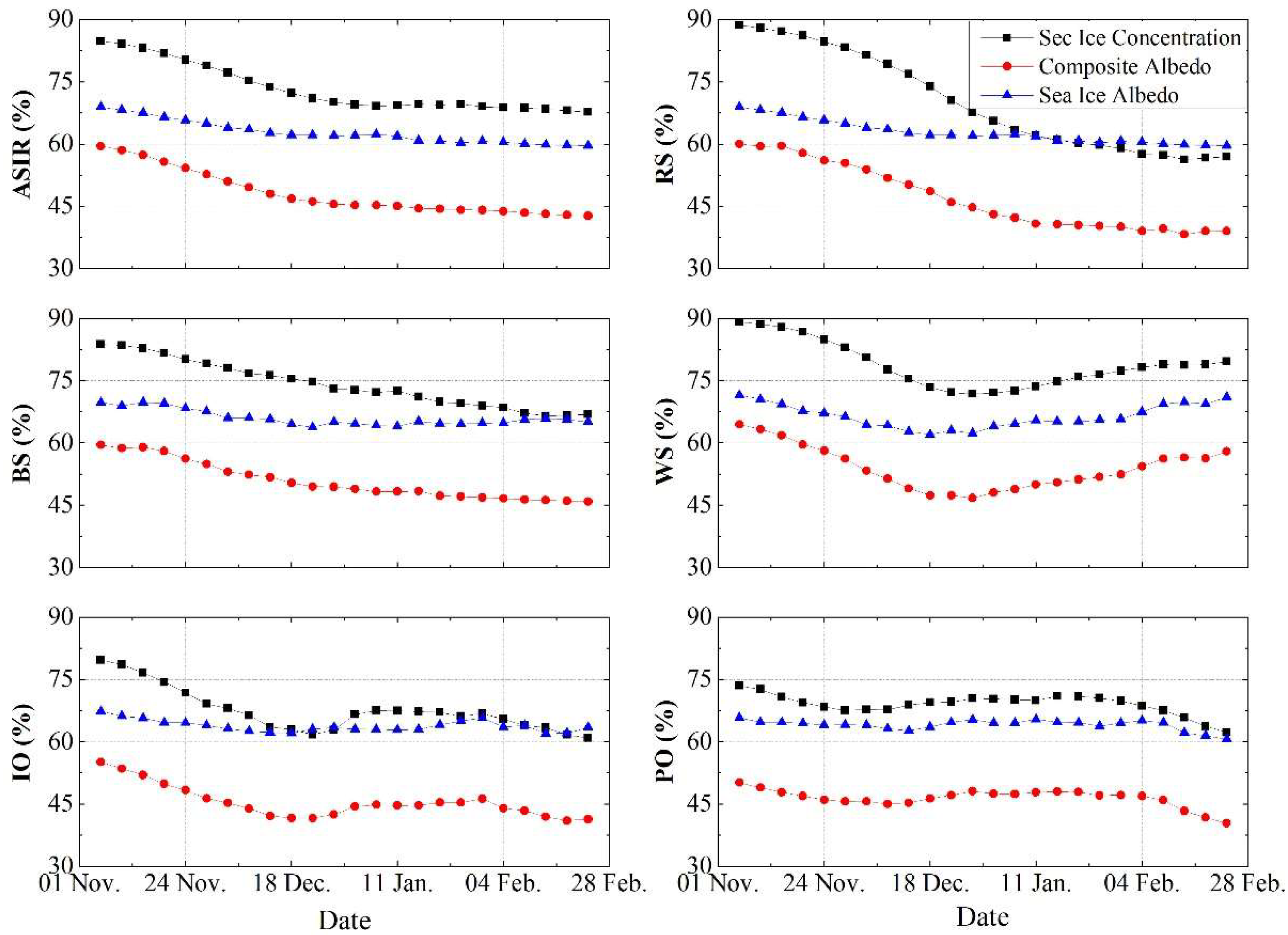
To study the changes in composite albedo, SIC and sea ice albedo during summer, their seasonal evolution were presented in the form of 5-day averages from 1 November to 28 February over 1982–2015 (Figure 6). Table 6 presents the relationships of composite albedo and SIC or sea ice albedo. For the ASIR, the changes in composite albedo, SIC and sea ice albedo showed a decreasing trend throughout the time series during summer, and the relationship between composite albedo and SIC (0.992, above 99% confidence level) or sea ice albedo (0.980, above 99% confidence level) exhibited a strong correlation. This finding could be explained by the substantial incident solar irradiance absorbed by the ice-ocean system due to the low solar zenith angles during summer [78]. The decreasing process during the entire summer could be divided into two phases. The first phase lasted until late December, wherein the composite albedo and SIC presented a rapidly decreasing trend, from 60% and 85% to 45% and 70% for composite albedo and SIC, respectively. However, that of sea ice albedo was distinctly slow, from 70% to 60%, which may be caused by the convergent winds in early summer, thereby driving the ice edge retreat poleward and activating the ice-albedo feedback [91]. The decreasing trend was relatively slow after late December, largely due to the negative sea level pressure anomalies that occurred around Antarctica during late summer [55]. Therefore, the evolution of composite albedo, SIC and sea ice albedo depended mainly on the early melting of sea ice during summer.
The evolution of composite albedo closely followed the change in SIC (with a strong correlation coefficient (0.99) at 99% confidence level). Thus, a rapid decrease in composite albedo was observed before mid-January over RS (from 60% to 37%), and a stable level (35%) was maintained subsequently. These findings could be partly explained by the presence of deep cyclones, which would efficiently break up and export the sea ice equatorward [85]. However, after a slightly decease before mid-December, the sea ice albedo maintained a relatively stable level (60%) and reached a stable level earlier, at approximately one month before composite albedo, which was similar to that in the Arctic reported by Lei et al. (2016). Consistent with other studies [14,21,92], the composite albedo and SIC in BS presented a steady decreasing trend during the entire summer. However, the decreasing trend of sea ice albedo was evidently slower than that of composite albedo and SIC. Interestingly, the time series plots of composite albedo, SIC and sea ice albedo showed a significant trough by the end of December in WS. This phenomenon may be due to the predominantly westerly wind trends over most of the Southern Ocean during summer and enhanced equatorward winds that existed in mid-summer over WS, thereby increasing the sea ice [80].
The sea ice extent in East Antarctica was relatively lower than that in West Antarctica and was accompanied by complex change in wind field and dramatic melt during summer [16,93]. The changes in sea ice in the IO and PO did not show a monotonic downward trend. After a rapid decline before mid-December, the sea ice in the IO maintained a short increasing process (approximately half a month). From then onward, a gradually decreasing trend was observed. The evolution characteristics of sea ice in the PO were similar to those in the IO, but had a slow change trend and long rising process (approximately one and a half months). This phenomenon was mainly caused by the change in sea-level pressure in East Antarctica which was stable and the enhanced westerly winds that would transport sea ice from the IO to the PO during summer [7]. The relationships between composite albedo and SIC were 0.975 and 0.957 in the IO and PO (with a 99% confidence level), respectively. However, the correlation between composite albedo and sea ice albedo were both below 0.9 (with a 99% confidence level) in the two regions, indicating that the evolution of composite albedo during summer depends more strongly on the change in SIC than on the variation in sea ice albedo.
5.3. Transition Points of the SAL, SIC, and SST
According to the abovementioned time series and trend analysis, a climate transition point existed in the entire ASIR around 2000–2005. Moreover, for the SAL, SIC and SST, the slope values of the long_time series would obscure the short-term characteristics of climate change. Therefore, the slope test method was used to estimate the residual components of the SAL, SIC and SST to determine the transition point. The time series curves of the residual component were smooth; thus, the length of the subsample was defined as 5 years. If the slope line had passed through the zero line, then a transition point would exist at that moment. For a detailed analysis of the SAL, SIC and SST variation trends during summer and the 3 months for the ASIR and the five longitudinal sectors, we performed a morphological analysis of the residual component and found that morphological variations can be broadly divided into four categories, namely, increasing, increasing–decreasing, decreasing–increasing, and decreasing types.
The time series of the slope values of the SAL during summer and the 3 months are plotted in Figure 7. The transition point of the SAL only existed in the WS during summer, and the increasing/decreasing trend of the SAL exhibited deceleration in the IO/BS (Figure 7a), similar to those observed in the Antarctic ice sheet [41]. The SAL of the ASIR presented a slightly upward trend despite the fact that in the BS decreased rapidly, this was opposite to that in the Arctic sea ice zone [56]. For each month, the slope lines of the IO and the PO were constantly greater than the zero line (Figure 7b–d), which were located in East Antarctica. The change trend types and transition point of the SAL are presented in Table 7. The decreasing–increasing type existed in December and February, and the increasing–decreasing type appeared in January. The transition point in West Antarctica occurred in February 2000 which is consistent with the climate change on the Antarctic Peninsula [94].
Although the slope values of the SIC were approximately greater than 0, except for the BS during summer (Figure 8a) [24], the time series of the slope lines for different regions showed different features. For example, the increasing trend in the PO and the RS exhibited acceleration and deceleration, correspondingly [21,24,95], whereas the slope values of the SIC in the IO were essentially constant. The slope lines of the PO and the BS were above and below the zero line during the 3 months (Figure 8b–d), respectively; these slope lines were similar to the SAL. However, the features of the slope lines for the different months were complex and changeable over other regions. This result was largely due to the dramatic climate change during the ASIR summer [13,44]. The transition points of the SIC in the ASIR appeared in December 2001 and January 1999 because that in the five longitudinal sectors appeared around the year 2000, except for the BS and PO (Table 8).
The slope lines of the SST for the ASIR and the five longitudinal sectors were positive before 2000–2005 and negative afterward (Figure 9a). This result demonstrated that a cooling trend of climate occurs in the whole ASIR in 2000–2005 [80]. During summer, the slowest increasing trend of the SST appeared in the PO before 2000 [96,97]. Although the slope lines were above the zero line in February (Figure 9d), the warming trend in the IO and the PO presented acceleration and deceleration, respectively. In contrast to the characteristics of the slope lines of SAL/SIC, the morphological type of the SST in the ASIR and the five longitudinal sectors during summer and the 3 months was increasing–decreasing, except for that in the PO and IO in February (Table 9). Furthermore, the transition points of the ASIR and the five longitudinal sectors were around 2003–2005 and are generally in step with global surface temperature change [98].
5.4. Spatial Distribution
To illustrate the average spatial distributions of the SAL, SIC and SST, the maps were prepared for the average summer SAL, SIC and SST of the whole ASIR for the entire 33 years (Figure 10).
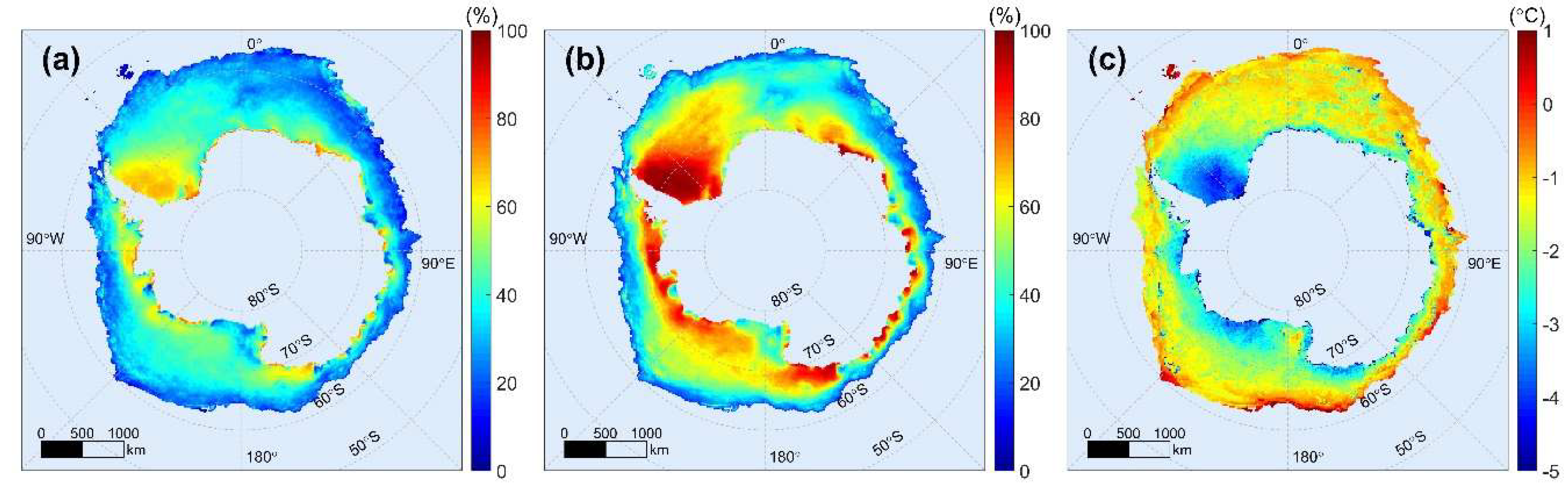
Because positive sea-level pressure anomalies and northward winds appeared in the Southern Atlantic Ocean [7], the SIC in the WS was high during summer (Figure 10b); thus, the high SAL could also be found in the WS (Figure 10a) [37,83]. Moreover, the low values of the SST existed in the WS (Figure 10c), thereby indicating that the spatial correlation between the SAL and the SIC was significantly positive, and that between SAL/SIC and SST was negative [99]. The low pixel average of SAL/SIC and high pixel average of the SST appeared on the edge of the sea ice, which was largely due to the solar radiation that was absorbed when the latitude was low [31], and positive (negative) cyclone density anomalies emerged around Antarctica (mid-latitudes) [85]. Minimal sea ice existed in East Antarctica; thus, the SAL and SIC were evidently smaller in East Antarctica than in West Antarctica. The average SAL (Table 3), SIC (Table 4), and SST (Table 5) for the total ASIR were 46.75%, 65.39%, and −2.44 °C during summer.
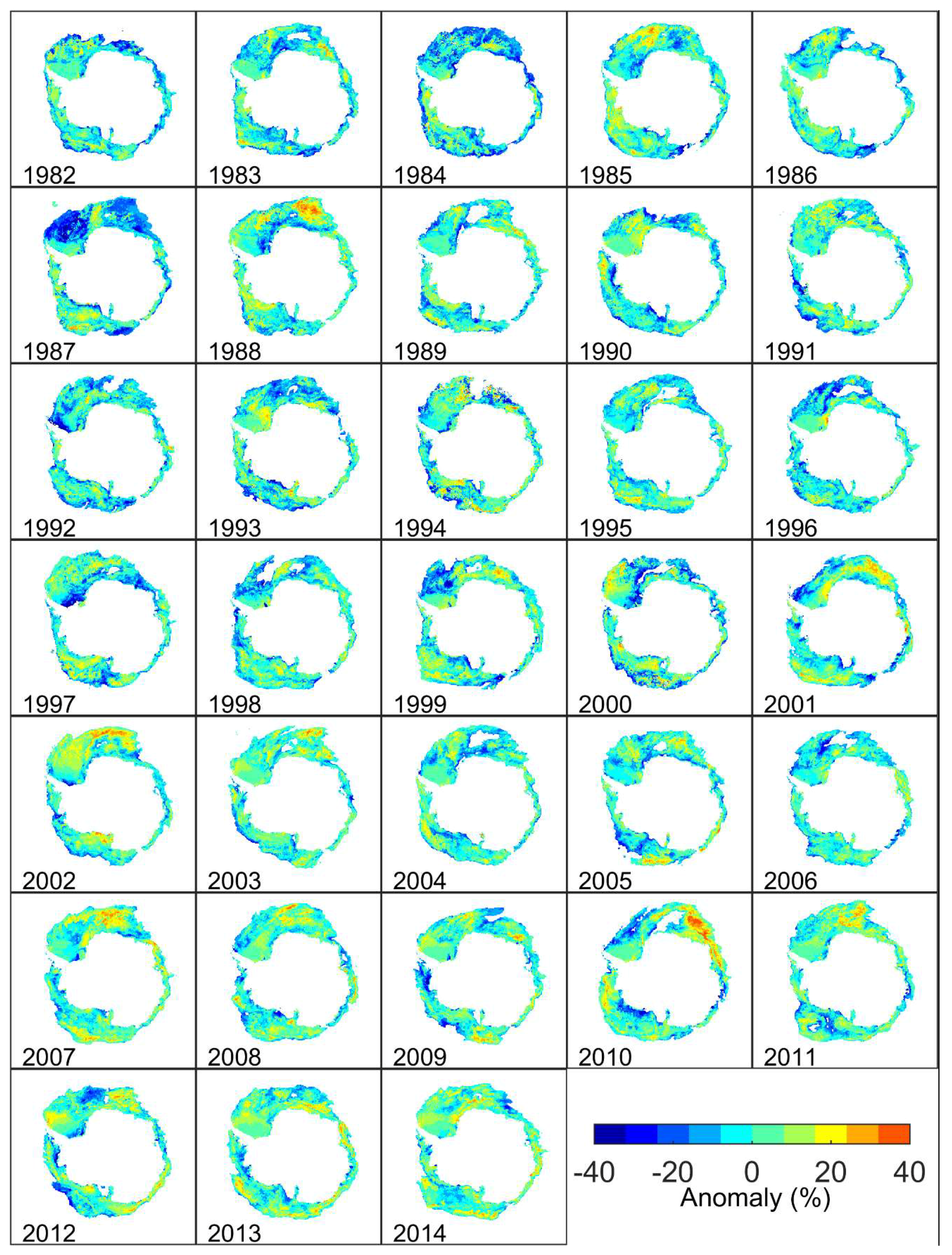
For further analysis of the sea ice albedo variations from 1982 to 2014 during the summer, the anomaly maps of the summer SAL could provide an illustrative way of estimating the overall changes from year to year (Figure 11). These maps were generated by taking the difference between the summer SAL for each year and the corresponding average for the entire 33 years [12]. In Figure 11, the SAL varied significantly from year to year during the study period. The anomaly values in several areas of the WS were negative before 2001, and they turned into positive after 2001, thereby demonstrating that the SAL of these areas in the WS has a transition point around 2001, which was highly consistent with the climate change in the Antarctic Peninsula during recent decades [5,94]. Moreover, for the whole ASIR, the anomaly values of the SAL were clearly higher after 2001 than before 2001. Relatively strong negative SAL anomalies for the WS and Haakon VII Sea occurred in 1984 and 1987.
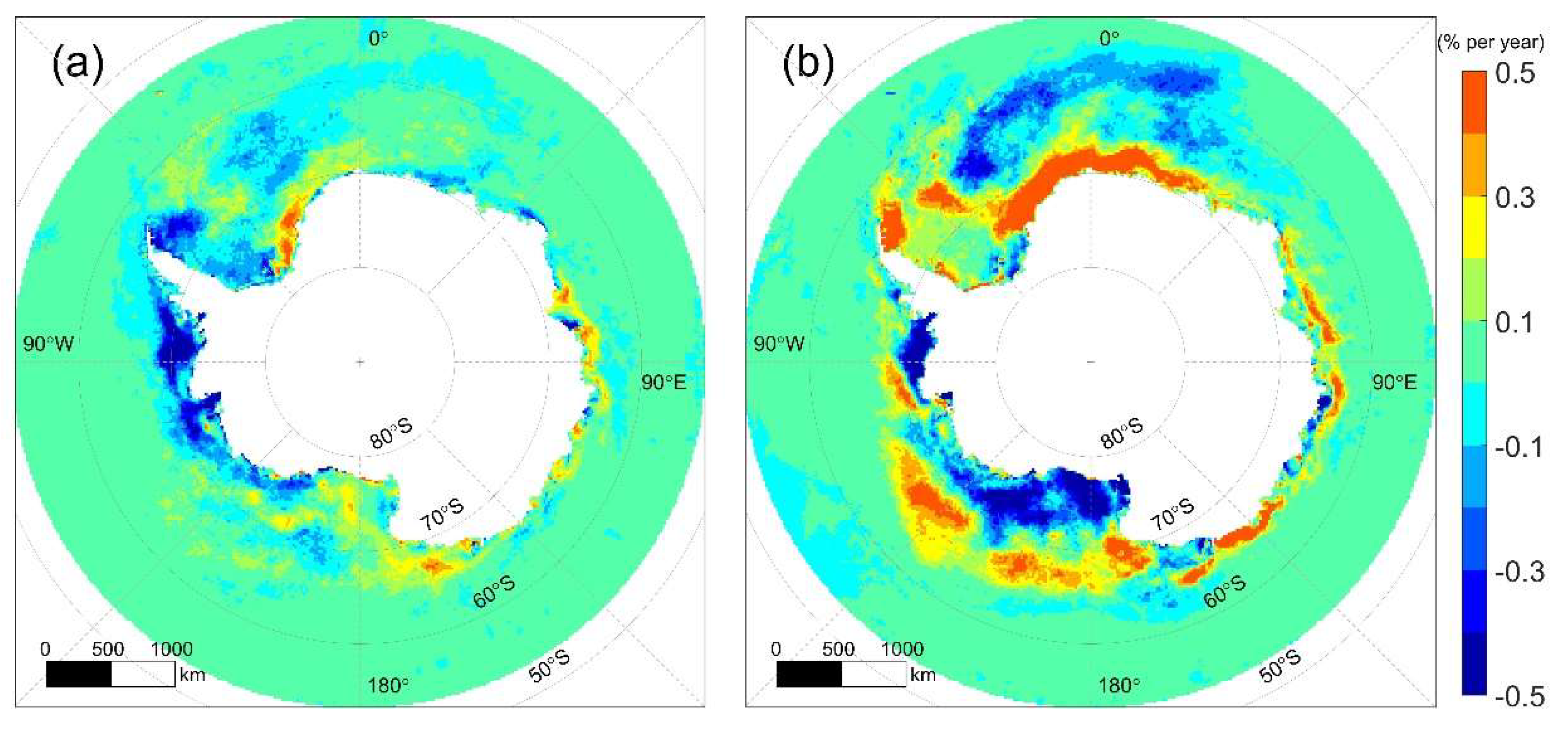
The abovementioned research indicated that the climate in the whole ASIR may have warmed before 2001 and changed to cooling after 2001. Thus, we selected 2001 as the transition point to calculate the pixel-based spatial trend distribution maps of the SAL (Figure 12). The trends were calculated pixel-by-pixel through the least squares method for determining the best linear fit for the data. The trends were positive for most of East Antarctica before 2001 (Figure 12a). A deeply negative trend was observed along the coast of Ellsworth Land and east of the Antarctic Peninsula due to a negative phase of sea-level pressure and a poleward wind would strengthen heat exchange [16]; this result is consistent with the results of Shao et al. (2015) [39]. The strongly positive trend of the SAL was found only on the coast of Coats Land before 2001. Although the trend of the SAL in many areas of West Antarctica increased after 2001, the increasing speed was lower in West Antarctica than in East Antarctica (Figure 12b) and was mainly caused by the deeply negative trend that existed in the RS and the BS [38]. However, the trend of the SAL in most areas of West Antarctica after 2001 was opposite to that before 2001, especially in the east of the Antarctic Peninsula; this finding is similar to that of Oliva et al. (2017) [94]. The SAL in the coast of the Dronning Maud Land exhibited a strongly positive trend; however, the SAL in low latitudes (57°S–67°S,30°E–40°W) showed a significant negative trend (Figure 12b). This could result in stable SAL for the entire WS throughout the time series.
6. Conclusions
In this study, the climate change of the entire ASIR has been studied in recent decades by analyzing the long-term changes in SAL, SIC and SST. The EMD method was used to extract the trend of the original signal, and the slope-test method was applied to determine the transition points of SAL, SIC and SST. The SAL derived from the CLARA-A2 product was compared with measurements obtained at the GVN station. The analysis showed that the transition point of climate for the entire ASIR can be observed around 2000–2005. A further study of the spatial distribution of the SAL demonstrated that the transition point is around 2001. The detailed analysis results are presented as follows:
The trend of the SAL and SIC for the ASIR and the five longitudinal sectors exhibited a positive trend throughout the time series, except for the BS, which showed a significant negative trend (−2.926% and −4.596% per decade for the SAL and SIC, correspondingly) during the summer. Moreover, the steepest increasing trend of the SAL and SIC occurred in the PO, with approximately 3.781% and 3.358% per decade (at a 99% confidence level). The average of the SAL and SIC (50.38% and 70.99%, respectively) were higher in the WS than in other sectors during summer. In contrast to the changes in SAL/SIC, the trend curves of the SST for the ASIR and the five longitudinal sectors peaked around 2000–2005 during summer and the 3 months, and the maximum average of the SST occurred in 2002/2003. The trends of the SST presented a positive trend (basically with a 99% confidence level).
The seasonal evolution of composite albedo, SIC and sea ice albedo for the ASIR illustrated that their changes had a rapidly decreasing trend during early summer, and then maintained a relatively stable level or decreased gradually. Moreover, the relationship between composite albedo and SIC or sea ice albedo exhibited a significant correlation coefficient, at approximately 0.992 or 0.98 (at 99% confidence level), respectively. The change in summer albedo depends mainly on the early melt of sea ice during summer. For the five longitudinal sectors, the change trend of sea ice albedo was slower and reached a stable level earlier than those of composite albedo and SIC. The correlations between composite albedo and SIC or sea ice albedo were basically higher than 0.9 or 0.7 (with a 99% confidence level), respectively.
The slope lines of SAL/SIC for the ASIR and the five longitudinal sectors were nearly above the zero line during summer, except for the BS. Evidently, the increasing trend of SAL/SIC in the PO accelerated, and the decreasing trend of them in the BS slowed down. Although the slope lines of SAL/SIC were changing for the 3 months, their transition point was around 2000. The change trend types of the SST for the ASIR and the five longitudinal sectors mostly presented an increasing–decreasing trend during summer and the 3 months. Furthermore, the transition points of the SST were around 2003–2005.
For the spatial distribution of pixel average, the high values of SAL and SIC appeared in the WS during summer; and the low values of the SST could also be observed there in the meantime. Furthermore, the pixel average of SAL/SIC decreased with latitude, but this result was contrary to that of the SST. The anomaly maps of the SAL illustrated that the transition point has occurred around 2001 in West Antarctica, especially in the WS. Then, 2001 was selected as the transition point for calculating the pixel-based trend of the SAL. We found that the climate of West Antarctica has transformed from warming before 2001 to cooling after 2001 for most areas, except for the BS. This phenomenon was particularly significant in the east of the Antarctic Peninsula. However, the climate of East Antarctica had shown a cooling trend in recent decades.
A long-term analysis of several factors will mask short-term features of climate change, and removing some point or changing the starting or ending times of the linear regression analysis can alter the linear trend or the value of slopes. In addition, the change in summer sea ice albedo also depends strongly on the ice surface melting and melt ponds. In the future, the characteristics of climate change for regional areas of Antarctica will be further analyzed. Moreover, an analysis of other factors, such as sea ice thickness, solar radiation, melt pond fraction, and cloud cover, will be carried out.
Author Contributions
C.Z. and T.Z. contributed the main idea and designed the research; C.Z., T.Z. and L.Z. performed the experiments and analyzed the data; C.Z. and T.Z. wrote the manuscript; and all authors contributed to and approved the final manuscript.
Funding
This research was supported by the National Natural Science Foundation of China (No. 41376187, 41531069 and 41776200) and the National Key Research and Development Program of China (2018YFC1406100).
Acknowledgments
We sincerely want to thank the EUMETSAT Climate Monitoring Satellite Application Facility (CM SAF) project to provide the CLARA-A2-SAL dataset. We are very grateful for the sea ice concentration data provided by the National Snow and Ice Data Center. We are also thankful the National Oceanic and Atmospheric Administration (NOAA) Climate Data Record (CDR) provided with the APP-x dataset.
Conflicts of Interest
The authors declare no conflict of interest.
References
- Bracegirdle, T.J.; Connolley, W.M.; Turner, J. Antarctic climate change over the twenty first century. J. Geophys. Res. Atmos. 2008, 113. [Google Scholar] [CrossRef] [Green Version]
- Alley, K.E.; Scambos, T.A.; Siegfried, M.R.; Fricker, H.A. Impacts of warm water on Antarctic ice shelf stability through basal channel formation. Nat. Geosci. 2016, 9, 290. [Google Scholar] [CrossRef]
- Hobbs, W.R.; Bindoff, N.L.; Raphael, M.N. New perspectives on observed and simulated Antarctic sea ice extent trends using optimal fingerprinting techniques. J. Clim. 2015, 28, 1543–1560. [Google Scholar] [CrossRef]
- Turner, J.; Colwell, S.R.; Marshall, G.J.; Lachlan-Cope, T.A.; Carleton, A.M.; Jones, P.D.; Lagun, V.; Reid, P.A.; Iagovkina, S. Antarctic climate change during the last 50 years. Int. J. Climatol. 2005, 25, 279–294. [Google Scholar] [CrossRef] [Green Version]
- Turner, J.; Lu, H.; White, I.; King, J.C.; Phillips, T.; Hosking, J.S.; Bracegirdle, T.J.; Marshall, G.J.; Mulvaney, R.; Deb, P. Absence of 21st century warming on Antarctic peninsula consistent with natural variability. Nature 2016, 535, 411–415. [Google Scholar] [CrossRef] [PubMed]
- Steig, E.J. Climate science cooling in the Antarctic. Nature 2016, 535, 358–359. [Google Scholar] [CrossRef] [PubMed]
- Meehl, G.A.; Arblaster, J.M.; Bitz, C.M.; Chung, C.T.Y.; Teng, H. Antarctic sea-ice expansion between 2000 and 2014 driven by tropical pacific decadal climate variability. Nat. Geosci. 2016, 9, 590–595. [Google Scholar] [CrossRef]
- Schemm, S. Regional trends in weather systems help explain Antarctic sea ice trends. Geophys. Res. Lett. 2018, 45, 7165–7175. [Google Scholar] [CrossRef]
- Jena, B.; Kumar, A.; Ravichandran, M.; Kern, S. Mechanism of sea-ice expansion in the Indian ocean sector of Antarctica: Insights from satellite observation and model reanalysis. PLoS ONE 2018, 13, e0203222. [Google Scholar] [CrossRef] [PubMed]
- Hanna, E. The role of Antarctic sea ice in global climate change. Prog. Phys. Geogr. 1996, 20, 371–401. [Google Scholar] [Green Version]
- Zwally, H.J.; Comiso, J.C.; Parkinson, C.L.; Cavalieri, D.J.; Gloersen, P. Variability of Antarctic sea ice 1979–1998. J. Geophys. Res. Ocean. 2002, 107, 9-1–9-19. [Google Scholar] [CrossRef]
- Ferreira, D.; Marshall, J.; Bitz, C.M.; Solomon, S.; Plumb, A. Antarctic ocean and sea ice response to ozone depletion: A two-time-scale problem. J. Clim. 2015, 28, 1206–1226. [Google Scholar] [CrossRef]
- Jones, J.M.; Gille, S.T.; Goosse, H.; Abram, N.J.; Canziani, P.O.; Charman, D.J.; Clem, K.R.; Crosta, X.; de Lavergne, C.; Eisenman, I.; et al. Assessing recent trends in high-latitude southern hemisphere surface climate. Nat. Clim. Chang. 2016, 6, 917–926. [Google Scholar] [CrossRef]
- Turner, J.; Hosking, J.S.; Bracegirdle, T.J.; Marshall, G.J.; Phillips, T. Recent changes in Antarctic sea ice. Philos. Trans. R. Soc. A Math. Phys. Eng. Sci. 2015, 373. [Google Scholar] [CrossRef] [PubMed]
- Turner, J.; Orr, A.; Gudmundsson, G.H.; Jenkins, A.; Bingham, R.G.; Hillenbrand, C.-D.; Bracegirdle, T.J. Atmosphere-ocean-ice interactions in the Amundsen Sea embayment, West Antarctica. Rev. Geophys. 2017, 55, 235–276. [Google Scholar] [CrossRef]
- Turner, J.; Phillips, T.; Marshall, G.J.; Hosking, J.S.; Pope, J.O.; Bracegirdle, T.J.; Deb, P. Unprecedented springtime retreat of Antarctic sea ice in 2016. Geophys. Res. Lett. 2017, 44, 6868–6875. [Google Scholar] [CrossRef] [Green Version]
- Kusahara, K.; Reid, P.; Williams, G.D.; Massom, R.; Hasumi, H. An ocean-sea ice model study of the unprecedented Antarctic sea ice minimum in 2016. Environ. Res. Lett. 2018, 13, 084020. [Google Scholar] [CrossRef]
- Curry, J.A.; Schramm, J.L.; Ebert, E.E. Sea-ice albedo climate feedback mechanism. J. Clim. 1995, 8, 240–247. [Google Scholar] [CrossRef]
- Hall, A. The role of surface albedo feedback in climate. J. Clim. 2004, 17, 1550–1568. [Google Scholar] [CrossRef]
- Katlein, C.; Hendricks, S.; Key, J. Brief communication: Increasing shortwave absorption over the Arctic ocean is not balanced by trends in the Antarctic. Cryosphere 2017, 11, 2111–2116. [Google Scholar] [CrossRef]
- De Santis, A.; Maier, E.; Gomez, R.; Gonzalez, I. Antarctica, 1979–2016 sea ice extent: Total versus regional trends, anomalies, and correlation with climatological variables. Int. J. Remote Sens. 2017, 38, 7566–7584. [Google Scholar] [CrossRef]
- Smith, A.; Jahn, A. Definition differences and internal variability affect the simulated Arctic sea ice melt season. Cryosphere 2019, 13, 1–20. [Google Scholar] [CrossRef]
- Zhang, L.; Delworth, T.L.; Cooke, W.; Yang, X. Natural variability of southern ocean convection as a driver of observed climate trends. Nat. Clim. Chang. 2019, 9, 59–65. [Google Scholar] [CrossRef]
- Parkinson, C.L.; Cavalieri, D.J. Antarctic sea ice variability and trends, 1979–2010. Cryosphere 2012, 6, 871–880. [Google Scholar] [CrossRef] [Green Version]
- Turner, J.; Hosking, J.S.; Marshall, G.J.; Phillips, T.; Bracegirdle, T.J. Antarctic sea ice increase consistent with intrinsic variability of the Amundsen Sea Low. Clim. Dyn. 2016, 46, 2391–2402. [Google Scholar] [CrossRef]
- Laine, V. Arctic sea ice regional albedo variability and trends, 1982–1998. J. Geophys. Res. Ocean. 2004, 109. [Google Scholar] [CrossRef]
- Pirazzini, R. Surface albedo measurements over Antarctic sites in summer. J. Geophys. Res. Atmos. 2004, 109. [Google Scholar] [CrossRef] [Green Version]
- Weiss, A.I.; King, J.C.; Lachlan-Cope, T.A.; Ladkin, R.S. Albedo of the ice covered Weddell and Bellingshausen Seas. Cryosphere 2012, 6, 479–491. [Google Scholar] [CrossRef] [Green Version]
- Pavolonis, M.J.; Key, J.R.; Cassano, J.J. A study of the Antarctic surface energy budget using a polar regional atmospheric model forced with satellite-derived cloud properties. Mon. Weather Rev. 2004, 132, 654–661. [Google Scholar] [CrossRef]
- Abermann, J.; Kinnard, C.; MacDonell, S. Albedo variations and the impact of clouds on glaciers in the chilean semi-arid andes. J. Glaciol. 2014, 60, 183–191. [Google Scholar] [CrossRef]
- Sodergren, A.H.; McDonald, A.J.; Bodeker, G.E. An energy balance model exploration of the impacts of interactions between surface albedo, cloud cover and water vapor on polar amplification. Clim. Dyn. 2018, 51, 1639–1658. [Google Scholar] [CrossRef]
- Key, J.R.; Wang, X.J.; Stoeve, J.C.; Fowler, C. Estimating the cloudy-sky albedo of sea ice and snow from space. J. Geophys. Res. Atmos. 2001, 106, 12489–12497. [Google Scholar] [CrossRef] [Green Version]
- Zhou, X.; Li, S.; Morris, K.; Jeffries, M.O. Albedo of summer snow on sea ice, Ross Sea, Antarctica. J. Geophys. Res. Atmos. 2007, 112. [Google Scholar] [CrossRef] [Green Version]
- Wang, X.; Zender, C.S. Arctic and Antarctic diurnal and seasonal variations of snow albedo from multiyear baseline surface radiation network measurements. J. Geophys. Res. Earth Surf. 2011, 116. [Google Scholar] [CrossRef]
- Munneke, P.K.; van den Broeke, M.R.; Lenaerts, J.T.M.; Flanner, M.G.; Gardner, A.S.; van de Berg, W.J. A new albedo parameterization for use in climate models over the Antarctic ice sheet. J. Geophys. Res. Atmos. 2011, 116. [Google Scholar] [CrossRef] [Green Version]
- Liu, J.; Zhang, Z.; Inoue, J.; Horton, R.M. Evaluation of snow/ice albedo parameterizations and their impacts on sea ice simulations. Int. J. Climatol. 2007, 27, 81–91. [Google Scholar] [CrossRef]
- Brandt, R.E.; Warren, S.G.; Worby, A.P.; Grenfell, T.C. Surface albedo of the Antarctic sea ice zone. J. Clim. 2005, 18, 3606–3622. [Google Scholar] [CrossRef]
- Laine, V. Antarctic ice sheet and sea ice regional albedo and temperature change, 1981–2000, from AVHRR polar pathfinder data. Remote Sens. Environ. 2008, 112, 646–667. [Google Scholar] [CrossRef]
- Shao, Z.-D.; Ke, C.-Q. Spring-summer albedo variations of Antarctic sea ice from 1982 to 2009. Environ. Res. Lett. 2015, 10, 064001. [Google Scholar] [CrossRef]
- Seo, M.; Kim, H.-C.; Seong, N.-H.; Kwon, C.; Kim, H.; Han, K.-S. Analysis on long-term variability of sea ice albedo and its relationship with sea ice concentration over Antarctica. In Proceedings of the Remote Sensing of the Ocean, Sea Ice, Coastal Waters, and Large Water Regions, Edinburgh, Scotland, 26–27 September 2016; Bostater, C.R., Neyt, X., Nichol, C., Aldred, O., Eds.; SPIE: Edinburgh, Scotland, 2016; Volume 9999. [Google Scholar]
- Seo, M.; Kim, H.-C.; Huh, M.; Yeom, J.-M.; Lee, C.S.; Lee, K.-S.; Choi, S.; Han, K.-S. Long-term variability of surface albedo and its correlation with climatic variables over Antarctica. Remote Sens. 2016, 8, 981. [Google Scholar] [CrossRef]
- Xian, S.U.N.; Zhenshan, L.I.N. The regional features of temperature variation trends over china by empirical mode decomposition method. Acta Geogr. Sin. 2007, 62, 1132–1141. [Google Scholar]
- Comiso, J.C.; Kwok, R.; Martin, S.; Gordon, A.L. Variability and trends in sea ice extent and ice production in the Ross Sea. J. Geophys. Res. Ocean. 2011, 116. [Google Scholar] [CrossRef] [Green Version]
- Park, J.; Kim, H.-C.; Jo, Y.-H.; Kidwell, A.; Hwang, J. Multi-temporal variation of the Ross Sea polynya in response to climate forcings. Polar Res. 2018, 37, 1444891. [Google Scholar] [CrossRef]
- He, T.; Liang, S.; Yu, Y.; Wang, D.; Gao, F.; Liu, Q. Greenland surface albedo changes in July 1981–2012 from satellite observations. Environ. Res. Lett. 2013, 8, 044043. [Google Scholar] [CrossRef] [Green Version]
- Autret, G.; Remy, F.; Roques, S. Multiscale analysis of Antarctic surface temperature series by empirical mode decomposition. J. Atmos. Ocean. Technol. 2013, 30, 649–654. [Google Scholar] [CrossRef]
- Huang, N.E.; Shen, Z.; Long, S.R.; Wu, M.L.C.; Shih, H.H.; Zheng, Q.N.; Yen, N.C.; Tung, C.C.; Liu, H.H. The empirical mode decomposition and the hilbert spectrum for nonlinear and non-stationary time series analysis. Proc. R. Soc. A Math. Phys. Eng. Sci. 1998, 454, 903–995. [Google Scholar] [CrossRef]
- Wu, Z.H.; Huang, N.E. A study of the characteristics of white noise using the empirical mode decomposition method. Proc. R. Soc. A Math. Phys. Eng. Sci. 2004, 460, 1597–1611. [Google Scholar] [CrossRef]
- Shu, Q.; Qiao, F.; Song, Z.; Wang, C. Sea ice trends in the Antarctic and their relationship to surface air temperature during 1979–2009. Clim. Dyn. 2012, 38, 2355–2363. [Google Scholar] [CrossRef]
- Franzke, C. Significant reduction of cold temperature extremes at Faraday/Vernadsky station in the Antarctic peninsula. Int. J. Climatol. 2013, 33, 1070–1078. [Google Scholar] [CrossRef]
- Galassi, G.; Spada, G. Tide gauge observations in Antarctica (1958–2014) and recent ice loss. Antarct. Sci. 2017, 29, 369–381. [Google Scholar] [CrossRef]
- Kim, T.; Shin, J.-Y.; Kim, S.; Heo, J.-H. Identification of relationships between climate indices and long-term precipitation in south Korea using ensemble empirical mode decomposition. J. Hydrol. 2018, 557, 726–739. [Google Scholar] [CrossRef]
- Prasad, R.; Deo, R.C.; Li, Y.; Maraseni, T. Soil moisture forecasting by a hybrid machine learning technique: Elm integrated with ensemble empirical mode decomposition. Geoderma 2018, 330, 136–161. [Google Scholar] [CrossRef]
- Prasad, R.; Ali, M.; Kwan, P.; Khan, H. Designing a multi-stage multivariate empirical mode decomposition coupled with ant colony optimization and random forest model to forecast monthly solar radiation. Appl. Energy 2019, 236, 778–792. [Google Scholar] [CrossRef]
- Holland, P.R. The seasonality of Antarctic sea ice trends. Geophys. Res. Lett. 2014, 41, 4230–4237. [Google Scholar] [CrossRef] [Green Version]
- Riihela, A.; Manninen, T.; Laine, V. Observed changes in the albedo of the Arctic sea-ice zone for the period 1982–2009. Nat. Clim. Chang. 2013, 3, 895–898. [Google Scholar] [CrossRef]
- Bindschadler, R.; Vornberger, P.; Fleming, A.; Fox, A.; Mullins, J.; Binnie, D.; Paulsen, S.J.; Granneman, B.; Gorodetzky, D. The landsat image mosaic of Antarctica. Remote Sens. Environ. 2008, 112, 4214–4226. [Google Scholar] [CrossRef]
- Dybbroe, A.; Karlsson, K.G.; Thoss, A. NWCSAF AVHRR cloud detection and analysis using dynamic thresholds and radiative transfer modeling. Part I: Algorithm description. J. Appl. Meteorol. 2005, 44, 39–54. [Google Scholar] [CrossRef]
- Karlsson, K.-G.; Anttila, K.; Trentmann, J.; Stengel, M.; Meirink, J.F.; Devasthale, A.; Hanschmann, T.; Kothe, S.; Jaaskelainen, E.; Sedlar, J.; et al. CLARA-A2: The second edition of the CM SAF cloud and radiation data record from 34 years of global AVHRR data. Atmos. Chem. Phys. 2017, 17, 5809–5828. [Google Scholar] [CrossRef]
- Karlsson, K.G.; Riihela, A.; Mueller, R.; Meirink, J.F.; Sedlar, J.; Stengel, M.; Lockhoff, M.; Trentmann, J.; Kaspar, F.; Hollmann, R.; et al. CLARA-A1: A cloud, albedo, and radiation dataset from 28 yr of global AVHRR data. Atmos. Chem. Phys. 2013, 13, 5351–5367. [Google Scholar] [CrossRef]
- Schaepman-Strub, G.; Schaepman, M.E.; Painter, T.H.; Dangel, S.; Martonchik, J.V. Reflectance quantities in optical remote sensing-definitions and case studies. Remote Sens. Environ. 2006, 103, 27–42. [Google Scholar] [CrossRef]
- Dybbroe, A.; Karlsson, K.G.; Thoss, A. NWCSAF AVHRR cloud detection and analysis using dynamic thresholds and radiative transfer modeling. Part ii: Tuning and validation. J. Appl. Meteorol. 2005, 44, 55–71. [Google Scholar]
- Pegau, W.S.; Paulson, C.A. The albedo of Arctic leads in summer. In Proceedings of the International-Glaciological-Society Symposium on Sea Ice and Its Interactions with the Ocean, Atmosphere and Biosphere, University Alaska Fairbanks, Fairbanks, AK, USA, 19–23 June 2000; Jeffries, M.O., Eicken, H., Eds.; Annals of Glaciology: Cambridge, UK, 2001; Volume 33, pp. 221–224. [Google Scholar]
- Cavalieri, D.J.; Gloersen, P.; Parkinson, C.L.; Comiso, J.C.; Zwally, H.J. Observed hemispheric asymmetry in global sea ice changes. Science 1997, 278, 1104–1106. [Google Scholar] [CrossRef]
- Cavalieri, D.J.; Parkinson, C.L.; Gloersen, P.; Comiso, J.C.; Zwally, H.J. Deriving long-term time series of sea ice cover from satellite passive-microwave multisensor data sets. J. Geophys. Res. Ocean. 1999, 104, 15803–15814. [Google Scholar] [CrossRef] [Green Version]
- Comiso, J.C. Bootstrap Sea Ice Concentrations from Nimbus-7 SMMR and DMSP SSM/I-SSMIS, Version 3; NASA National Snow and Ice Data Center Distributed Active Archive Center: Boulder, CO, USA, 2017. [Google Scholar]
- Comiso, J.C.; Cavalieri, D.J.; Parkinson, C.L.; Gloersen, P. Passive microwave algorithms for sea ice concentration: A comparison of two techniques. Remote Sens. Environ. 1997, 60, 357–384. [Google Scholar] [CrossRef]
- Cavalieri, D.J.; Parkinson, C.L.; Vinnikov, K.Y. 30-year satellite record reveals contrasting Arctic and Antarctic decadal sea ice variability. Geophys. Res. Lett. 2003, 30. [Google Scholar] [CrossRef]
- Jacka, T.H.; Budd, W.F. Detection of temperature and sea-ice-extent changes in the Antarctic and southern ocean, 1949–1996. In Proceedings of the International Symposium on Antarctica and Global Change—Interactions and Impacts, Hobart, Australia, 13–18 July 1997; Budd, W.F., Ed.; Annals of Glaciology: Cambridge, UK, 1998; Volume 27, pp. 553–559. [Google Scholar]
- Steig, E.J.; Schneider, D.P.; Rutherford, S.D.; Mann, M.E.; Comiso, J.C.; Shindell, D.T. Warming of the Antarctic ice-sheet surface since the 1957 international geophysical year. Nature 2009, 457, 459–462. [Google Scholar] [CrossRef] [PubMed]
- Key, J.R.; Collins, J.B.; Fowler, C.; Stone, R.S. High-latitude surface temperature estimates from thermal satellite data. Remote Sens. Environ. 1997, 61, 302–309. [Google Scholar] [CrossRef]
- Key, J.; Wang, X.; Liu, Y.; Dworak, R.; Letterly, A. The AVHRR polar pathfinder climate data records. Remote Sens. 2016, 8, 167. [Google Scholar] [CrossRef]
- Riihela, A.; Key, J.R.; Meirink, J.F.; Munneke, P.K.; Palo, T.; Karlsson, K.-G. An intercomparison and validation of satellite-based surface radiative energy flux estimates over the Arctic. J. Geophys. Res. Atmos. 2017, 122, 4829–4848. [Google Scholar] [CrossRef] [Green Version]
- Bai, L.; Xu, J.; Chen, Z.; Li, W.; Liu, Z.; Zhao, B.; Wang, Z. The regional features of temperature variation trends over xinjiang in china by the ensemble empirical mode decomposition method. Int. J. Climatol. 2015, 35, 3229–3237. [Google Scholar]
- Chen, X.R. Inference in a simple change-point model. Sci. Sin. Ser. A Math. Phys. Astron. Tech. Sci. 1988, 31, 654–667. [Google Scholar]
- Hawkins, D.M. Fitting multiple change-point models to data. Comput. Stat. Data Anal. 2001, 37, 323–341. [Google Scholar] [CrossRef]
- Scott, R.C.; Lubin, D.; Vogelmann, A.M.; Kato, S. West Antarctic ice sheet cloud cover and surface radiation budget from NASA A-Train satellites. J. Clim. 2017, 30, 6151–6170. [Google Scholar] [CrossRef]
- Zhang, T.; Zhou, C.; Zheng, L. Analysis of the temporal-spatial changes in surface radiation budget over the Antarctic sea ice region. Sci. Total Environ. 2019, 666, 1134–1150. [Google Scholar] [CrossRef]
- Simpkins, G.R.; Ciasto, L.M.; England, M.H. Observed variations in multidecadal Antarctic sea ice trends during 1979–2012. Geophys. Res. Lett. 2013, 40, 3643–3648. [Google Scholar] [CrossRef]
- Fan, T.; Deser, C.; Schneider, D.P. Recent Antarctic sea ice trends in the context of southern ocean surface climate variations since 1950. Geophys. Res. Lett. 2014, 41, 2419–2426. [Google Scholar] [CrossRef]
- Stammerjohn, S.E.; Maksym, T.; Massom, R.A.; Lowry, K.E.; Arrigo, K.R.; Yuan, X.; Raphael, M.; Randall-Goodwin, E.; Sherrell, R.M.; Yager, P.L. Seasonal sea ice changes in the Amundsen Sea, Antarctica, over the period of 1979–2014. Elem. Sci. Anthr. 2015, 3. [Google Scholar] [CrossRef]
- England, M.H.; McGregor, S.; Spence, P.; Meehl, G.A.; Timmermann, A.; Cai, W.; Sen Gupta, A.; McPhaden, M.J.; Purich, A.; Santoso, A. Recent intensification of wind-driven circulation in the Pacific and the ongoing warming hiatus. Nat. Clim. Chang. 2014, 4, 222–227. [Google Scholar] [CrossRef] [Green Version]
- Hobbs, W.R.; Massom, R.; Stammerjohn, S.; Reid, P.; Williams, G.; Meier, W. A review of recent changes in southern ocean sea ice, their drivers and forcings. Glob. Planet. Chang. 2016, 143, 228–250. [Google Scholar]
- Kosaka, Y.; Xie, S.-P. Recent global-warming hiatus tied to equatorial Pacific surface cooling. Nature 2013, 501, 403–407. [Google Scholar] [CrossRef] [Green Version]
- Pezza, A.B.; Rashid, H.A.; Simmonds, I. Climate links and recent extremes in Antarctic sea ice, high-latitude cyclones, Southern Annular Mode and ENSO. Clim. Dyn. 2012, 38, 57–73. [Google Scholar] [CrossRef]
- Shepherd, A.; Ivins, E.; Rignot, E.; Smith, B.; van den Broeke, M.; Velicogna, I.; Whitehouse, P.; Briggs, K.; Joughin, I.; Krinner, G.; et al. Mass balance of the Antarctic ice sheet from 1992 to 2017. Nature 2018, 558, 219–222. [Google Scholar]
- Kirillov, S.; Dmitrenko, I.; Rysgaard, S.; Babb, D.; Ehn, J.; Bendtsen, J.; Boone, W.; Barber, D.; Geilfus, N. The inferred formation of a subice platelet layer below the multiyear landfast sea ice in the Wandel Sea (NE Greenland) induced by meltwater drainage. J. Geophys. Res. Ocean. 2018, 123, 3489–3506. [Google Scholar] [CrossRef]
- Pavolonis, M.J.; Key, J.R. Antarctic cloud radiative forcing at the surface estimated from the AVHRR polar pathfinder and ISCCP D1 datasets, 1985–1993. J. Appl. Meteorol. 2003, 42, 827–840. [Google Scholar] [CrossRef]
- Sedlar, J.; Tjernstrom, M.; Mauritsen, T.; Shupe, M.D.; Brooks, I.M.; Persson, P.O.G.; Birch, C.E.; Leck, C.; Sirevaag, A.; Nicolaus, M. A transitioning Arctic surface energy budget: The impacts of solar zenith angle, surface albedo and cloud radiative forcing. Clim. Dyn. 2011, 37, 1643–1660. [Google Scholar] [CrossRef]
- Pirazzini, R.; Raisanen, P.; Vihma, T.; Johansson, M.; Tastula, E.M. Measurements and modelling of snow particle size and shortwave infrared albedo over a melting Antarctic ice sheet. Cryosphere 2015, 9, 2357–2381. [Google Scholar] [CrossRef] [Green Version]
- Stammerjohn, S.; Massom, R.; Rind, D.; Martinson, D. Regions of rapid sea ice change: An inter-hemispheric seasonal comparison. Geophys. Res. Lett. 2012, 39. [Google Scholar] [CrossRef] [Green Version]
- Cavalieri, D.J.; Parkinson, C.L. Antarctic sea ice variability and trends, 1979–2006. J. Geophys. Res. Ocean. 2008, 113. [Google Scholar] [CrossRef] [Green Version]
- Holland, P.R.; Kwok, R. Wind-driven trends in Antarctic sea-ice drift. Nat. Geosci. 2012, 5, 872–875. [Google Scholar] [CrossRef]
- Oliva, M.; Navarro, F.; Hrbacek, F.; Hernandez, A.; Nyvlt, D.; Pereira, P.; Ruiz-Fernandez, J.; Trigo, R. Recent regional climate cooling on the Antarctic peninsula and associated impacts on the cryosphere. Sci. Total Environ. 2017, 580, 210–223. [Google Scholar] [CrossRef]
- Comiso, J.C.; Nishio, F. Trends in the sea ice cover using enhanced and compatible AMSR-E, SSM/I, and SMMR data. J. Geophys. Res. Ocean. 2008, 113. [Google Scholar] [CrossRef] [Green Version]
- Kwok, R.; Comiso, J.C. Spatial patterns of variability in antarctic surface temperature: Connections to the southern hemisphere annular mode and the southern oscillation. Geophys. Res. Lett. 2002, 29. [Google Scholar] [CrossRef]
- Goosse, H.; Zunz, V. Decadal trends in the Antarctic sea ice extent ultimately controlled by ice-ocean feedback. Cryosphere 2014, 8, 453–470. [Google Scholar] [CrossRef]
- Meehl, G.A.; Arblaster, J.M.; Fasullo, J.T.; Hu, A.; Trenberth, K.E. Model-based evidence of deep-ocean heat uptake during surface-temperature hiatus periods. Nat. Clim. Chang. 2011, 1, 360–364. [Google Scholar] [CrossRef]
- Lei, R.; Tian-Kunze, X.; Lepparanta, M.; Wang, J.; Kaleschke, L.; Zhang, Z. Changes in summer sea ice, albedo, and portioning of surface solar radiation in the Pacific sector of Arctic ocean during 1982–2009. J. Geophys. Res. Ocean. 2016, 121, 5470–5486. [Google Scholar] [CrossRef]
Figure 1.
Map of the ASIR and the five longitudinal sectors. The thick black longitude line represents the boundaries of the five longitudinal sectors. The blue star in the map indicates the location of GVN station. (Modified from the Landsat Image Mosaic of Antarctica) [57].
Figure 1.
Map of the ASIR and the five longitudinal sectors. The thick black longitude line represents the boundaries of the five longitudinal sectors. The blue star in the map indicates the location of GVN station. (Modified from the Landsat Image Mosaic of Antarctica) [57].

Figure 2.
Comparison of summer and monthly means of albedo observed in Summer (a), December (b), January (c), and February (d) at GVN station with those derived from the CLARA-A2 dataset.
Figure 2.
Comparison of summer and monthly means of albedo observed in Summer (a), December (b), January (c), and February (d) at GVN station with those derived from the CLARA-A2 dataset.

Figure 3.
Time series of the averages of SAL (%) during summer (a,b); December (c,d); January (e,f); and February (g,h) provided by the CLARA-A2 dataset for the ASIR and the five longitudinal sectors. The left and right columns represent the original signal and residual components, respectively. The dashed lines in the right column refer to the linear fitting lines.

Figure 4.
The same as Figure 3 but for SIC (%).
Figure 4.
The same as Figure 3 but for SIC (%).

Figure 5.
The same as Figure 3 but for SST (°C).
Figure 5.
The same as Figure 3 but for SST (°C).

Figure 6.
Seasonal evolutions of SIC (%), composite albedo (%) and sea ice albedo (%) within the ASIR and five longitudinal sectors from 1 November to 28 February averaged over 1982–2015.
Figure 6.
Seasonal evolutions of SIC (%), composite albedo (%) and sea ice albedo (%) within the ASIR and five longitudinal sectors from 1 November to 28 February averaged over 1982–2015.

Figure 7.
Slope values of the SAL (% per year) during summer (a), December (b), January (c), and February (d) are estimated through a 5-year slope test method; the ordinate presents the slope value. The black dotted lines represent the horizontal zero line.
Figure 7.
Slope values of the SAL (% per year) during summer (a), December (b), January (c), and February (d) are estimated through a 5-year slope test method; the ordinate presents the slope value. The black dotted lines represent the horizontal zero line.

Figure 8.
The same as Figure 7 but for SIC (% per year).
Figure 8.
The same as Figure 7 but for SIC (% per year).

Figure 9.
The same as Figure 7 but for SST (°C per year).
Figure 9.
The same as Figure 7 but for SST (°C per year).

Figure 10.
Spatial distribution of the pixel average of SAL (%) (a), SIC (%) (b), and SST (°C) (c) during summer.
Figure 10.
Spatial distribution of the pixel average of SAL (%) (a), SIC (%) (b), and SST (°C) (c) during summer.

Figure 11.
Anomalies of the SAL (%) for the whole ASIR during summer, 1982–2014.

Figure 12.
Spatial distribution of the pixel-based trend of the SAL (% per year) during summer: trend from 1982 to 2001 (a); trend from 2001 to 2015 (b).
Figure 12.
Spatial distribution of the pixel-based trend of the SAL (% per year) during summer: trend from 1982 to 2001 (a); trend from 2001 to 2015 (b).


Table 1.
List of acronyms.
| Acronym | Full Name |
|---|---|
| APP-x | AVHRR Polar Pathfinder-Extended |
| ASIR | Antarctic Sea Ice Region |
| AVG | Average |
| AVHRR | Advanced Very High Resolution Radiometer |
| BS | Bellingshausen–Amundsen Sea |
| BSRN | Baseline Surface Radiation Network |
| CDR | Climate Data Record |
| CLARA-A2 | The CM SAF cloud, Albedo, and Surface Radiation dataset from AVHRR data-Second Edition |
| CM SAF | Climate Monitoring Satellite Application Facility |
| DMSP | Defense Meteorological Satellite Program |
| EMD | Empirical Mode Decomposition |
| GVN | Neumayer |
| IMFs | Intrinsic Mode Functions |
| IO | Indian Ocean |
| NOAA | National Oceanic and Atmospheric Administration |
| NSIDC | National Snow and Ice Data Center |
| PO | Pacific Ocean |
| RS | Ross Sea |
| SAL | Surface Albedo |
| SIC | Sea Ice Concentration |
| SMMR | Scanning Multichannel Microwave Radiometer |
| SSM/I | Special Sensor Microwave/Imager |
| SSMIS | Special Sensor Microwave Imager/Sounder |
| SST | Sea Surface Temperature |
| SW | Shortwave |
| WS | Weddell Sea |
Table 2.
Assessment results of albedo (%) between CLARA-A2 dataset and GVN station.
| Summer | December | January | February | |
|---|---|---|---|---|
| Mean Bias (%) | −2.02 | −2.17 | −1.91 | −1.86 |
| RMSE | 2.68 | 2.64 | 3.15 | 3.69 |
Table 3.
Slope values (% per decade) and averages (%) (AVG) of the SAL during summer and for 3 months for the ASIR and the five longitudinal sectors.
Table 3.
Slope values (% per decade) and averages (%) (AVG) of the SAL during summer and for 3 months for the ASIR and the five longitudinal sectors.
| Region | Summer | December | January | February | ||||
|---|---|---|---|---|---|---|---|---|
| Slope | AVG | Slope | AVG | Slope | AVG | Slope | AVG | |
| ASIR | 0.851 ** | 46.75 | 0.842 ** | 45.42 | 0.672 ** | 44.75 | 1.387 ** | 50.14 |
| BS | −2.926 ** | 48.88 | −1.652 ** | 49.55 | −1.183 ** | 47.47 | −0.701 ** | 49.65 |
| WS | 0.605 ** | 50.38 | 0.306 * | 46.17 | 0.836 ** | 48.38 | 0.133 ** | 56.50 |
| IO | 1.619 ** | 43.37 | 2.392 ** | 38.10 | 1.527 ** | 43.55 | 1.069 ** | 48.46 |
| PO | 3.781 ** | 44.70 | 2.004 ** | 44.82 | 4.529 ** | 43.95 | 3.780 ** | 45.66 |
| RS | 0.502 ** | 42.60 | 1.120 ** | 47.06 | 1.044 ** | 38.94 | −0.179 ** | 41.98 |
Note. * and ** indicate statistical significance at the 95% and 99% confidence level, respectively. No * indicates a confidence level that is lower than 90% using a standard F-test.
Table 4.
As in Table 2 but for SIC. The units of slope and AVG are ‘% per year’ and ‘%’, respectively.
Table 4.
As in Table 2 but for SIC. The units of slope and AVG are ‘% per year’ and ‘%’, respectively.
| Region | Summer | December | January | February | ||||
|---|---|---|---|---|---|---|---|---|
| Slope | AVG | Slope | AVG | Slope | AVG | Slope | AVG | |
| ASIR | 0.721 ** | 65.39 | 0.065 ** | 65.76 | 0.169 | 63.75 | 0.881 ** | 66.60 |
| BS | −4.596 ** | 66.05 | −2.480 ** | 70.28 | −4.354 ** | 66.25 | −2.911 ** | 61.49 |
| WS | 0.924 ** | 70.99 | 0.851 ** | 66.92 | 1.076 ** | 68.70 | 0.759 ** | 77.20 |
| IO | 1.804 ** | 57.47 | 0.171 | 54.10 | 1.176 ** | 60.88 | −0.029 | 57.22 |
| PO | 3.358 ** | 65.40 | 1.176 ** | 65.47 | 5.968 ** | 67.62 | 4.347 ** | 63.23 |
| RS | 0.971 ** | 59.25 | 0.447 * | 68.82 | 0.779 ** | 54.61 | −1.350 ** | 54.36 |
Note. * and ** indicate statistical significance at the 95% and 99% confidence levels, respectively. No * denotes a confidence level that is lower than 90% using a standard F-test.
Table 5.
As in Table 2, but for SST. The units of slope and AVG are ‘°C per decade’ and ‘°C’, respectively.
Table 5.
As in Table 2, but for SST. The units of slope and AVG are ‘°C per decade’ and ‘°C’, respectively.
| Region | Summer | December | January | February | ||||
|---|---|---|---|---|---|---|---|---|
| Slope | AVG | Slope | AVG | Slope | AVG | Slope | AVG | |
| ASIR | 0.392 ** | −2.44 | 0.350 ** | −1.49 | 0.365 ** | −1.44 | 0.175 ** | −4.44 |
| BS | 0.473 ** | −2.30 | 0.348 ** | −1.55 | 0.404 ** | −1.40 | 0.599 ** | −3.99 |
| WS | 0.300 ** | −2.78 | 0.337 ** | −1.53 | 0.083 | −1.60 | 0.094 ** | −5.23 |
| IO | 0.840 ** | −1.81 | 0.739 ** | −1.12 | 0.951 ** | −1.03 | 0.608 ** | −3.45 |
| PO | 0.568 ** | −1.89 | 0.622 ** | −1.40 | 0.467 ** | −1.06 | 0.343 ** | −3.30 |
| RS | 0.103 | −2.50 | 0.354 ** | −1.65 | 0.292 ** | −1.50 | 0.052 ** | −4.34 |
Note. * and ** indicate statistical significance at the 95% and 99% confidence level, respectively. No * denotes a confidence level that is lower than 90% using a standard F-test.
Table 6.
Correlation coefficients between composite albedo and SIC or sea ice albedo for ASIR and five longitudinal sectors.
Table 6.
Correlation coefficients between composite albedo and SIC or sea ice albedo for ASIR and five longitudinal sectors.
| ASIR | RS | BS | WS | IO | PO | |
|---|---|---|---|---|---|---|
| SIC | 0.992 | 0.990 | 0.955 | 0.913 | 0.975 | 0.957 |
| Sea Ice Albedo | 0.980 | 0.738 | 0.779 | 0.809 | 0.761 | 0.874 |
Note: The statistical significance of all correlation coefficients are at 99% confidence level.
Table 7.
Change trend types and transition points of the SAL for the ASIR and the five longitudinal sectors during the summer and the 3 months.
Table 7.
Change trend types and transition points of the SAL for the ASIR and the five longitudinal sectors during the summer and the 3 months.
| Region | Summer | December | January | February | ||||
|---|---|---|---|---|---|---|---|---|
| Type | Point | Type | Point | Type | Point | Type | Point | |
| ASIR | ↑ | / | ↓–↑ | 1987 | ↑–↓ | 2009 | ↑ | / |
| BS | ↓ | / | ↓–↑ | 2008 | ↓ | / | ↓–↑ | 2001 |
| WS | ↓–↑ | 1992 | ↓–↑ | 1996 | ↑–↓ | 2004 | ↓–↑ | 1996 |
| IO | ↑ | / | ↑ | / | ↑ | / | ↑ | / |
| PO | ↑ | / | ↑ | / | ↑ | / | ↑ | / |
| RS | ↑ | / | ↑ | / | ↑–↓ | 2003 | ↓–↑ | 2000 |
Note. ↑, ↑–↓, ↓–↑, and ↓ represent the four categories, namely, increasing, increasing–decreasing, decreasing–increasing, and decreasing types, respectively.
Table 8.
As in Table 5 but for SIC.
Table 8.
As in Table 5 but for SIC.
| Region | Summer | December | January | February | ||||
|---|---|---|---|---|---|---|---|---|
| Type | Point | Type | Point | Type | Point | Type | Point | |
| ASIR | ↑ | / | ↑–↓ | 2001 | ↑–↓ | 1999 | ↑ | / |
| BS | ↓ | / | ↓ | / | ↓ | / | ↓ | / |
| WS | ↓–↑ | 1986 | ↓–↑ | 1995 | ↑–↓ | 2002 | ↑ | / |
| IO | ↑ | / | ↓–↑ | 1997 | ↓–↑ | 1986 | ↓–↑ | 2000 |
| PO | ↑ | / | ↑–↓ | 2009 | ↑ | / | ↑ | / |
| RS | ↑ | / | ↑–↓ | 2000 | ↑–↓ | 2001 | ↓ | / |
Note. ↑, ↑–↓, ↓–↑, and ↓ correspond to the four categories, namely, increasing, increasing–decreasing, decreasing–increasing, and decreasing types.
Table 9.
As in Table 5 but for SST.
Table 9.
As in Table 5 but for SST.
| Region | Summer | December | January | February | ||||
|---|---|---|---|---|---|---|---|---|
| Type | Point | Type | Point | Type | Point | Type | Point | |
| ASIR | ↑–↓ | 2003 | ↑–↓ | 2003 | ↑–↓ | 2003 | ↑–↓ | 2003 |
| BS | ↑–↓ | 2003 | ↑–↓ | 2004 | ↑–↓ | 2004 | ↑–↓ | 2006 |
| WS | ↑–↓ | 2003 | ↑–↓ | 2004 | ↑–↓ | 2002 | ↑–↓ | 2003 |
| IO | ↑–↓ | 2005 | ↑–↓ | 2004 | ↑–↓ | 2005 | ↑ | / |
| PO | ↑–↓ | 2004 | ↑–↓ | 2006 | ↑–↓ | 2004 | ↑ | / |
| RS | ↑–↓ | 2001 | ↑–↓ | 2006 | ↑–↓ | 2003 | ↑–↓ | 2003 |
Note. ↑, ↑–↓, ↓–↑, and ↓ represent the four categories, namely, increasing, increasing–decreasing, decreasing–increasing, and decreasing types, respectively.
© 2019 by the authors. Licensee MDPI, Basel, Switzerland. This article is an open access article distributed under the terms and conditions of the Creative Commons Attribution (CC BY) license (http://creativecommons.org/licenses/by/4.0/).
Share and Cite
MDPI and ACS Style
Zhou, C.; Zhang, T.; Zheng, L. The Characteristics of Surface Albedo Change Trends over the Antarctic Sea Ice Region during Recent Decades. Remote Sens. 2019, 11, 821. https://doi.org/10.3390/rs11070821
AMA Style
Zhou C, Zhang T, Zheng L. The Characteristics of Surface Albedo Change Trends over the Antarctic Sea Ice Region during Recent Decades. Remote Sensing. 2019; 11(7):821. https://doi.org/10.3390/rs11070821
Chicago/Turabian StyleZhou, Chunxia, Teng Zhang, and Lei Zheng. 2019. "The Characteristics of Surface Albedo Change Trends over the Antarctic Sea Ice Region during Recent Decades" Remote Sensing 11, no. 7: 821. https://doi.org/10.3390/rs11070821
Note that from the first issue of 2016, this journal uses article numbers instead of page numbers. See further details here.