Fusion of Multi-Baseline and Multi-Orbit InSAR DEMs with Terrain Feature-Guided Filter


1
State Key Laboratory of Information Engineering in Surveying, Mapping and Remote Sensing, Wuhan University, Wuhan 430079, China
2
School of Remote Sensing and Information Engineering, Wuhan University, Wuhan 430079, China
3
School of Computer Science, China University of Geosciences, Wuhan 430074, China
4
Hubei Key Laboratory of Intelligent Geo-Information Processing, China University of Geosciences, Wuhan 430074, China
*
Author to whom correspondence should be addressed.
Remote Sens. 2018, 10(10), 1511; https://doi.org/10.3390/rs10101511
Submission received: 8 August 2018
/
Revised: 16 September 2018
/
Accepted: 18 September 2018
/
Published: 21 September 2018
(This article belongs to the Section Remote Sensing in Geology, Geomorphology and Hydrology)
Abstract
:Interferometric synthetic aperture radar (InSAR) is an effective technology for generating high-precision digital elevation models (DEMs). However, the vertical accuracy of InSAR DEMs is limited by the contradiction between height measurement sensitivity and phase unwrapping reliability in terms of normal baseline length as well as data voids caused by layover or shadow effects. In order to alleviate these two unfavorable factors, in this study, a novel InSAR DEM fusion method with guided filter is developed and assessed with multiple bistatic TanDEM-X InSAR data pairs of different normal baselines acquired from different orbits. Unlike the widely used fusion method based on pixel-by-pixel weighted average, the guided-filter-based method incorporates local spatial context information into the fusion and can thus effectively alleviate the noise effect and automatically fill in data voids. As a result of the local edge-preserving capability of the guided filter, the proposed fusion method can preserve terrain details by maintaining gradient consistency and introducing terrain features as guidance image. Furthermore, the proposed fusion method is computationally efficient owing to the linear time complexity of guided filter. The experimental results show that the fused DEM with guided filter can depict terrain details well and smooth the “salt-and-pepper” noise and fill in almost all of the data voids. The root mean square error (RMSE) of the fused InSAR DEM with guided filter is lower than those of the weighted average fused InSAR DEM and the TanDEM-X DEM released by the German Aerospace Center (DLR), thus validating the effectiveness of the fusion method proposed in this study.
1. Introduction
Digital elevation models (DEMs) depict the topography of the ground surface and are widely used as fundamental geospatial data in various applications. For example, highly accurate DEMs are prerequisites for the assessment of flood vulnerability, the prediction of inundation extent, and the study of geomorphological variations caused by geohazards [1]. Therefore, the generation of high-precision DEMs has long been a key topic in the field of mapping and remote sensing.
Interferometric synthetic aperture radar (InSAR) topographic mapping has been attracting increasing attention in terrain mapping due to its all-day and all-weather imaging capability [2,3,4]. Compared with leveling surveys, photogrammetry, and light detection and ranging (LiDAR), InSAR has the advantages of high data acquisition efficiency, large coverage, repeatable observation, low cost, and all-day and all-weather imaging capability [5]. Additionally, InSAR DEMs can have better data consistency than those created by traditional methods, which are incoherent in terms of accuracy, resolution and currency and are difficult to access as they are under various jurisdictions [6]. InSAR has been used in some successful applications for generating consistent global DEM, such as the Shuttle Radar Topography Mission (SRTM) of NASA/JPL, German Aerospace Center (DLR), and Italian Space Agency (ASI) in 2000 [5,7]. The SRTM DEM can be freely downloaded and is the most widely used global DEM product to date. Furthermore, the TanDEM-X mission mapped the land surface of the earth many times using different baselines and orbital directions between 2010 and 2015, producing a consistent global DEM product with larger coverage, higher precision, and reflecting the current terrain condition [8,9,10]. The TanDEM-X DEM is a commercial DEM product with an accuracy equaling the HRTI-3 standard [8]. As the first freely configurable bistatic SAR interferometer in space, the bistatic TanDEM-X data can maintain high coherence and are seldom affected by atmospheric effects and temporal decorrelation, thus providing perfect data for topographic mapping [11]. Therefore, in this study, bistatic TanDEM-X data are used as experimental data to generate InSAR DEMs and assess the effectiveness of the proposed fusion method.
The bistatic mode adopted by the TanDEM-X mission uses either the TerraSAR-X or TanDEM-X satellite as a transmitter to illuminate a common radar footprint on the Earth’s surface. The scattered signal is then recorded by both satellites simultaneously. This simultaneous data acquisition makes dual use of the available transmitting power and is mandatory to avoid possible errors from temporal decorrelation and atmospheric disturbances [8]. Bistatic TanDEM-X data are widely used in the generation of high-precision DEMs as they are not influenced by temporal decorrelation and atmospheric effects. However, TanDEM-X data are still affected by the phase unwrapping noise, which can introduce evident height errors and geometric distortions in SAR images, which in turn can cause DEM data voids. The phase unwrapping reliability is closely related to the length of the normal baseline. Longer normal baselines have denser fringes and are more sensitive to topographic undulation; however, they are more susceptible to phase unwrapping errors. The shorter baseline interferogram has lower fringe density and is hence easier for phase unwrapping; however, the sensitivity of height measurement is limited. In order to resolve the contradiction between the height measurement sensitivity and phase unwrapping reliability in terms of normal baseline length, numerous efforts have been made to use multi-baseline InSAR data together to facilitate the challenging process of phase unwrapping, for example, iterative multi-baseline phase unwrapping [12], the maximum likelihood multi-baseline method [13,14,15,16], the Chinese remainder theorem-based method [17], the least squares estimation method [18], etc. These kinds of methods usually focus on multi-baseline phase unwrapping, have requirements for the baseline distribution and quantity, and cannot adequately deal with the InSAR DEM data voids caused by geometric distortions such as layover and shadows [19].
Other impact factors that affect the quality of height measurements include layover and shadow effects, which are usually solved by merging the ascending and descending InSAR observations to fill the DEM data voids [1,20,21,22]. The InSAR DEMs are weighted fused together to compensate for the data loss at layover or shadow areas. The weights are determined by the height of ambiguity, the variance of the phase noise of the interferograms [1,21,22], or atmospheric effects [20]. The deficiency is that the spatial consistency is not well considered in the fusion process, while the terrain heights are spatially related. To make full use of spatial context, optimization-based image fusion approaches have been proposed, e.g., methods based on generalized random walks [23] and Markov random fields [24]. These methods focus on estimating spatially smooth and edge-aligned weights by solving an energy function and then fusing the source images by weighted averaging of pixel values. However, optimization-based methods always require more computing resources to find the global optimal solution by multiple iterations. Moreover, global optimization-based methods may also oversmooth the resulting DEMs, so the detail cannot be preserved for fusion [25].
In most cases, the baseline contradiction and layover/shadow distortions are solved separately by multi-baseline phase unwrapping and multi-orbit DEM fusion, respectively. In order to solve these two problems simultaneously, in this study, a novel InSAR DEM fusion method with guided filtering is proposed to merge multi-baseline and multi-orbit InSAR DEMs in geographic coordinates that can combine the advantages of multi-baseline and multi-orbit InSAR observations. Thus, the strong height measurement ability of the long baseline can be retained, while random height errors can be reduced by increasing the numbers of observations. Additionally, InSAR observations acquired from different orbital directions can compensate for the data voids in InSAR DEMs caused by geometric distortions. The detailed advantages of the proposed image fusion approach are as follows:
- (1)
- A two-scale fusion strategy is adopted in the proposed fusion method to well preserve details. The two-scale representations of InSAR DEMs that are to be fused are realized with an average filter. The base layer aims to represent the large-scale variations of DEMs, which can model the overall trend of topography. Meanwhile, the detail layer tries to capture the remaining small-scale terrain details. Therefore, the algorithm can dedicate more attention to small-scale terrain cues to preserve details in the fusion process.
- (2)
- The proposed novel fusion method can introduce local spatial constraint information and can therefore smooth noise and fill data voids inside the search windows. If a pixel is located in a neighborhood with severe local terrain changes, its local variance increases. Guided filter preserves abrupt terrain changes by maintaining gradient consistency. Therefore, the proposed fusion method based on guided filter can well preserve the terrain details of the InSAR DEMs. Moreover, the fusion algorithm is also computationally efficient, considering the linear time complexity of guided filter.
- (3)
- The proposed fusion method takes the topographic features into consideration. The hillshade map is generated from the DEM data and can present topographic features such as ridges and the geometric outline of ground targets more explicitly. The hillshade map is performed as the guidance image in guided filter algorithm. Therefore, the novel weights of fusion after guided filter can integrate terrain feature information.
The efficiency of the proposed InSAR DEM fusion method with terrain-guided filter was tested with multi-baseline and multi-orbit bistatic TanDEM-X InSAR data. Compared with the traditional DEM fusion method based on pixel-by-pixel weighted average [1,20,21,22], the proposed method showed a competitive performance in both qualitative and quantitative evaluations.
The remainder of this study is structured as follows: Section 2 describes the methodology for the fusion of multi-baseline and multi-orbit InSAR DEMs with guided filter. Section 3 describes the experiments using four bistatic TanDEM-X interferograms with diverse normal baselines, and the accuracy of the generated multi-baseline DEM is evaluated by a high-precision photogrammetric DEM and compared with the TanDEM-X DEM. Section 4 discusses and analyzes the experimental results. Section 5 draws conclusions from the study.
2. Methodology
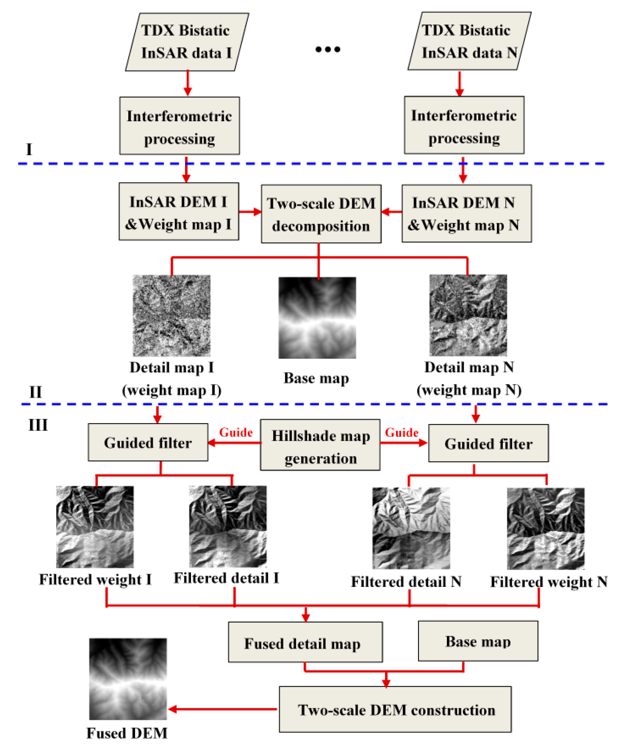
In this section, the methodology for the novel guided-filter-based InSAR DEM fusion algorithm is presented and analyzed based on the data processing sequence shown in Figure 1. This includes: (1) InSAR DEM generation and theoretical error analysis (Section 2.1); (2) InSAR DEM decomposition and hillshade map generation (Section 2.2); and (3) InSAR DEM fusion with guided filter (Section 2.3).
2.1. InSAR DEM Generation and Theoretical Error Analysis
As shown in part I of Figure 1, the surface elevation was measured by the interferometric phase and was then converted to height through the geometric relationship with the InSAR technique. The interferometric phase was calculated as the argument of the conjugate multiplication of two coregistered SAR images. As the master and slave images of the bistatic TanDEM-X interferometric pair were acquired simultaneously, there was no deformation phase, and the atmospheric phase could typically be neglected. Therefore, the interferometric phase ϕint comprised two components as follows [26]:
where is the phase linearly related to the topographic height to be determined, and is the phase caused by the thermal noise of the SAR sensor as well as the decorrelation between two SAR acquisitions whose impact can be mitigated through interferogram filtering.
The SRTM DEM was used as the reference DEM and radar coded into the image space of the interferogram. The reference topographic phase can be simulated from the radar-coded height as follows [27]:
where is the height ambiguity, is the wavelength, is the slant range, is the incidence angle, and is the vertical baseline. After the removal of the reference topographic phase, the fringes of the interferogram were evidently reduced and were thus easier to unwrap. Then, the residual phase signal in the differential interferogram was reasonably assumed to represent local topographic details that could not be portrayed by the reference DEM. In order to suppress the phase noise, Goldstein filtering [28,29] was performed on the differential interferogram before phase unwrapping. There are classic methods for phase unwrapping, such as the branch-cut method [30], the minimum cost flow (MCF) method [31], the statistical-cost network-flow approaches for phase unwrapping (SNAPHU) [32], etc. Considering both the effectiveness and efficiency of these methods, the MCF method was adopted for phase unwrapping in this study.
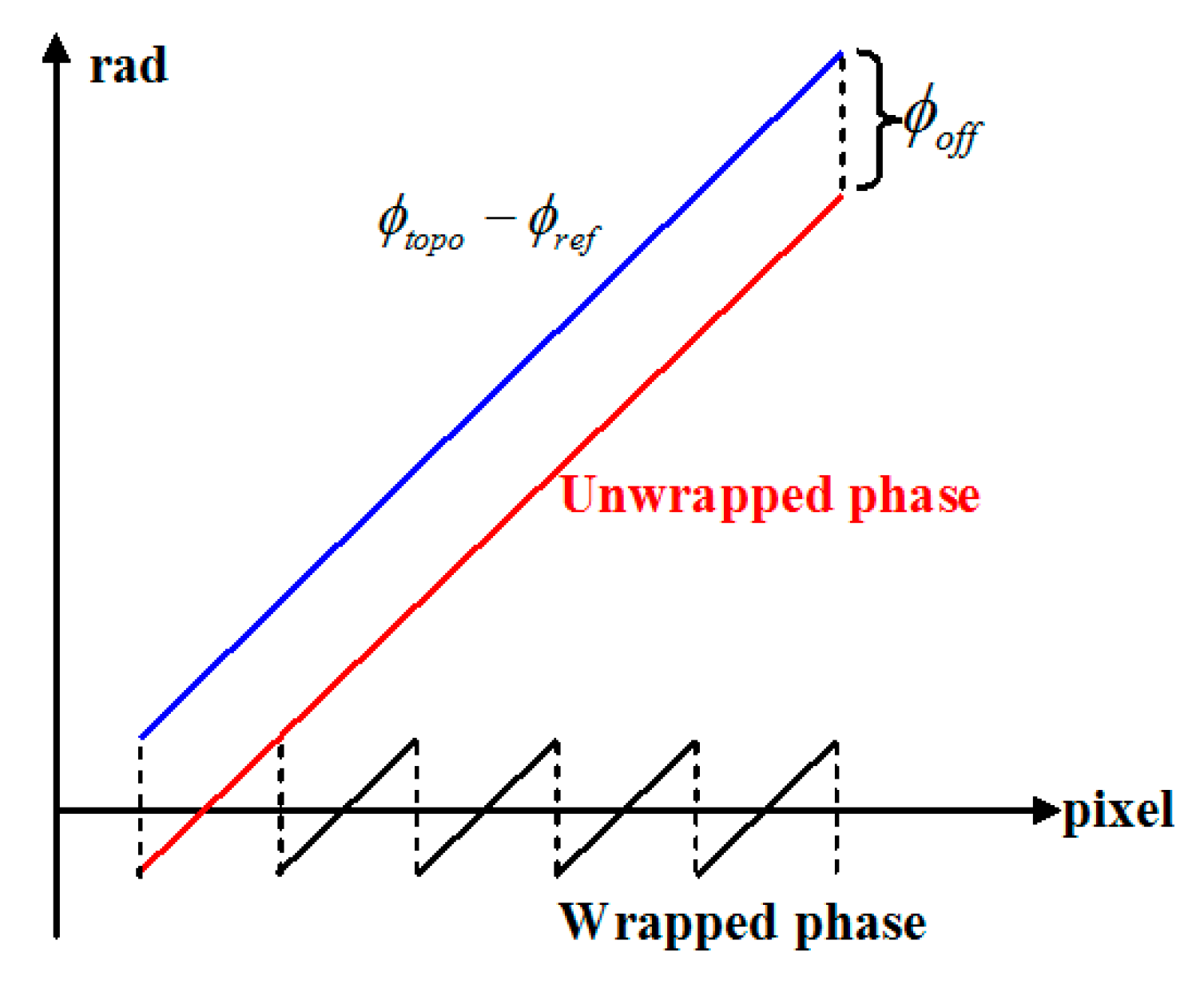
After the phase unwrapping of the differential interferogram, the unwrapped phase was represented by . The interferometric phase simulated from the reference DEM showed large-scale, low-frequency topographic information, while the unwrapped differential phase obtained above was considered to represent small-scale, high-frequency topographic information. Therefore, we could recover the full topographic phase by merging these two phase components together [33]. However, there always was an offset between the unwrapped differential phase and absolute differential phase , as shown in Figure 2, and a phase calibration process was therefore needed to determine this offset .
In this study, we selected sample points in the reference DEM in relatively flat areas with very small residual phase difference between the actual topographic phase and the reference topographic phase. The phase offset of the sample points can be written as:
In order to ensure calibration accuracy, observation samples were collected all over the images with theoretical height errors below an empirically set threshold. The absolute phase offset was determined through the weighted average of phase offset at the selected sample points, as given in Equation (4) below, with the weights calculated by Equation (5) below. Additionally, the weights were used for the InSAR DEM weighted average fusion.
After the absolute phase offset calibration, the topographic phase can be well reconstructed according to the following equation:
The standard deviation of the height error is an important factor to determine weights for absolute phase calibration as well as InSAR DEM fusion and can be estimated from the standard deviation of phase error [27]:
The remaining problem was how to estimate the standard deviation of the phase error . Reference [34] gives the conditional probability density function (PDF) of the interferometric phase as , where is the mathematical expectation of the interferometric phase , is the coherence coefficient, and is the effective look number. When is set as zero, describes the probability distribution of the interferometric phase noise [34]. Thus, the phase noise can be calculated by integrating the phase noise probability density function :
The InSAR height was calculated using the linear relationship between the topographic phase and the terrain height based on Equation (2). Subsequently, the InSAR estimated height , the theoretical height error , and the weight were all georeferenced and gridded in the geographic coordinate system (latitude and longitude) or projected coordinate system, e.g., Universal Transverse Mercator (UTM) system.
2.2. InSAR DEM Decomposition and Hillsade Map Generation
From the above section, the single-baseline InSAR DEM with corresponding theoretical height error was generated. In order to combine the meaningful information and fix the data voids, it is effective to fuse the multi-baseline and multi-orbit InSAR DEMs together. In this study, the edge-preserving smoothing guided filter was utilized for DEM fusion. This section acted as the preparation or preprocessing step for the subsequent InSAR DEM fusion with guided filtering corresponding to part II of Figure 1. The preprocessing included two major parts: InSAR DEM decomposition and hillshade map generation.
In order to better preserve details, the InSAR DEM is decomposed into two scales including the base map and the detail map, which correspond to the low-frequency rough terrain information and the high-frequency fine terrain details, respectively. In this study, the decomposition of the DEM was performed by a simple average filtering. First, the mean height map of all the input coregistered height layers was calculated. Then, the base map B could be obtained by the average filter for the mean height layer. Subsequently, the detail map was calculated by subtracting the base map B from the DEM.
However, terrain details are easily mixed with high-frequency noise information, and it is therefore challenging to preserve meaningful details and eliminate noise information. As meaningful detail information is closely related with terrain conditions, the hillshade map, which can greatly enhance the terrain features, was proposed to act as the guidance image during the guided filter processing. Thus, terrain features, such as ridges, could be well preserved. The hillshade map can evidently highlight the terrain features by calculating the hypothetical illumination of a surface [35].
2.3. InSAR DEM Fusion with Guided Filter
Guided filter belongs to the category of edge-preserving filters that can smooth noise and preserve details. The guided filter is based on a local linear model, the computing time of which is independent of the filter size. The guided filter is qualified for other applications such as image matting, up-sampling colorization [36], and image fusion [25]. In this study, the guided filter was first applied for InSAR DEM fusion corresponding to part III of Figure 1.
is used to represent the guided filtering operation, where parameters r and are the parameters that decide the filter size and blur degree of the guided filter, respectively, and P, I, and Q refer to the input image, guidance image, and output image, respectively. In this study, we used the hillshade map as the guidance image I, which could integrate terrain feature information into the fusion process. In Section 2.2, the InSAR DEM had been decomposited into the base layer B and detail layer . The weight map for the generated InSAR DEM could be calculated from the theoretical height error based on Equation (5). Therefore, the detail layer and the weight map were performed as input images. Following the guided filtering processing shown in Equations (9) and (10) below, the output images are the guided filtered detail map and weight map :
In theory, the guided filter assumes that the filtering out the filtering output is a linear transformation of the guidance image I in a local window centered at pixel k. There are pixels inside the window .
where are some linear coefficients assumed to be constant in local window . The window size used is . This local linear model ensures that has an edge only if I has an edge, as , which is the reason that the guided filter is the edge-preserving smoothing filter. To determine the linear coefficients , the difference between the output image maintaining the linear model in Equation (11) and the input image should be minimized. The cost function in the local window is given by:
where is a regularization parameter penalizing large . Equation (12) is the linear ridge regression model [37,38], and its solution is given by:
where and are the mean and variance of guidance image I in , is the number of pixels in , and is the mean of the input image in . Having obtained the linear coefficients , we computed the filtering output by Equation (11).
However, a pixel i is involved in all the overlapping windows that cover i, so the value of in Equation (11) is not identical when it is computed in different windows. A simple strategy is to average all the possible values of coefficient . After computing for all windows in the image, the filtering output is computed by:
where , .
After the calculation of guided filtered detail map and weight map , the final detail map is computed by the weighted average as follows:
The final fused DEM can be reconstructed by the two-scale image composed of the base layer B and the average-weighted detail layer after guided filtering, as follows:
After the guided filtering process, the characteristics of the terrain features in the hillshade map could be incorporated with the high-frequency detail map and weight map. In other words, the guided filter with the hillshade map as the guidance map introduced the terrain-condition-related information into the fusion process, making the guided filtering algorithm more adapted to the DEM fusion. Considering that the guided filter can smooth the noise inside the local window, the InSAR DEM fusion with guided filter can smooth the height error while preserving the meaningful details.
3. Results
3.1. Experimental Area and Data
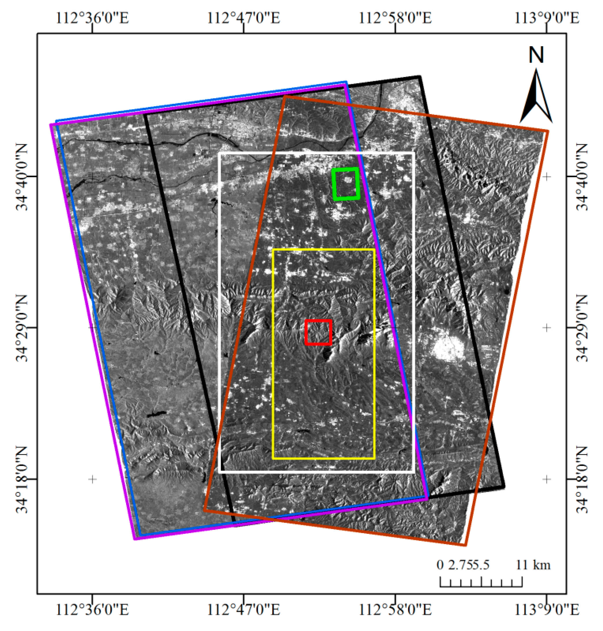
The test site was located at the junction of three cities in Henan province, China, namely, Zhengzhou, Luoyang, and Pingdingshan. Figure 3 shows the georeferenced amplitude image of a bistatic TanDEM-X InSAR pair from which it can be seen that the terrain types of the experimental area are diverse, including plains, hills, and mountains. The central part of the experimental area covered Mount Song, with elevations ranging from 150 m to 1500 m above sea level, and the slopes in the central part were very steep.
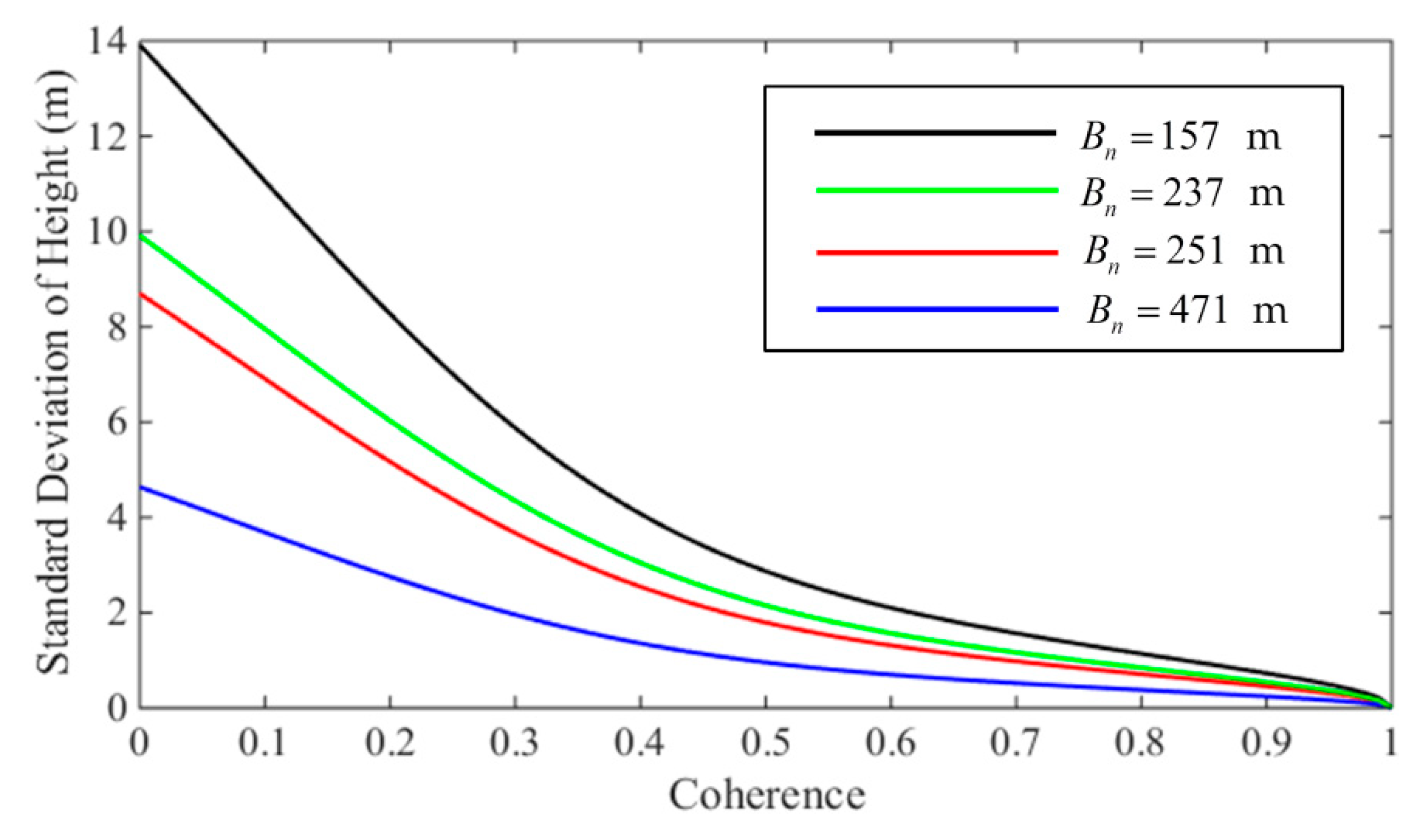
The TanDEM-X images used in this experiment were four stripmap bistatic InSAR pairs with different normal baselines. The detailed parameters of these InSAR pairs are shown in Table 1. It can be seen that the lengths of their normal baselines were 157, 237, 251, and 471 m and that the baselines were evenly distributed and were proper for the multi-baseline InSAR experiment. The SRTM DEM with 1 arc-second resolution covering our study area was used as a reference DEM for rough topographic phase removal in the InSAR processing.
In order to evaluate the height accuracy of the generated DEMs, a photogrammetric DEM of 1 m resolution was used as the reference elevation dataset. The photogrammetric DEM was acquired in 2011. The coverage of the photogrammetric DEM is marked by the white rectangle in Figure 3 inside the coverage of the TanDEM-X images marked by the black, purple, and brown rectangles in Figure 3. As mentioned in Reference [6], the height accuracy of the DEM product depends on the slope. The photogrammetric DEM used as reference DEM met the China Surveying and Mapping Industry Standard of 1:5000 resolution DEM, which means that for the flat terrain, the RMSE of the height error was less than 1 m, while for the mountainous areas, the RMSE was less than 5 m. There were different terrain types, such as mountains and plains, inside the coverage of the reference DEM, which made the reference DEM suitable for the evaluation of height accuracy in the generated DEMs in different kinds of terrain conditions.
We acquired the TanDEM-X DEM tile covering the test area through the annoucement of opportunity (AO) project of the German Aerospace Center. The TanDEM-X DEM is the global DEM product of the TanDEM-X mission. The TanDEM-X DEM acquisition phase took four years, from December 2010 to January 2015. The TanDEM-X DEM tile used in this study had an independent pixel spacing of 0.4 arcsec, which is about 12 m [39]. The absolute vertical accuracy of the TanDEM-X DEM is better than 10 m from the perspective of the 90% linear point-to-point error, which is defined as the 90th percentile of absolute height error with respect to zero [40,41]. After certain postprocessing of the TanDEM-X DEM, the commercial WorldDEMTM product can be produced, which consists of a digital surface model (DSM) representing the Earth’s surface (including heights of buildings and other man-made objects, trees, forests and other vegetation), and a digital terrain model (DTM) representing bare Earth; vegetation, and man-made objects are removed [42].
3.2. Experimental Results for InSAR DEM Fusion
The bistatic TanDEM-X InSAR data were processed to generate DEMs with different normal baselines based on the procedure presented in Section 2.1. The standard deviation of the height error was calculated based on Equation (7). The relationship between the standard deviation of the height error and coherence is plotted in Figure 4. It can be seen from Figure 4 that the height measurement accuracy was determined by the baseline length and coherence level. When the coherence was higher than 0.2, the theoretical standard deviation of the height error was no higher than 10 m. In order to control the phase unwrapping error, the coherence threshold for phase unwrapping was set to 0.2. After the interferometric processing, the single-baseline InSAR DEM was generated. The randomly distributed height error outliers determined by the 3 principle were eliminated to improve the height accuracy of the generated DEM.
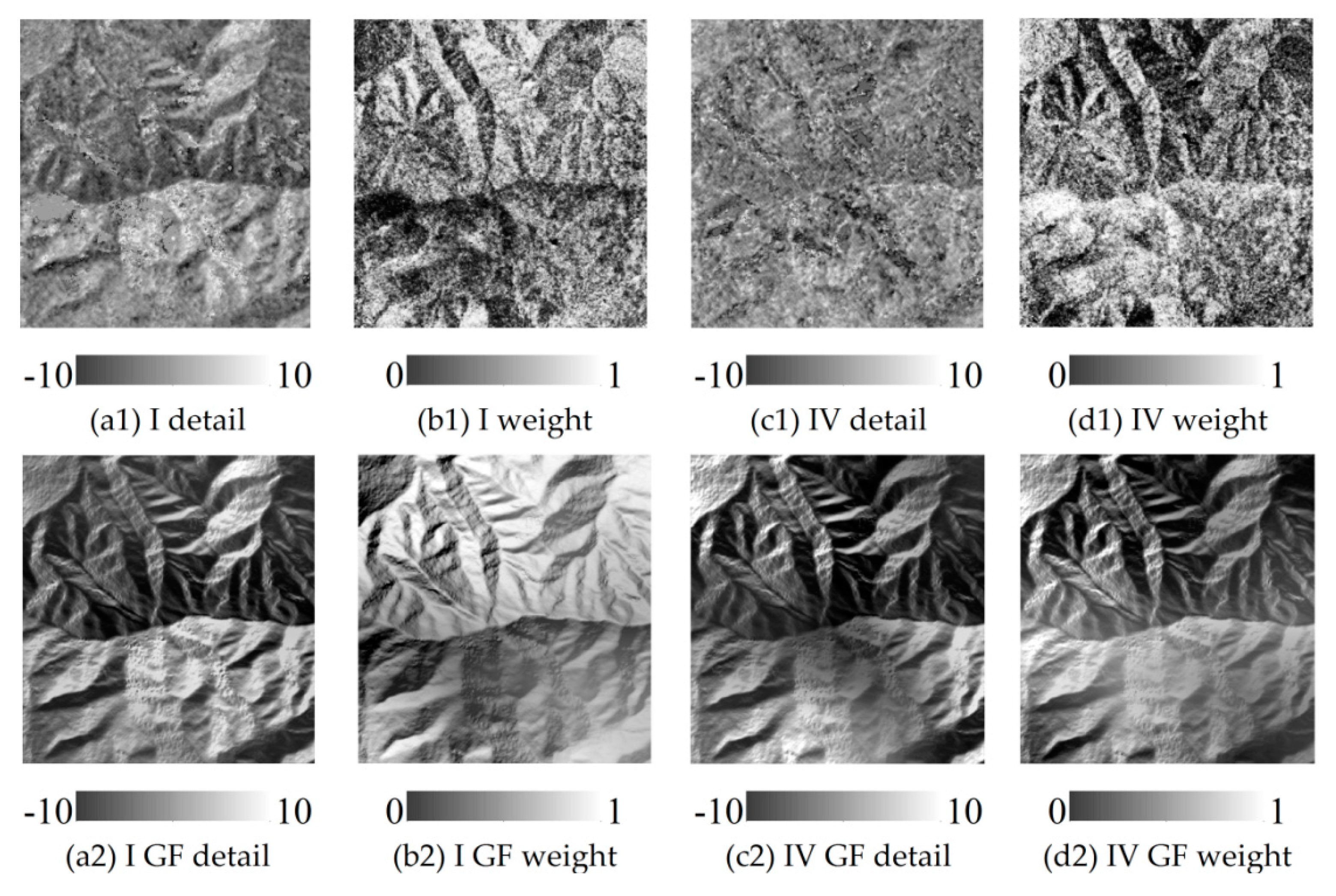
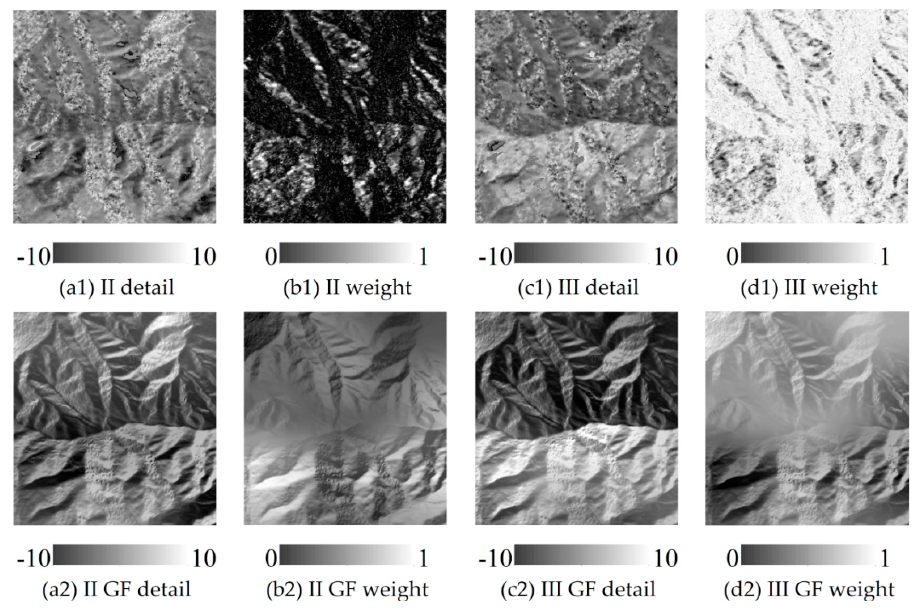
As well as fusion through guided filter, the single-baseline InSAR DEMs were also fused through weighted average as contrast experiment. The weight was determined by the theoretical height error as in Equation (7). As described in Section 2.2 and Section 2.3, the InSAR DEM to be fused was decomposited into a base layer and a detail layer. The averaged DEM of these InSAR DEMs was used to generate the hillshade image and the base image. The hillshade image enhanced the terrain features and was performed as the guidance image for the guided filtering of the detail image and weight image. Figure 5 and Figure 6 display the detail images and weight images before and after the guided filtering of the mountainous sample area marked by a red rectangle in Figure 3. The detail maps and weight maps of InSAR DEM I and IV are shown in Figure 5, and those of InSAR DEM II and III are shown in Figure 6. The first row and second row of Figure 5 and Figure 6 present the detail maps and weight maps before and after the guided filtering, respectively.
Analyzing the first row in Figure 5 and Figure 6, it can be seen that the detail map and weight map were related to the terrain features. Before the application of the guided filter, the images were full of “salt-and-pepper” noise. After the guided filtering, the detail maps and weight maps, shown in the second row of Figure 5 and Figure 6, could well integrate the terrain features. Additionally, as the guided filter could combine the local spatial context information, it could reduce the random noise information in the detail maps and weight maps.
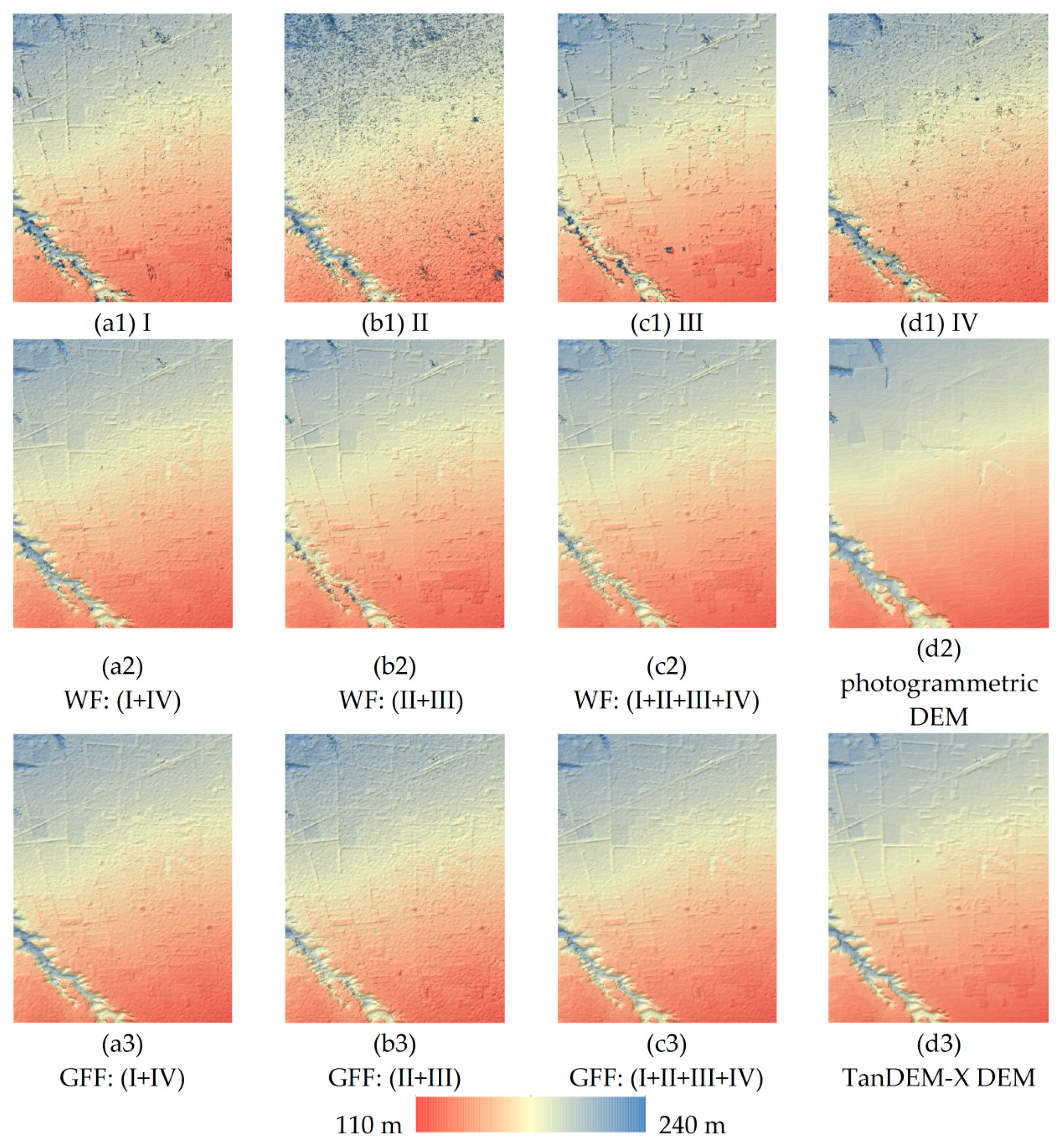
In order to well evaluate the fusion results for different terrain conditions, two sample areas—one plain area and one mountainous area—were selected, as marked by green and red rectangles in Figure 3 and presented as colored hillshade maps in Figure 7 and Figure 8. The single-baseline InSAR DEMs are presented in the first rows of Figure 7 and Figure 8. The weighted fused DEMs are shown in the second rows of Figure 7 and Figure 8. The fused DEMs with guided filter are shown in the third rows of Figure 7 and Figure 8.
Three different sets of experiments were used to assess the fusion methods. Subfigures a2 and a3 in Figure 7 and Figure 8 show the fused DEMs of InSAR DEM I ( m) and IV ( m); these represent the InSAR DEM fusion results with different orbital directions as interferogram I was acquired in the ascending direction and interferogram IV ( m) was acquired in the descending direction. Subfigures b2 and b3 in Figure 7 and Figure 8 display the fusion results of InSAR DEM II ( m) and III ( m); these represent the fused DEMs with different normal baseline lengths. Subfigures c2 and c3 in Figure 7 and Figure 8 are the fusion results of InSAR DEM I, II, III, and IV, which represent the fused multi-baseline and multi-orbit DEMs. The height accuracy was qualitatively evaluated by the photogrammetric DEM, and the statistical values of height error were calculated and are presented in Table 2. The DEM fusion process with weighted average or guided filter could fill in the data voids to some extent. Table 3 shows the number and percentage of the invalid pixels of the generated DEMs and can be used as an indicator to evaluate the effectiveness of the DEM fusion methods.
For the single-baseline InSAR DEMs—a1, b1, c1, and d1 in Figure 7 and Figure 8—there were data voids caused by geometric distortions or phase unwrapping errors. Comparing the InSAR DEMs I ( m, ascending) (a1) and IV ( m, descending) (d1) in Figure 7 and Figure 8, it could be found that the height surface at the toward-radar slopes was smoother and had fewer data voids than that at the back-radar slopes. In Table 2, the RMSEs of the single-baseline InSAR DEMs covering the whole test area, marked by the yellow rectangle in Figure 3, were all larger than 11 m. The RMSEs of the height at the two sample areas, marked by red and green rectangles in Figure 3, were all larger than 3 m. It is worth mentioning that the photogrammetric DEM used as the reference DEM in the plain sample area in subfigure d2 in Figure 7 did not contain as many terrain details as the InSAR DEMs. This is because the ground targets at the surface were eliminated when producing the photogrammetric DEM products.
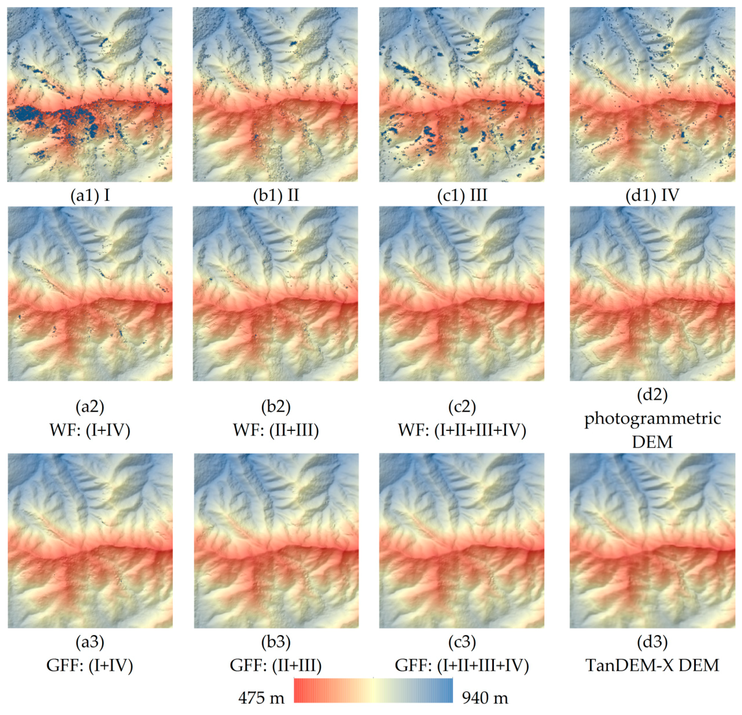
The fusion of ascending and descending InSAR DEMs could evidently compensate for geometric distortions caused by the data voids in the mountainous areas. The fused results, shown in subfigures a2 and a3 in Figure 8, could combine the useful information of both the toward-radar and back-radar slopes and fill in the data voids. Comparing a2 and a3 in Figure 8, the fused DEM with guided filter (a2) had fewer data voids and was smoother than the fused DEM with guided filter (a3). In Table 2, it can be seen that the RMSE of the fused DEM with weighted average filter, shown in Figure 8(a2), was 3.2 m, while the RMSE of the fused DEM with guided filter in Figure 8(a3) was 2.9 m. In Table 3, it can be seen that the percentage of invalid pixels at the mountainous sample area was 0.19% for the fused DEM with weighted average filter, while that for the fused DEM with guided filter was only 0.02%.
Subfigures c2 and d2 in Figure 8 are the fused DEMs of InSAR DEM II ( m) and III ( m) obtained using weighted average and guided filters, respectively. InSAR DEM III (c1), as shown in Figure 7 and Figure 8, had finer topographic details and less “salt-and-pepper” noise than InSAR DEM II (b1), also shown in Figure 7 and Figure 8. The fused DEMs with the weighted average and guided filter—as shown in subfigures b2 and c2, respectively, in Figure 7 and Figure 8—retained the terrain detail information and reduced the “salt-and-pepper” noise. In the mountainous sample area, the fused DEM with guided filter, as shown in Figure 8(b3), was smoother and had fewer data voids than the fused DEM with weighted average filter shown in Figure 8(b2). In Table 2, it can be seen that the RMSE of the fused DEM with weighted average filter, shown in Figure 8(b2), was 3.4 m, while the RMSE of the fused DEM with guided filter, shown in Figure 8(b3), was 2.8 m. In Table 3, for the whole test area, the percentage of invalid pixels was 0.69% for the weighted average and 0.02% for the guided filter. For the two sample areas, the percentage of invalid pixels was less than 0.2% for the weighted average and 0.02% for the guided filter.
Subfigures c2 and c3 in Figure 7 and Figure 8 display the fused DEM with InSAR DEMs I ( m, ascending), II ( m, ascending), III ( m, ascending), and IV ( m, descending) obtained using the weighted average and guided filters. In Table 3, it can be seen that the percentage of the invalid pixels was less than 0.26% for the fused DEM with weighted average filter and less than 0.02% for the fused DEM with guided filter covering the whole test area. In the plain and mountainous sample areas, there were no invalid pixels in the fused DEM with guided filter. The RMSE of the fused DEMs obtained using the weighted average and guided filters were 7.2 m and 6.7 m, respectively, both of which were superior to the TanDEM-X DEM, whose RMSE was 14.1 m. In the mountainous sample area, the RMSE of the fused DEM generated by weighted average filter was 3.1 m, while the RMSE of the fused DEM generated by guided filter was 2.6 m.
4. Discussion
The proposed DEM fusion method with guided filter was validated by three sets of experiments with the bistatic TanDEM-X data: ascending and descending InSAR DEM fusion, multi-baseline InSAR DEM fusion, and multi-baseline and multi-orbit InSAR DEM fusion. The most popularly applied InSAR DEM fusion method with weighted average filter was performed as a contrast experiment. The quality of the resultant DEMs was evaluated qualitatively from Figure 7 and Figure 8 and quantitatively from Table 2 and Table 3. The experimental results can be analyzed and discussed in terms of the following aspects.
4.1. Comparative Analysis of the Single-Baseline InSAR DEMs and the Fused InSAR DEMs
The InSAR DEM fusion strategy worked well for improving the DEM quality. The data voids in the single-baseline InSAR DEMs could evidently be reduced. Additionally, the InSAR DEM fusion could well retain the high-precision height information and reduce the height noise when fusing the multi-baseline and multi-orbit InSAR DEMs. Comparing InSAR DEM I ( m, ascending) (a1) with InSAR DEM IV ( m, descending) (d1) in Figure 8, the height accuracy in the mountainous areas of the DEMs was related to the slope orientation in that there were fewer data voids and less “salt-and-pepper” noise at the toward-radar slopes than the back-radar slopes. The fusion of InSAR DEMs with different orbital directions could compensate for the DEM data voids caused by the layover and shadow effects and preserve the high-precision height information at different slope sides. However, comparing InSAR DEM II ( m, ascending) (b1) with InSAR DEM III ( m, ascending) (c1) in Figure 8, the InSAR height measurement sensitivity increased with the normal baseline length; therefore, there were more detailed terrain features in the InSAR DEM with longer baseline, whereas the interferograms with longer normal baselines was more prone to phase unwrapping errors. The fusion of the InSAR DEMs with different normal baseline lengths could retain the high height measurement sensitivity of the long baseline and reduce the random height errors by increasing the numbers of observations.
4.2. Comparative Analysis of the Fused DEMs with Weighted Average and Guided Filters
Firstly, it can be seen from Figure 8 that the fused DEM with guided filter had fewer data voids than the fused DEM with weighted average filter for the whole test area, the plain sample area, and especially for the mountainous sample area. It can also be seen from Table 3 that for the whole test area, the percentage of invalid pixels was less than 0.71% for the fused DEM with weighted average filter and less than 0.03% for the fused DEM with guided filter. In mountainous sample areas, the percentage of invalid pixels was less than 0.2% for the weighted average filter and less than 0.02% for the guided filter, while in the plain area, the percentage was less 0.14% for the weighted average filter and less than 0.02% for the guided filter. This is due to the fact that the guided filter takes the local spatial context into consideration and that when there is an invalid pixel its value can be compensated by the neighboring pixels inside the search window; by contrast, the weighted average is only a pixel-based fusion and does not consider the neighboring height information. There were seldom any invalid pixels after the guided-filter-based DEM fusion. Another advantage of the addition of spatial neighborhood constraint information was that the fused DEM with guided filter was smoother and had less “salt-and-pepper” noise than the fused DEM with weighted average filter.
Secondly, the fusion method with guided filter could be seen to well preserve topographic features, such as ridges or boundaries. The guided-filter-based fusion method adopts a two-scale fusion strategy in which the InSAR DEMs that are to be fused are decomposited into a large-scale low-frequency base layer and a small-scale high-frequency detail layer. The guided-filter-based method focuses on small-scale terrain cues to preserve the details in the fusion process. Additionally, the hillshade map can enhance the terrain features and is used as guidance image for the weight map and detail map. Based on the edge-preserving characteristic of the guided filter, the edges and detail information of the guidance image can be retained and passed to the filtered image, and therefore the guided-filtered weight map and detail map are related to terrain features and are more helpful for preserving the terrain details.
It can be seen from Table 2 that the RMSEs of the fused DEM with guided filter were smaller than those of the fused DEM with weighted average filter, indicating that the DEM fusion method with guided filter was superior to the fusion method with weighted average filter.
4.3. Comparative Analysis of the Guided Filter and the Mean Filter
The mean filter provides a local spatial average of pixel values within a certain window and can reduce the random height error at the expense of resolution loss. The height accuracy improvement of the mean filter is limited to a certain extent as it can merely reduce the random height error, and with the loss of high-frequency meaningful detail information, the height accuracy can also be decreased.
Unlike the smooth operator mean filter, the guided filter is used as an edge-preserving smooth operator, as discussed in Section 2.1. It does not provide a local spatial average of pixel values but rather a local linear fit between the guidance image and input image. Therefore, the guidance image can be used as the constraint image. We used the hillshade map (with enhanced topographic features and generated from DEM) as a guidance image and accordingly we called it the terrain-guided filter. Because the local linear fit can maintain the local image gradient, the guided filter can well preserve the terrain details of the input image. The coefficients and of the linear conversion in Equation (11) are calculated through the average of all the possible values of and from all local windows covering the same pixel as in Equation (15). Thus, it can take the neighboring height information into consideration, which can help suppress the abnormal value.
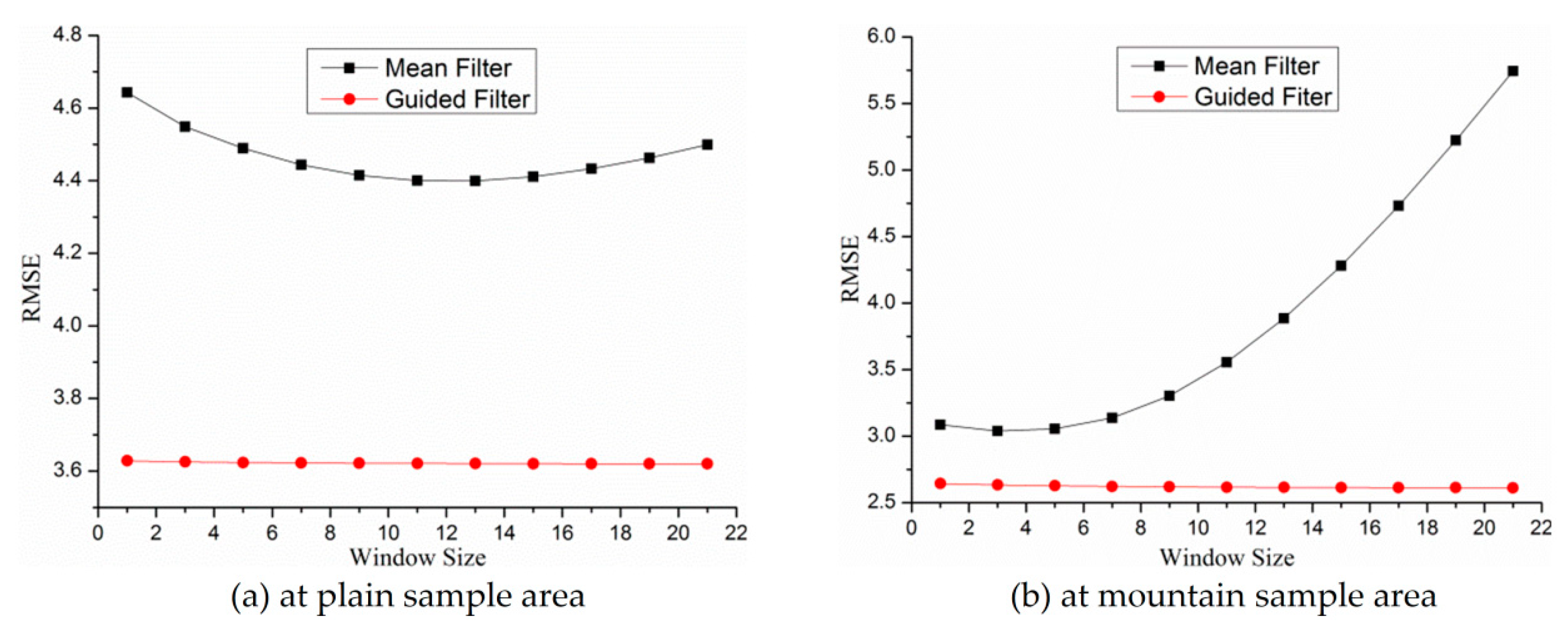
As contrast experiment, the mean filter was applied to the weighted averaged InSAR DEM. The RSME of the mean-filtered DEM was compared with the fused DEM with terrain-guided filter. For the mean filter, the local window size used is a very important parameter which determines the blur degree of the filtered DEM. Figure 9 shows the influence of the local window size on the height RMSE at plain and mountainous areas. It can be seen from Figure 9 that the local window size had evident influence on the RMSE of the filtered DEM. The RMSE first slightly decreased and then increased as window size increased on the whole. This is mainly due to the fact that the increase of local spatial information can effectively alleviate the effect of noise at the beginning. However, when the window size reaches a certain value, the RMSE tends to increase due to the oversmoothing effect. By contrast, for the fusion method based on terrain-guided filter, the RMSE level is little influenced by the window size, whether at plain sample area or mountainous sample area. The insensitivity of the guided filter has already been demonstrated by some studies [25,36]. Moreover, the RMSE of the fused DEM with terrain-guided filter was smaller than that of the weighted averaged DEM after mean filter, indicating the effectiveness of the proposed fusion method. Even though the RMSE was barely affected by the window size, we conservatively set the window size as 3 during the processing.
5. Conclusions
In this paper, a novel InSAR DEM fusion method with guided filter was developed and testified with the bistatic TanDEM-X InSAR data with different normal baselines and different orbital directions. The popularly applied InSAR DEM fusion method with weighted average was also adopted as a contrast experiment. Single-baseline and fused InSAR DEMs were generated, and their height accuracy was evaluated using photogrammetric DEM and TanDEM-X DEM. The main findings of this study are as follows:
- (1)
- The fusion of multi-baseline and multi-orbit InSAR DEMs can simultaneously solve the two major problems of single-baseline InSAR, namely the contradiction between height measurement sensitivity and phase unwrapping reliability caused by baseline length and the DEM data voids caused by layover or shadow effects. This technique maintains the advantage of higher height measurement sensitivity of long baselines while reducing the random height noise by increasing the number of observations. Furthermore, the fusion of ascending and descending InSAR DEMs can compensate for the data voids caused by geometric distortions.
- (2)
- The guided-filter-based InSAR DEM fusion method can take local spatial context information into consideration, which can help smooth the “salt-and-pepper” noise of InSAR DEMs and eliminate the abnormal height value. Furthermore, due to the spatial dependence of the height information, the guided-filter-based InSAR DEM fusion method can fill in almost all the data voids.
- (3)
- The guided-filter-based InSAR DEM fusion method can well preserve the terrain details. The two-scale fusion strategy can help retain the high-frequency detail information. Furthermore, the guided filter belongs to the category of edge-preserving smoothing filters, and the fused InSAR DEM obtained using guided filter can well preserve the terrain features with the DEM hillshade image as the guidance image.
- (4)
- The fused InSAR DEM with guided filter has smaller RMSE than the fused InSAR DEM with weighted average filter and the TanDEM-X DEM, which well validates the effectiveness of the proposed InSAR DEM fusion method with guided filter.
Author Contributions
Y.D. and B.L. performed the experiments and wrote the paper; L.Z. and M.L. analyzed the experiments and improved the paper; J.Z. designed and performed the experiments and improved the paper.
Funding
This work was financially supported by the National Key R&D Program of China (Grant No. 2017YFB0502700), the National Natural Science Foundation of China (Grant Nos. 61331016, 41774006, 41271457 and 41801280), Open Research Project of the Hubei Key Laboratory of Intelligent Geo-Information Processing (KLIGIP-2017B06), Open Fund of State Laboratory of Information Engineering in Surveying, Mapping and Remote Sensing, Wuhan University (Grant No. 17R01), and Fundamental Research Funds for the Central Universities, China University of Geosciences (Wuhan) under Grant CUG170676.
Acknowledgments
The authors would like to thank the German Aerospace Center (DLR) for providing the TanDEM-X CoSSC data via the DLR AO NTI_INSA6712 and the TanDEM-X DEM data via the DLR AO DEM_CALVAL0694. The authors would also like to thank Prof. Miaozhong Xu from LIESMARS for providing the photogrammetric DEM covering the Mount Song area for accuracy validation.
Conflicts of Interest
The authors declare no conflict of interest.
References
- Jiang, H.; Zhang, L.; Wang, Y.; Liao, M. Fusion of high-resolution DEMs derived from COSMO-SkyMed and TerraSAR-X InSAR datasets. J. Geod. 2014, 88, 587–599. [Google Scholar] [CrossRef]
- Zebker, H.A.; Goldstein, R.M. Topographic mapping from interferometric synthetic aperture radar observations. J. Geophys. Res.-Solid Earth 1986, 91, 4993–4999. [Google Scholar] [CrossRef]
- Zebker, H.A.; Werner, C.L.; Rosen, P.A.; Hensley, S. Accuracy of topographic maps derived from ERS-1 interferometric radar. IEEE Trans. Geosci. Remote Sens. 1994, 32, 823–836. [Google Scholar] [CrossRef] [Green Version]
- Rosen, P.A.; Hensley, S.; Joughin, I.R.; Li, F.K.; Madsen, S.N.; Rodriguez, E.; Goldstein, R.M. Synthetic aperture radar interferometry. Proc. IEEE 2000, 88, 333–382. [Google Scholar] [CrossRef] [Green Version]
- Rabus, B.; Eineder, M.; Roth, A.; Bamler, R. The shuttle radar topography mission—A new class of digital elevation models acquired by spaceborne radar. ISPRS J. Photogramm. Remote Sens. 2003, 57, 241–262. [Google Scholar] [CrossRef]
- Becek, K. Assessing Global Digital Elevation Models Using the Runway Method: The Advanced Spaceborne Thermal Emission and Reflection Radiometer Versus the Shuttle Radar Topography Mission Case. IEEE Trans. Geosci. Remote Sens. 2014, 52, 4823–4831. [Google Scholar] [CrossRef]
- Farr, T.G.; Rosen, P.A.; Caro, E.; Crippen, R.; Duren, R.; Hensley, S.; Kobrick, M.; Paller, M.; Rodriguez, E.; Roth, L. The shuttle radar topography mission. Rev. Geophys. 2007, 45, RG2004. [Google Scholar] [CrossRef]
- Krieger, G.; Moreira, A.; Fiedler, H.; Hajnsek, I.; Werner, M.; Younis, M.; Zink, M. TanDEM-X: A satellite formation for high-resolution SAR interferometry. IEEE Trans. Geosci. Remote Sens. 2007, 45, 3317–3341. [Google Scholar] [CrossRef] [Green Version]
- Fritz, T.; Rossi, C.; Yague-Martinez, N.; Rodriguez-Gonzalez, F.; Lachaise, M.; Breit, H. Interferometric processing of TanDEM-X data. In Proceedings of the 2011 IEEE International Geoscience and Remote Sensing Symposium (IGARSS), Vancouver, BC, Canada, 24–29 July 2011. [Google Scholar]
- Rizzoli, P.; Martone, M.; Gonzalez, C.; Wecklich, C.; Tridon, D.B.; Bräutigam, B.; Bachmann, M.; Schulze, D.; Fritz, T.; Huber, M. Generation and performance assessment of the global TanDEM-X digital elevation model. ISPRS J. Photogramm. Remote Sens. 2017, 132, 119–139. [Google Scholar] [CrossRef]
- Krieger, G.; Zink, M.; Bachmann, M.; Braeutigam, B.; Schulze, D.; Martone, M.; Rizzoli, P.; Steinbrecher, U.; Antony, J.W.; De Zan, F.; et al. TanDEM-X: A radar interferometer with two formation-flying satellites. Acta Astronaut. 2013, 89, 83–98. [Google Scholar] [CrossRef]
- Thompson, D.G.; Robertson, A.E.; Arnold, D.V.; Long, D.G. Multi-baseline interferometric SAR for iterative height estimation. In Proceedings of the 1999 IEEE International Geoscience and Remote Sensing Symposium, Hamburg, Germany, 28 June–2 July 1999. [Google Scholar]
- Pascazio, V.; Schirinzi, G. Multifrequency InSAR height reconstruction through maximum likelihood estimation of local planes parameters. IEEE Trans. Image Process. 2002, 11, 1478–1489. [Google Scholar] [CrossRef] [PubMed]
- Eineder, M.; Adam, N. A maximum-likelihood estimator to simultaneously unwrap, geocode, and fuse SAR interferograms from different viewing geometries into one digital elevation model. IEEE Trans. Geosci. Remote Sens. 2005, 43, 24–36. [Google Scholar] [CrossRef]
- Fornaro, G.; Guarnieri, A.M.; Pauciullo, A.; De-Zan, F. Maximum likelihood multi-baseline SAR interferometry. IEE Proc.-Radar Sonar Navig. 2006, 153, 279–288. [Google Scholar] [CrossRef]
- Dong, Y.; Jiang, H.; Zhang, L.; Liao, M. An Efficient Maximum Likelihood Estimation Approach of Multi-Baseline SAR Interferometry for Refined Topographic Mapping in Mountainous Areas. Remote Sens. 2018, 10, 454. [Google Scholar] [CrossRef]
- Xia, X.-G.; Wang, G. Phase unwrapping and a robust Chinese remainder theorem. IEEE Signal Process. Lett. 2007, 14, 247–250. [Google Scholar] [CrossRef]
- Ghiglia, D.C.; Wahl, D.E. Interferometric synthetic aperture radar terrain elevation mapping from multiple observations. In Proceedings of the IEEE 6th Digital Signal Processing Workshop, Yosemite National Park, CA, USA, 2–5 October 1994. [Google Scholar]
- Ferraiuolo, G.; Pascazio, V.; Schirinzi, G. Maximum a posteriori estimation of height profiles in InSAR imaging. IEEE Geosci. Remote Sens. Lett. 2004, 1, 66–70. [Google Scholar] [CrossRef]
- Ferretti, A.; Prati, C.; Rocca, F. Multibaseline InSAR DEM reconstruction: The wavelet approach. IEEE Trans. Geosci. Remote Sens. 1999, 37, 705–715. [Google Scholar] [CrossRef]
- Deo, R.; Rossi, C.; Eineder, M.; Fritz, T.; Rao, Y.S. Framework for Fusion of Ascending and Descending Pass TanDEM-X Raw DEMs. IEEE J. Sel. Topics Appl. Earth Observ. Remote Sens. 2015, 8, 3347–3355. [Google Scholar] [CrossRef]
- Gruber, A.; Wessel, B.; Martone, M.; Roth, A. The TanDEM-X DEM Mosaicking: Fusion of Multiple Acquisitions Using InSAR Quality Parameters. IEEE J. Sel. Topics Appl. Earth Observ. Remote Sens. 2016, 9, 1047–1057. [Google Scholar] [CrossRef]
- Shen, R.; Cheng, I.; Shi, J.; Basu, A. Generalized Random Walks for Fusion of Multi-Exposure Images. IEEE Trans. Image Process. 2011, 20, 3634–3646. [Google Scholar] [CrossRef] [PubMed]
- Li, S.Z. Markov random field models in computer vision. In Proceedings of the European Conference on Computer Vision, Stockholm, Sweden, 2–6 May 1994. [Google Scholar]
- Li, S.; Kang, X.; Hu, J. Image Fusion with Guided Filtering. IEEE Trans. Image Process. 2013, 22, 2864–2875. [Google Scholar] [PubMed]
- Ferretti, A.; Prati, C.; Rocca, F. Multibaseline phase unwrapping for InSAR topography estimation. Nuovo Cimento Della Soc. Ital. Fis. C 2001, 24, 159–176. [Google Scholar]
- Hanssen, R.F. Radar Interferometry: Data Interpretation and Error Analysis; Springer Science & Business Media: Berlin, Germany, 2001. [Google Scholar]
- Goldstein, R.M.; Werner, C.L. Radar interferogram filtering for geophysical applications. Geophys. Res. Lett. 1998, 25, 4035–4038. [Google Scholar] [CrossRef] [Green Version]
- Baran, I.; Stewart, M.; Lilly, P. A modification to the Goldstein radar interferogram filter. IEEE Trans. Geosci. Remote Sens. 2003, 41, 2114–2118. [Google Scholar] [CrossRef]
- Goldstein, R.M.; Zebker, H.A.; Werner, C.L. Satellite radar interferometry: Two-dimensional phase unwrapping. Radio Sci. 1988, 23, 713–720. [Google Scholar] [CrossRef]
- Costantini, M. A novel phase unwrapping method based on network programming. IEEE Trans. Geosci. Remote Sens. 1998, 36, 813–821. [Google Scholar] [CrossRef]
- Chen, C.W.; Zebker, H.A. Two-dimensional phase unwrapping with use of statistical models for cost functions in nonlinear optimization. JOSA A 2001, 18, 338–351. [Google Scholar] [CrossRef] [PubMed]
- Liao, M.; Jiang, H.; Wang, Y.; Wang, T.; Zhang, L. Improved topographic mapping through high-resolution SAR interferometry with atmospheric effect removal. ISPRS J. Photogramm. Remote Sens. 2013, 80, 72–79. [Google Scholar] [CrossRef]
- Tough, J.; Balcknell, D.; Quegan, S. A statistical description of polarimetric and interferometric synthetic aperture radar data. Proc. R. Soc. Lond. A 1995, 449, 567–589. [Google Scholar] [CrossRef]
- Burrough, P.A.; McDonnell, R.; McDonnell, R.A.; Lloyd, C.D. Principles of Geographical Information Systems; Oxford University Press: Oxford, UK, 2015. [Google Scholar]
- He, K.; Sun, J.; Tang, X. Guided Image Filtering. IEEE Trans. Pattern Anal. Mach. Intell. 2013, 35, 1397–1409. [Google Scholar] [CrossRef] [PubMed]
- Friedman, J.; Hastie, T.; Tibshirani, R. The Elements of Statistical Learning; Series in statistics; Springer: New York, NY, USA, 2001; Volume 1. [Google Scholar]
- Draper, N.R.; Smith, H. Applied Regression Analysis; John Wiley and Sons: New York, USA, 2014. [Google Scholar]
- Rizzoli, P.; Bräutigam, B.; Kraus, T.; Martone, M.; Krieger, G. Relative height error analysis of TanDEM-X elevation data. ISPRS J. Photogramm. Remote Sens. 2012, 73, 30–38. [Google Scholar] [CrossRef] [Green Version]
- Wecklich, C.; Gonzalez, C.; Braeutigam, B.; Rizzoli, P. Height Accuracy and Data Coverage Status of the Global TanDEM-X DEM. In Proceedings of the 11th European Conference on Synthetic Aperture Radar (EUSAR 2016), Hamburg, Germany, 6–9 June 2016. [Google Scholar]
- Wessel, B. TanDEM-X Ground Segment–DEM Products Specification Document; Technique Note 3.1; Ger. Aerosp. Center (DLR): Wessling, Germany, 2016. [Google Scholar]
- Becek, K.; Koppe, W.; Kutoğlu, Ş. Evaluation of Vertical Accuracy of the WorldDEM™ Using the Runway Method. Remote Sens. 2016, 8, 934. [Google Scholar] [CrossRef]
Figure 1.
Flowchart for the interferometric synthetic aperture radar digital elevation model (InSAR DEM) fusion with guided filter method.
Figure 1.
Flowchart for the interferometric synthetic aperture radar digital elevation model (InSAR DEM) fusion with guided filter method.

Figure 2.
Absolute phase offset calibration.

Figure 3.
The coverage of the TanDEM-X data is represented by purple (acquired on 19 October 2011 and 26 January 2012), black (20 July 2012), and brown (25 January 2014) rectangles in the georeferenced amplitude images. The photogrammetric DEM is marked by the white rectangle. The green and red rectangles show the plain and mountain sample areas, respectively. The yellow rectangle shows the common coverage area of the InSAR DEMs and reference DEM with different terrain types.

Figure 4.
Standard deviation of height error over all coherence intervals for different normal baselines.
Figure 4.
Standard deviation of height error over all coherence intervals for different normal baselines.

Figure 5.
Detail maps and weight maps of Interferograms I ( m, ascending) and IV ( m, descending). (a1,a2) and (b1,b2) are the detail maps and weight maps of Interferogram I, respectively; (c1,c2) and (d1,d2) are the detail maps and weight maps of Interferogram IV, respectively; (a1,b1,c1,d1) are the original detail maps and weight maps; and (a2,b2,c2,d2) are the guided filtered detail maps and weight maps.

Figure 6.
Detail maps and weight maps of Interferogram II ( m, ascending) and III ( m, ascending). (a1,a2) and (b1,b2) are the detail maps and weight maps of Interferogram II, respectively; (c1,c2) and (d1,d2) are the detail maps and weight maps of Interferogram III, respectively; (a1,b1,c1,d1) are the original detail maps and weight maps; and (a2,b2,c2,d2) are the guided filtered detail maps and weight maps.

Figure 7.
DEM magnifications of the plain area. (a1–a4) correspond to single-baseline InSAR DEMs I ( m), II ( m), III ( m), and IV ( m), respectively. (a2,a3) are the fused DEMs of I and IV; (b2,b3) are the fused DEMs of II and III; (c2,c3) are the fused DEMs of I, II, III, and IV; (a2,b2,c2) are fused by weighted average; and (a3,b3,c3) are fused by guided filter. The cell sizes of (a1–a3,b1–b3,c1–c3,d1) are 5 m. (d2) is the photogrammetric DEM with a cell size of 1 m and (d3) is the TanDEM-X DEM with a cell size of 12 m. The spatial dimension of each subfigure is about 2.3 km in width by 4.1 km in height.

Figure 8.
DEM magnifications of the mountainous area. (a1–a4) correspond to the single-baseline InSAR DEMs I ( m), II ( m), III ( m) and IV ( m), respectively. (a2,a3) are the fused DEMs of I and IV; (b2,b3) are the fused DEMs of II and III; (c2,c3) are the fused DEMs of I, II, III, and IV; (a2,b2,c2) are fused by weighted average; (a3,b3,c3) are fused by guided filter. The cell sizes of (a1–a3,b1–b3,c1–c3,d1) are 5 m. (d2) is the photogrammetric DEM with a cell size of 1 m; (d3) is the TanDEM-X DEM with a cell size of 12 m. The spatial size of each subfigure is about 2.6 km in width by 3.1 km in height.

Figure 9.
Analysis of the influence of window size on height root mean square error (RMSE) at different sample areas.
Figure 9.
Analysis of the influence of window size on height root mean square error (RMSE) at different sample areas.


Table 1.
Parameters for bistatic TanDEM-X interferometric pairs.
| Interferogram I | Interferogram II | Interferogram III | Interferogram IV | |
|---|---|---|---|---|
| Acquisition time | 19 October 2011 | 26 January 2012 | 20 July 2012 | 25 January 2014 |
| Orbit direction | Ascending | Ascending | Ascending | Descending |
| Imaging mode | Stripmap | Stripmap | Stripmap | Stripmap |
| Polarization | HH | HH | HH | HH |
| Normal baseline | 251 m | 157 m | 471 m | 237 m |
| Height ambiguity | 30 m | 48 m | 16 m | 34 m |
| Central incidence angle | 44.4° | 44.4° | 45.0° | 46.7° |
| Mean coherence coefficient | 0.82 | 0.75 | 0.73 | 0.84 |
Table 2.
Statistical values of height errors with respect to the photogrammetric digital elevation model (DEM) (unit: m).
Table 2.
Statistical values of height errors with respect to the photogrammetric digital elevation model (DEM) (unit: m).
| All | Plain | Mountain | ||||||||
|---|---|---|---|---|---|---|---|---|---|---|
| Mean | RMSE | 90% LE | Mean | RMSE | 90% LE | Mean | RMSE | 90% LE | ||
| IV | m | 4.8 | 14.0 | 24.2 | 2.3 | 3.5 | 6.1 | −0.9 | 7.8 | 13.5 |
| III | m | 3.9 | 11.3 | 19.6 | 2.0 | 3.8 | 6.6 | −0.8 | 3.9 | 6.8 |
| II | m | 4.2 | 14.0 | 24.2 | 4.1 | 6.6 | 11.4 | 0.1 | 5.2 | 9.0 |
| I | m | 3.7 | 13.5 | 23.4 | 3.0 | 3.4 | 5.9 | 2.6 | 3.4 | 5.9 |
| I + IV | WF | 4.4 | 9.1 | 15.8 | 2.6 | 3.2 | 5.5 | 1.1 | 3.2 | 5.5 |
| GFF | 4.7 | 7.1 | 12.3 | 2.4 | 3.1 | 5.4 | 0.4 | 2.9 | 5.0 | |
| II + III | WF | 4.2 | 9.4 | 16.3 | 3.8 | 5.9 | 10.2 | −0.2 | 3.4 | 5.9 |
| GFF | 4.2 | 6.8 | 11.8 | 3.0 | 4.6 | 8.0 | −0.4 | 2.8 | 4.8 | |
| I + II + III + IV | WF | 4.3 | 7.2 | 12.5 | 3.4 | 4.6 | 8.0 | 0.4 | 3.1 | 5.4 |
| GFF | 4.4 | 6.7 | 11.6 | 2.8 | 3.7 | 6.4 | 0.3 | 2.6 | 4.5 | |
| TanDEM-X DEM | 1.6 | 14.1 | 24.4 | 1.6 | 3.5 | 6.1 | 0.3 | 3.1 | 5.4 | |
Table 3.
Number and percentage of the invalid cells in the DEM.
| All | Plain | Mountain | |||||
|---|---|---|---|---|---|---|---|
| Num. | Percentage | Num. | Percentage | Num. | Percentage | ||
| I | m | 378,026 | 2.04 | 4912 | 0.91 | 13518 | 5.81 |
| II | m | 291,784 | 1.58 | 12752 | 2.35 | 2220 | 0.95 |
| III | m | 395,605 | 2.14 | 4797 | 0.89 | 9010 | 3.87 |
| IV | m | 331,015 | 1.79 | 5094 | 0.94 | 3063 | 1.32 |
| I + IV | WF | 131,861 | 0.71 | 492 | 0.09 | 431 | 0.19 |
| GFF | 4997 | 0.03 | 62 | 0.01 | 54 | 0.02 | |
| II + III | WF | 128,201 | 0.69 | 732 | 0.14 | 251 | 0.11 |
| GFF | 4486 | 0.02 | 93 | 0.02 | 13 | 0.006 | |
| I + II + III + IV | WF | 48,253 | 0.26 | 72 | 0.01 | 8 | 0.003 |
| GFF | 3431 | 0.02 | 1 | 0 | 0 | 0 | |
© 2018 by the authors. Licensee MDPI, Basel, Switzerland. This article is an open access article distributed under the terms and conditions of the Creative Commons Attribution (CC BY) license (http://creativecommons.org/licenses/by/4.0/).
Share and Cite
MDPI and ACS Style
Dong, Y.; Liu, B.; Zhang, L.; Liao, M.; Zhao, J. Fusion of Multi-Baseline and Multi-Orbit InSAR DEMs with Terrain Feature-Guided Filter. Remote Sens. 2018, 10, 1511. https://doi.org/10.3390/rs10101511
AMA Style
Dong Y, Liu B, Zhang L, Liao M, Zhao J. Fusion of Multi-Baseline and Multi-Orbit InSAR DEMs with Terrain Feature-Guided Filter. Remote Sensing. 2018; 10(10):1511. https://doi.org/10.3390/rs10101511
Chicago/Turabian StyleDong, Yuting, Baobao Liu, Lu Zhang, Mingsheng Liao, and Ji Zhao. 2018. "Fusion of Multi-Baseline and Multi-Orbit InSAR DEMs with Terrain Feature-Guided Filter" Remote Sensing 10, no. 10: 1511. https://doi.org/10.3390/rs10101511
Note that from the first issue of 2016, this journal uses article numbers instead of page numbers. See further details here.