Article

Mapping Maize Evapotranspiration at Field Scale Using SEBAL: A Comparison with the FAO Method and Soil-Plant Model Simulations

1
Mario Gulich Institute, National Agency of Spatial Activities (CONAE), X5000 Córdoba, Argentina
2
Institute of Environmental Engineering, ETH Zurich, 8093 Zurich, Switzerland
3
Department of Agronomy, Food, Natural Resources, Animals and Environment, University of Padova, 35020 Legnaro PD, Italy
4
Harvesting, Silicon Valley, CA 94027, USA
5
INTA EEA Manfredi, 5988 Córdoba, Argentina
6
Department of Civil, Environmental and Architectural Engineering, University of Padova, 35131 Padova, Italy
*
Author to whom correspondence should be addressed.
Remote Sens. 2018, 10(9), 1452; https://doi.org/10.3390/rs10091452
Submission received: 8 July 2018 / Revised: 3 September 2018 / Accepted: 7 September 2018 / Published: 11 September 2018
(This article belongs to the Special Issue Remote Sensing of Evapotranspiration (ET))

Abstract

:
The surface energy balance algorithm for land (SEBAL) has been successfully applied to estimate evapotranspiration (ET) and yield at different spatial scales. However, ET and yield patterns have never been investigated under highly heterogeneous conditions. We applied SEBAL in a salt-affected and water-stressed maize field located at the margin of the Venice Lagoon, Italy, using Landsat images. SEBAL results were compared with estimates of evapotranspiration by the Food and Agriculture Organization (FAO) method (ETc) and three-dimensional soil-plant simulations. The biomass production routine in SEBAL was then tested using spatially distributed crop yield measurements and the outcomes of a soil-plant numerical model. The results show good agreement between SEBAL evapotranspiration and ETc. Instantaneous ET simulated by SEBAL is also consistent with the soil-plant model results (R2 = 0.7047 for 2011 and R2 = 0.6689 for 2012). Conversely, yield predictions (6.4 t/ha in 2011 and 3.47 t/ha in 2012) are in good agreement with observations (8.64 t/ha and 3.86 t/ha, respectively) only in 2012 and the comparison with soil-plant simulations (8.69 t/ha and 5.49 t/ha) is poor. In general, SEBAL underestimates land productivity in contrast to the soil-plant model that overestimates yield in dry years. SEBAL provides accurate predictions under stress conditions due to the fact that it does not require knowledge of the soil/root characteristics.

Graphical Abstract

1. Introduction

The growing world population needs more food, possibly with less water available for agriculture [1], making the wise management of water resources one of the great challenges of our times. This problematic situation can improve only if water is managed more effectively leading to increased crop yield per unit of water consumed (i.e., improving water use efficiency). In arid and semiarid regions cropland irrigation is the major consumer of water and efficient and reliable methods for determining water consumption by crops are crucial for sustainable management [2,3,4,5]. Evapotranspiration (ET) is the largest sink of irrigation water and, thanks to well-established crop-specific relations between ET and yield [6,7], it provides a measure of both water demand and land productivity. Yield is thus the ultimate indicator to describe crop response to water resource management [8] and the quantification of field scale ET is fundamental for managers to maximize land productivity while minimizing water losses [9,10,11]. Crop yield is also a key element for rural development and national food security. For these reasons, forecasting crop yield a few months before harvest can be of paramount importance for timely initiation of the food trade, securing national demand, and organizing food transport within countries [6,7,12].
The yield of many agricultural crops is generally predicted from the amount of water used by the crop, i.e., ET [6,7]. Traditionally, ET from fields has been estimated according to the Food and Agriculture Organization (FAO) method [13], i.e., by multiplying a weather-based reference ET0 by a crop coefficient (Kc) determined according to crop type and growth stage. However, the suitability of the idealized Kc coefficient to describe the actual vegetative and growing conditions, especially in water limited areas, was questioned by many authors [14]. In addition, it is difficult to predict the correct growth stage dates for large populations of crops and fields [15].
A viable alternative for mapping evaporation at field and regional scales is the use of satellite images that can provide an excellent tool to detect the spatial and temporal structure of ET [16]. Remote sensing (RS) is a reliable and cost-effective method to forecast crop ET and yield over large areas [17,18] and the integrated use of remote-sensing data and crop modeling for yield prediction has been applied for many years [18]. Applications can be found in the literature for different crop types and regions using various data assimilation schemes [19,20,21]. However, these applications are based on medium resolution satellite data (MODIS, MERIS) and valid for regional assessments only [18]. Common RS models are the surface energy balance algorithm for land (SEBAL; [22]), mapping evapotranspiration at high resolution with internalized calibration (METRIC; [15]), remote sensing of evapotranspiration (ReSET; [23]), analytical land atmosphere radiometer model (ALARM; [24]) and surface aerodynamic temperature ([25]). Most of these models use the land surface energy balance equation:
R n = L E + G + H
where Rn is net radiation, LE is the latent heat flux, G is the soil heat flux and H is the sensible heat flux. When using satellite imagery, the sensed surface radiances are converted into surface properties such as albedo, vegetation indices, surface emissivity and surface temperature. These products are then used to estimate the various components of Equation (1) [26].
SEBAL is capable of estimating ET (from the latent heat flux) without prior knowledge of the soil, crop and management conditions [27], and it has been used to estimate the surface energy fluxes at different spatial and temporal resolutions in more than 30 countries [27,28,29,30] ET estimated by SEBAL has been utilized to quantify spatial variation of soil moisture [31], biomass production and crop yield [6] using high- and low-resolution satellite images within a field, across fields, and at regional scale [32]. The energy balance model in SEBAL uses a near-surface temperature gradient, dT, which eliminates the need for absolute surface temperature calibration, a “major stumbling block in operational satellite ET” [15]. Typical accuracies of the estimated ET by SEBAL are 85%, 95%, and 96% at daily, seasonal and annual timescales, respectively [27,30]. The advantages of using SEBAL have already been highlighted by [30]: (1) it uses minimal ground-based data; (2) calculation of the near-surface air temperature is not mandatory; and (3) a self-calibration process is automated in each region of interest. Despite a recent version of SEBAL model (SEBAL2008) having incorporated major refinements, such as correction of the advection effect or improved estimates of surface albedo and soil heat flux [33], the ability of SEBAL to describe ET and yield patterns at field scale has never been tested under highly heterogeneous conditions. The purpose of this study is to apply SEBAL for calculating ET in a salt-affected and water-stressed maize field located at the margin of the Venice Lagoon, Italy. SEBAL results are compared with ET estimates by the FAO method and the outcome of a three-dimensional soil-plant model. The biomass production routine in SEBAL is then tested using spatially distributed crop yield measurements and the soil-plant model results.

2. Materials and Methods
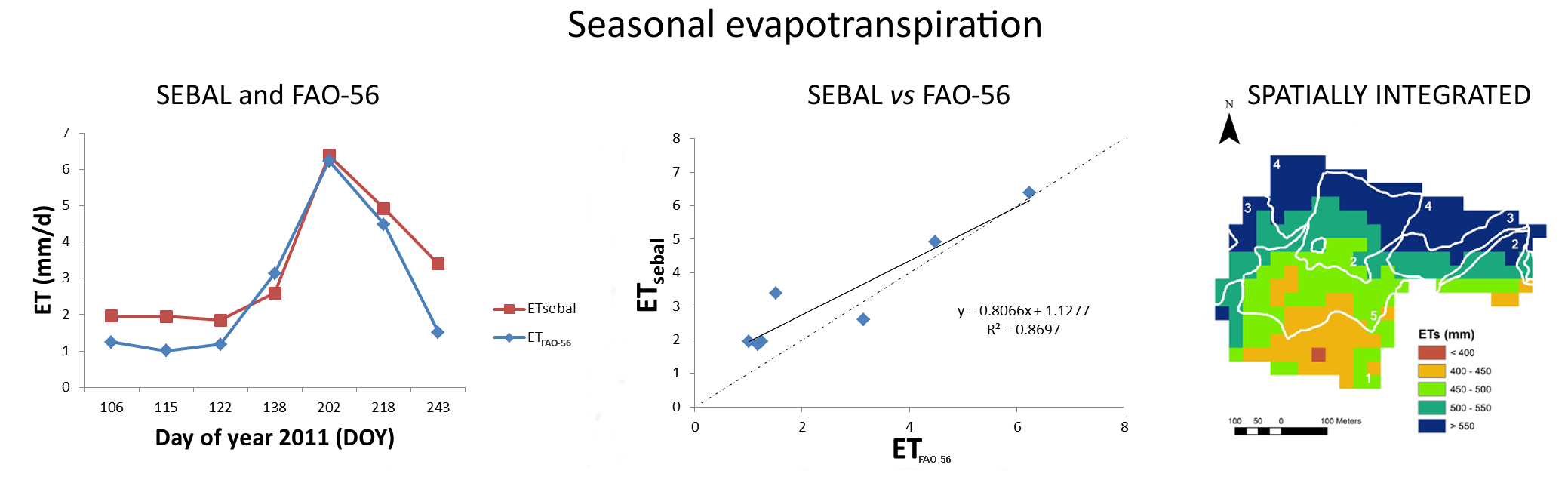
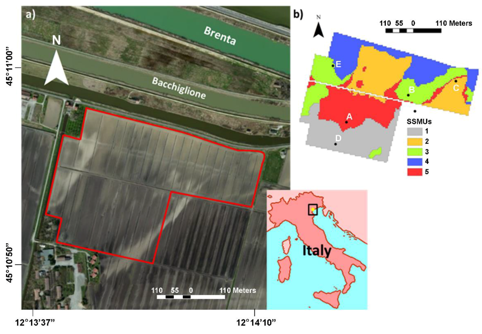
2.1. Study Area

The study site (Figure 1) is a ca. 21 ha field located in Ca’ Bianca (45°10′57″N, 12°13′55″E), near the town of Chioggia (Italy) at the southern margin of the Venice Lagoon. The area is in proximity to the Brenta and Bacchiglione Rivers and approximately 5 km from the Adriatic Sea. With an elevation ranging between 1 and 3.3 m below mean sea level, the site has a silt-clay soil with peat and sandy drifts (i.e., paleochannels) [34,35] (Figure 2). The area is known to be affected by saltwater contamination down to about 20 m depth with the presence of a first confined fresh-water aquifer 45–50 m below mean sea level. The climate is continental with annual rainfall around 780 mm. Rainfall is more intense in spring and autumn and snow is not very frequent during winter. The average daily temperature is 13.4 °C. Rainfed maize (Zea mais L.) was cultivated in 2011 (seeding 4 April and harvest 2 September), and 2012 (seeding 21 March and harvest 11 September). Precipitation differed substantially over the two growing seasons and was also quite unusual with respect to the average April-to-September rainfall from 1993 to 2012, which amounts to 360 mm. Indeed, the two growing seasons were rather dry (i.e., in the 1st quartile, 199.8 mm in 2011, 150.6 mm in 2012). Rainfall in 2011 was evenly spread throughout the season. Contrarily, the low 2012 precipitation occurred almost exclusively during the maize vegetative phase. No precipitation occurred during the early tassel and kernel blister reproductive stages, which are known to be among the most critical stages of maize growth [36]. The daily average reference evapotranspiration (ET0) was 4.42 and 4.08 mm d–1, whereas the ET0 over the entire season was 672 and 717 mm in 2011 and 2012, respectively. The study site was divided into five site-specific management units (SSMUs, Figure 1b) by [35] according to the spatial variability of soil characteristics and salinity (Figure 2) and has been extensively studied by soil sampling, hydro-geophysical monitoring and soil-plant modeling [34,35,36,37,38]. More precisely, the classification identified a peaty, acidic, moderately saline and sandy zone (SSMU 1); a very saline zone (SSMU 2); a non-saline zone comprising the coarser portions of the paleochannels (SSMU 3); a zone with the best conditions for maize growth (SSMU 4) with mid to low salinity, mid to low peat content and the highest clay content; and a peaty, acidic, moderately saline and silty zone (SSMU 5) (Figure 3).

2.2. Data

2.2.1. Acquisition of Satellite Imagery

Satellite images of the study area were obtained from Landsat 7 ETM+ (Path = 192, Row = 029). These images are made publicly available by the U.S. Geological Survey (at http://glovis.usgs.gov/USGS) as GeoTIFF with a level correction 1T (terrain corrected), providing a systematic radiometric and geometric accuracy through the use of point ground control (GCPs). For 2011, images were available for the dates 16 and 25 April, 2 and 18 May, 21 July, 6 and 31 August, while for 2012 the images were obtained on 18 and 27 April, 4 May, 5 June, 7 and 16 July, 1, 8, 17 August and 9 September. All dates had favorable clear-sky weather conditions. Visible bands (bands 1–5, 7) were used for albedo (α), and vegetation index calculations. Albedo was calculated by integrating surface reflectivity values, using different weighting coefficients for each band [2]. A “top of atmosphere” bidirectional reflectance was converted into at-surface reflectance, by using simple humidity and sun-angle based algorithms [39]. This simple approach for atmospheric correction could originate errors in albedo, which are anyway compensated by the internal calibration procedures of SEBAL [40]. Thermal band (band 6) was used for surface temperature (Ts), computed using a modified Plank equation following [41], and sensible heat (H). The spatial resolution is 30 × 30 m on the visible bands and 60 × 60 m on the thermal band.
Due to the presence of gaps in ETM+7 scan-line corrector (SLC)–off, only images covering 100% of the study area were considered. We decided not to fill the Landsat 7 gaps to avoid the risk of generating additional uncertainties. Seasonal ET was calculated from the Landsat images using the method for temporal integration implemented in the Geographic Resources Analysis Support System Geographic Information System (GRASS GIS 7) [42].

2.2.2. Hydrological Monitoring

To assess the impact of water stress on crop productivity, five monitoring stations were set up in the study site. Each station was equipped with capacitance-resistance probes (ECH2O-5TE, Decagon Devices, Pullman, WA, USA) to measure water content and pore-water salinity [38], and electronic tensiometers (T4e, UMS GmbH, Munich, Germany) to record soil-water potential at 10, 30, 50, and 70 cm depths. The sensors were connected to a data logger and recorded hourly. The water table level at each station was monitored every second week using phreatic wells. The five monitoring stations were named A, B, C, D and E (Figure 1b). Unfortunately, since the SSMUs were defined after station installation, SSMU 4 was not monitored by any of the stations, whereas two stations (B and E) were located in SSMU 3.

2.2.3. Meteorological Data and Estimation of Evapotranspiration by the Food and Agriculture Organization (FAO) Method (ETc)

In addition to satellite images, the SEBAL model requires the following input data: wind speed, precipitation, air humidity (vapor pressure or dew point temperature), solar radiation, air temperature, ET0, and meteorological station characteristics (height of wind measurement and vegetation height). Hourly meteorological data were acquired from a nearby automatic station (Regional Agency for Environmental Protection and Prevention of the Veneto) and used to calculate the reference evapotranspiration ET0 with the FAO-56 method [13]. Crop evapotranspiration (ETc), which differs distinctly from ET0 as it accounts for crop-specific ground cover, canopy properties and aerodynamic resistance, is then estimated by means of the crop coefficient Kc, as ETc = Kc × ET0 [13].
Where field conditions differ from the standard conditions, correction factors are required to adjust ETc. This adjustment reflects the fact that the real crop evapotranspiration often deviates from ETc due to non-optimal field conditions such as the presence of pests and diseases, soil salinity, low soil fertility, water shortage or waterlogging. The crop evapotranspiration under non-standard conditions (ETc,adj) was calculated at the five monitoring stations by using a water stress coefficient Ks [13]. The estimation of Ks was done by daily water balance computation for the root zone [13] each SSMU using soil moisture data recorded at 10 to 70 cm depth. The field capacity and wilting point were calculated from the soil characteristics [35] and for each SSMU using the “Rosetta” model [43]. Ks was finally calculated on a daily basis using the FAO-56 method [13] when D r > TAW:
K s =   T A W D r ( 1 p ) T A W
where D r is the root zone depletion, TAW the total available soil water in the root zone, and p the fraction of TAW that a crop can extract from the root zone before reaching water stress. Crop evapotranspiration under non-optimal conditions is then calculated as:
E T c , a d j = K s K c E T 0

2.2.4. Yield Data

Maize grain yield was measured with a combine harvester equipped with a yield monitor (Agrocom, Claas, Germany) and a differential global positioning system (DGPS). The harvester had an 8-m bar and took yield measurements every 5 m [36].

2.3. Surface Energy Balance Algorithm for Land (SEBAL) Method

The SEBAL model was developed using existing and newly created modules in the GRASS open-source GIS [42,44]. SEBAL utilizes spectral raster images from the visible, near infrared and thermal infrared energy spectrum to compute the energy balance on a pixel-by-pixel basis. In SEBAL, Rn is computed from satellite-measured broad-band reflectance and surface temperature, while G is estimated from Rn, surface temperature and vegetation indices. The sensible heat flux H is considered proportional to the ratio between the surface-air temperature difference (dT) and bulk aerodynamic resistance (rah) [22]. SEBAL uses the partitioning of H and LE as described in [22], where the evaporative fraction (Λ) is calculated as:
  Λ = L E R n G = R n G H R n G
The underlying assumption is that Λ is constant during the day or, in other words, the instantaneous partition of LE and H is equal to the average diurnal partitioning ratio. The difference between Λ at the moment of satellite overpass and Λ derived from the 24-h integrated energy balance is considered as non-significant [45].
The latent heat flux is then calculated multiplying Λ by the diurnal net radiation at the land surface (Rn,day) [42].
LE = Λ × Rn,day
A fundamental advantage of SEBAL is the calibration of the result using pixels of extreme meteorological conditions: a very wet pixel with negligible H (Hwet ~ 0) and a very dry pixel with negligible LE (LEdry ~ 0).
The calibration is done by manually selecting a dry and wet pixel to define the range of vertical temperature gradients (dT) above the ground surface [19]. The wet pixel was selected according to the following criteria: low temperature, low albedo and high Normalized Difference Vegetation Index (NDVI). The dry pixel was searched for in a dry and bare agricultural field, in poorly-vegetated areas presenting a low NDVI, high temperature value and high albedo. For each image specific wet/dry pixels were selected.
In the recent literature [42,46] a method was suggested for ET temporal integration. The fraction ETrFj = ETSebal,j/ET0,j (where j refers to the satellite image acquisition date and ET0,j to the potential evapotranspiration for day j) is considered constant for the time period between two consecutive satellite images, and the seasonal ET (termed ETs) is computed using the following equation:
  E T s = j ( E T r F j i = t j t j + 1 E T o i )
where tj and tj+1 delimit a short time period around the acquisition date j.
The above equation integrates the time component (ET0, estimated with the FAO-56 method [13]) and spatial component (ETrF) to describe the daily fluctuation of ETSebal across the study area during the cropping season.

2.4. Biomass Production and Maize Yield

Crop biomass production was calculated from photosynthetically active radiation (PAR) data using a GRASS GIS module [44,47]. Only a fraction of PAR is absorbed by the canopy (APAR) and used for carbon dioxide assimilation. Biomass growth is therefore a function of APAR, light use efficiency ( e ) and a water stress index (the evaporative fraction Λ, defined in Equation (4)). The APAR/PAR fraction (fPAR) can be directly estimated from the NDVI as:
  f PAR = 0.161   +   1.257   ×   NDVI  
Aboveground biomass production on a single image acquisition day, bio (kg/ha/d), is then calculated as:
  b i o = e   ×   Λ   ×   f PAR   ×   0.84  
where the light use efficiency factor e was set at 4 g/MJ [48]. Grain yield is obtained by multiplying accumulated seasonal aboveground biomass production with a specific Harvest index (HI) for maize, assumed constant at a value of 0.4 [36].

2.5. 3D Soil-Plant Model

ET and crop productivity simulated by a 3D soil-plant model [49] were also compared to the SEBAL results. Given the lack of spatially distributed measurements of ET, model simulations provide a viable tool to evaluate the spatial structure of water consumption estimated by SEBAL.
The soil-plant model simulates soil moisture dynamics, plant photosynthesis and transpiration and it was calibrated and validated at the study site [49]. The transpiration flux is modeled in terms of water potentials in the soil, root xylem and leaf, and is regulated by an optimal stomatal conductance that maximizes carbon assimilation while minimizing water losses [50]. A detailed description of the soil-plant model is given in [36] while the application at the study site is presented in [49]. Model simulations were run for 2011–2012 with the same dataset as that used here for the SEBAL simulations.

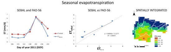
3. Results and Discussion

Figure 4 shows the seasonal cycle of daily ET obtained by the two methods used in this study. The comparison between evapotranspiration estimated by the FAO method (ETc) and SEBAL (ETSebal) shows good agreement, with an R2 = 0.87 for 2011 and R2 = 0.89 for 2012. The cumulative evapotranspiration from 16 April to 31 August, 2011 and 18 April to 9 September, 2012, as obtained by spatially integrating the ETSebal seasonal values (Figure 5), was 515 mm and 472 mm, respectively. A comparison between Figure 2 and Figure 5 shows that soil texture was generally one of the main factors controlling the ETSebal spatial distribution, with higher values found in fine soil areas. However, the spatial patterns of ET are the results of complex interactions between crops, soil texture, water table level, salinity and climate inter-annual variability. The average difference between ETc and ETSebal over the whole season was 6.4% for 2011 and 21% for 2012. This comparison is satisfactory given that the Kc coefficient method does not account for water stress factors, meaning that ETc represents an accurate estimation of ET only under well-watered conditions.
The evapotranspiration reduction coefficient Ks was used to quantify water/salinity stresses at the five monitoring stations during the 2012 growing season. Figure 6 shows daily ET for the different images calculated by SEBAL and the FAO-56 method (ETc,adj). The comparison shows a good agreement at stations B (R2 = 0.83), D (R2 = 0.78) and E (R2 = 0.85). The coefficient of determination at stations A and C were smaller (0.33 and 0.56, respectively) due to a shift in time of the ET fluxes. In station E, despite a high R2, SEBAL underestimated the ETc peak by about 30%.
Plants were affected by soil salinity stress at Stations A, C, and D. Because Station C had a very shallow water table, the daily Ks was influenced only by salt stress, while both salinity and water stress affected crop development at Stations A and D. Stations B and E were not affected by salt stress. However, severe water stress was experienced at these stations because they were both located on paleochannels in SSMU3 [36]. Consistent with other authors [51,52], SEBAL underpredicted ET with respect to the FAO dual coefficient method, even if the difference was within 20% [53]. Note that FAO-56 has been demonstrated to overestimate the actual ET values. Many authors (e.g., [54,55]) in the last 15 years have shown that the FAO-56 Kc and Kcb tabulated coefficients, even if adjusted using the specific procedure based on local meteorological, irrigation and crop data suggested by FAO-56, tend to overestimate the observed crop coefficients and actual ET in humid and semi-humid regions. Differences of up to ±40% especially during the middle growth cycle are reported in the literature, mainly due to the complexity of the crop coefficient that actually integrates several physical and biological factors [54,55]. Furthermore, other authors [56] questioned FAO-56 accuracy in estimating soil salinity effect on ET in the different growth stages.
Spatial ET dynamics calculated by SEBAL was confirmed by the 3D soil-plant model. Because of the different spatial resolution of SEBAL (30 m by 30 m) and the soil-plant model (20 m by 20 m), ordinary kriging was used to resample the 3D model results on a common 30 m by 30 m grid and compare evapotranspiration simulated by the 3D model (ETm) with ETSebal. Figure 7 shows instantaneous ET (mm/s) calculated with both models. In general, good agreement is observed between the two spatial patterns, with the lowest values in the southern sandy zone and the highest in the northern fine-texture zone. A quantitative comparison of average ET at the times of satellite overpass shows good agreement between the two methodologies with R2 = 0.70 in 2011 and R2 = 0.67 in 2012 (Figure 8). The cumulative ETm values computed by the model were in good agreement with the values provided by SEBAL.
A further model validation was performed based on the results of biomass production and maize yield. A comparison between the measured values and those simulated by the SEBAL biomass routine and the 3D soil-plant model is provided in Figure 9a for the two years. In general, the SEBAL method slightly underestimated land productivity, in contrast to the soil-plant model that overestimated yield, especially under stress conditions (2012). Measured yield data in 2011 had higher average (8.64 t/ha) and maximum (13.67 t/ha) values than in 2012 (average: 3.86 t/ha; maximum: 7.09 t/ha). SEBAL results exhibit a similar behavior, i.e., higher average (6.4 t/ha) and maximum (8.2 t/ha) values in 2011 than in the following dry year (average: 3.47 t/ha; maximum: 5.5 t/ha). Consistently, the 3D soil-plant model provided 8.69 t/ha and 11.11 t/ha for the average and maximum values in 2011, respectively, and 5.49 t/ha and 6.67 t/ha in 2012. Both methodologies are, therefore, sensitive to the observed inter-annual climate variability, but comparisons are not always satisfactory.
The yield data in 2011 and 2012 were then classified at the scale of the management units (Figure 9b,c, respectively). The results suggest that climate variability has a stronger impact on productivity than soil characteristics, differences between years being higher than those among SSMs. This is usually expected, even in areas characterized by contrasting soils [57].
The SEBAL model responded better in 2012 (average absolute error: 0.39 t/ha; average error: 10%) than in 2011 (average absolute error: 2.24 t/ha, average error: 26%), a general performance that can be evaluated as good according to [58]. It should be recalled that rainfall was spread evenly throughout the season in 2011. On the contrary, no precipitation occurred in 2012 during the early tassel and kernel blister reproductive stages, which are known to be among the most critical maize growth stages [37].
Maize yield showed high variability across the study site in both 2011 and 2012. The most productive area in both years was SSMU 4, because of the mid to low salinity and the highest clay content (Figure 10). Salinity affected maize yield in SSMU 2, which was the least productive area, while yield was intermediate in the other SSMUs.
As noted by [49], model results (both SEBAL and the 3D model) provide a good estimate of field productivity at large scales (i.e., field or SSMU) but are less effective at capturing the small-scale heterogeneities in field crop yield (Figure 11). This can be explained by a resolution problem, because both models operate on a ~10 m grid size, thus neglecting the sub-grid variability of input data (e.g., soil characteristics). However, while the 3D model is outperformed during dry conditions, due to a coarse representation of soil/root characteristics that are not required by SEBAL, this latter underestimates productivity during the wet year, probably due to the uncertainties in the utilized harvest index. In particular, even if HI may vary temporally and spatially (i.e., across the field), a single value was used here for the whole field and for both 2011 and 2012. According to the results shown in Figure 9 and published in [36], SSMU 4 was the most productive area over the 2 investigated years. This management unit may thus require a larger HI compared to the other SSMUs since it is the zone with the best conditions for maize growth. It should be noted that the HI is an important factor to estimate yield and a better knowledge on the relation between biomass production and HI will improve the accuracy of yield maps [32]. In particular, future research should clarify the impact of soil moisture conditions during flowering and crop nutrition on the harvest index [59].

4. Conclusions

In this study we used the SEBAL model in a salt-affected, water-stressed maize field in the surroundings of the Venice Lagoon, Italy, to map the spatial structure of water fluxes and crop yield. Due to the lack of measured ET data, SEBAL modeled data were not validated but only compared with ET estimates by the FAO method and three-dimensional soil-plant simulations. Nevertheless, results confirm that SEBAL is a viable tool for calculating ET at field scale even under highly heterogeneous conditions. The comparison between daily ET estimated by the FAO method and SEBAL shows good agreement in 2011 and 2012. However, in terms of crop production SEBAL responds better in 2012 (dry year) than in 2011 (wet year). SEBAL is, therefore, outperformed by a 3D soil-plant model in the case of wet conditions, but it provides far more accurate predictions in dry periods due to the fact that it does not require knowledge of the soil/root characteristics (which are crucial for soil-plant simulations, especially during drought). ET fluxes calculated at five monitoring stations installed in the area also reveal that SEBAL provides better predictions under severe water stress rather than soil salinity stress conditions.
These results suggest that the integration of SEBAL with field observations and soil-plant simulations can be very beneficial for precision agriculture practices (e.g., precision irrigation), particularly in environments where water availability is scarce or the quality of irrigation water is poor. The method presented here can be used to design and optimize variable rate irrigation strategies, thus maximizing land productivity while minimizing water losses and management costs. However, further research is needed to improve crop yield predictions at high spatial resolution in highly heterogeneous settings.

Author Contributions

F.M. and P.T. conceived and designed the experiments; C.G., G.M., M.M. performed the experiments; C.G., G.M., F.M., Y.H.C., analyzed the data; all the authors wrote the paper.

Funding

This research was supported by grants from National Commission for Space Activities (CONAE, Argentina), Córdoba National University (UNC, Argentina) and Italian Space Agency (ASI, Italy). G. Manoli acknowledges funding from the National Science Foundation (NSF-EAR-1344703).

Acknowledgments

We thank the Department of Agronomy Food Natural Resources Animals and Environment (DAFNAE), Italy and the Gulich Institute, Argentina. The authors would like to thank Elia Scudiero for conducting the field work.

Conflicts of Interest

The authors declare no conflict of interest. The funding sponsors had no role in the design of the study, in the collection, analyses, or interpretation of data, in the writing of the manuscript, nor in the decision to publish the results.

References

  1. Serageldin, I. Looking ahead: Water, life and the environment in the twenty-first century. Int. J. Water Resour. Dev. 1999, 15, 17–28. [Google Scholar] [CrossRef]
  2. Allen, R.; Tasumi, M.; Trezza, R. SEBAL (Surface Energy Balance Algorithms for Land)—Idaho Implementation—Advanced Training and Users Manual. Available online: http://www.posmet.ufv.br/wp-content/uploads/2016/09/MET-479-Waters-et-al-SEBAL.pdf (accessed on 11 September 2018).
  3. Yang, J.; Mei, X.; Huo, Z.; Yan, C.; Ju, H.; Zhao, F.; Liu, Q. Water consumption in summer maize and winter wheat cropping system based on SEBAL model in Huang-Huai-Hai Plain, China. J. Integr. Agric. 2015, 14, 2065–2076. [Google Scholar] [CrossRef]
  4. Perry, C. Accounting for water use: Terminology and implications for saving water and increasing production. Agric. Water Manag. 2011, 98, 1840–1846. [Google Scholar] [CrossRef]
  5. Burke, M.; Lobell, D.B. Satellite-based assessment of yield variation and its determinants in smallholder African systems. Proc. Natl. Acad. Sci. USA 2017, 114, 2189–2194. [Google Scholar] [CrossRef] [PubMed] [Green Version]
  6. Bastiaanssen, W.G.M.; Ali, S. A new crop yield forecasting model based on satellite measurements applied across the Indus Basin, Pakistan. Agric. Ecosyst. Environ. 2003, 94, 321–340. [Google Scholar] [CrossRef]
  7. Abtew, W.; Melesse, A. Crop Yield Estimation Using Remote Sensing and Surface Energy Flux Model. In Evaporation and Evapotranspiration: Measurements and Estimations, 1st ed.; Abtew, W., Melesse, A., Eds.; Springer: Dordrecht, The Netherlands, 2013; pp. 161–175. [Google Scholar]
  8. Molden, D.; Sakthivadivel, R. Water accounting to assess use and productivity of water. Int. J. Water Resour. Dev. 1999, 15, 55–71. [Google Scholar] [CrossRef]
  9. Burnett, B. A Procedure for Estimating Total Evapotranspiration Using Satellite-Based Vegetation Indices with Separate Estimates from Bare Soil. Master’s Thesis, University of Idaho, Moscow, ID, USA, 2007. [Google Scholar]
  10. Rwasoka, D.T.; Gumindoga, W.; Gwenzi, J. Estimation of actual evapotranspiration using the Surface Energy Balance System (SEBS) algorithm in the Upper Manyame catchment in Zimbabwe. Phys. Chem. Earth 2011, 36, 736–746. [Google Scholar] [CrossRef]
  11. Bansouleh, B.; Karimi, A.; Hesadi, H. Evaluation of SEBAL and SEBS algorithms in the estimation of maize evapotranspiration. Int. J. Plant Soil Sci. 2015, 6, 350–358. [Google Scholar] [CrossRef]
  12. Li, Y.; Zhou, Q.; Zhou, J.; Zhang, G.; Chen, C.; Wang, J. Assimilating remote sensing information into a coupled hydrology-crop growth model to estimate regional maize yield in arid regions. Ecol. Model. 2014, 291, 15–27. [Google Scholar] [CrossRef]
  13. Allen, R.G.; Pereira, L.S.; Raes, D.; Smith, M. Crop Evapotranspiration. Guidelines for Computing Crop Water Requirements; FAO Irrigation and Drainage Paper No. 56; FAO: Rome, Italy, 1998; p. 300. [Google Scholar]
  14. Morton, C.G.; Huntington, J.L.; Pohll, G.M.; Allen, R.G.; Mcgwire, K.C.; Bassett, S.D. Assessing calibration uncertainty and automation for estimating evapotranspiration from agricultural areas using METRIC. J. Am. Water Resour. Assoc. 2013, 49, 549–562. [Google Scholar] [CrossRef]
  15. Allen, R.G.; Tasumi, M.; Trezza, R. Satellite-based energy balance for mapping evapotranspiration with Internalized Calibration (METRIC)—Model. J. Irrig. Drain. Eng. 2007, 133, 380–394. [Google Scholar] [CrossRef]
  16. Anderson, M.; Gao, F.; Knipper, K.; Hain, C.; Dulaney, W.; Baldocchi, D.; Eichelmann, E.; Hemes, K.; Yang, Y.; Medellin-Azuara, J.; et al. Field-scale assessment of land and water use change over the California Delta using remote sensing. Remote Sens. 2018, 10, 889. [Google Scholar] [CrossRef]
  17. Hamada, Y.; Ssegane, H.; Negri, M.C. Mapping intra-field yield variation using high resolution satellite imagery to integrate bioenergy and environmental stewardship in an agricultural watershed. Remote Sens. 2015, 7, 9753–9768. [Google Scholar] [CrossRef]
  18. Hank, T.B.; Bach, V.; Mauser, W. Using a remote sensing-supported hydro-agroecological model for field-scale simulation of heterogeneous crop growth and yield: Application for wheat in Central Europe. Remote Sens. 2015, 7, 3934–3965. [Google Scholar] [CrossRef]
  19. Vazifedoust, M.; van Dam, J.C.; Bastiaanssen, W.G.M.; Feddes, R.A. Assimilation of satellite data into agrohydrological models to improve crop yield forecasts. Int. J. Remote Sens. 2009, 30, 2523–2545. [Google Scholar] [CrossRef]
  20. De Wit, A.; Duveiller, G.; Defourny, P. Estimating regional winter wheat yield with WOFOST through the assimilation of green area index retrieved from MODIS observations. Agric. For. Meteorol. 2012, 164, 39–52. [Google Scholar] [CrossRef]
  21. Dente, L.; Satalino, G.; Mattia, F.; Rinaldi, M. Assimilation of leaf area index derived from ASAR and MERIS data into CERES-Wheat model to map wheat yield. Remote Sens. Environ. 2008, 112, 1395–1407. [Google Scholar] [CrossRef]
  22. Bastiaanssen, W.G.M.; Menenti, M.; Feddes, R.A.; Holtslag, A.A.M. A remote sensing surface energy balance algorithm for land (SEBAL): 1. Formulation. J. Hydrol. 1998, 212–213, 198–212. [Google Scholar] [CrossRef]
  23. Elhaddad, A.; Garcia, L. Surface Energy Balance-Based Model for Estimating Evapotranspiration Taking into Account Spatial Variability in Weather. J. Irrig. Drain. Eng. 2008, 134, 681–689. [Google Scholar] [CrossRef]
  24. Suleiman, A.A.; Bali, K.M.; Kleissl, J. Comparison of ALARM and SEBAL evapotranspiration of irrigated alfalfa. In Proceedings of the 2009 ASABE Annual International Meeting, Grand Sierra Resort and Casino, Reno, NV, USA, 21–24 June 2009; pp. 2318–2325. [Google Scholar] [CrossRef]
  25. Chávez, J.; Neale, C.M.U.; Hipps, L.E.; Prueger, J.H.; Kustas, W.P. Comparing aircraft-based remotely sensed energy balance fluxes with eddy covariance tower data using heat flux source area functions. J. Hydrometeorol. 2005, 6, 923–940. [Google Scholar] [CrossRef]
  26. Gowda, P.H.; Howell, T.A.; Paul, G.; Colaizzi, P.D.; Marek, T.H. Sebal for Estimating Hourly ET Fluxes over Irrigated and Dryland Cotton during BEAREX08; World Environmental and Water Resources Congress: Reston, VA, USA, 2011; pp. 2787–2795. [Google Scholar]
  27. Bastiaanssen, W.G.M.; Noordman, E.M.; Davids, G.; Thoreson, B.P.; Allen, R.G. SEBAL model with remotely sensed data to improve water-resources management under actual field conditions. J. Irrig. Drain. Eng. 2005, 131, 85–93. [Google Scholar] [CrossRef]
  28. Singh, R.K.; Irmak, A.; Irmak, S.; Martin, D.L. Application of SEBAL model for mapping evapotranspiration and estimating surface energy fluxes in South-Central Nebraska. J. Irrig. Drain. Eng. 2008, 134, 273–285. [Google Scholar] [CrossRef]
  29. De Teixeira, A.H.C.; Bastiaanssen, W.G.M.; Ahmad, M.D.; Bos, M.G. Reviewing SEBAL input parameters for assessing evapotranspiration and water productivity for the Low-Middle Sao Francisco River basin, Brazil. Part A: Calibration and validation. Agric. For. Meteorol. 2009, 149, 462–476. [Google Scholar] [CrossRef] [Green Version]
  30. Tang, R.; Li, Z.L.; Chen, K.; Jia, Y.; Li, C.; Sun, X. Spatial-scale effect on the SEBAL model for evapotranspiration estimation using remote sensing data. Agric. For. Meteorol. 2013, 174–175, 28–42. [Google Scholar] [CrossRef]
  31. Scott, C.A.; Bastiaanssen, W.G.M.; Ahmad, M.D. Mapping root zone soil moisture using remotely sensed optical imagery. J. Irrig. Drain. Eng. 2003, 129, 326–335. [Google Scholar] [CrossRef]
  32. Zwart, S.J.; Bastiaanssen, W.G.M. SEBAL for detecting spatial variation of water productivity and scope for improvement in eight irrigated wheat systems. Agric. Water Manag. 2007, 89, 287–296. [Google Scholar] [CrossRef]
  33. Bastiaanssen, W.; Thoreson, B.; Byron, C.; Davids, G. Discussion of “Application of SEBAL Model for Mapping Evapotranspiration and Estimating Surface Energy Fluxes in South-Central Nebraska” by Ramesh K. Singh, Ayse Irmak, Suat Irmak, and Derrel L. Martin. J. Irrig. Drain. Eng. 2010, 136, 282–283. [Google Scholar] [CrossRef]
  34. Scudiero, E.; Deiana, R.; Teatini, P.; Cassiani, G.; Morari, F. Constrained optimization of spatial sampling in salt contaminated coastal farmland using EMI and continuous simulated annealing. Procedia Environ. Sci. 2011, 7, 234–239. [Google Scholar] [CrossRef]
  35. Scudiero, E.; Teatini, P.; Corwin, D.L.; Deiana, R.; Berti, A.; Morari, F. Delineation of site-specific management units in a saline region at the Venice Lagoon margin, Italy, using soil reflectance and apparent electrical conductivity. Comput. Electron. Agric. 2013, 99, 54–64. [Google Scholar] [CrossRef]
  36. Scudiero, E.; Teatini, P.; Corwin, D.L.; Dal Ferro, N.; Simonetti, G.; Morari, F. Spatio-temporal response of maize yield to edaphic and meteorological conditions in a saline farmland. Agron. J. 2014, 106, 2163–2174. [Google Scholar] [CrossRef]
  37. Manoli, G.; Bonetti, S.; Domec, J.C.; Putti, M.; Katul, G.; Marani, M. Tree root systems competing for soil moisture in a 3D soil-plant model. Adv. Water Resour. 2014, 66, 32–42. [Google Scholar] [CrossRef]
  38. Scudiero, E.; Berti, A.; Teatini, P.; Morari, F. Simultaneous monitoring of soil water content and salinity with a low-cost capacitance-resistance probe. Sensors 2012, 12, 17588–17607. [Google Scholar] [CrossRef] [PubMed]
  39. Tasumi, M.; Allen, R.G.; Trezza, R. At-surface albedo from Landsat and MODIS satellites for use in energy balance studies of evapotrans-piration. J. Hydrol. Eng. 2008, 13, 51–63. [Google Scholar] [CrossRef]
  40. Tasumi, M.; Trezza, R.; Allen, R.G.; Wright, J.L. US Validation tests on the SEBAL model for evapotranspiration via satellite. In Proceedings of the 54th IEC Meeting of the International Commission on Irrigation and Drainage (ICID), Workshop Remote Sensing of ET for Large Regions, Montpellier, France, 14–19 September 2003. [Google Scholar]
  41. Markham, B.L.; Barker, J.L. Landsat MSS and TM Post-Calibration Dynamic Ranges, Exoatmospheric Reflectances and At-Satellite Temperatures; EOSAT Landsat Technical Notes 1:3-8; Earth Observation Satellite Company: Lanham, MD, USA, 1986. [Google Scholar]
  42. Alexandridis, T.K.; Cherif, I.; Chemin, Y.; Silleos, G.N.; Stavrinos, E.; Zalidis, G.C. Integrated methodology for estimating water use in mediterranean agricultural areas. Remote Sens. 2009, 1, 445–465. [Google Scholar] [CrossRef]
  43. Schaap, M.G.; Leij, F.J.; Van Genuchten, M.T. Rosetta: A computer program for estimating soil hydraulic parameters with hierarchical pedotransfer functions. J. Hydrol. 2001, 251, 163–176. [Google Scholar] [CrossRef]
  44. GRASS Development Team. GRASS GIS v7 Download. Available online: http://grass.itc.it/download/index.php (accessed on 9 July 2009).
  45. Brutsaert, W.; Sugita, M. Application of self-preservation in the diurnal evolution of the surface energy budget to determine daily evaporation. J. Geophys. Res. 1992, 97, 377–382. [Google Scholar] [CrossRef]
  46. Chemin, Y.; Alexandridis, T. Improving spatial resolution of et seasonal for irrigated rice in Zhanghe, China. In Proceedings of the 22nd Asian Conference on Remote Sensing, Singapore, 5–9 November 2011. [Google Scholar]
  47. Chemin, Y.; Platonov, A.; Abdullaev, I.; Ul-Hassan, M. Supplementing farm-level water productivity assessment by remote sensing in transition economies. Water Int. 2005, 30, 513–521. [Google Scholar] [CrossRef]
  48. Giardini, L.; Berti, A.; Morari, F. Simulation of two cropping systems with EPIC and CropSyst models. Ital. J. Agron. 1998, 1–2, 29–38. [Google Scholar]
  49. Manoli, G.; Bonetti, S.; Scudiero, E.; Morari, F.; Putti, M.; Teatini, P. Modeling soil—Plant dynamics: Assessing simulation accuracy by comparison with spatially distributed crop yield measurements. Vadose Zone J. 2015, 14. [Google Scholar] [CrossRef]
  50. Katul, G.; Manzoni, S.; Palmroth, S.; Oren, R. A stomatal optimization theory to describe the effects of atmospheric CO2 on leaf photosynthesis and transpiration. Ann Bot. 2010, 105, 431–442. [Google Scholar] [CrossRef] [PubMed]
  51. Ramos, J.G.; Cratchley, C.R.; Kay, J.A.; Casterad, M.A.; Martínez-Cob, A.; Domínguez, R. Evaluation of satellite evapotranspiration estimates using ground-meteorological data available for the Flumen District into the Ebro Valley of N.E. Spain. Agric. Water Manag. 2009, 96, 638–652. [Google Scholar] [CrossRef] [Green Version]
  52. Kite, G.W.; Droogers, P. Comparing evapotranspiration estimates from satellites, hydrological models and field data. J. Hydrol. 2000, 229, 3–18. [Google Scholar] [CrossRef]
  53. Allen, R.G. Using the FAO-56 dual crop coefficient method over an irrigated region as part of an evapotranspiration intercomparison study. J. Hydrol. 2000, 229, 27–41. [Google Scholar] [CrossRef]
  54. Katerji, N.; Rana, G. Modelling evapotranspiration of six irrigated crops under Mediterranean climate conditions. Agric. Meteorol. 2006, 138, 142–155. [Google Scholar] [CrossRef]
  55. Facchi, A.; Gharsallah, O.; Gandolfi, C. Evapotranspiration models for a maize agro-ecosystem in irrigated and rainfed conditions. J. Agric. Eng. 2013, 44. [Google Scholar] [CrossRef] [Green Version]
  56. Abedinpour, M.; Sarangi, A.; Rajput, T.B.S.; Singh, M.; Pathak, H.; Ahmad, T. Performance evaluation of AquaCrop model for maize crop in a semi-arid environment. Agric. Water Manag. 2012, 110, 55–66. [Google Scholar] [CrossRef]
  57. McBratney, A.B.; Minasny, B.; Whelan, B.M. Obtaining ‘useful’ high-resolution soil data from proximally sensed electrical conductivity/resistivity (PSEC/R) surveys. Precis. Agric. 2005, 5, 503–510. [Google Scholar]
  58. Cannavo, P.; Recous, S.; Parnaudeau, V.; Reau, R. Modeling N dynamics to assess environmental impacts of cropped soils. Adv. Agron. 2008, 97, 131–174. [Google Scholar] [CrossRef]
  59. Bastiaanssen, W.G.M.; Steduto, P. The water productivity score (WPS) at global and regional level: Methodology and first results from remote sensing measurements of wheat, rice and maize. Sci. Total Environ. 2017, 575, 595–611. [Google Scholar] [CrossRef] [PubMed]
Figure 1. The study area: (a) aerial image of the study area at the southern edge of the Venice Lagoon, Italy; (b) delineation of site-specific management units (SSMUs) based on [35] and monitoring stations (A, B, C, D, E).
Remotesensing 10 01452 g001
Figure 2. Site characterization: (a) land and (b) water table elevation [m above sea level, masl], average (c) soil texture (as sand percentage [%]), and (d) soil salinity (in terms of ECe [dS m−1]) in the 0–1.2 m soil profile.
Remotesensing 10 01452 g002
Figure 3. Boxplots for (a) EC1:2, electrical conductivity of a soil extract with a soil to water ratio of 1:2, (b) soil bulk density, (c) soil organic carbon content, and (d) clay content.
Remotesensing 10 01452 g003
Figure 4. Temporal variation of evapotranspiration (ET) (mm/day) computed by surface energy balance algorithm for land (SEBAL) and Food and Agriculture Organization (FAO-56) approaches from April to September: (a) 2011, (b) 2012. ETSebal versus ETc results: (c) 2011 and (d) 2012. Dotted lines represent the identity line (1:1).
Remotesensing 10 01452 g004
Figure 5. Map of seasonal evapotranspiration (ETs) (mm) for the study site in 2011 (16 April–31 August) and 2012 (18 April–9 September) as obtained by Equation (6). SSMUs are overlaid (white lines and numbers).
Remotesensing 10 01452 g005
Figure 6. Temporal variation of ETSebal and ETc,adj (mm/day) at the five monitoring stations: (a) Station A, (b) Station B, (c) Station C, (d) Station D, (e) Station E. ETSebal versus ETc,adj: (f) Station A, (g) Station B, (h) Station C, (i) Station D, (j) Station E.
Remotesensing 10 01452 g006
Figure 7. Detailed map of instantaneous ET (mm/s) distribution at the study site as predicted by SEBAL and the soil-plant model: (a) ETSebal Day of Year (DOY) 138 2011; (b) ETSebal DOY 157 2012; (c) ETm DOY 138 2011; (d) ETm DOY 157 2012.
Remotesensing 10 01452 g007
Figure 8. Temporal variation of instantaneous ET (mm/s) calculated with SEBAL and the 3D soil-plant model: (a) 2011, (b) 2012. Instantaneous ET from SEBAL versus that from the 3D soil-plant model: (c) 2011, (d) 2012.
Remotesensing 10 01452 g008
Figure 9. (a) Measured and computed average yield in 2011 and 2012. Measured and computed average yield in the SSMUs in (b) 2011 and (c) 2012.
Remotesensing 10 01452 g009
Figure 10. Maps of maize yield (t/ha) in the study area: (ac): 2011 measured yield, SEBAL yield, and 3D soil-plant model yield, respectively; (df): 2012 measured yield, SEBAL yield, and 3D soil-plant model yield, respectively.
Remotesensing 10 01452 g010
Figure 11. Yield maps: absolute and relative errors in 2011 (a,b) and 2012 (c,d) using the SEBAL model.
Remotesensing 10 01452 g011

