Realistic Forest Stand Reconstruction from Terrestrial LiDAR for Radiative Transfer Modelling

Abstract

Forest biophysical variables derived from remote sensing observations are vital for climate research. The combination of structurally and radiometrically accurate 3D “virtual” forests with radiative transfer (RT) models creates a powerful tool to facilitate the calibration and validation of remote sensing data and derived biophysical products by helping us understand the assumptions made in data processing algorithms. We present a workflow that uses highly detailed 3D terrestrial laser scanning (TLS) data to generate virtual forests for RT model simulations. Our approach to forest stand reconstruction from a co-registered point cloud is unique as it models each tree individually. Our approach follows three steps: (1) tree segmentation; (2) tree structure modelling and (3) leaf addition. To demonstrate this approach, we present the measurement and construction of a one hectare model of the deciduous forest in Wytham Woods (Oxford, UK). The model contains 559 individual trees. We matched the TLS data with traditional census data to determine the species of each individual tree and allocate species-specific radiometric properties. Our modelling framework is generic, highly transferable and adjustable to data collected with other TLS instruments and different ecosystems. The Wytham Woods virtual forest is made publicly available through an online repository.

1. Introduction

Climate research is underpinned by the provision of remote sensing data, which provides global coverage and regular repeat cycles. Essential Climate Variables (ECVs), such as leaf area index (LAI) and fraction of absorbed photosynthetically active radiation (fAPAR), are routinely derived from these data across scales from 10 s of metres to kilometres, and assist in the evaluation of the response of vegetation to climate change. A wide range of indirect methods and instruments have been developed for the in situ measurement of LAI and fAPAR but the understanding of their associated uncertainties, assumptions and how they relate to large scale remote sensing data is limited [1,2]. The same applies for the development and testing of essential biodiversity variables (EBVs), which are increasingly important to estimate and to predict the performance of ecosystems. Providing interoperability for in situ and large scale remote sensing data is challenging without having a common reference. Without well-quantified uncertainty, interoperability (the comparison between and within datasets) is not recommended and thus confidence in the use of such data is severely limited. Radiative transfer (RT) models provide a critical link between the 3D measurement and model representations of forests (“virtual” forests) and the resulting simulated remote sensing signal [3,4]. This link between forest structure and the radiometric signal allows the inversion of biophysical properties from remote sensing measurements. RT models allow us to calculate and control all aspects of the forest structure and the simulated signal, meaning that testing of various assumptions is possible. This allows for the simulation of any sensor and observation configuration, retrieval of biophysical properties with quantified uncertainty, as well as providing a framework for quantifying end-to-end traceability. This is key for parameter retrieval, as well as product comparison and validation and will help international initiatives and programmes such as the GEO-BON Working Group, the CEOS Working Group on Calibration and Validation (WGCV) and the European Copernicus Climate Change Service (C3S) with provision of quantified climate analysis ready datasets.

Virtual 3D models generally consist of a structural and a radiometric component. Widlowski et al. [3] gives a comprehensive overview of radiometric properties in RT vegetation simulations. The structural component of 3D models varies widely. Virtual forest stands can be seen as a collection of individual trees, as a voxel representation or somewhere in between. Individual tree structure can be represented through crown archetypes (e.g., conical, ellipsoidal) or geometrically explicit 3D models of all canopy elements (i.e., individual leaves, branches and stem). Crown archetypes typically do not account for within-crown clumping and care is needed in inferring biophysical properties from these abstract representations [5,6,7]. Geometrically explicit 3D models generally make fewer assumptions, but are initially a lot more labour intensive to generate. This often involved a manual procedure to match measured field data with modelling parameters used in 3D model generating software. Widlowski et al. [3] used different virtual forests for the fourth phase of the radiative transfer model intercomparison (RAMI-IV). These models consisted of individual trees that were generated with the xfrog [8] or arbaro [9] software based on field inventory data or tree crown information extracted from airborne LiDAR. The geometry of individual leaves was modelled on the basis of information obtainable from the internet [3]. Other studies used OnyxTree (www.onyxtree.com) software [10,11] to generate geometrically explicit tree models based on parameters measured in the field and parametric modelling of plant anatomy, topology, and growth. Terrestrial laser scanning (TLS, also called terrestrial LiDAR) [12] enabled fast and automated modelling of explicit 3D branching structure of trees [13,14,15]. Côté et al. [16,17] introduced the L-Architect model to reconstruct structural and radiative consistent conifer models. L-Architect extracts the woody-returns from the full LiDAR point cloud to create the branching structure and adds foliage based on light availability derived from the point cloud. Åkerblom et al. [18] introduced an algorithm to insert needleleaves or broadleaves to geometric 3D models. However, the addition of foliage remains challenging due to self-occlusion effects in TLS data. Generally, only a limited number of trees have been explicitly modelled to build up a tree library. Virtual stands can then be generated using a look-up table approach combined with a random azimuthal rotation for each individual tree [3,10,19].

Here, we present a semi-automated framework for creating virtual forests from terrestrial LiDAR. Our approach uses a unique leaf-off/leaf-on dataset and open source software. We explicitly model every tree in the scene, and therefore reduce assumptions compared to models that use a limited tree library. Such realistic virtual forests models are of great value for testing algorithms and providing a better understanding of the interaction between the derived parameters and the forest structure. They are essentially the only way to do realistic calibration and validation at the scales of earth observation (EO) data (e.g., 20–30 m and wider), as well as to provide useful uncertainty assessment. The virtual forest stand generated within this paper represents a one hectare stand of deciduous forest in Wytham Woods (UK) and is made publicly available (see Section 5) together with the open-source methods. We see the role of TLS-derived accurate 3D virtual forest models being increasingly useful for underpinning large-scale EO biophysical product development.

2. Materials and Methods

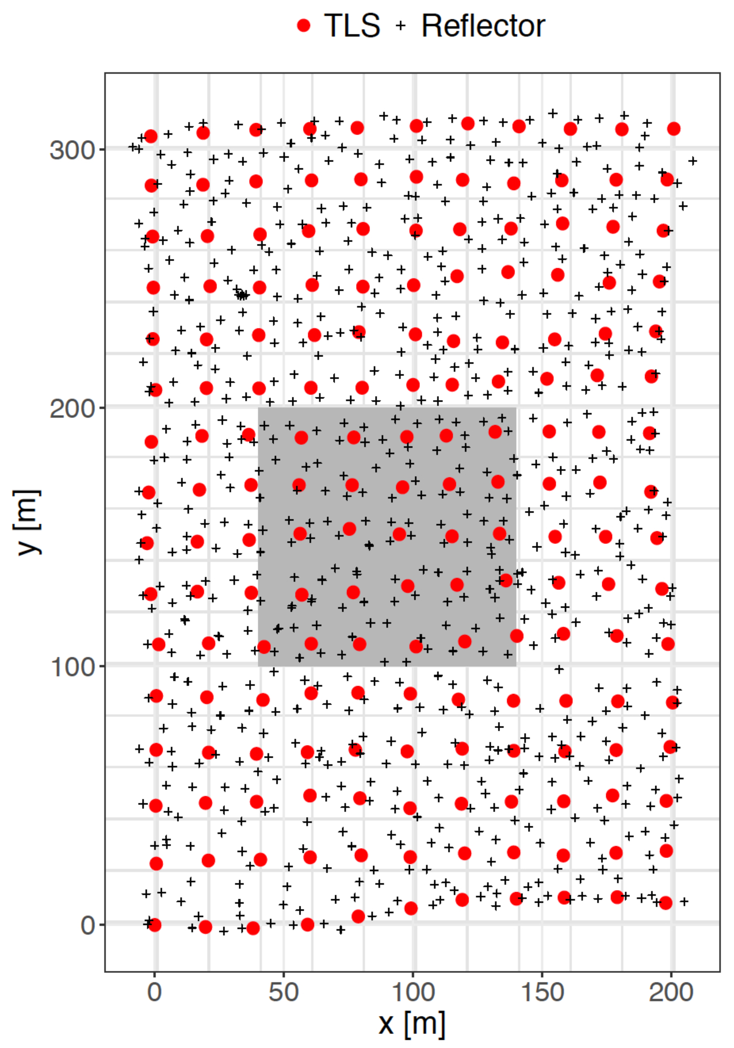
2.1. Study Area and Data Collection

A six-hectare study site (200 × 300 m) was established in Wytham Woods, UK. The site is nested within an 18 hectare long-term forest inventory plot that is run by Oxford University and is part of the ForestGEO global network of forest inventory plots. The forest is dominated by Acer pseudoplatanus (Sycamore), Fraxinus excelsior (Ash) and Corylus avellana (Hazel). The mean annual temperature is 10 ${}^{\circ }$C, the mean annual rainfall is 726 mm and the mean annual radiation is 118 W/m${}^2$ [20]. Based on the forest inventory census, the average diameter at breast height (DBH) is 35.2 cm and the median DBH is 24 cm. The smallest DBH in the census is 2.9 cm and the largest DBH is 141.2 cm. Structural 3D data were collected with a RIEGL VZ-400 terrestrial laser scanner (RIEGL Laser Measurement Systems GmbH), which uses on-board waveform processing. This instrument records multiple return LiDAR data, which improves vertical sampling [21,22]. TLS data were collected in leaf-on (June & July 2015) and leaf-off (December 2015 & January 2016) conditions (Figure 1).

The wavelength of the instrument is 1550 nm and the beam divergence is nominally 0.35 mrad. The angular sampling for both zenith and azimuth angle is 0.04${}^{\circ }$, azimuth range is 0${}^{\circ }$–360${}^{\circ }$ and zenith range is 0${}^{\circ }$–130${}^{\circ }$. The complete six hectares were scanned from 176 scan locations, laid out in a 20 × 20 m regular grid [23]. Reflective targets were used to co-register all the scan locations to a single point cloud using RIEGL’s RiSCAN PRO software package [24]. For the forest stand reconstruction, we focussed on a one hectare subset of the registered point cloud only: the 100 × 100 m subset with SW-coordinate (40, 100) and NE-coordinate (140, 200) (Figure A1). The local origin coordinate (0,0) was measured with a differential GPS and located at Lat 51.7750579, Lon-1.33904729. This ensured the highest quality TLS data since, as Wilkes et al. [24] point out, scan locations from outside the modelled plot provide essential LiDAR returns and reduce occlusions near the border of the plot (especially near the top of the trees). The nearest neighbourhood analysis of the average distance to the four nearest neighbours (Figure A2) shows that occlusion in leaf-on TLS data is larger than leaf-off TLS data.

2.2. Forest Stand Reconstruction

Forest stand reconstruction from a co-registered point cloud requires three main steps: (1) tree segmentation; (2) tree structure modelling and (3) leaf addition. We made use of existing open-source software for each step (see

Table 1. Open-source software used for forest stand reconstruction.

Processing Step	Automation	Reference	Link
(1) Tree Extraction	Semi-Automated	[25], Burt [26]	github.com/apburt/treeseg
(2) Tree structure Modelling	Automated	Raumonen et al. [13], Calders et al. [15]	github.com/InverseTampere/TreeQSM
(3) Leaf Addition	Automated	Åkerblom et al. [18]	github.com/InverseTampere/qsm-fanni-matlab

). We used the leaf-off TLS data for the tree extraction and modelling of the forest stand structure (steps 1 and 2). Leaf-on and leaf-off data were used in the final leaf addition step.

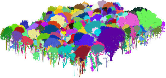
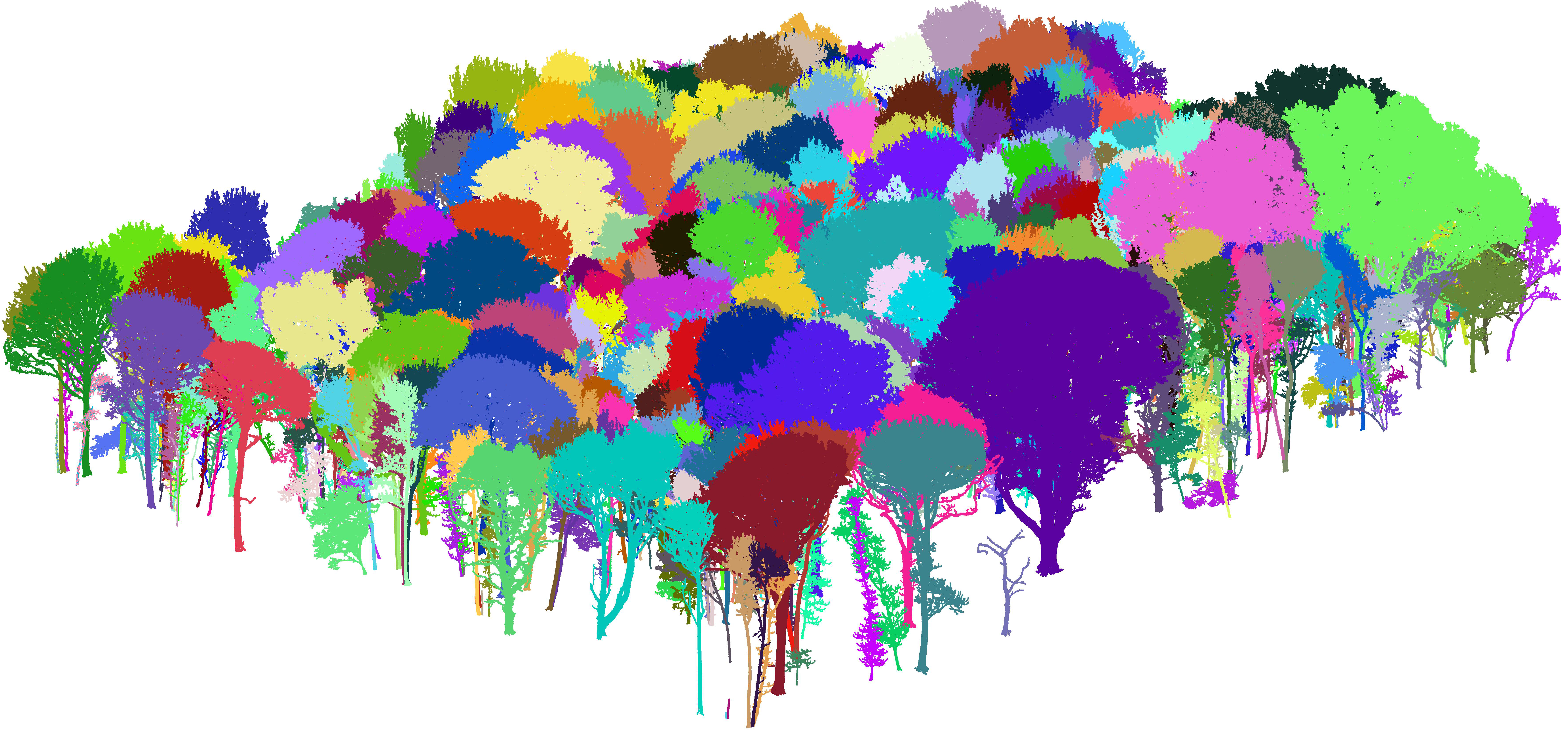
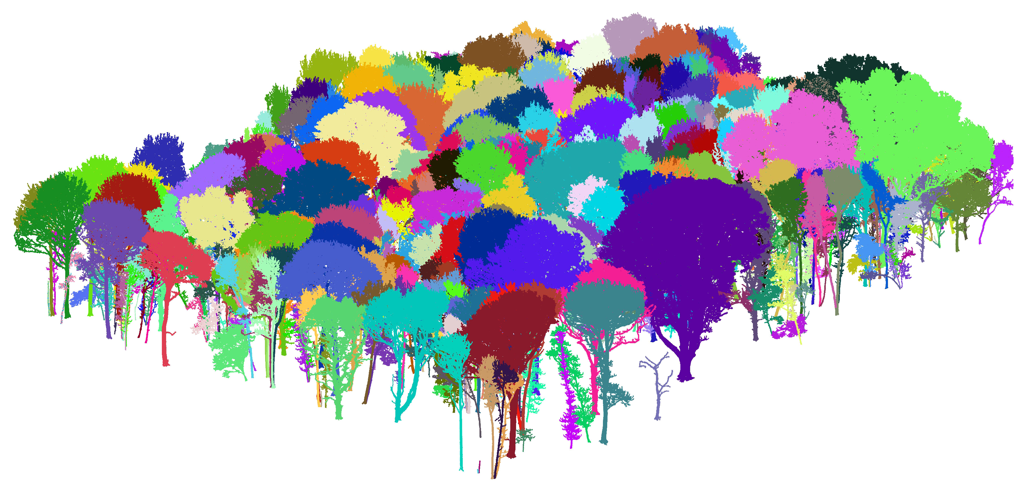
2.2.1. Tree Extraction

The first step extracted single trees from the registered point cloud. If a multi-stem tree splits below 1.3 m, each stem was considered to be an individual tree. Tree segmentation used the treeseg open-source software. This software built upon the Point Cloud Library [27]. It uses few a priori assumptions about tree architecture and is mainly data-driven. This method utilises generic point cloud processing techniques including Euclidean clustering, principal component analysis, region-based segmentation, shape fitting and connectivity testing. Full details of this method can be found in [25]. The following steps were followed to segment the leaf-off point cloud:

• Filtering. Spurious points were detected and removed. We used the deviation of the recorded waveform with the stored reference waveforms’ shapes to define the quality of a point in the point cloud [28].
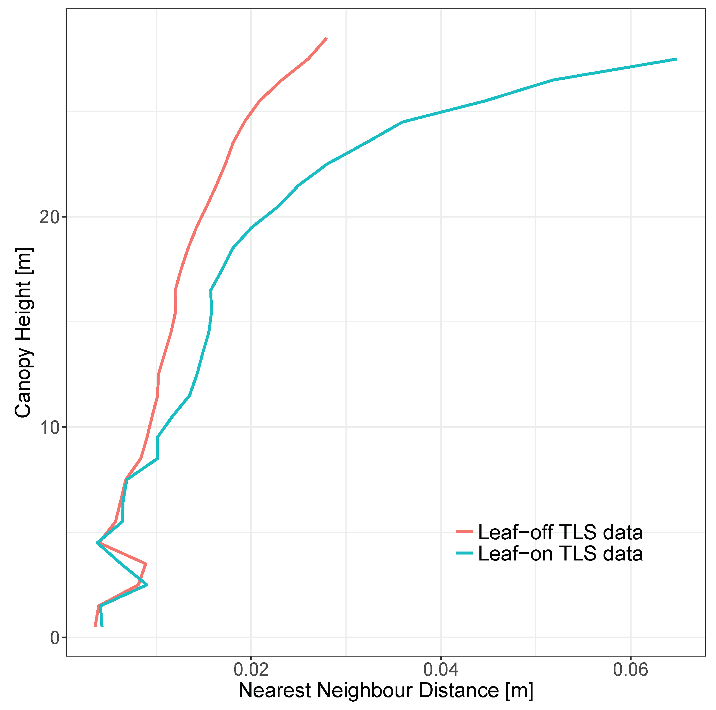
• Downsampling. Many processing steps are susceptible to the variation in nearest neighbour distance. It is therefore recommended [25] to downsample the point cloud via voxel grid aggregation. We downsampled the original point cloud to 0.026 m resolution. This resolution was decided based on the analysis of the 4 nearest neighbours for each point and the consideration of the beam exit diameter, beam divergence and approximate path length through the canopy.
• Stem Identification & Stem Segmentation. We identified individual stems through segmentation of a height slice above the ground plane. This required the following steps: (a) A DTM was constructed across the larger-area point cloud, from which a slice in the point cloud, in the z-axis, was generated. We used a 2 m slice between 1 and 3 m above the terrain (1 m DTM); (b) This slice was organised into sets of point clouds representing common underlying surfaces via Euclidean clustering and region-based segmentation and (c) each set was considered a stem based on the residual error of multiple RANSAC cylinder fits, and the angle between the vector of the cylinder centreline and the vector perpendicular to the underlying DTM tile plane.
• Crown Isolation. Sequential identification of point clusters defined by point density in height slices along the length of the tree to remove unrelated vegetation and noise from these clouds.
• Visual Inspection. Quality control and, if necessary, removing or adding crown material. This will happen most likely in trees with overlapping crowns and in smaller understorey shrubs.

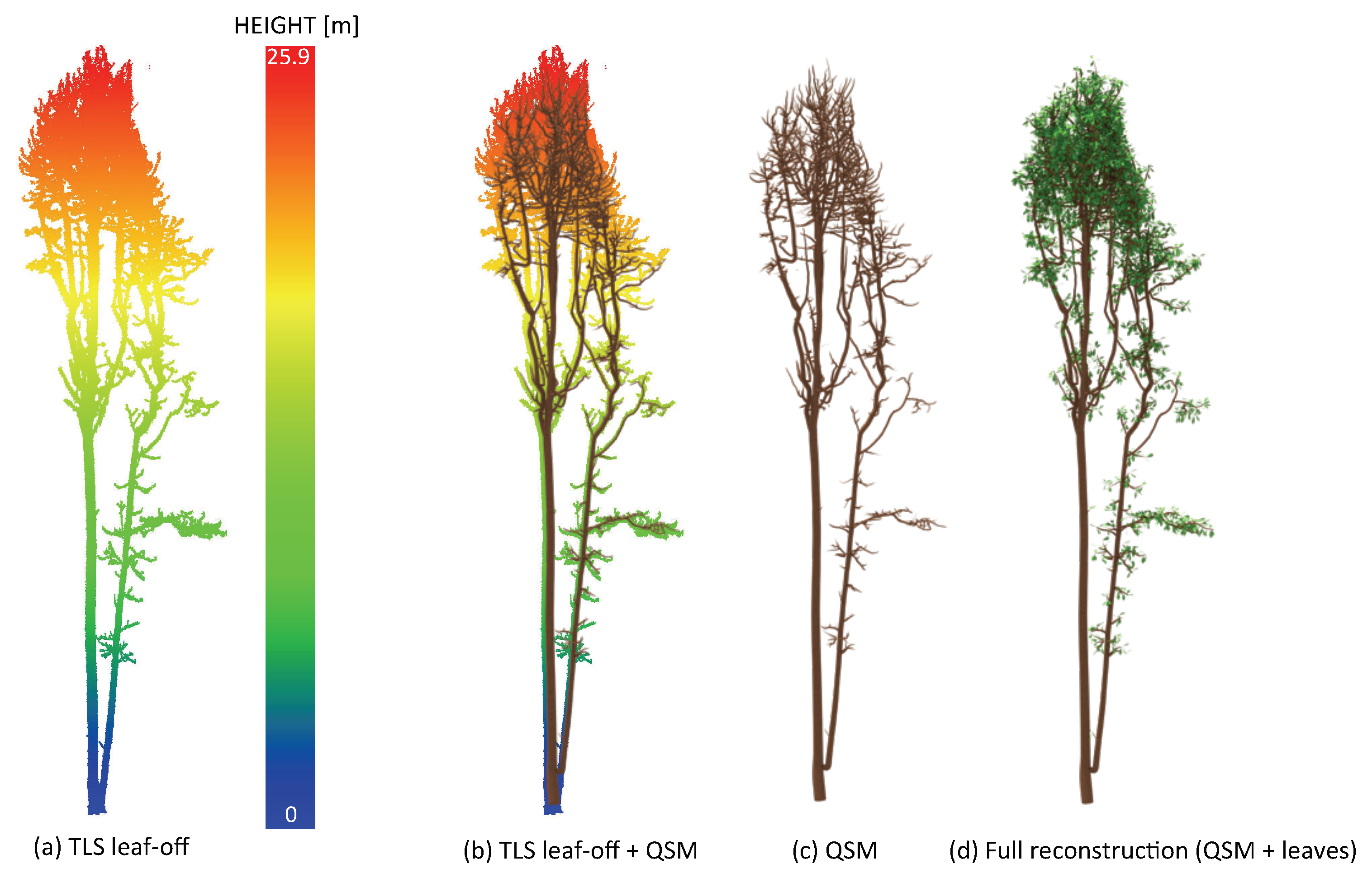
2.2.2. Tree Structure Modelling

In this step, individual tree leaf-off point clouds were converted to Quantitative Structure Models (QSMs) [14,29]. We used the QSM workflow described in [15]. This approach builds on Raumonen et al. [13] and fits cylinders to the point cloud data following the skeleton of the tree point cloud. Åkerblom et al. [30] compared various geometric primitives and found that the cylinder is the most robust primitive in the sense of a well-bounded volumetric modelling error, particularly with noise and gaps in the data.

The most important input parameter for the QSM method is the cover patch size (d), which essentially defines the size of the point cloud building blocks to reconstruct the tree from the base up. Volumetric estimation from QSMs can vary significantly depending on the choice of d [15,31], so getting d “right” is critical: if d is too small, the modelled cylinders will tend to enclose a smaller volume than they ought to; if d is too large, the modelled cylinders will tend to fit volumes that are too large to the point cloud. Calders et al. [32] described an automated framework for autonomous optimisation of cover patch size d and demonstrated that volume estimates from automated QSM parameter setting agreed with those values derived from visual assessment. The uncertainties at tree level can be higher for the automated QSM assessment, but the stand level volume agreed to within 6.8% with the reference data. Here, we used a modified version, with parameters optimised for this particular ecosystem structure:

• The single tree point cloud was reconstructed 10 times over the desired d-range of 0.02 m to 0.11 m at an increment of 0.005 m.
• For each of the 10 QSMs for each d value, 4 trunk cylinders at 7.5%, 10%, 12.5% and 15% of the trunk length were extracted from the QSMs. The coordinates of these four cylinders drive a pass-through filter to extract the point cloud slice from which the QSM was formed.
• The trunk diameters were estimated using least squares circle fitting on the point cloud slices and the diameters compared with the cylinders as a percentage change to quantify model conformity to the cloud. A single value (trunk${}_{match}$) is calculated by averaging the four diameter comparisons for each of the 10 models.
• For each d value the mean and standard deviation were generated from the 10 models. The coefficients of variation (CVs) are calculated as standard deviation/mean.
• The lowest d value that conforms to (CV < CV${}_{threshold}$) and (trunk${}_{match}$ > trunk${}_{conformity}$) was selected as the optimised d. We used CV${}_{threshold}$ = 5 × CV${}_{min}$ (see [26]) and trunk${}_{conformity}$ = 0.95. CV${}_{min}$ is the minimum CV. Trunk${}_{conformity}$ can be modified for forests where trees often have irregular forms (e.g., presence of buttressed trunks [33]).
• If no optimised d is identified in step five, the method falls back onto the d with the lowest CV.

After the optimised d has been determined, a single iteration for that d value was chosen randomly to represent the woody architecture in our 3D model.

2.2.3. Leaf Addition

Leaves were added to the tree QSM structure using the Foliage and Needles Naïve Insertion (FaNNI) algorithm described in Åkerblom et al. [18]. This algorithm allows for controlling distributions of leaf location, size and angles and the shape of individual leaves, allowing users to fine-tune these parameters for a specific tree or forest stand. Within this paper we used the following parameters and distributions:

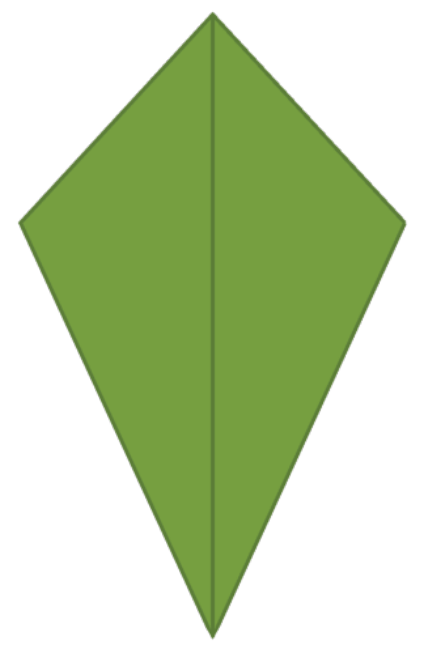
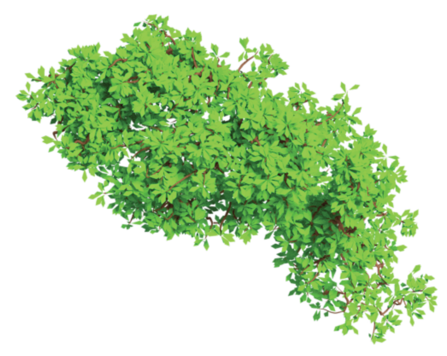
• Leaf shape: tetragon (see Figure 2).
• Target leaf area.
• Leaf area density distribution (LADD): the probability of a cylinder to have leaves depended on its relative height along the tree, the cylinders position along the respective branch and the order of that branch. Height-dependent leaf area probability was interpolated linearly from 0.2 at ground level to 1.0 at tree top. Leaves are allowed to occupy the last 5% of the stem, with that percentage rising with the branch order, reaching 60% for branch orders four and up. For more details see the definition of LADD 2 in Åkerblom et al. [18].
• Leaf size distribution (LSD): a uniform distribution where the length of the tetragon is sampled between 25 cm and 30 cm. This length was selected as a trade-off between the number of objects (i.e., leaves) and RAM requirements.
• Leaf orientation distribution (LOD): an initial leaf normal is generated depending on the generated petiole directions. If the initial normal is less than 20${}^{\circ }$ different compared to a reference vector pointing straight up, then the final normal points straight up. Otherwise the initial normal is rotated 20${}^{\circ }$ towards the reference vector and used as the final normal, resulting in most leaves facing upwards but with some random variation. For more details see the definition of the default leaf orientation distribution in Åkerblom et al. [18].

The algorithm is given a starting leaf area (equal to 1.3× target leaf area), allowing intersecting leaf-candidates to be discarded if necessary. The target leaf area was determined from analysis of the 176 leaf-on and leaf-off scans of the six hectares study area. Gap fraction analysis allowed us to calculate the average effective wood area index (eWAI, leaf-off) and effective plant area index (ePAI, leaf-on) using the approach detailed in [34,35] and a detailed description of the ePAI and eWAI analysis of Wytham Woods is described in Calders et al. [2]. Calders et al. [2] suggested a linear regression model to estimate eLAI from ePAI - eWAI (eLAI = 0.552 + 1.069 × (ePAI-eWAI), $R^2$ = 0.87) based on radiative transfer simulations of eWAI, ePAI and eLAI for a deciduous stand resembling the forest structure of Wytham Woods. Here, we have assumed a clumping index $\mathrm{\Omega }$ of 0.98 [36] and the total leaf area for our one hectare model was calculated as 10,000× eLAI/$\mathrm{\Omega }$. The target leaf area per tree was calculated by distributing the total model leaf area based on the relative tree branch length. Tree branch length was calculated using the QSMs of the tree structure.

2.2.4. Radiometric Properties

Field measurements using a FieldSpec (ASD Spectrometer) were collected to provide the spectral characteristics of the leaves, bark and understorey (in summer and winter). Understorey reflectance measurements were taken with the ASD Spectrometer using the pistol (bare fibre). Measurements were taken at a height of 1 m with the operator facing north. One measurement, formed from the average of five samples, was taken in the middle of each 20 × 20 m grid. A white reference panel measurement was taken every five measurements. Additional white reference measurements were taken during changeable solar and atmospheric conditions. Spectral measurements of leaves were taken using the ASD leaf clip and plant probe attached to the ASD Spectrometer. Twenty-seven trees were selected from the Wytham Woods census based on the number of trees of each species present. For each of the 27 selected trees, two branches were cut and five leaves per branch were sampled. Branches were cut from trees and sampled within approximately 20 minutes. Spectral measurements of the bark for the 27 selected trees were taken using the ASD contact probe attached to the ASD Spectrometer.

The TLS stem map was linked with the inventory census to determine the species for each tree. Each species was then linked to the appropriate radiometric properties.

2.3. Radiative Transfer Modelling

The librat Monte Carlo Ray Tracing (MCRT) model, a library of C functions, was used in this project. It is based on the ararat/drat MCRT model [37]. Ray tracing involves firing photons into the scene and analysing its behaviour each time it intersects a scene element. At the intersections, diffuse ray paths are also generated, which will contribute to multiple scattering. These rays can be terminated either after a certain threshold value is achieved or by escaping out of the scene. Radiometric properties (i.e., reflection, absorption and transmission) are used to quantify the attenuation along its trajectory. Selection of the photon trajectories and convergence towards a steady solution in ray tracing is achieved via the Monte Carlo method. Librat has been tested in earlier studies, as well as against other models [38,39] and observations [5,40].

The RT model of Wytham Woods is stored in ASCII .obj geometry definition files. This is a modified version of the open Wavefront format (https://www.fileformat.info/format/wavefrontobj/egff.htm). The scene is represented using a hierarchy of .obj files, with the scene at the top level, including individual tree files and their locations, with each tree including the structure as well as their associated radiometric properties. For each tree, the leaves and branching architecture were stored in separate obj-files. The background digital terrain model (DTM, 1 m resolution) represented the terrain as well as the understorey reflectance. The DTM was created through Delaunay triangulation of the lowest point detected in a one metre area in the leaf-off TLS data. Finally, the one hectare model was replicated around itself (eight times, essentially covering 300 × 300 m) to avoid rays from escaping the virtual scene near the edges of the scene (i.e., to maintain energy conservation).

3. Results and Discussion

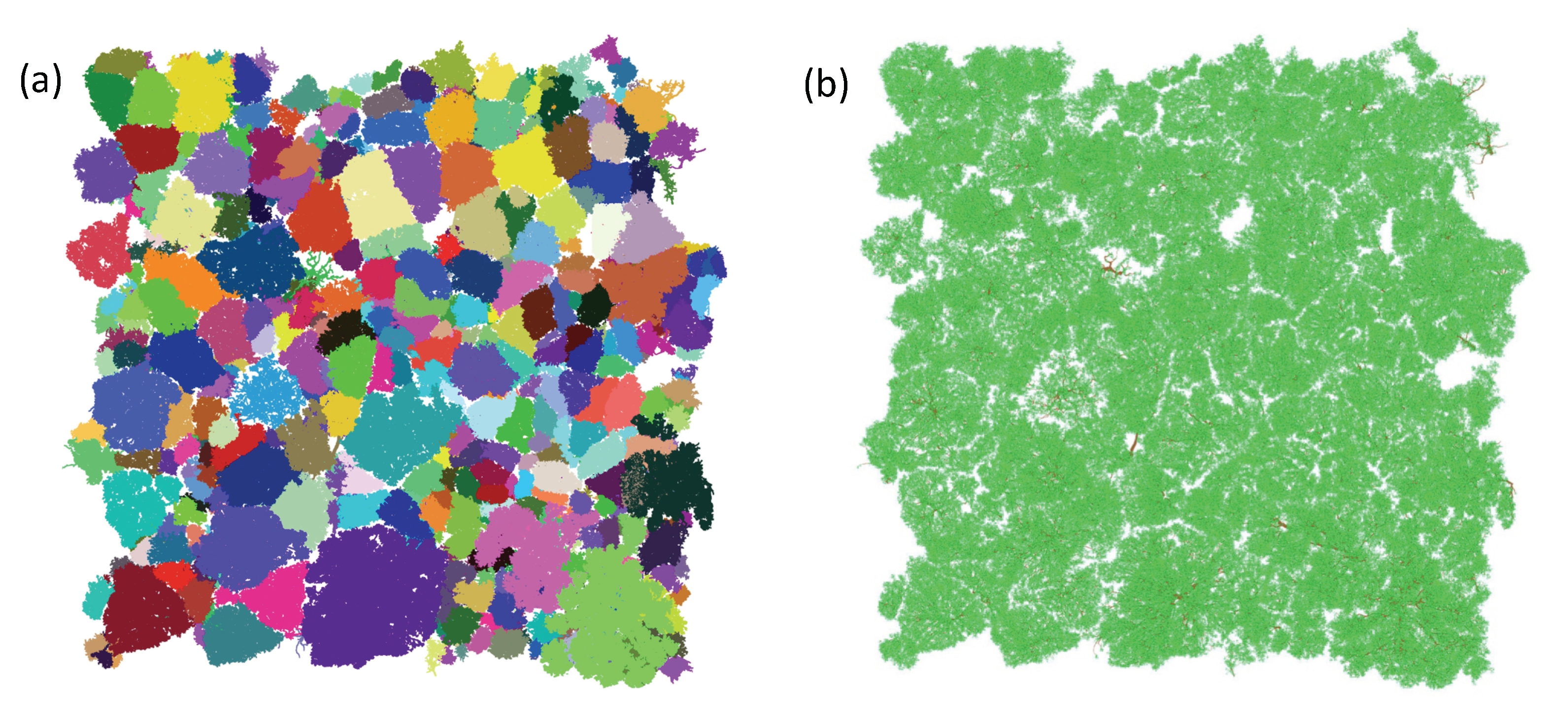
3.1. Forest Stand Reconstruction

We extracted 559 trees from the one hectare site in Wytham Woods. Figure 3 shows a side view of the segmented point cloud. The extracted trees from the TLS data were linked with the traditional census data collected in August 2016. A direct link was established for 483 trees. The 76 unlinked trees were generally small with an average height of 6.08 m and average DBH of 7.05 cm. For 35 of the unlinked trees, the species could be determined. These were generally multi-stem trees of which the species was known, but a direct match with a specific stem was not possible.

Gap fraction analysis of all 176 scan locations in leaf-on and leaf-off conditions determined that plot-level ePAI was 4.85 and eWAI was 1.89 [2]. Further analysis estimated that eLAI was 3.72 and the leaf area index was 3.8. Thirty trees within the stand were dead (based on the census data) and were not allocated any leaves. The 529 living tree QSMs had a total branch length of approximately 267.44 km. This ranged from 1.4 m to 11.9 km on a per-tree basis, with the average branching length per tree being 505.6 m. The relative branch length (i.e., the tree branch length divided by total plot branch length) was used to distribute the total leaf area of 38,000 m${}^2$ over the individual trees.

3D reconstructions of the branching architecture were performed for each tree individually. Figure 4b,c shows the optimised QSM for a Sycamore (Acer pseudoplatanus) tree. Figure 4d shows a fully leaf-on reconstructed Sycamore tree model. A rendering (using Blender, www.blender.org) of that tree was visualised in Figure A3, showing the leaf shape in detail. Colours are used to distinguish leaves (green) from branches (brown), not to reflect the tree’s radiometric properties. The full one hectare model is shown in Figure 5b (top view). It consists of 1.431 million individual leaves. Branching cylinders and leaves are stored in separate object files, allowing for easy leaf-off and leaf-on RT simulations.

3.2. Radiative Transfer Modelling

We simulated two different sensors using the librat RT model to demonstrate the use of the Wytham RT model: (a) an upward-looking in situ digital hemispherical photograph (DHP) and (b) a Sentinel-2 satellite image over the one hectare Wytham Woods model.

The DHP in Figure 6a was simulated using a version of the model which only includes the woody components (i.e., leaf-off winter scene) and the terrain. The camera model was based on a hemispherical image with a perfect cosine response. The spectral characteristics (i.e., spectral response function of the RGB channels) were modelled based on the Nikon D5100 using the dataset from Darrodi et al. [41]. The camera was placed in the scene at one metre above the terrain surface. We used a perfectly diffuse background illumination source where rays were tracked from the pixel array into the scene until they escaped. We sampled 300 rays per pixel in order to reduce the presence of noise. However, there is a direct trade-off between number of rays per pixel and the time required to simulate the whole image. The simulated image consisted of 811 × 811 pixels. Analysis of the DHPs was done similar to the methods described in Calders et al. [2]. eWAI was 1.58 for the simulated DHP (Figure 6a) and eWAI was 1.63 for the real DHP (Figure 6b) at approximately the same location. To account for small co-location errors between the simulated and real DHP, we also calculated a mean eWAI using 13 real DHPs that were located within an approximate 10 metres radius of the simulated image. The resulting real DHP mean eWAI of 1.56 with a standard deviation of 0.26 agrees well with the eWAI from the simulated image.

The images shown in Figure 7 show an aerial view of the central hectare of the full scene (i.e., leaf-on summer scene). Both RGB images are based on bands 2, 3 and 4 from the MSI instrument on Sentinel-2. A single illumination source was set that is equivalent to a 30${}^{\circ }$ solar zenith and 191${}^{\circ }$ solar azimuth angle. For Figure 7a the simulation was conducted at the native spatial resolution of those bands (10 m) using a camera placed at the same satellite orbit height (786 km). The equivalent distance, illumination and camera settings were used for Figure 7b whilst providing a spatial resolution equivalent to a 10 cm ground sampling distance. Both images were simulated using 30 rays per pixel.

3.3. Framework and Model Evaluation

Here we aim to present the 3D model and associated data, with a qualitative check of 3D model accuracy. Future work will provide a full quantitative validation via simulated data. Our approach is unique as it modelled all the individual trees from directly measured TLS data, rather than relying on a (limited) library of trees that are cloned and rotated. Burt et al. [25] reported a computing time of roughly one week for automated tree extraction of trees (DBH > 20 cm, 155 trees in total) in a one hectare tropical forest plot (24-core 2:40 GHz Intel Xeon E5-2620 v3 (15MB L3 cache) node with 72 Gb DDR4 RAM). Average tree structure model completion time in Calders et al. [15] was 102 s when using a Windows 7 64-bit operating system (3 .07 GHz, 24 GB memory). Åkerblom et al. [18] reported a computational time of 392 s (small oak) to 1099 s (large oak) for leaf generation with leaf area density distribution LADD 2 (quad-core IntelCore i7-6700K 4GHz, 32 Gb RAM). One of the limitations has been the ability of 3D RT models to be able to use these very detailed explicit 3D structural data. For the relatively few RT models around that can use explicit 3D data (e.g., librat, DART, raytran [3]) large scenes like this (comprising millions of unique objects) make simulations relatively slow, and the memory requirements are potentially very large. However, computational resources available to many researchers (i.e., large CPU clusters, multi-threading and massively parallel processing) have meant that virtual forest RT model approaches based on TLS data are now feasible.

While the reconstruction parameters are specific to the Wytham Woods case, the method is generic and easily adaptable and transferable to other ecosystems [25,42]. The modelling framework allows users to easily adjust parameters. This is especially important for the addition of leaves, where leaf shape and size, leaf area density distribution and leaf orientation distribution have a big influence on the simulated signal. Leaf-off TLS data allow for high quality QSMs, but these data are not available in many cases. Leaf-on data require leaf/wood separation [33] to extract the woody point cloud for QSM modelling. Leaf-on QSMs will generally have higher uncertainty towards the top of the trees due to occlusion in the data (e.g., see Figure 1 and [24,43]). Occlusion in the upper part of the canopy might not be a major issue for e.g., estimating above-ground biomass [15], but a good representation of the upper canopy is important for simulating airborne or spaceborne signals with radiative transfer models.

This modelling framework is transferable to other TLS instruments, assuming that the TLS data is of sufficient density and accuracy to represent the 3D structure of the canopy to the desired accuracy. This typically requires an instrument with a range of more than 100 m and beam divergence of a few cm at 100 m to resolve small branches [24]. A challenge is how to integrate 3D data available from a wider range of sources with different properties: lower cost, but lower range and precision TLS; UAV-mounted LiDAR; mobile LiDAR; photogrammetric point clouds via structure-from-motion. We suggest that proceeding from a “best-case” 3D RT scene model such as we present here may be a way to overcome this challenge. The virtual forest RT scene model can be used to simulate all of these data types. The resulting integration can then be developed and tested knowing the canopy properties a priori.

4. Conclusions

This paper describes the reconstruction of a virtual 3D radiative transfer model for a real forest based on terrestrial LiDAR data. Our method uses open-source algorithms and this general framework is highly transferable to data collected with other TLS instruments and different ecosystems. Furthermore, the 3D Wytham Woods model is of great value itself as it is, to our knowledge, the most explicitly modelled real forest to date. This highly detailed model is publicly available and can potentially advance algorithm development for upcoming spaceborne missions, as well as provide a realistic scene to test assumptions in current algorithms.

5. Data Availability

The Wytham 3D radiative transfer model is available from https://bitbucket.org/tree_research/wytham_woods_3d_model/.

References

1. Fang, H.; Wei, S.; Liang, S. Validation of MODIS and CYCLOPES LAI products using global field measurement data. Remote Sens. Environ. 2012, 119, 43–54. [Google Scholar] [CrossRef]
2. Calders, K.; Origo, N.; Disney, M.; Nightingale, J.; Woodgate, W.; Armston, J.; Lewis, P. Variability and bias in active and passive ground-based measurements of effective plant, wood and leaf area index. Agric. For. Meteorol. 2018, 252, 231–240. [Google Scholar] [CrossRef]
3. Widlowski, J.L.; Mio, C.; Disney, M.; Adams, J.; Andredakis, I.; Atzberger, C.; Brennan, J.; Busetto, L.; Chelle, M.; Ceccherini, G.; et al. The fourth phase of the radiative transfer model intercomparison (RAMI) exercise: Actual canopy scenarios and conformity testing. Remote Sens. Environ. 2015, 169, 418–437. [Google Scholar] [CrossRef] [Green Version]
4. Disney, M.; Lewis, P.; Gomez-Dans, J.; Roy, D.; Wooster, M.J.; Lajas, D. 3D radiative transfer modelling of fire impacts on a two-layer savanna system. Remote Sens. Environ. 2011, 115, 1866–1881. [Google Scholar] [CrossRef]
5. Calders, K.; Lewis, P.; Disney, M.; Verbesselt, J.; Herold, M. Investigating assumptions of crown archetypes for modelling LiDAR returns. Remote Sens. Environ. 2013, 134, 39–49. [Google Scholar] [CrossRef]
6. Schneider, F.D.; Leiterer, R.; Morsdorf, F.; Gastellu-Etchegorry, J.P.; Lauret, N.; Pfeifer, N.; Schaepman, M.E. Simulating imaging spectrometer data: 3D forest modeling based on LiDAR and in situ data. Remote Sens. Environ. 2014, 152, 235–250. [Google Scholar] [CrossRef]
7. Widlowski, J.L.; Côté, J.F.; Béland, M. Abstract tree crowns in 3D radiative transfer models: Impact on simulated open-canopy reflectances. Remote Sens. Environ. 2014, 142, 155–175. [Google Scholar] [CrossRef]
8. Lintermann, B.; Deussen, O. Interactive modelling of plants. IEEE Comput. Graph. 1999, 19, 2–11. [Google Scholar] [CrossRef]
9. Weber, J.; Penn, J. Creation and rendering of realistic trees. In Proceedings of the 22nd Annual Conference on Computer Graphics and Interactive Techniques, Los Angeles, CA, USA, 6–11 August 1995; pp. 119–128. [Google Scholar]
10. Armston, J.; Newnham, G.; Strahler, A.H.; Schaaf, C.; Danson, M.; Gaulton, R.; Zhang, Z.; Disney, M.; Sparrow, B.; Phinn, S.R.; et al. Intercomparison of Terrestrial Laser Scanning Instruments for Assessing Forested Ecosystems: A Brisbane Field Experiment. In Proceedings of the AGU Fall Meeting, San Fransico, CA, USA, 3–19 December 2013. [Google Scholar]
11. Woodgate, W.; Disney, M.; Armston, J.D.; Jones, S.D.; Suarez, L.; Hill, M.J.; Wilkes, P.; Soto-Berelov, M.; Haywood, A.; Mellor, A. An improved theoretical model of canopy gap probability for Leaf Area Index estimation in woody ecosystems. For. Ecol. Manag. 2015, 358, 303–320. [Google Scholar] [CrossRef]
12. Newnham, G.; Armston, J.; Calders, K.; Disney, M.; Lovell, J.; Schaaf, C.; Strahler, A.; Danson, F. Terrestrial Laser Scanning For Plot Scale Forest Measurement. Curr. For. Rep. 2015, 1, 239–251. [Google Scholar] [CrossRef]
13. Raumonen, P.; Kaasalainen, M.; Markku, A.; Kaasalainen, S.; Kaartinen, H.; Vastaranta, M.; Holopainen, M.; Disney, M.; Lewis, P. Fast automatic precision tree models from terrestrial laser scanner data. Remote Sens. 2013, 5, 491–520. [Google Scholar] [CrossRef]
14. Hackenberg, J.; Spiecker, H.; Calders, K.; Disney, M.; Raumonen, P. SimpleTree—An Efficient Open Source Tool to Build Tree Models from TLS Clouds. Forests 2015, 6, 4245–4294. [Google Scholar] [CrossRef]
15. Calders, K.; Newnham, G.; Burt, A.; Murphy, S.; Raumonen, P.; Herold, M.; Culvenor, D.; Avitabile, V.; Disney, M.; Armston, J.; et al. Nondestructive estimates of above-ground biomass using terrestrial laser scanning. Methods Ecol. Evol. 2015, 6, 198–208. [Google Scholar] [CrossRef]
16. Côté, J.F.; Widlowski, J.L.; Fournier, R.A.; Verstraete, M.M. The structural and radiative consistency of three-dimensional tree reconstructions from terrestrial lidar. Remote Sens. Environ. 2009, 113, 1067–1081. [Google Scholar] [CrossRef] [Green Version]
17. Côté, J.F.; Fournier, R.A.; Egli, R. An architectural model of trees to estimate forest structural attributes using terrestrial LiDAR. Environ. Modell. Softw. 2011, 26, 761–777. [Google Scholar] [CrossRef]
18. Åkerblom, M.; Raumonen, P.; Casella, E.; Disney, M.; Danson, F.; Gaulton, R.; Schofield, L.A.; Kaasalainen, M. Non-Intersecting leaf insertion algorithm for tree structure models. Interface Focus 2018, 8, 20170045. [Google Scholar] [CrossRef] [PubMed]
19. Côté, J.F.; Fournier, R.A.; Frazer, G.W.; Niemann, K.O. A fine-scale architectural model of trees to enhance LiDAR-derived measurements of forest canopy structure. Agric. For. Meteorol. 2012, 166–167, 72–85. [Google Scholar] [CrossRef]
20. Butt, N.; Campbell, G.; Malhi, Y.; Morecroft, M.; Fenn, K.; Thomas, M. Initial Results from Establishment of a Long-Term Broadleaf Monitoring Plot at Wytham Woods; University of Oxford: Oxford, UK, 2009. [Google Scholar]
21. Lovell, J.L.; Jupp, D.L.B.; Culvenor, D.S.; Coops, N.C. Using airborne and ground-based ranging lidar to measure canopy structure in Australian forests. Can. J. Remote Sens. 2003, 29, 607–622. [Google Scholar] [CrossRef]
22. Calders, K.; Armston, J.; Newnham, G.; Herold, M.; Goodwin, N. Implications of sensor configuration and topography on vertical plant profiles derived from terrestrial LiDAR. Agric. For. Meteorol. 2014, 194, 104–117. [Google Scholar] [CrossRef]
23. Calders, K.; Burt, A.; Origo, N.; Disney, M.; Nightingale, J.; Raumonen, P.; Lewis, P. Large-area virtual forests from terrestrial laser scanning data. In Proceedings of the IEEE International Geoscience and Remote Sensing Symposium (IGARSS), Beijing, China, 10–15 July 2016; pp. 1765–1767. [Google Scholar]
24. Wilkes, P.; Lau, A.; Disney, M.; Calders, K.; Burt, A.; de Tanago, J.G.; Bartholomeus, H.; Brede, B.; Herold, M. Data acquisition considerations for Terrestrial Laser Scanning of forest plots. Remote Sens. Environ. 2017, 196, 140–153. [Google Scholar] [CrossRef]
25. Burt, A.; Disney, M.; Calders, K. Extracting individual trees from lidar point clouds using treeseg. Methods Ecol. Evol. 2018. in review. [Google Scholar]
26. Burt, A. New 3D Measurements of Forest Structure. Ph.D. Thesis, University College London, London, UK, 2017. [Google Scholar]
27. Rusu, R.B.; Cousins, S. 3D is here: Point Cloud Library (PCL). In Proceedings of the IEEE International Conference on Robotics and Automation (ICRA), Shanghai, China, 9–13 May 2011. [Google Scholar]
28. Calders, K.; Disney, M.I.; Armston, J.; Burt, A.; Brede, B.; Origo, N.; Muir, J.; Nightingale, J. Evaluation of the Range Accuracy and the Radiometric Calibration of Multiple Terrestrial Laser Scanning Instruments for Data Interoperability. IEEE Trans. Geosci. Remote Sens. 2017, 55, 2716–2724. [Google Scholar] [CrossRef] [Green Version]
29. Juchheim, J.; Annighöfer, P.; Ammer, C.; Calders, K.; Raumonen, P.; Seidel, D. How management intensity and neighborhood composition affect the structure of beech (Fagus sylvatica L.) trees. Trees 2017, 31, 1723–1735. [Google Scholar] [CrossRef]
30. Åkerblom, M.; Raumonen, P.; Kaasalainen, M.; Casella, E. Analysis of Geometric Primitives in Quantitative Structure Models of Tree Stems. Remote Sens. 2015, 7, 4581–4603. [Google Scholar] [Green Version]
31. Calders, K.; Newnham, G.; Herold, M.; Murphy, S.; Culvenor, D.; Raumonen, P.; Burt, A.; Armston, J.; Avitabile, V.; Disney, M. Estimating above ground biomass from terrestrial laser scanning in Australian Eucalypt Open Forest. In Proceedings of the 2013 SilviLaser, Beijing, China, 9–11 October 2013; pp. 90–97. [Google Scholar]
32. Calders, K.; Burt, A.; Newnham, G.; Disney, M.; Murphy, S.; Raumonen, P.; Herold, M.; Culvenor, D.; Armston, J.; Avitabile, V.; et al. Reducing uncertainties in above-ground biomass estimates using terrestrial laser scanning. In Proceedings of the 2015 SilviLaser, La Grande Motte, France, 28–30 September 2015; pp. 197–199. [Google Scholar]
33. Disney, M.; Boni Vicari, M.; Burt, A.; Calders, K.; Lewis, S.L.; Raumonen, P.; Wilkes, P. Weighing trees with lasers: advances, challenges and opportunities. Interface Focus 2018, 8, 20170048. [Google Scholar] [CrossRef] [PubMed] [Green Version]
34. Jupp, D.L.B.; Culvenor, D.S.; Lovell, J.L.; Newnham, G.J.; Strahler, A.H.; Woodcock, C.E. Estimating forest LAI profiles and structural parameters using a ground-based laser called Echidna®. Tree Physiol. 2009, 29, 171–181. [Google Scholar] [CrossRef] [PubMed]
35. Calders, K.; Schenkels, T.; Bartholomeus, H.; Armston, J.; Verbesselt, J.; Herold, M. Monitoring spring phenology with high temporal resolution terrestrial LiDAR measurements. Agric. For. Meteorol. 2015, 203, 158–168. [Google Scholar] [CrossRef]
36. Ryu, Y.; Nilson, T.; Kobayashi, H.; Sonnentag, O.; Law, B.E.; Baldocchi, D.D. On the correct estimation of effective leaf area index: Does it reveal information on clumping effects? Agric. For. Meteorol. 2010, 150, 463–472. [Google Scholar] [CrossRef]
37. Lewis, P. Three-dimensional plant modelling for remote sensing simulation studies using the Botanical Plant Modelling System. Agron. Agric. Environ. 1999, 19, 185–210. [Google Scholar] [CrossRef]
38. Pinty, B.; Widlowski, J.L.; Taberner, M.; Gobron, N.; Verstraete, M.M.; Disney, M.; Gascon, F.; Gastellu, J.P.; Jiang, L.; Kuusk, A.; et al. Radiation Transfer Model Intercomparison (RAMI) exercise: Results from the second phase. J. Geophys. Res. 2004, 109, D06210. [Google Scholar] [CrossRef]
39. Widlowski, J.L.; Taberner, M.; Pinty, B.; Bruniquel-Pinel, D.; Disney, M.; Fernandes, R.; Gastellu-Etchegorry, J.P.; Gobron, N.; Kuusk, A.; Lavergne, T.; et al. Third Radiation transfer Model Intercomparison (RAMI) exercise: Documenting progress in canopy reflectance models. J. Geophys. Res. 2007, 112, D09111. [Google Scholar] [CrossRef]
40. Disney, M.I.; Kalogirou, V.; Lewis, P.; Prieto-Blanco, A.; Hancock, S.; Pfeifer, M. Simulating the impact of discrete-return lidar system and survey characteristics over young conifer and broadleaf forests. Remote Sens. Environ. 2010, 114, 1546–1560. [Google Scholar] [CrossRef]
41. Darrodi, M.M.; Finlayson, G.; Goodman, T.; Mackiewicz, M. Reference data set for camera spectral sensitivity estimation. J. Opt. Soc. Am. A 2015, 32, 381–391. [Google Scholar] [CrossRef] [PubMed]
42. Gonzalez de Tanago, J.; Lau, A.; Bartholomeus, H.; Herold, M.; Avitabile, V.; Raumonen, P.; Martius, C.; Goodman, R.C.; Disney, M.; Manuri, S.; et al. Estimation of above-ground biomass of large tropical trees with terrestrial LiDAR. Methods Ecol. Evol. 2018, 9, 223–234. [Google Scholar] [CrossRef]
43. Kükenbrink, D.; Schneider, F.D.; Leiterer, R.; Schaepman, M.E.; Morsdorf, F. Quantification of hidden canopy volume of airborne laser scanning data using a voxel traversal algorithm. Remote Sens. Environ. 2017, 194, 424–436. [Google Scholar] [CrossRef]
Figure 1. Terrestrial laser scanning (TLS) data acquisition in Wytham Woods (a) TLS cross-section of 200 m transect in leaf-on conditions; (b) TLS cross-section of 200 m transect in leaf-off conditions.
Remotesensing 10 00933 g001
Figure 2. Leaf shape.
Remotesensing 10 00933 g002
Figure 3. Segmented one hectare point cloud of Wytham Woods: 559 individual trees were extracted.
Remotesensing 10 00933 g003
Figure 4. Reconstruction of a Sycamore (Acer pseudoplatanus) tree. (a) TLS leaf-off point cloud coloured by height (note that this multi-stem tree splits below 1.3 m and is therefore considered to be two trees in the analysis); (b) TLS leaf-off point cloud overlaid with QSM; (c) QSM; (d) Fully reconstructed tree: QSM + added leaves.
Remotesensing 10 00933 g004
Figure 5. Full one hectare model of Wytham Woods. (a) Top view of segmented TLS point cloud (b) Top view of radiative transfer input model: QSMs for branching architecture + leaves.
Remotesensing 10 00933 g005
Figure 6. Simulated and real upward-looking in situ digital hemispherical photograph (DHP) in Wytham Woods at approximately the same location. (a) Simulated in-situ DHP using the Wytham Woods leaf-off scene model (b) Real in-situ DHP (see Calders et al. [2] for details of image acquisition).
Remotesensing 10 00933 g006
Figure 7. Simulated Sentinel-2 satellite image over the one hectare Wytham Woods model. (a) 10 m spatial resolution image (100 pixels); (b) 10 cm ground sampling distance (1 megapixel).
Remotesensing 10 00933 g007