Multiscale and Multi-Granularity Process Analytics: A Review

Abstract

As Industry 4.0 makes its course into the Chemical Processing Industry (CPI), new challenges emerge that require an adaptation of the Process Analytics toolkit. In particular, two recurring classes of problems arise, motivated by the growing complexity of systems on one hand, and increasing data throughput (i.e., the product of two well-known “V’s” from Big Data: Volume × Velocity) on the other. More specifically, as enabling IT technologies (IoT, smart sensors, etc.) enlarge the focus of analysis from the unit level to the entire plant or even to the supply chain level, the existence of relevant dynamics at multiple scales becomes a common pattern; therefore, multiscale methods are called for and must be applied in order to avoid biased analysis towards a certain scale, compromising the benefits from the balanced exploitation of the information content at all scales. Also, these same enabling technologies currently collect large volumes of data at high-sampling rates, creating a flood of digital information that needs to be properly handled; optimal data aggregation provides an efficient solution to this challenge, leading to the emergence of multi-granularity frameworks. In this article, an overview is presented on multiscale and multi-granularity methods that are likely to play an important role in the future of Process Analytics with respect to several common activities, such as data integration/fusion, de-noising, process monitoring and predictive modelling, among others.

1. Introduction

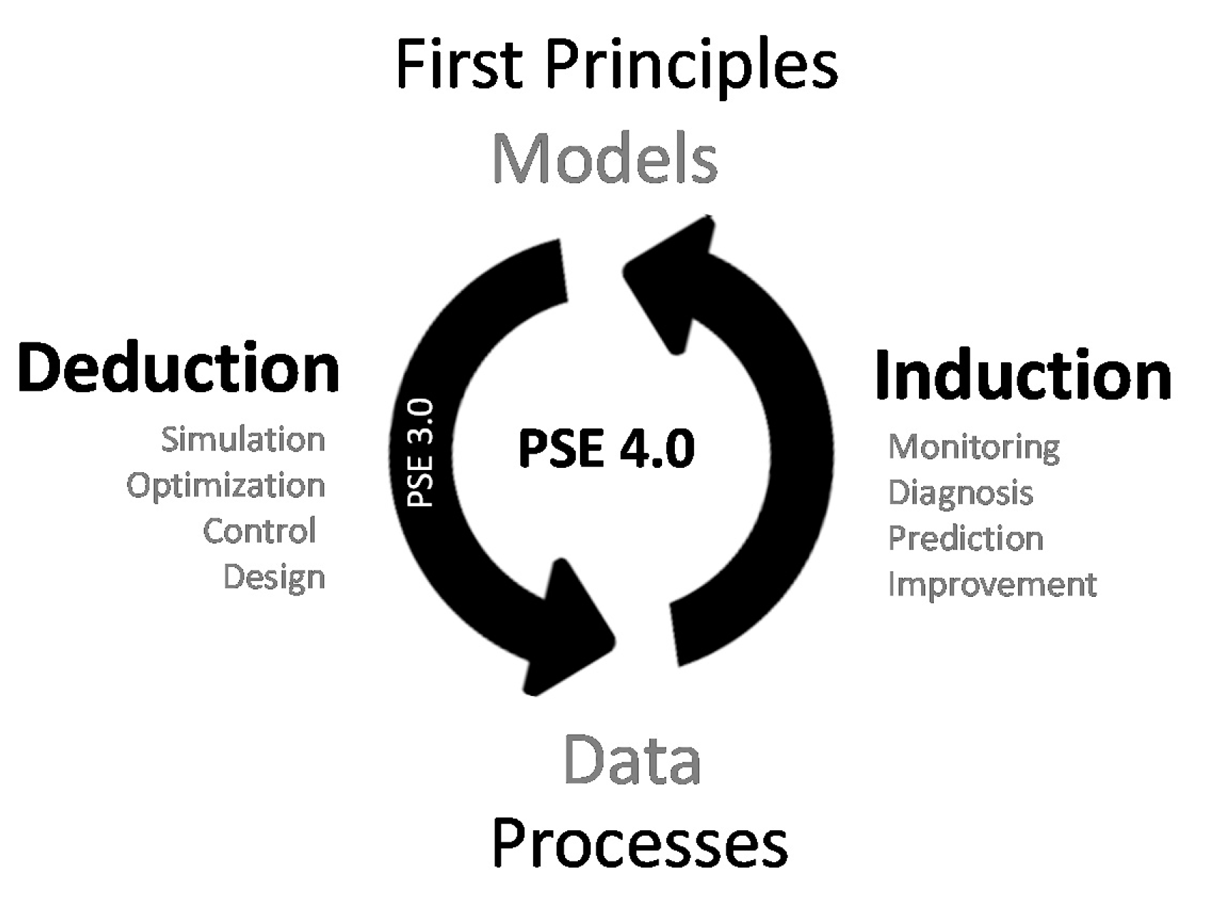
Process Systems Engineering (PSE) emerged during the 3rd industrial revolution and allowed Chemical Engineers to take advantage of computational power to put into action their knowledge about process phenomena through first principle model-based deductive approaches. With the dawn of the fourth industrial revolution, computers are again pillars of a new technological shift that consists of extracting knowledge from abundant process data, rather than acting as repositories of existing knowledge carefully programmed by Engineers. Therefore, the classical deductive PSE perspective can now be properly complemented with data-centric inductive methods, enlarging its scope and setting the ground for the challenges modern industry is currently facing. This new deductive-inductive integrated perspective can be properly coined as PSE 4.0 (Figure 1). Much like optimization, numerical analysis, computing, and mathematics provided the conceptual framework for Chemical Engineers to establish PSE 3.0, data science, machine learning, high performance computing (HPC), and high-dimensional statistics are currently structuring the inductive branch of PSE 4.0.

Data-driven and evidence-based analysis is growing in importance as a critical task in the context of process operations in the Chemical Processing Industry (CPI) [1,2,3,4]. Among the several categories of challenges PSE is facing nowadays [3], two stand out: handling systems complexity and the ability to cope with increasing data throughput. More than ever before, data is being collected from different points of the supply chain, each one of them having the potential for leaving a fingerprint on final product quality. These sub-processes span several time scales: from second/minutes at the equipment level, to hours/days and the units level, days/months at the plant level, and even months/years at the supply chain level. Different phenomena taking place at these scales brings up potentially relevant aspects for improving product quality and therefore should be analyzed and properly exploited. However, for that to happen, the available single-scale tools that are focused in a single “most representative” scale, must be replaced by multiscale methods that are able to provide a balanced and commensurate importance to all time scales, without biasing the analysis towards one of them. This is the main goal of multiscale approaches, whose opportunity and relevance gains a new dimension nowadays.

On the other hand, once companies begin exploiting the plethora of data sources available and the volume of information collected from all of them, they quickly realize that traditional data analysis methods are ineffective and do not scale well with data increasing volume. In this setting, a common quick fix that has been adopted so far is to throw overboard some data under the assumption that processes are oversampled and nothing meaningful would be lost by discarding a part of it. Sub-sample and multirate schemes fall in this category [5,6,7,8,9,10,11,12,13,14,15,16]. However, an alternative approach is gaining importance: data aggregation. Instead of simply discarding data, these methods aggregate them according to a rational or optimality criterion in a certain pre-defined sense. In this situation, partial information from all observations is retained and at the same time the amount of data analyzed is greatly reduced. These methods are called multiresolution or multi-granularity, and are newcomers to the Process Analytical toolkit.

In this article, an overview is provided on the current state-of-the-art methodologies for handling the complex multiscale dynamic nature of industrial processes and for performing multi-granularity analysis. The focus is on data-centric inductive methods and therefore the model-based deductive approaches will not be covered (some examples of model-based multiscale approaches can be found in [17,18,19,20,21]). With the exception of a review paper dedicated to multiscale monitoring methods from 2004 [22], no work was hitherto published, reviewing and discussing multiscale and multiresolution data-driven methods. The present article fills a gap in the technical literature and at the same time brings out methods whose importance is likely to grow as Industry 4.0 generates more data and with higher complexity.

In the next section, multiscale approaches are revised according to their application scope. Then, we move to the presentation of the more recent multi-granularity methods, where both the analysis of multiresolution data and the creation of multiresolution data structures are covered and discussed. The article ends with a brief overview of the topics presented and perspective thoughts for their role in the future of Process Analytics.

2. Multiscale Methods

Modern industrial processes are highly integrated and intensified, with different phenomena going on at different locations and interacting in complex ways. These phenomena span different scales of time and their signatures are left imprinted in data collected through the plethora of process instrumentation currently available: sensors, Process Analytical Technology (PAT) devices, chromatograms, thermal/hyperspectral images, particle size distributions, etc. Single-scale techniques are focused on the analysis of phenomena at one scale, usually the one regarding the sampling rate. Therefore, they are limited in the amount of information they can extract from process data exhibiting multiscale phenomena. In more technical terms, the concept of “scale” is associated with a subdivision of the frequency spectrum in bands. Higher (or coarser) scales are related to lower frequency bands and lower (or finer) scales, to high-frequency bands. A possible definition of “scale” is the following: a series of non-overlapping (or partially overlapping) frequency bands that, when combined, cover the entire frequency spectrum for the system under analysis; each frequency band represents a given scale and is usually indexed by an integer number: the usual convention is that lower numbers correspond to finer scales and larger numbers to coarser scales. In this context, there is a relationship between the scale index, a characteristic range of frequencies and the relevant time/length periods.

In multiscale data analysis, several mathematical, computational and statistical methods are adopted to efficiently describe the occurrence of events in distinct locations and with different localizations in the time-frequency plane [23,24] (location regards “where” a given event happens in time or in the frequency axis, whereas localization refers to the degree of “dispersion” in these domains). A fundamental component of the multiscale framework is the ability to zoom in into the different scales of interest. Examples of enabling methodologies for this critical activity include wavelet theory, and, more recently, the Empirical Mode Decomposition (EMD) and Hilbert-Huang transform (HHT) and [25,26,27]. These later methods provide alternative ways to perform the multiscale decomposition to the more pervasive wavelet transform. EMD adaptively establishes the decomposition functions (called intrinsic mode functions) directly from data, instead of using a fix wavelet function across the entire analysis; therefore, this algorithm is claimed to be a better choice for handling data collected from non-stationary processes. HHT is an evolution of EMD, where an additional processing step is applied to the intrinsic mode functions (Hilbert spectral analysis) in order to obtain instantaneous frequency information. Among these decomposition frameworks, the wavelet transform largely dominated the publication landscape over the years, and therefore will be referred here more extensively. A brief overview of wavelet theory is provided in the next subsection. The interested reader can easily find plenty of sources for more information on this topic, such as introductory texts [28,29,30,31,32], more thorough treatments [33,34], mathematically-oriented manuscripts [35,36,37], material reporting a wide variety of applications [38,39,40,41,42,43], and more technically advanced treatments [44], as well as a variety of review articles [45,46].

2.1. Fundamentals of Wavelet Theory

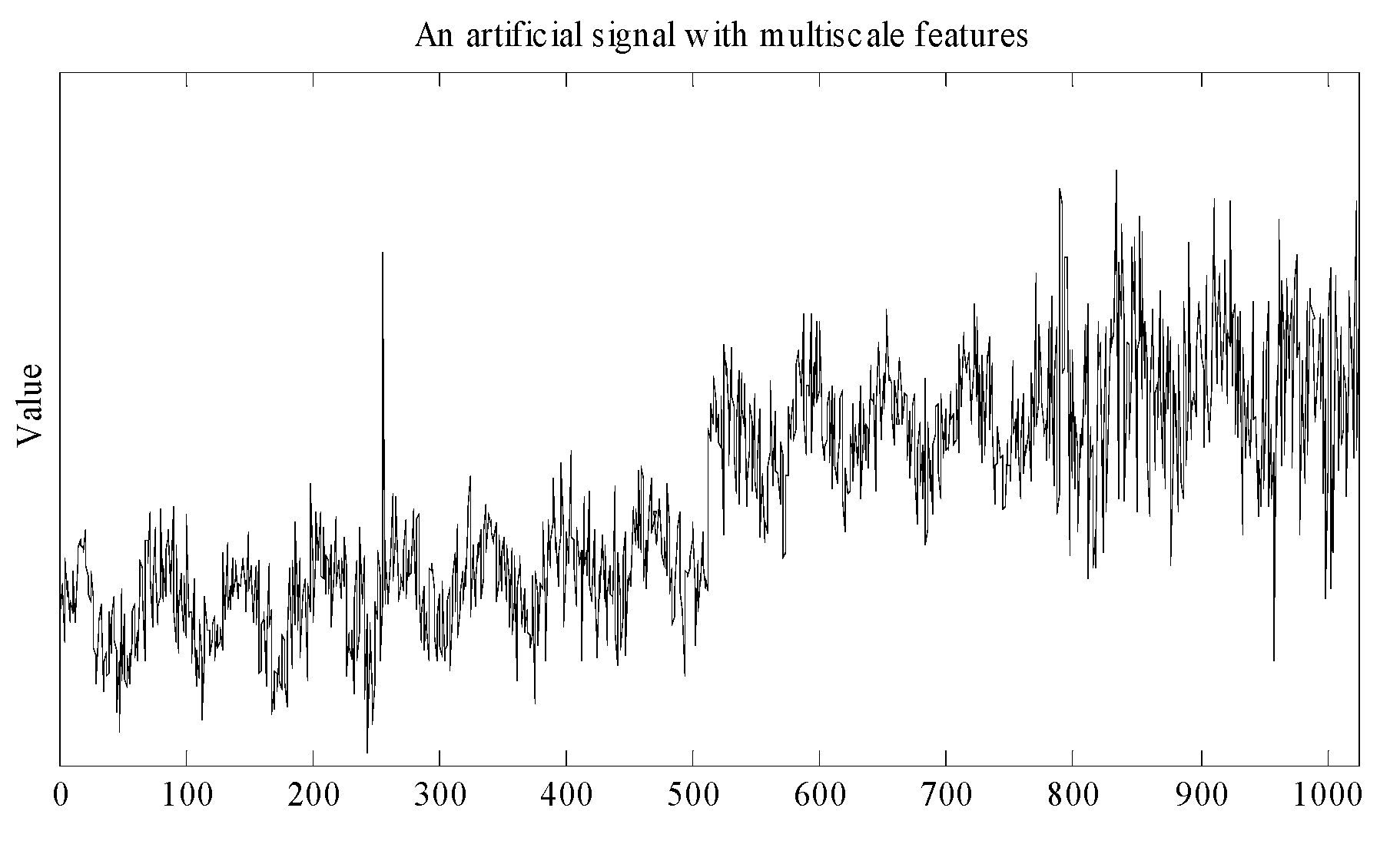
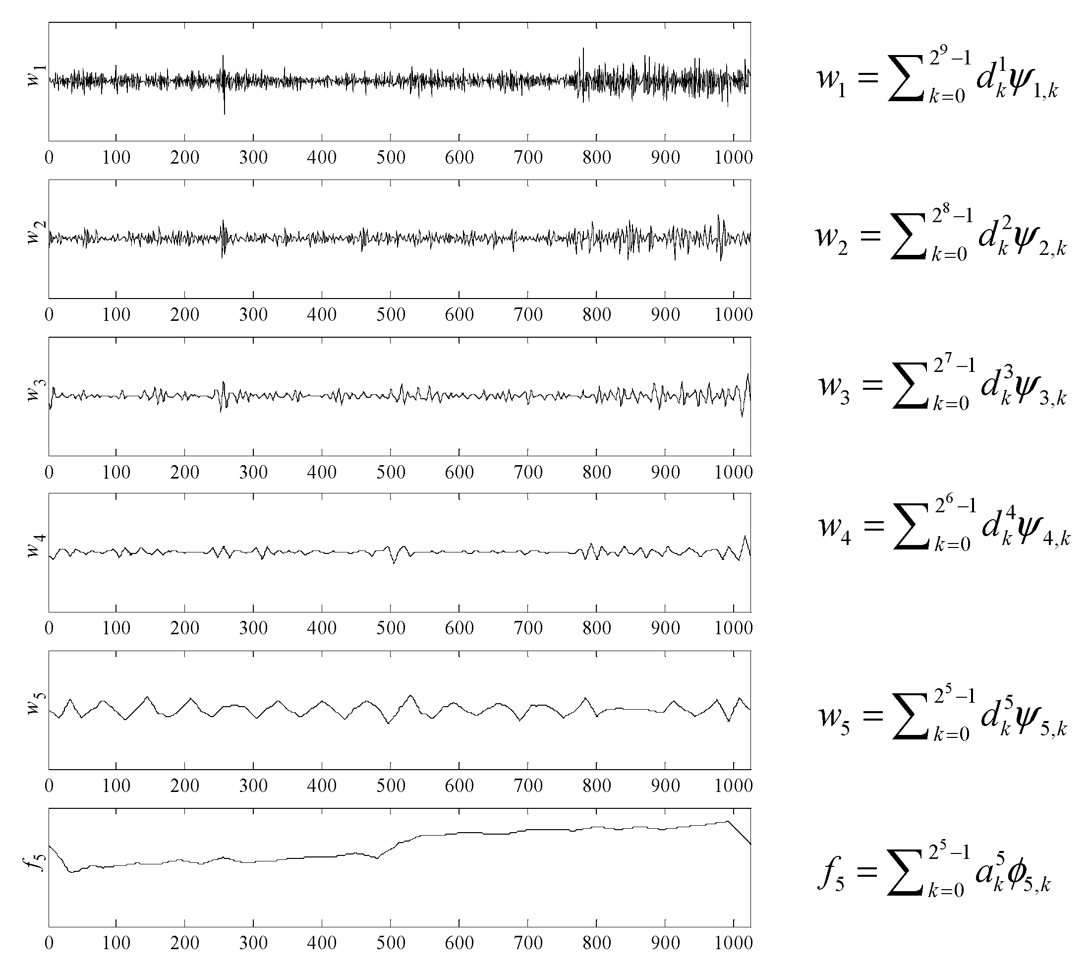
Data acquired from industry often present complex patterns with features appearing at different locations and with different localizations either in time and frequency [23]. The signal presented in Figure 2 was constructed to illustrate this point: it is composed by superimposing several deterministic and stochastic features, each one of which with its own characteristic time/frequency pattern. The signal deterministic features consist of a ramp that begins right from the start, a step perturbation at sample 513, a permanent oscillatory component, and a spike at observation number 256. The stochastic feature consists of additive Gaussian white noise, whose variance increases after sample number 768. Clearly these events have different time/frequency locations and localizations. For instance, the spike is completely localized in time, but fully delocalized in the frequency domain; on the other hand, the sinusoidal component is highly concentrated is a narrow region of the frequency domain but its time representation spreads over the whole time axis. White noise contains contributions from all frequencies and its energy is uniformly distributed in the time/frequency plane. The linear trend is essentially a low frequency perturbation, and its energy is almost entirely concentrated in the lower frequency bands. All of these patterns appear simultaneously in the signal, and may leave their fingerprint on the final product quality. Therefore, they should be given equal opportunities in the course of analysis and their effects should be assessed without compromising one kind of feature over the others. This can only be done, however, by adopting suitable mathematical frameworks for efficiently describing data with multiscale characteristics. Wavelet theory provides one such framework, and will be briefly reviewed in this section.

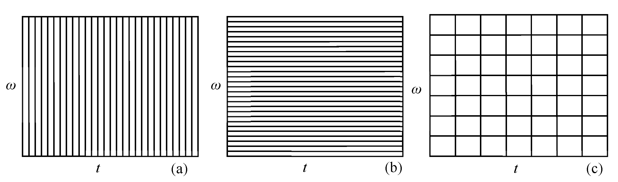
Transforms, like the Fourier or Wavelet transforms, provide alternative ways for representing raw data. The alternative representations consist of expansions of basis functions multiplied by coefficients. The expansion coefficients constitute the transform, and, if the methodology is properly chosen, only a few of them are necessary to capture the main features in data. For instance, Fourier transform is the adequate mathematical framework for describing periodic phenomena or smooth signals, since the nature of its basis functions allows for compact representations of such trends. In other words, only a few Fourier transform coefficients are required to provide a good basis expansion representation of the original periodic signals. The same applies, in other contexts, to other classical single-scale linear transforms [23,33,35], such as the one based on the discrete Dirac-δ function or the windowed Fourier transform. However, none of these single-scale linear transforms are able to cope effectively with the diversity of features present in signals such as the one illustrated in Figure 2. A proper analysis of this signal, using any of these techniques, would require a large number of coefficients to capture all stochastic and deterministic features, indicating that they are not adequate mathematical frameworks for handling signals with multiscale features such as this one: they do not enable a compact translation of key features in the transform domain. This happens because the form of the time/frequency windows [33,41], associated with their basis functions (Figure 3), does not change across the time/frequency plane in such a way as would be required to effectively cover the localized high energy zones of the several features present in the signal.

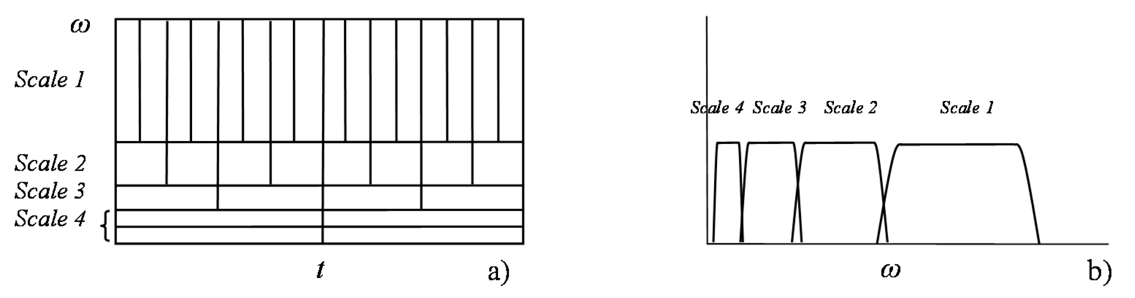
In order to cope with multiscale features, a more flexible tiling of the time/frequency space is necessary. This coverage is provided by the wavelet transform, where wavelets are adopted as basis functions (Figure 4) and the associated expansion coefficients form the wavelet transform. In practice, it is often the case that signals are composed of short duration events at high frequency and low frequency events with longer durations. This is exactly the kind of tilling wavelet basis functions are able to provide, since their relative frequency bandwidth is a constant. In other words, the ratio between a measure of the size of the frequency band and the mean frequency, $\Delta \omega /\omega$, is constant for each wavelet function, which is known as the constant-Q property [46].

Wavelets are particular types of functions whose location and localization characteristics in time/frequency are ruled by two parameters: both the localization in this plane and location in the frequency domain are determined by the scale parameter, s; the location in the time domain is controlled by the time translation parameter, b. Each wavelet, ${\psi }_{s,b}\left(t\right)$, can be obtained from the so-called “mother wavelet”, $\psi \left(t\right)$, through a scaling operation (that “stretches” or “compresses” the original function, establishing its form), and a translation operation (that controls its positioning in the time axis):

$${\psi }_{s,b}\left(t\right)=\frac{1}{\sqrt{\left|s\right|}}\psi \left(\frac{t-b}{s}\right)$$

(1)

The shape of the mother wavelet is such that it has an equal area above and below the time axis, which means that, besides having a compact localization in this axis, they oscillate around it (hence its name “wavelets”, i.e., small waves). In the Continuous Wavelet Transform (CWT), scale and translation parameters can vary continuously, leading to a redundant transform (a 1D signal is being mapped onto a 2D function). Therefore, in order to construct a basis set, the continuous wavelet transform is appropriately sampled so that the set of wavelet functions parameterized by the new discrete indices (scale index, j, and translation or shift index, k) cover the time-frequency plane in a non-redundant way. This sampling consists of applying a dyadic grid in which b is sampled more frequently for lower values of s, while s grows exponentially with the power of 2:

$${\psi }_{j,k}(t)={\psi }_{s,b}{(t)}_{|\begin{array}{c}s=2^j\\ b=k·2^j\end{array}}=\frac{1}{2^{j/2}}\psi \left(\frac{t-k·2^j}{2^j}\right)=\frac{1}{2^{j/2}}\psi \left(\frac{t}{2^j}-k\right)$$

(2)

The set of wavelet functions in (2) forms a basis for the space of all square integrable functions, $L^2\left(ℝ\right)$ [47]. However, in data analysis, users have to deal with discretized data (data tables, images, spectra, etc.), which have finite dimensionality. Still, it is possible to compute the wavelet transform for these entities through the scheme known as Multiresolution Decomposition Analysis, developed by Stephane Mallat [33,48].

Multiresolution Decomposition Analysis is theoretically framed in the mathematical concept of Multiresolution Approximation, through which a signal available at the finest resolution, $f_0$, can be represented by its approximation at a coarser resolution ($f_j$), plus all details that are lost when moving from $f_0$ to $f_j$, and that are relative to the scales in between ${\left\{w_i\right\}}_{i=1:j}$. These coarser approximations and details at different scales correspond to projections into approximation, $V_j$, and detail spaces, ${\left\{W_i\right\}}_{i=1:j}$, as follows:

$$f_0=f_j+{\displaystyle \sum _{i=1}^j{w}_i}\iff f_0={\mathrm{Pr}}_{V_j}{f}_0+{\displaystyle \sum _{i=j}^1{\mathrm{Pr}}_{W_i}{f}_0}$$

(3)

It can be shown that an orthonormal basis for the details space $W_j$ is given by the set of wavelet functions, ${\left\{{\psi }_{j,k}\right\}}_{k\in \mathbb{Z}}$. These basis sets (for different scales) are mutually orthogonal, as they span orthogonal subspaces of $L^2\left(ℝ\right)$. Therefore, the projections, $f_j$ and ${\left\{w_i\right\}}_{i=1,\dots ,j}$ in (3), can adequately be written in terms of the linear combination of basis functions (4) multiplied by the expansion coefficients, calculated as inner products of the signal and basis functions (5).

$$f_0={\displaystyle \sum _k{a}_k^j{\varphi }_{j,k}}+{\displaystyle \sum _{i=1}^j{\displaystyle \sum _k{d}_k^i{\psi }_{i,k}}}$$

(4)

where

$$a_k^j=\langle f_j,{\varphi }_{j,k}\rangle ,d_k^i=\langle f_j,{\psi }_{i,k}\rangle$$

(5)

These coefficients are usually referred to as the (discrete) wavelet transform or wavelet coefficients:

• Approximation coefficients:$a_k^j(k\in \mathbb{Z})$;
• Details coefficients:$d_k^i(i=1,\dots ,j;k\in \mathbb{Z})$.

Mallat (1989) proposed a very efficient recursive scheme for the computation of wavelet coefficients, Equations (6) and (7), as well as for signal reconstruction, Equation (8), that essentially consists of implementing a pyramidal algorithm, based upon convolution with quadrature mirror filters, a well-known technique in the engineering discrete signal processing community:

• Signal analysis or decomposition

  $$a_k^{j+1}={\displaystyle \sum _n{h}_{n-2k}·a_n^j}$$

  (6)

  $$d_k^{j+1}={\displaystyle \sum _n{g}_{n-2k}·a_n^j}$$

  (7)
• Signal synthesis or reconstruction

  $$a_k^j={\displaystyle \sum _n{h}_{k-2n}·a_n^{j+1}}+{\displaystyle \sum _n{g}_{k-2n}·d_n^{j+1}}$$

  (8)

  where ${\left\{h_i\right\}}_{i\in \mathbb{Z}}$ and ${\left\{g_i\right\}}_{i\in \mathbb{Z}}$ are the low-pass and high-pass filter coefficients, respectively, whose values are closely related [31,33,34,44].

As an illustration, let us decompose the signal presented in Figure 2 that contains $2^{10}$ points at scale $j=0$, into a coarser, lower resolution, high granularity version at scale $j=5$ with $2^5$ approximation coefficients appearing in the expansion ($f_5={\displaystyle {\sum }_{k=0}^{2^5-1}{a}_k^5{\varphi }_{5,k}}$), plus all the detail signals from scale $j=1$ (with $2^9$ detail coefficients, $w_1={\displaystyle {\sum }_{k=0}^{2^9-1}{d}_k^1{\psi }_{1,k}}$) until scale $j=5$ (with $2^5$ detail coefficients, $w_5={\displaystyle {\sum }_{k=0}^{2^5-1}{d}_k^1{\psi }_{5,k}}$). The total number of wavelet coefficients is equal to the cardinality of the original signal. Thus, no information was “created” or “disregarded”, but simply transformed ($2^{10}=2^5+2^5+2^6+\cdots +2^9$). The projections onto the approximation and detail spaces are presented in Figure 5, where it is possible to observe that the deterministic and stochastic features appear quite clearly separated, according to their time/frequency location and localization: coarser deterministic features (ramp and step perturbation) appear in the coarser version of the signal (containing the lower frequency contributions), the sinusoid is captured in the detail at scale $j=5$, noise features appearing quite clearly at high frequency bands (details for $j=1,2$) where the increase of variance is noticeable, as well as the spike at observation 256 (another high frequency perturbation). This illustrates the ability of wavelet transforms to separate deterministic and stochastic contributions present in a signal, according to their time/frequency locations.

This flexibility offered by the wavelet representation is exploited in multiscale data analysis methods. The following properties of the wavelet transform are particularly relevant and justify their widespread adoption as the mathematical language for data-driven multiscale methods:

• Energy compaction property. The shifting/dilation properties of wavelet basis functions make them flexible enough to efficiently describe localized features with distinct patterns in the time-frequency plane. Therefore, wavelet transforms are able to extract the deterministic features in a few wavelet coefficients, which is an interesting characteristic for feature extraction [44,45,46,47,48,49], compression [50,51,52,53,54,55], and denoising applications [56,57,58,59,60].
• Decorrelation property. By application of the wavelet transform, stochastic autocorrelated processes spread their power spectra across the different scales of wavelet coefficients (frequency bands) and the sequences of wavelet coefficients at each scale become approximately decorrelated. In other words, the autocorrelation matrices of the original data are approximately diagonalized by the wavelet transform [19,36,61]. This enables the development of advanced multiscale process monitoring methods [62,63,64] and predictive modelling approaches [65,66,67,68,69,70].
• Computational efficiency. The computations involved are simple and fast (computation complexity of $O\left(N\right)$), and therefore can be easily implemented in any computational platform or hardware, for both offline and online applications.

These properties are explored differently in the variety of application scenarios of multiscale methods. In the next subsections, a brief overview is provided of multiscale frameworks designed for addressing relevant problems in practice.

2.2. Multiscale Methods for Process Monitoring

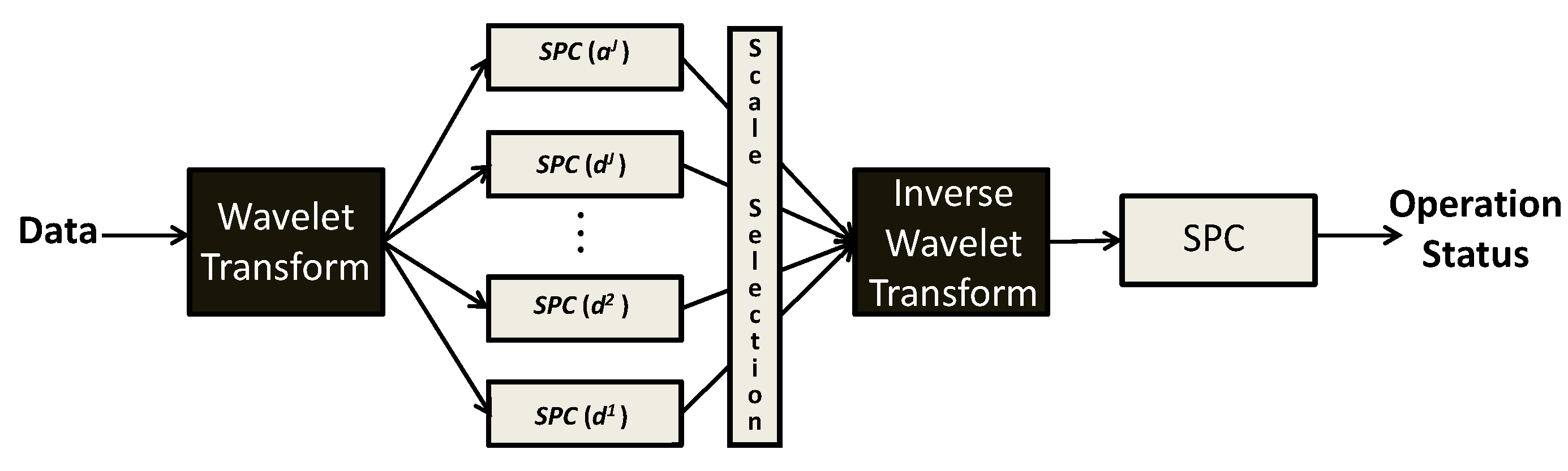
The energy compaction and decorrelation properties associated with the wavelet-based multiscale representation of data provide an adequate way for effectively detecting undesirable events with a wide range of time/frequency location and localization patterns, as well as to incorporate the natural complexity of the underlying phenomena in the normal operating conditions (NOC) models for process monitoring. Therefore, a considerable number of approaches have been developed to explore such potential [22]. Addressing univariate SPC (USPC), Top and Bakshi [49] proposed the idea of following the trends of wavelet coefficients at different scales using separate control charts. The state of the process is confirmed by reconstructing the signal back to the time domain, using only those coefficients from scales where control limits were exceeded, and checking against a detection limit calculated from such scales (where significant events were detected). This approach is called multiscale SPC (Figure 6). The approximate decorrelation ability of the wavelet transform makes this approach suitable even for autocorrelated processes, the signal power spectrum being accommodated by the scale-dependent nature of the statistical limits. Furthermore, energy compaction enables the effective detection and extraction of underlying deterministic events—fault signatures. The multiscale nature of this framework lead the authors to point out that it unifies Shewhart [50], CUSUM [51] and EWMA [52] procedures, as these control charts essentially differ in the scale at which data is represented [23].

Regarding multivariate applications, Kosanovich and Piovoso [53] presented an approach where the Haar wavelet transform coefficients obtained from filtered data (more specifically, after processing raw data with a finite impulse response median hybrid filter) were used for estimating a PCA model, which was finally applied for monitoring purposes. However, it was with Bakshi [54] that the first structured multivariate and multiscale SPC methodology was established. It was based on multiscale principal component analysis (MSPCA), which combines the wavelet transform ability to approximately decorrelate autocorrelated processes (and extract abnormal faulty patterns in the signals), together with the PCA ability to model the variables’ correlation structure. A theoretical analysis of the properties underlying multivariate and multiscale statistical process control (MSSPC) can be found in [55]. Several other works report improvements or modifications made to the original base formulation [56,57,58,59,60] and a variety of applications of multiscale methods to process monitoring have been reported since then [61,62,63,64,65,66,67,68,69,70,71,72,73,74,75,76,77,78], including for the more complex case of batch processes [79,80]. More recently, image-based monitoring methods [81,82] were developed as well as methods dedicated to supervision of slowly evolving degradation phenomena, closely related to prognosis of equipment health and reliability [78,83,84].

2.3. Multiscale Methods for Predictive Modelling

Multiscale methods have been developed for parametric as well as non-parametric predictive modelling. Applications in parametric regression analysis usually involve compression of the predictor space when it presents serial redundancy; i.e., when there is a functional relationship linking the values from successive variables—for instance, when they are relative to wavelengths from digitized spectra, a common situation in multivariate calibration. By eliminating components with low predictive power, it is possible to reduce the variability of predictions [85,86,87,88,89] and build more parsimonious and stable models [85,90,91]. Several strategies were proposed for selecting the number of transformed predictors (i.e., wavelet coefficients) to include in the model, such as those based upon the variance spectra of the coefficients, where the coefficients with the largest variances are selected [90], leave-one-out cross-validation [86], root mean square error (RMS), truncation of elements in the PLS weight vector, followed by re-orthogonalization, and mutual information [85].

2.4. Multiscale Methods for System Identification and Optimal Estimation

There are several different ways by which multiscale methods can be used for system identification and their application scenarios range from time-invariant systems [92,93] to non-linear black-box modelling, e.g., in the identification of Hammerstein model structures [94] or in neural networks, as activation functions [95,96,97,98,99,100,101].

Noticing that all standard linear-in-parameter system identification methods can be understood as projections onto a given basis set, Carrier and Stephanopoulos [102] applied wavelets basis sets in order to develop a system identification procedure with improved performance in estimating reduced-order models and non-linear systems, as well as systems corrupted with noise and disturbances, by focusing on the open-loop cross-over frequency region. Plavajjhala, et al. [103] used wavelet-based prefilters for system identification, proposing the parameter estimates computed at the scale (frequency band) at which the signal-to-noise ratio is maximal. The use of wavelets as basis functions is also adopted by Tsatsanis and Giannakis [104] in the identification of time-varying systems, and a similar approach was followed by Doroslovački and Fan [105] for adaptive filtering purposes, with the robustness issues being treated elsewhere [106].

Nikolaou et al. presented a methodology for estimating finite impulse response models (FIR) by compressing the Kernel (sequence of coefficients in the FIR model) using a wavelet expansion [107], and applied the same reasoning to nonlinear model structures; namely, to quadratic discrete Volterra models [108].

On the other hand, Dijkerman and Mazumdar [109] analyzed the correlation structure of the wavelet coefficients computed for several stochastic processes (see also Tewfik [110]), and proposed multiresolution stochastic models as approximations to these original processes, motivated by the tree-based models presented elsewhere [111].

Regarding multiscale optimal estimation, Chui and Chen [112] implemented an on-line Kalman filtering approach that estimates the wavelet coefficients at each scale, and claimed evidence that it conducts to improve performance over the classical way of implementing it, when applied to a Brownian random walk process. Renaud, et al. [113] also proposed a procedure for multiscale autoregressive time series prediction, based on the redundant à trous wavelet transform (non-decimated Haar filter bank), and developed a filtering scheme that takes advantage of such a decomposition, which is similar to Kalman filtering. A multiscale Kalman filtering approach based on scale-dependent models, can be found in [114]. This approach performs Kalman filtering in the scales where a dynamical model can reliably be estimated and wavelet thresholding in the others that are dominated by unstructured stochastic stationary noise. A related platform for multiscale system identification can be found in [115].

Applications of wavelets have also been proposed in the related field of time-series analyses; namely for: estimation of parameters that define long range dependency [38,116,117,118]; analysis of 1/f processes [38,119,120], including fractional Brownian motion [121,122,123,124] as well the detection of 1/f noise in the presence of analytical signals [125]; scale-wise decomposition of the sample variance of a time series (wavelet-based analysis of variance; see [38]); analysis of electrochemical noise measurements in corrosion processes [126]; and analysis of acoustic emission signals in dense-phase pneumatic transport for identifying regimes and a variety of flow phenomena [127].

2.5. Multiscale Methods for Data Denoising

De-noising concerns uncovering the true signal from noisy data where it is immersed, and is one of the application fields where multiscale methods have found wide application. The success arises mainly from their ability to concentrate deterministic features of the signal in a few high magnitude wavelet coefficients while the energy associated with stochastic phenomena is spread over all coefficients. This property is instrumental for the implementation of thresholding strategies in the wavelet domain. Donoho and Johnstone pioneered the field and proposed a simple and effective de-noising scheme for estimating a signal with additive i.i.d. zero-mean Gaussian white noise [128]. This scheme is called “VisuShrink”, since it provides better visual quality than other procedures based on mean-squared-error alone. This is an example of a non-linear estimation procedure, since wavelet thresholding is both adaptive and signal dependent, in opposition to what happens, for instance, with the optimal linear Wiener filtering [33] or with thresholding policies that tacitly eliminate all the high frequency coefficients, sometimes also known as smoothing techniques [43,87].

Since publication of the pioneering work by Donoho and Johnstone, there have been numerous contributions regarding modifications and extensions to the base procedure, in order to improve denoising performance. For instance, orthogonal wavelet transforms lack the translation-invariant property and this often causes the appearance of artifacts (also known as pseudo-Gibbs phenomena) in the neighborhood of discontinuities. Coifman and Donoho proposed a translation invariant procedure that essentially consists of averaging out several de-noised versions of the signal (using orthogonal wavelets), obtained for several shifts, after un-shifting [129]. In simple terms, the procedure consists of performing the sequence of operations “Average [Shift—De-noise—Unshift]”, a scheme called “Cycle Spinning” by Coifman. With such a procedure, not only the pseudo-Gibbs phenomenon near the vicinities of discontinuities are greatly reduced, but also the results are often so good that lower sampling rates can be employed.

The judicious choice of a proper thresholding criterion was also the target of various contributions, and several alternative approaches have been proposed, such as those based on cross-validation [130], minimum description length [131], minimization of Bayes risk [132], and on level-adaptive Bayesian modelling in the wavelet domain [133]. More elaborate discussions regarding this topic can be found elsewhere [134,135]. The simultaneous choice of the decomposition level and/or wavelet filter was addressed by Pasti, et al. [136] and Tewfik, et al. [137].

Image de-noising does not encompass any fundamental difference from 1D signal de-noising, apart from the fact that a 2D wavelet transform is now required. The computation of the 2D wavelet transform can be implemented by successively applying 1D orthogonal wavelets to the rows and columns of the matrix of pixel intensities, in an alternate fashion, implicitly giving rise to separable 2D wavelet basis (tensor products of the 1D basis functions); non-separable 2D wavelet functions are also available [33,41,135] and can be used for this (or other) purpose.

The approaches referred above consist of implementing de-noising schemes through off-line data processing. Within the scope of on-line data rectification, where the goal is also the accommodation of errors present in measurements in order to improve data quality for carrying out other tasks such as process control, process monitoring, and fault diagnosis, Nounou and Bakshi [138] proposed a multiscale approach for situations where no knowledge regarding the underlying process model is available. It basically consists of implementing the classical denoising algorithm with a boundary corrected filter in a sliding window of dyadic length, retaining only the last point of the reconstructed signal for online use (OnLine Multiscale rectification, OLMS). When there is some degree of correlation between the different variables acquired, Bakshi, et al. [139] presented a methodology where PCA is used to build up an empirical model for handling such redundancies. Finally, for the situation where knowledge about the systems structure is sufficient to postulate a linear dynamical state-space model for the finest scale behavior, a multiscale data rectification approach was also proposed, using a Bayesian error-in-variables (EIV) formalism [140].

3. Multi-Granularity Methods

Multi-granularity methods (also called multiresolution methods) address the challenge of handling the coexistence of data with different granularities or levels of aggregation, i.e., with different resolutions (not to be confounded with the Metrology concept with the same name). Therefore, they are primarily a response to the demand imposed by modern data acquisition technologies that create multi-granularity data structures in order to keep up with the data flood—data is being aggregated in summary statistics or features, instead of storing every collected observation. But, as will be explored below, multi-granularity methods can also be applied to improve the quality of the analysis, even when raw data is all at the same resolution. By selectively introducing granularity in each variable (if necessary), it is possible to optimize and significantly improve the performance of, for instance, predictive models (see more on Section 3.2).

The usual tacit assumption for data analysis is that all available records have the same resolution or granularity, usually considered to be concentrated around the sampling instants (which should, furthermore, be equally spaced). Analyzing modern process databases, one can easily verify that this assumption is frequently not met. It is rather common to have data collectors taking data from the process pointwisely; i.e., instantaneously, at a certain rate, while quality variables often result from compound sampling procedures, i.e., material is collected during some predefined time, after which the resulting volume is mixed and submitted to analysis; the final value represents a low resolution measurement of the quality attribute with a time granularity corresponding to the material collection period. Still other variables can be stored as averages over hours, shifts, customer orders, or production batches, resulting from numerical operations implemented in the process Distributed Control Systems (DCS) or by operators. Therefore, modern databases present, in general, a Multiresolution data structure, and this situation will tend to be found with increasing incidence as Industry 4.0 takes its course.

Multiresolution structures require the use of dedicated modelling and processing tools that effectively deal with the multiresolution character and optimally merge multiple sources of information with different granularities. However, this problem has been greatly overlooked in the literature. Below, we refer to some of the efforts undertaken to explicitly incorporate the multiresolution structure of data in the analysis or, alternatively (but also highly relevant and opportune), to take advantage of introducing it (even if it is no there initially), for optimizing the analysis performance.

3.1. Multi-Granularity Methods for Process Monitoring

An example, perhaps isolated, of a process monitoring approach developed for handling simultaneously the complex multivariate and multiscale nature of systems and the existence of multiresolution data collected from them, was proposed by Reis and Saraiva [141]: MR-MSSPC. Similarly to MSSPC [54,56], this methodology implements scale-dependent multivariate statistical process control charts on the wavelet coefficients (fault detection and feature extraction stage), followed by a second confirmatory stage that is triggered if any event is detected at some scale during the first stage. However, the composition of the multivariate models available at each scale depends on the granularity of data collected and is not the same for all of them, as happened in MSSPC. This implies algorithmic differences in the two stages as well as on the receding horizon windows used to implement the method online. This results in a clearer definition of the regions where abnormal events take place and a more sensitive response when the process is brought back to normal operation. MR-MSSPC brings out the importance of distinguishing between multiresolution (multi-granularity) and multiscale concepts: MSSPC is a multiscale, single-resolution approach, whereas MR-MSSPC is a multiscale, multiresolution methodology.

3.2. Multi-Granularity Modelling and Optimal Estimation

Willsky et al. developed, in a series of works, the theory for Multiresolution Markov models, which could then be applied to signal and image processing applications [142,143,144]. This class of models share a similar structure to the classical state-space formulation, but they are defined over the scale domain, rather than the time domain. These allow data analyses over multiple resolutions (granularity levels), which is the fundamental requirement for implementing optimal fusion schemes for images with different resolutions such as satellite and ground images. In this regard, Multiresolution Markov models were developed for addressing multiresolution problems in space (e.g., image fusion). However, they do not apply when the granularity concerns time. In this case, new model structures are required that should be flexible enough to accommodate for measurements with different granularities. In the scope of multiresolution soft sensors (MR-SS) for industrial applications, Rato and Reis [145] proposed a scalable model structure with such multi-granularity capability embedded—the scalability arises from its estimability in the presence of many variables, eventually highly correlated (a feature inherited from Partial Least Squares, PLS, which is estimation principle adopted). The use of a model structure (MR-SS) that is fully consistent with the multiresolution data structure leads to: (i) an increase in model interpretability (the modelling elements regarding multiresolution and dynamic aspects are clearly identified and accommodated); (ii) higher prediction power (due to the use of more parsimonious and accurate models); (iii) paves the way to the development of advanced signal processing tools; namely, optimal multiresolution Kalman filters [111,144,146,147].

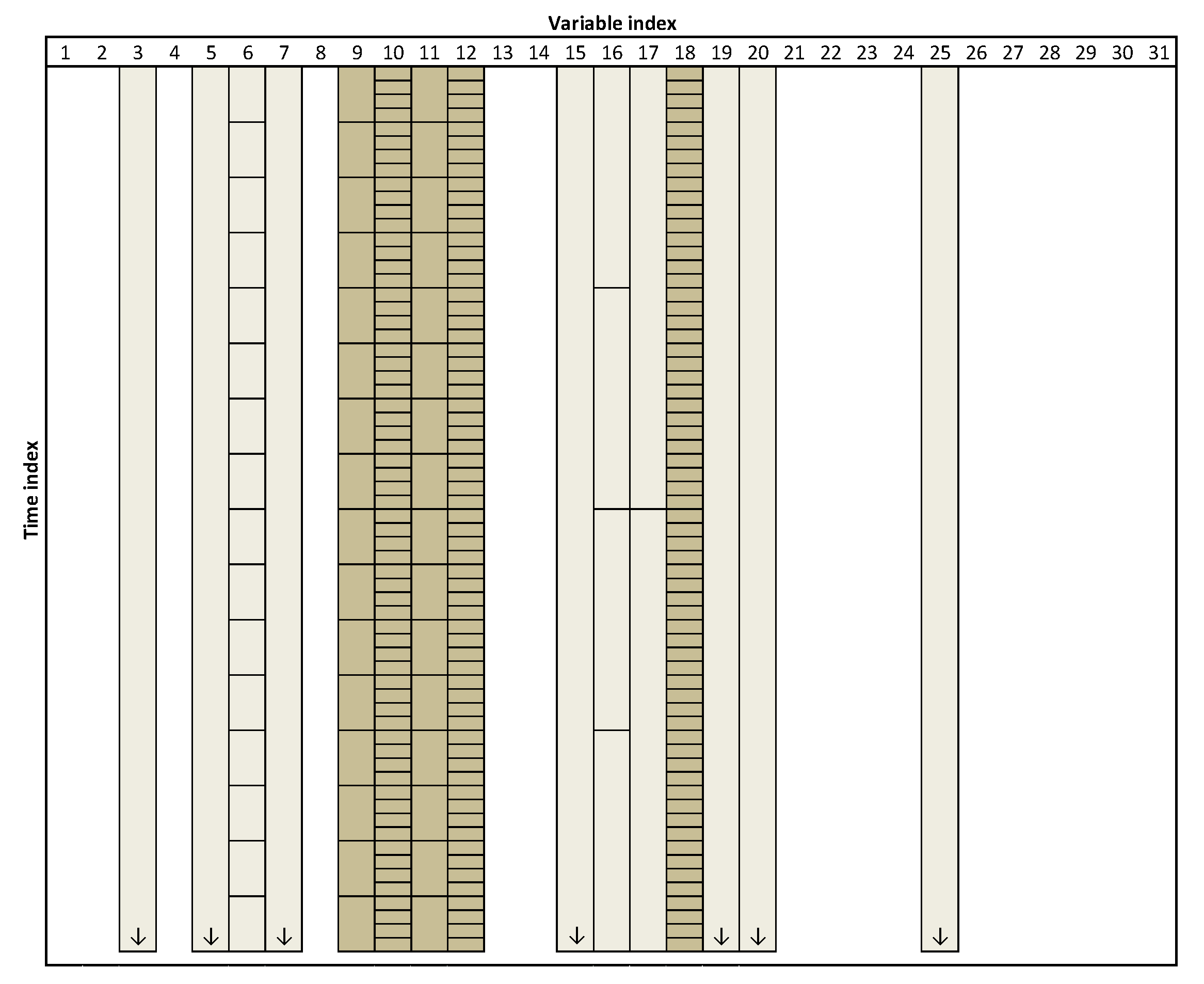
But there is another motivation for being interested in multiresolution analysis besides the need to handle it when present in data—even when the data is available at a single-resolution (i.e., all variables have the same granularity), there is no guarantee whatsoever that this native resolution is the most appropriate for analysis. On the contrary, there are reasons to believe the opposite, as this choice is usually made during the commissioning of the IT infrastructure, long before engineers or data analysts (or even someone connected to the operation or management of the process) become involved in the development of data-driven models. Therefore, it should be in the best interest of the analyst to have the capability of tuning the optimal granularity to use for each variable, in order to maximize the quality of the outputs of data analysis. The optimal selection of variables’ resolution or granularity has been implemented with significant success for developing inferential models for quality attributes in both batch [148] as well as continuous processes [149]. Notably, it can be theoretically guaranteed that the derived multiresolution models perform at least as well as their conventional single-resolution counterparts. For the sake of illustration, in a case study with real data, the improvement in predictive performance achieved was of 54% [148]. Figure 7 presents a scheme highlighting the set of variables selected in this case study, to estimate the target response (polymer viscosity) and the associated optimal resolution at which they should be represented.

3.3. Multiresolution Projection Frameworks for Industrial Data

The computation of approximations at different resolutions can be done in a variety of ways. Using wavelet-based frameworks is one of them, but the resulting approximation sequence present granularities following a dyadic progression, i.e., where the degree of delocalization doubles when moving from one resolution level to the next. But the time-granularity may also be flexibly imposed by the user, according to the nature of the task or decision to be made. In this case, one must abandon the classic wavelet-based framework, and work on averaging operators that essentially perform the same actions on the raw signals as wavelet approximation (or low-pass) filters do. These averaging operations can also be interpreted as projections to approximation subspaces, as in the wavelet multiresolution construct, but now these subspaces are more flexibly obtained and do not have to conform to the rigid structure imposed in the wavelet framework.

One problem multiresolution frameworks have to deal with when processing industrial data, is missing data. This is an aspect that wavelet multiresolution projections cannot handle by default, and the same applies to conventional averaging operators. One solution found to this prevalent problem (all industrial databases have many instances of missing data, with different patterns and origins) can be found in the scope of uncertainty-based projection methods [150]. In this setting, each data record is represented by a value and the associated uncertainty. Values correspond to measurements, whereas the uncertainty is a “parameter, associated with the result of a measurement, that characterizes the dispersion of the values that could reasonably be attributed to the measurand” [151]. According to the “Guide to the Expression of Uncertainty in Measurement” (GUM) the standard uncertainty, $u(x_i)$ (to which we will refer here simply as uncertainty), is expressed in terms of a standard deviation of the values collected from a series of observations (the so called Type A evaluation), or through other adequate means (Type B evaluation), namely, relying upon an assumed probability density function expressing a degree of belief. With the development of sensors and metrology, both quantities are now routinely available and their simultaneous use is actively promoted and even enforced by standardization organizations. Classical data analysis tasks, formerly based strictly on raw data, such as Principal Components Analysis and Multivariate Linear Regression approaches (e.g., Ordinary Least Squares, Principal Components Regression) are also being upgraded to their uncertainty-based counterparts, that explicitly consider combined data/uncertainty structures [152,153,154,155,156,157]. The same applies to multiresolution frameworks where the averaging operator may incorporate both aspects of data (measurements and their uncertainty), and, in this way directly address and solve, in an elegant way, the missing data problem: a missing value can be easily replaced by an estimate of it together the associated uncertainty. In the worst case, the historical mean can be imputed, having associated the historical standard deviation, but often more accurate missing data imputation methods can be adopted to perform this task [158,159,160,161]. Examples of multiresolution projection frameworks developed for handling missing data and heteroscedastic uncertainties in industrial settings can be found in [150].

4. Conclusions

As industrial processes evolve, new challenges emerge imposed by the increasing complexity of systems and data collected from them. Multiscale methods offer suitable frameworks to handle the former type of challenges (complexity), whereas multi-granularity methods are designed to address the issues raised by new data collectors. Multiscale methods operate in a transformed space where the scale parameter is explicitly incorporated in the mathematical formalism. This is the case of the wavelet transform, which constitute the backbone of mainstream data-driven multiscale methods. The wavelet transform is obtained by convolution operations with wavelet filters corresponding to the so called wavelet functions, or simply wavelets. Wavelets tile the entire time-frequency plane in a complete and very effective way [44,48,56,162,163,164], and therefore their coefficients (the wavelet transform) contain the fundamental information localized in these time-frequency regions. In this way, multiscale methods are able to zoom into the systems’ behavior taking place at different scales or frequency bands, thus enabling multiscale analysis.

On the other hand, data resolution is a key aspect of the Quality of Information extracted from empirical studies, as proposed in the InfoQ framework developed by Kenett and Shmueli [165,166]; see also [167]. Multi-granularity provides effective tools to increase the quality of information generated in data-driven analysis by properly handling multiresolution data structures or by optimally selecting the data granularity for a given purpose.

Small and medium-sized enterprises (SMEs) are often part of wider supply chains that are becoming increasingly integrated systems where information and materials flow in a complex way. The management and optimization of such networks will require a new analytics toolbox, able to deal with the existence of dynamics at multiple scales in time and space as well as the existence of data with different resolutions. The two categories of methods reviewed in this article have the potential to play an increasing role in industrial data science for SMEs (as well as for larger-sized companies). However, they are not yet part of the usual data science toolbox and therefore more research is required to extend existent solutions to make them more user friendly for the purpose of increasing their adoption. Targeted areas include: spectroscopic soft sensors development (where multi-granularity methods are showing very good performances); monitoring of multistage batch processes (where variables show different dynamical signatures, calling for the application of multiscale methods); and optimal time-aggregation of high throughput data-streams (e.g., for prediction purposes), among others.

References

- Qin, S.J. Process data Analytics in the Era of Big Data. AICHE J. 2014, 60, 3092–3100. [Google Scholar] [CrossRef]
- Reis, M.S.; Gins, G. Industrial Process Monitoring in the Big Data/Industry 4.0 Era: From Detection, to Diagnosis, to Prognosis. Processes 2017, 5, 35. [Google Scholar] [CrossRef]
- Reis, M.S.; Braatz, R.D.; Chiang, L.H. Big Data—Challenges and Future Research Directions. Chem. Eng. Prog. 2016, 46–50. [Google Scholar]
- Ge, Z.; Song, Z.; Gao, F. Review of Recent Research on Data-Based Process Monitoring. Ind. Eng. Chem. Res. 2013, 52, 3543–3562. [Google Scholar] [CrossRef]
- Li, D.; Shah, S.L.; Chen, T. Indentification of fast-rate models from multirate data. Int. J. Control 2001, 74, 680–689. [Google Scholar] [CrossRef]
- Lu, N.; Yang, Y.; Gao, F.; Wang, F. Multirate Dynamic Inferential Modeling for Multivariable Processes. Chem. Eng. Sci. 2004, 59, 855–864. [Google Scholar] [CrossRef]
- Wang, J.; Chen, T.; Huang, B. Multirate sample-data systems: Computing fast-rate models. J. Process Control 2004, 14, 79–88. [Google Scholar] [CrossRef]
- Xie, L.; Yang, H.; Huang, B. FIR model identification of multirate processes with random delays using EM algorithm. AICHE J. 2013, 59, 4124–4132. [Google Scholar] [CrossRef]
- Wu, Y.; Luo, X. A novel calibration approach of soft sensor based on multirate data fusion technology. J. Process Control 2010, 20, 1252–1260. [Google Scholar] [CrossRef]
- Shang, C.; Huang, X.; Suykens, J.A.K.; Huang, D. Enhancing dynamic soft sensors based on DPLS: A temporal smoothness regularization approach. J. Process Control 2015, 28, 17–26. [Google Scholar] [CrossRef]
- Li, W.; Shah, S.L.; Xiao, D. Kalman filters in non-uniformly sampled multirate systems: For FDI and beyond. Automatica 2008, 44, 199–208. [Google Scholar] [CrossRef]
- Fatehi, A.; Huang, B. Kalman filtering approach to multi-rate information fusion in the presence of irregular sampling date and variable measurement delay. J. Process Control 2017, 53, 15–25. [Google Scholar] [CrossRef]
- Izadi, I.; Zhao, Q.; Chen, T. An Optimal Scheme for Fast Rate Fault Detection Based on Multirate Sampled Data. J. Process Control 2005, 15, 307–319. [Google Scholar] [CrossRef]
- Cong, Y.; Ge, Z.; Song, Z. Multirate Partial Least Squares for Process Monitoring. In Proceedings of the 9th IFAC Symposium on Advanced Control of Chemical Processes ADCHEM 2015, Whistler, BC, Canada, 7–10 June 2015; pp. 771–776. [Google Scholar]
- Birol, I.; Ündey, C.; Birol, G.; Çinar, A. PenSim: A Web-Based Simulator for Penicillin Production. Int. J. Eng. Simul. 2001, 2, 24–30. [Google Scholar]
- Tangirala, A.K.; Li, D.; Patwardhan, R.; Shah, S.L.; Chen, T. Issues in multirate process control. In Proceedings of the American Control Conference, San Diego, CA, USA, 2–4 June 1999. [Google Scholar]
- Braatz, R.D.; Alkire, R.C.; Rusli, E.; Drews, T.O. Multiscale Systems Engineering with Application to Chemical Reaction Processes. Chem. Eng. Sci. 2004, 59, 5623–5628. [Google Scholar] [CrossRef]
- Charpentier, J.-C. Perspective on multiscale methodology for product design and engineering. Comput. Chem. Eng. 2009, 33, 936–946. [Google Scholar] [CrossRef]
- Christofides, P.D.; Armaou, A.; Lou, Y.; Varshney, A. Control and Optimization of Multiscale Process Systems; Birkhäuser: Basel, Switzerland, 2009. [Google Scholar]
- Kwon, J.S.-I.; Nayhouse, M.; Christofides, P.D. Multiscale, Multidomain Modeling and Parallel Computation: Application to Crystal Shape Evolution in Crystallization. Ind. Eng. Chem. Res. 2015, 54, 11903–11914. [Google Scholar] [CrossRef]
- Li, M.; Christofides, P.D. Multi-Scale Modeling and Analysis of an Industrial HVOF Thermal Spray Process. Chem. Eng. Sci. 2005, 60, 3649–3669. [Google Scholar] [CrossRef]
- Ganesan, R.; Das, T.K.; Venkataraman, V. Wavelet Based Multiscale Process Monitoring—A Literature Review. IIE Trans. Qual. Reliab. Eng. 2004, 36, 787–806. [Google Scholar] [CrossRef]
- Bakshi, B.R. Multiscale Analysis and Modeling Using Wavelets. J. Chemom. 1999, 13, 415–434. [Google Scholar] [CrossRef]
- Reis, M.S.; Saraiva, P.M. Multivariate and Multiscale Data Analysis. In Statistical Practice in Business and Industry; Coleman, S., Greenfield, T., Stewardson, D., Montgomery, D.C., Eds.; Wiley: Chichester, UK, 2008; pp. 337–370. [Google Scholar]
- Grasso, M.; Colosimo, B.M. An Automated Approach to Enhance Multiscale Signal Monitoring of Manufacturing Processes. J. Manuf. Sci. Eng. 2016, 138, 051003. [Google Scholar] [CrossRef]
- Huang, N.E.; Shen, S.S.P. (Eds.) Hilbert-Huang Transform and Its Applications; World Scientific Publishing Co.: Singapore, 2005; Volume 5. [Google Scholar]
- Du, Y.; Du, D. Fault detection and diagnosis using empirical mode decomposition based principal component analysis. Comput. Chem. Eng. 2018, 115, 1–21. [Google Scholar] [CrossRef]
- Hubbard, B.B. The World According to Wavelets—The Story of a Mathematical Technique in the Making, 2nd ed.; A K Peters: Natick, MA, USA, 1998. [Google Scholar]
- Walker, J.S. A Primer on Wavelets and Their Scientific Applications; Chapman & Hall/CRC: Boca Raton, FL, USA, 1999. [Google Scholar]
- Burrus, C.S.; Gopinath, R.A.; Guo, H. Introduction to Wavelets and Wavelet Transforms—A Primer; Prentice Hall: Upper Saddle River, NJ, USA, 1998. [Google Scholar]
- Aboufadel, E.; Schlicker, S. Discovering Wavelets; Wiley: New York, NY, USA, 1999. [Google Scholar]
- Chan, Y.T. Wavelet Basics; Kluwer: Boston, MA, USA, 1995. [Google Scholar]
- Mallat, S. A Wavelet Tour of Signal Processing; Academic Press: San Diego, CA, USA, 1998. [Google Scholar]
- Strang, G.; Nguyen, T. Wavelets and Filter Banks; Wellesley-Cambridge Press: Wellesley, MA, USA, 1997. [Google Scholar]
- Kaiser, G. A Friendly Guide to Wavelets; Birkhäuser: Boston, MA, USA, 1994. [Google Scholar]
- Walter, G.G. Wavelets and Other Orthogonal Systems with Applications; CRC Press: Boca Raton, FL, USA, 1994. [Google Scholar]
- Chui, C.K. An Introduction to Wavelets; Academic Press: San Diego, CA, USA, 1992. [Google Scholar]
- Percival, D.B.; Walden, A.T. Wavelets Methods for Time Series Analysis; Cambridge University Press: Cambridge, UK, 2000. [Google Scholar]
- Cohen, A.; Ryan, R.D. Wavelets and Multiscale Signal Processing; Chapman & Hall: London, UK, 1995. [Google Scholar]
- Starck, J.-L.; Murtagh, F.; Bijaoui, A. Image Processing and Data Analysis—The Multiscale Approach; Cambridge University Press: Cambridge, UK, 1998. [Google Scholar]
- Vetterli, M.; Kovačević, J. Wavelets and Subband Coding; Prentice Hall: Upper Sadle River, NJ, USA, 1995. [Google Scholar]
- Motard, R.L.; Joseph, B. (Eds.) Wavelet Applications in Chemical Engineering; Kluwer: Boston, MA, USA, 1994. [Google Scholar]
- Chau, F.-T.; Liang, Y.-Z.; Gao, J.; Shao, X.-G. Chemometrics—From Basics to Wavelet Transform; Wiley: Hoboken, NJ, USA, 2004; Volume 164. [Google Scholar]
- Daubechies, I. Ten Lectures on Wavelets; SIAM: Philadelphia, PA, USA, 1992; Volume 61. [Google Scholar]
- Alsberg, B.K.; Woodward, A.M.; Kell, D.B. An Introduction to Wavelet Transforms for Chemometricians: A Time-Frequency Approach. Chemom. Intel. Lab. Syst. 1997, 37, 215–239. [Google Scholar] [CrossRef]
- Rioul, O.; Vetterli, M. Wavelets and Signal Processing. IEEE Signal Process. Mag. 1991, 8, 14–38. [Google Scholar] [CrossRef]
- Kreyszig, E. Introductory Functional Analysis with Applications; Wiley: New York, NY, USA, 1978. [Google Scholar]
- Mallat, S. A Theory for Multiresolution Signal Decomposition: The Wavelet Representation. IEEE Trans. Pattern Anal. Mach. Intell. 1989, 11, 674–693. [Google Scholar] [CrossRef]
- Top, S.; Bakshi, B.R. Improved Statistical Process Control Using Wavelets. In Proceedings of the Foundation of Computer Aided Process Operations FOCAPO 98, Snowbird, UT, USA, 5–10 July 1998; pp. 332–337. [Google Scholar]
- Shewhart, W.A. Economic Control of Quality of Manufactured Product; D. Van Nostrand Company, Inc.: New York, NY, USA, 1931; Republished in 1980 as a 50th Anniversary Commemorative Reissue by ASQC Quality Press, Milwaukee, WI, USA. [Google Scholar]
- Page, E.S. Continuous Inspection Schemes. Biometrics 1954, 41, 100–115. [Google Scholar] [CrossRef]
- Roberts, S.W. Control Charts Tests Based on Geometric Moving Averages. Technometrics 1959, 1, 239–250. [Google Scholar] [CrossRef]
- Kosanovich, K.A.; Piovoso, M.J. PCA of Wavelet Transformed Process Data for Monitoring. Intell. Data Anal. 1997, 1, 85–99. [Google Scholar] [CrossRef]
- Bakshi, B.R. Multiscale PCA with Application to Multivariate Statistical Process Control. AICHE J. 1998, 44, 1596–1610. [Google Scholar] [CrossRef]
- Aradhye, H.B.; Bakshi, B.R.; Strauss, R.; Davis, J.F. Multiscale SPC Using Wavelets: Theoretical Analysis and Properties. AICHE J. 2003, 49, 939–958. [Google Scholar] [CrossRef]
- Reis, M.S.; Bakshi, B.R.; Saraiva, P.M. Multiscale statistical process control using wavelet packets. AICHE J. 2008, 54, 2366–2378. [Google Scholar] [CrossRef] [Green Version]
- Kano, M.; Nagao, K.; Hasebe, S.; Hashimoto, I.; Ohno, H.; Strauss, R.; Bakshi, B.R. Comparison of Multivariate Statistical Process Monitoring Methods with Applications to the Eastman Challenge Problem. Comput. Chem. Eng. 2002, 26, 161–174. [Google Scholar] [CrossRef]
- Misra, M.; Yue, H.H.; Qin, S.J.; Ling, C. Multivariate Process Monitoring and Fault Diagnosis by Multi-Scale PCA. Comput. Chem. Eng. 2002, 26, 1281–1293. [Google Scholar] [CrossRef]
- Yoon, S.; MacGregor, J.F. Unifying PCA and Multiscale Approaches to Fault Detection and Isolation. In Proceedings of the 6th IFAC Symposium on Dynamics and Control of Process Systems, Jejudo Island, Korea, 4–6 June 2001. [Google Scholar]
- Yoon, S.; MacGregor, J.F. Principal-Component Analysis of Multiscale Data for Process Monitoring and Fault Diagnosis. AICHE J. 2004, 50, 2891–2903. [Google Scholar] [CrossRef]
- Aradhye, H.B.; Bakshi, B.R.; Davis, J.F.; Ahalt, S.C. Clustering in Wavelet Domain: A Multiresolution ART Network for Anomaly Detection. AICHE J. 2004, 50, 2455–2466. [Google Scholar] [CrossRef]
- Aradhye, H.B.; Davis, J.F.; Bakshi, B.R. ART-2 and Multiscale ART-2 for On-Line Process Fault Detetction—Validation Via Industrial Case Studies and Monte Carlo Simulation. Annu. Rev. Control 2002, 26, 113–127. [Google Scholar] [CrossRef]
- Zhao, J.; Chen, B.; Schen, J. Multidimensional Non-Orthogonal Wavelet-Sigmoid Basis Function Neural Network for Dynamic Process Fault Diagnosis. Comput. Chem. Eng. 1998, 23, 83–92. [Google Scholar] [CrossRef]
- Luo, R.; Misra, M.; Himmelblau, D.M. Sensor Fault Detection via Multiscale Analysis and Dynamic PCA. Ind. Eng. Chem. Res. 1999, 38, 1489–1495. [Google Scholar] [CrossRef]
- Bakhtazad, A.; Palazoglu, A.; Romagnoli, J.A. Detection and Classification of Abnormal Process Situations Using Multidimensional Wavelet Domain Hidden Markov Trees. Comput. Chem. Eng. 2000, 24, 769–775. [Google Scholar] [CrossRef]
- Sun, W.; Palazoğlu, A.; Romagnoli, J.A. Detecting Abnormal Process Trends by Wavelet-Domain Hidden Markov Models. AICHE J. 2003, 49, 140–150. [Google Scholar] [CrossRef]
- Tsuge, Y.; Hiratsuka, K.; Takeda, K.; Matsuyama, H. A Fault Detection and Diagnosis for the Continuous Process with Load-Fluctuations Using Orthogonal Wavelets. Comput. Chem. Eng. 2000, 24, 761–767. [Google Scholar] [CrossRef]
- Daiguji, M.; Kudo, O.; Wada, T. Application of Wavelet Analysis to Fault Detection in Oil Refinery. Comput. Chem. Eng. 1997, 21, S1117–S1122. [Google Scholar] [CrossRef]
- Jiang, T.; Chen, B.; He, X. Industrial Application of Wavelet Transform to the On-Line Prediction of Side Draw Qualities of Crude Unity. Comput. Chem. Eng. 2000, 24, 507–512. [Google Scholar] [CrossRef]
- Alexander, S.M.; Gor, T.B. Monitoring, Diagnosis and Control of Industrial Processes. Comput. Ind. Eng. 1998, 35, 193–196. [Google Scholar] [CrossRef]
- Jiao, X.J.; Davies, M.S.; Dumont, G.A. Wavelet Packet Analysis of Paper Machine Data for Control Assessment and Trim Loss Optimization. Pulp Pap. Can. 2004, 105, 34–37. [Google Scholar]
- Watson, G.H.; Gilholm, K.; Jones, J.G. A Wavelet-Based Method for Finding Inputs of Given Energy which Maximize the Outputs of Nonlinear Systems. Int. J. Syst. Sci. 1999, 30, 1297–1307. [Google Scholar] [CrossRef]
- Lada, E.K.; Lu, J.-C.; Wilson, J.R. A Wavelet-Based Procedure for Process Fault Detection. IEEE Trans. Semicond. Manuf. 2002, 15, 79–90. [Google Scholar] [CrossRef]
- Jin, J.; Shi, J. Feature-Preserving Data Compression of Stamping Tonnage Information Using Wavelets. Technometrics 1999, 41, 327–339. [Google Scholar] [CrossRef]
- Jin, L.; Shi, J. Automatic Feature Extraction of Waveform Signals for In-Process Diagnostic Peformance Improvement. J. Intell. Manuf. 2001, 12, 257–268. [Google Scholar] [CrossRef]
- Jeong, M.K.; Lu, J.-C.; Huo, X.; Vidakovic, B.; Chen, D. Wavelet-Based Data Reduction Techniques for Process Fault Detection; Georgia Institute of Technology, School of Industrial and Systems Engineering, Statistics Group: Atlanta, GA, USA, 2004. [Google Scholar]
- Naghooai, E.; Huang, B. Wavelet Transform Based Methodology for Detection and Characterization of Multiple Oscillations in Nonstationary Variables. Ind. Eng. Chem. Res. 2017, 56, 2083–2093. [Google Scholar] [CrossRef]
- He, Y.J.; Shen, J.N.; Shen, J.F.; Ma, Z.F. State of health estimation of lithium-ion batteries: A multiscale Gaussian process regression modeling approach. AICHE J. 2015, 61, 1589–1600. [Google Scholar] [CrossRef]
- Alawi, A.; Zhang, J.; Morris, J. Multiscale Multiblock Batch Monitoring: Sensor and Process Drift and Degradation. Org. Process Res. Dev. 2015, 19, 145–157. [Google Scholar] [CrossRef]
- Wang, J.; Qiu, K.; Liu, W.; Yu, T.; Zhao, L. Unsupervised-Multiscale-Sequential-Partitioning and Multiple-SVDD-Model-Based Process-Monitoring Method for Multiphase Batch Processes. Ind. Eng. Chem. Res. 2018, 57, 17437–17451. [Google Scholar] [CrossRef]
- Reis, M.S. An integrated multiscale and multivariate image analysis framework for process monitoring of colour random textures: MSMIA. Chemom. Intell. Lab. Syst. 2015, 142, 36–48. [Google Scholar] [CrossRef]
- Reis, M.S.; Bauer, A. Wavelet texture analysis of on-line acquired images for paper formation assessment and monitoring. Chemom. Intell. Lab. Syst. 2009, 95, 129–137. [Google Scholar] [CrossRef] [Green Version]
- Mounce, S.R.; Gaffney, J.W.; Boult, S.; Boxall, J.B. Automated Data-Driven Approaches to Evaluating and Interpreting Water Quality Time Series Data from Water Distribution Systems. J. Water Resour. Plan. Manag. 2015, 141, 04015026. [Google Scholar] [CrossRef] [Green Version]
- Xu, D.; Sui, S.B.; Zhang, W.; Xing, M.L.; Chen, Y.; Kang, R. RUL prediction of electronic controller based on multiscale characteristic analysis. Mech. Syst. Signal Process. 2018, 113, 253–270. [Google Scholar] [CrossRef]
- Alsberg, B.K.; Woodward, A.M.; Winson, M.K.; Rowland, J.J.; Kell, D.B. Variable Selection in Wavelet Regression Models. Anal. Chim. Acta 1998, 368, 29–44. [Google Scholar] [CrossRef]
- Cocchi, M.; Seeber, R.; Ulrici, A. Multivariate Calibration of Analytical Signals by WILMA (Wavelet Interface to Linear Modelling Analysis). J. Chemom. 2003, 17, 512–527. [Google Scholar] [CrossRef]
- Depczynsky, U.; Jetter, K.; Molt, K.; Niemöller, A. The Fast Wavelet Transform on Compact Intervals as a Tool in Chemometrics—II. Boundary Effects, Denoising and Compression. Chemom. Intell. Lab. Syst. 1999, 49, 151–161. [Google Scholar] [CrossRef]
- Jouan-Rimbaud, D.; Walczak, B.; Poppi, R.J.; de Noord, O.E.; Massart, D.L. Application of Wavelet Transform to Extract the Relevant Component from Spectral Data for Multivariate Calibration. Anal. Chem. 1997, 69, 4317–4323. [Google Scholar] [CrossRef] [PubMed]
- Eriksson, L.; Trygg, J.; Johansson, E.; Bro, R.; Wold, S. Orthogonal Signal Correction, Wavelet Analysis, and Multivariate Calibration of Complicated Process Fluorescence Data. Anal. Chim. Acta 2000, 420, 181–195. [Google Scholar] [CrossRef]
- Trygg, J.; Wold, S. PLS Regression on Wavelet Compressed NIR Spectra. Chemom. Intell. Lab. Syst. 1998, 42, 209–220. [Google Scholar] [CrossRef]
- Trygg, J. Parsimonious Multivariate Models. Ph.D. Thesis, Umeå University, Umeå, Sweden, 2001. [Google Scholar]
- Kosanovich, K.A.; Moser, A.R.; Piovoso, M.J. Poisson Wavelets Applied to Model Identification. J. Process Control 1995, 5, 225–234. [Google Scholar] [CrossRef]
- Pati, Y.C.; Rezaiifar, R.; Krishnaprasad, P.S.; Dayawansa, W.P. A Fast Recursive Algorithm for System Identification and Model Reduction Using Rational Wavelets. In Proceedings of the 27th Annual Asilomar Conference on Signals Systems and Computers, Pacific Grove, CA, USA, 1–3 November 1993. [Google Scholar]
- Hasiewicz, Z. Hammerstein System Identification by the Haar Multiresolution Approximation. Int. J. Adapt. Control Signal Process. 1999, 13, 691–717. [Google Scholar] [CrossRef]
- Bakshi, B.R.; Stephanopoulos, G. Wave-Net: A Multiresolution, Hierarchical Neural Network with Localized Learning. AICHE J. 1993, 39, 57–81. [Google Scholar] [CrossRef]
- Zhang, Q.; Benveniste, A. Wavelet Networks. IEEE Trans. Neural Netw. 1992, 3, 889–898. [Google Scholar] [CrossRef] [PubMed]
- Bakshi, B.R.; Koulouris, A.; Stephanopoulos, G. Learning at Multiple Resolutions: Wavelets as Basis Functions in Artificial Neural Networks and Inductive Decision Trees. In Wavelet Applications in Chemical Engineering; Kluwer Academic Publishers: Boston, MA, USA, 1994; pp. 139–174. [Google Scholar]
- Juditsky, A.; Zhang, Q.; Delyon, B.; Glorennec, P.-Y.; Benveniste, A. Wavelets in Identification—Wavelets, Splines, Neurons, Fuzzies: How Good for Identification? 2315; INRIA: Villers-lès-Nancy, France, 1994. [Google Scholar]
- Sjöberg, J.; Zhang, Q.; Ljung, L.; Benveniste, A.; Delyon, B.; Glorennec, P.-Y.; Hjalmarsson, H.; Juditsky, A. Nonlinear Black-box Modeling in System Identification: A Unified Overview. Automatica 1995, 31, 1691–1724. [Google Scholar] [CrossRef]
- Pati, Y.C.; Krishnaprasad, P.S. Analysis and Synthesis of Feedforward Neural Networks Using Discrete Affine Wavelet Transformations. IEEE Trans. Neural Netw. 1993, 4, 73–85. [Google Scholar] [CrossRef]
- Shi, B.; Yang, X.; Yan, L.X. Optimization of a crude distillation unit using a combination of wavelet neural network and line-up competition algorithm. Chin. J. Chem. Eng. 2017, 25, 1013–1021. [Google Scholar] [CrossRef]
- Carrier, J.; Stephanopoulos, G. Wavelet-Based Modulation in Control-Relevant Process Identification. AICHE J. 1998, 44, 341–360. [Google Scholar] [CrossRef]
- Plavajjhala, S.; Motard, R.L.; Joseph, B. Process Identification Using Discrete Wavelet Transforms: Design of Prefilters. AICHE J. 1996, 42, 777–790. [Google Scholar] [CrossRef]
- Tsatsanis, M.K.; Giannakis, G.B. Time-Varying System Identification and Model Validation Using Wavelets. IEEE Trans. Signal Process. 1993, 41, 3512–3523. [Google Scholar] [CrossRef]
- Doroslovački, M.I.; Fan, H. Wavelet-Based Linear System Modeling and Adaptative Filtering. IEEE Trans. Signal Process. 1996, 44, 1156–1167. [Google Scholar] [CrossRef]
- Doroslovački, M.I.; Fan, H.; Yao, L. Wavelet-Based Identification of Linear Discrete-Time Systems: Robustness Issue. Automatica 1998, 34, 1627–1640. [Google Scholar] [CrossRef]
- Nikolaou, M.; Vuthandam, P. FIR Model Identification: Parsimony Through Kernel Compression with Wavelets. AICHE J. 1998, 44, 141–150. [Google Scholar] [CrossRef]
- Nikolaou, M.; Mantha, D. Efficient Nonlinear Modeling Using Wavelets and Related Compression Techniques. In Proceedings of the NSF Workshop on Nonlinear Model Predictive Control, Ascona, Switzerland, 2–6 June 1998. [Google Scholar]
- Dijkerman, R.W.; Mazumdar, R.R. Wavelet Representations of Stochastic Processes and Multiresolution Stochastic Models. IEEE Trans. Signal Process. 1994, 42, 1640–1652. [Google Scholar] [CrossRef]
- Tewfik, A.H. Correlation Structure of the Discrete Wavelet Coefficients of Fractional Brownian Motion. IEEE Trans. Inf. Theory 1992, 38, 904–909. [Google Scholar] [CrossRef]
- Bassevile, M.; Benveniste, A.; Chou, K.C.; Golden, S.A.; Nikoukhah, R.; Willsky, A.S. Modeling and Estimation of Multiresolution Stochastic Processes. IEEE Trans. Inf. Theory 1992, 38, 766–784. [Google Scholar] [CrossRef]
- Chui, C.K.; Chen, G. Kalman Filtering with Real-Time Applications, 3rd ed.; Springer: Berlin, Germany, 1999; Volume 17. [Google Scholar]
- Renaud, O.; Starck, J.-L.; Murtagh, F. Wavelet-Based Combined Signal Filtering and Prediction. IEEE Trans. Syst. Man Cibern. Part B 2005, 35, 1241–1251. Available online: http://www.unige.ch/~renaud/papers/abstractKalmanWavelet.html (accessed on 22 January 2019). [CrossRef] [Green Version]
- Rendall, R.R.; Reis, M.S. A Comparison Study of Single-Scale and Multiscale Approaches for Data-Driven and Model-Based Online Denoising. Qual. Reliab. Eng. Int. 2014, 30, 935–950. [Google Scholar] [CrossRef]
- Reis, M.S. A Multiscale Empirical Modeling Framework for System Identification. J. Process Control 2009, 19, 1546–1557. [Google Scholar] [CrossRef]
- Abry, P.; Veitch, D.; Flandrin, P. Long-Range Dependence: Revisiting Aggregation with Wavelets. J. Time Ser. Anal. 1998, 19, 253–266. [Google Scholar] [CrossRef]
- Veitch, D.; Abry, P. A Wavelet-Based Joint Estimator of the Parameters of Long-Range Dependence. IEEE Trans. Inf. Theory 1999, 45, 878–897. [Google Scholar] [CrossRef]
- Whitcher, B. Wavelet-Based Estimation for Seasonal Long-Memory Processes. Technometrics 2004, 46, 225–238. [Google Scholar] [CrossRef] [Green Version]
- Wornell, G.W. A Karhunen-Loève-like Expansion for 1/f Processes via Wavelets. IEEE Trans. Inf. Theory 1990, 36, 859–861. [Google Scholar] [CrossRef]
- Wornell, G.W.; Oppenheim, A.V. Estimation of Fractal Signals from Noisy Measurements Using Wavelets. IEEE Trans. Signal Process. 1992, 40, 611–623. [Google Scholar] [CrossRef]
- Flandrin, P. Wavelet Analysis and Synthesis of Fractional Brownian Motion. IEEE Trans. Inf. Theory 1992, 38, 910–917. [Google Scholar] [CrossRef]
- Ramanathan, J.; Zeitouni, O. On the Wavelet Transform of Fractional Brownian Motion. IEEE Trans. Inf. Theory 1991, 37, 1156–1158. [Google Scholar] [CrossRef]
- Flandrin, P. On the Spectrum of Fractional Brownian Motion. IEEE Trans. Inf. Theory 1989, 35, 197–199. [Google Scholar] [CrossRef]
- Masry, E. The Wavelet Transform of Stochastic Processes with Stationary Increments and Its Application to Fractional Brownian Motion. IEEE Trans. Inf. Theory 1993, 39, 260–264. [Google Scholar] [CrossRef]
- Mittermayr, C.R.; Lendl, B.; Rosenberg, E.; Grasserbauer, M. The Application of the Wavelet Power Spectrum to Detect and Estimate 1/f Noise in the Presence of Analytical Signals. Anal. Chim. Acta 1999, 388, 303–313. [Google Scholar] [CrossRef]
- Wharton, J.A.; Wood, R.J.K.; Mellor, B.G. Wavelet Analysis of Electrochemical Noise Measurements During Corrosion of Austenitic and Superduplex Stainless Steels in Chloride Media. Corros. Sci. 2003, 45, 97–122. [Google Scholar] [CrossRef]
- He, L.L.; Yang, Y.; Huang, Z.L.; Liao, Z.W.; Wang, J.D.; Yang, Y.R. Multi-Scale Analysis of Acoustic Emission Signals in Dense-Phase Pneumatic Conveying of Pulverized Coal at High Pressure. AICHE J. 2016, 62, 2635–2648. [Google Scholar] [CrossRef]
- Donoho, D.L.; Johnstone, I.M. Ideal Spatial Adaptation by Wavelet Shrinkage; Department of Statistics, Stanford University: Stanford, CA, USA, 1992. [Google Scholar]
- Coifman, R.R.; Donoho, D.L. Translation-Invariant De-Noising; Department of Statistics, Stanford University: Stanford, CA, USA, 1995. [Google Scholar]
- Nason, G.P. Wavelet Shrinkage Using Cross-Validation. J. R. Stat. Soc. Ser. B 1996, 58, 463–479. [Google Scholar] [CrossRef]
- Cohen, I.; Raz, S.; Malah, D. Translation-Invariant Denoising Using the Minimum Description Length Criterion. Signal Process. 1999, 75, 201–223. [Google Scholar] [CrossRef]
- Ruggeri, F.; Vidakovic, B. A Baysean Decision Theoretic Approach to the Choice of Thresholding Parameter. Stat. Sin. 1999, 9, 183–197. [Google Scholar]
- Vidakovic, B.; Ruggeri, F. BAMS Method: Theory and Simulations. Sankhyā Indian J. Stat. 2001, 63, 234–249. [Google Scholar]
- Nason, G.P. Choice of the Threshold Parameter in Wavelet Function Estimation. In Wavelets and Statistics; Antoniadis, A., Oppenheim, G., Eds.; Springer-Verlag: New York, NY, USA, 1995; pp. 261–299. [Google Scholar]
- Jansen, M. Noise Reduction by Wavelet Thresholding; Springer: New York, NY, USA, 2001; Volume 161. [Google Scholar]
- Pasti, L.; Walczak, B.; Massart, D.L.; Reschiglian, P. Optimization of Signal Denoising in Discrete Wavelet Transform. Chemom. Intell. Lab. Syst. 1999, 48, 21–34. [Google Scholar] [CrossRef]
- Tewfik, A.H.; Sinha, D.; Jorgensen, P. On the Optimal Choise of a Wavelet for Signal Representation. IEEE Trans. Inf. Theory 1992, 38, 747–765. [Google Scholar] [CrossRef]
- Nounou, M.N.; Bakshi, B.R. On-Line Multiscale Filtering of Random and Gross Errors Without Process Models. AICHE J. 1999, 45, 1041–1058. [Google Scholar] [CrossRef]
- Bakshi, B.R.; Bansal, P.; Nounou, M.N. Multiscale Rectification of Random Errors Without Process Models. Comput. Chem. Eng. 1997, 21, S1167–S1172. [Google Scholar] [CrossRef]
- Ungarala, S.; Bakshi, B.R. A Multiscale, Baysean and Error-In-Variables Approach for Linear Dynamic Data Rectification. Comput. Chem. Eng. 2000, 24, 445–451. [Google Scholar] [CrossRef]
- Reis, M.S.; Saraiva, P.M. Multiscale Statistical Process Control with Multiresolution Data. AICHE J. 2006, 52, 2107–2119. [Google Scholar] [CrossRef]
- Bassevile, M.; Benveniste, A.; Willsky, A.S. Multiscale Autoregressive Processes, Part I: Schur-Levinson Parametrizations. IEEE Trans. Signal Process. 1992, 40, 1915–1934. [Google Scholar] [CrossRef]
- Bassevile, M.; Benveniste, A.; Willsky, A.S. Multiscale Autoregressive Processes, Part II: Lattice Structures for Whitening and Modeling. IEEE Trans. Signal Process. 1992, 40, 1935–1954. [Google Scholar] [CrossRef]
- Willsky, A.S. Multiresolution Markov Models for Signal and Image Processing. Proc. IEEE 2002, 90, 1396–1458. [Google Scholar] [CrossRef]
- Rato, T.J.; Reis, M.S. Multiresolution Soft Sensors (MR-SS): A New Class of Model Structures for Handling Multiresolution Data. Ind. Eng. Chem. Res. 2017, 56, 3640–3654. [Google Scholar] [CrossRef]
- Chou, K.C.; Willsky, A.S.; Benveniste, A. Multiscale Recursive Estimation, Data Fusion, and Regularization. IEEE Trans. Autom. Control 1994, 39, 464–478. [Google Scholar] [CrossRef]
- Chou, K.C.; Willsky, A.S.; Nikoukhah, R. Multiscale Systems, Kalman Filters, and Riccati Equations. IEEE Trans. Autom. Control 1994, 39, 479–492. [Google Scholar] [CrossRef]
- Geert, G.; Van Impe, J.F.M.; Reis, M.S. Finding the optimal time resolution for batch-end quality prediction: MRQP—A framework for Multi-Resolution Quality Prediction. Chemom. Intell. Lab. Syst. 2018, 172, 150–158. [Google Scholar]
- Rato, T.J.; Reis, M.S. Building Optimal Multiresolution Soft Sensors for Continuous Processes. Ind. Eng. Chem. Res. 2018, 57, 9750–9765. [Google Scholar] [CrossRef]
- Reis, M.S.; Saraiva, P.M. Generalized Multiresolution Decomposition Frameworks for the Analysis of Industrial Data with Uncertainty and Missing Values. Ind. Eng. Chem. Res. 2006, 45, 6330–6338. [Google Scholar] [CrossRef]
- BIPM; IEC; IFCC; ISO; IUPAC; IUPAP; OIML. Guide to the Expression of Uncertainty; ISO: Geneva, Switzerland, 1993. [Google Scholar]
- Bro, R.; Sidiropoulos, N.D.; Smilde, A.K. Maximum Likelihood Fitting Using Ordinary Least Squares Algorithms. J. Chemom. 2002, 16, 387–400. [Google Scholar] [CrossRef]
- Reis, M.S.; Saraiva, P.M. Integration of Data Uncertainty in Linear Regression and Process Optimization. AICHE J. 2005, 51, 3007–3019. [Google Scholar] [CrossRef]
- Río, F.J.; Rio, J.; Rius, F.X. Prediction Intervals in Linear Regression Taking into Account Errors in Both Axis. J. Chemom. 2001, 15, 773–788. [Google Scholar]
- Wentzell, P.D.; Andrews, D.T.; Hamilton, D.C.; Faber, K.; Kowalski, B.R. Maximum Likelihood Principal Component Analysis. J. Chemom. 1997, 11, 339–366. [Google Scholar] [CrossRef]
- Wentzell, P.D.; Andrews, D.T.; Kowalski, B.R. Maximum Likelihood Multivariate Calibration. Anal. Chem. 1997, 69, 2299–2311. [Google Scholar] [CrossRef]
- Wentzell, P.D.; Lohnes, M.T. Maximum Likelihood Principal Component Analysis with Correlated Measurements Errors: Theoretical and Practical Considerations. Chemom. Intell. Lab. Syst. 1999, 45, 65–85. [Google Scholar] [CrossRef]
- Arteaga, F.; Ferrer, A. Dealing with Missing Data in MSPC: Several Methods, Different Interpretations, Some Examples. J. Chemom. 2002, 16, 408–418. [Google Scholar] [CrossRef]
- Little, R.J.A.; Rubin, D.B. Statistical Analysis with Missing Data, 2nd ed.; Wiley: Hoboken, NJ, USA, 2002. [Google Scholar]
- Nelson, P.R.C.; Taylor, P.A.; MacGregor, J.F. Missing Data Methods in PCA and PLS: Score Calculations with Incomplete Observations. Chemom. Intell. Lab. Syst. 1996, 35, 45–65. [Google Scholar] [CrossRef]
- Walczak, B.; Massart, D.L. Dealing with Missing Data. Chemom. Intell. Lab. Syst. 2001, 58, 15–27, 29–42. [Google Scholar] [CrossRef]
- Bruce, A.; Donoho, D.; Gao, H.-Y. Wavelet Analysis. IEEE Spectr. 1996, 33, 26–35. [Google Scholar] [CrossRef]
- Mallat, S. A Wavelet Tour of Signal Processing, 2nd ed.; Academic Press: San Diego, CA, USA, 1999. [Google Scholar]
- Reis, M.S.; Bakshi, B.R.; Saraiva, P.M. Denoising and Signal to Noise Enhancement: Wavelet Transform and Fourier Transform. In Comprehensive Chemometrics: Chemical and Biochemical Data Analysis; Brown, S., Tauler, R., Walczak, B., Eds.; Elsevier: Oxford, UK, 2009; Volume 2, pp. 25–55. [Google Scholar]
- Kenett, R.S.; Shmueli, G. On Information Quality. J. R. Stat. Soc. A 2014, 177, 3–38. [Google Scholar] [CrossRef]
- Kenett, R.S.; Shmueli, G. Information Quality: The Potential of Data and Analytics to Generate Knowledge; Wiley: New York, NY, USA, 2016. [Google Scholar]
- Reis, M.S.; Kenett, R.S. Assessing the Value of Information of Data-Centric Activities in the Chemical Processing Industry 4.0. AICHE J. 2018, 64, 3868–3881. [Google Scholar] [CrossRef]
Figure 1.
The complementary deductive and inductive branches of Process Systems Engineering (PSE) 4.0.
Figure 2.
An artificial signal containing multiscale features: a linear trend, a sinusoid, a step perturbation, a spike (deterministic features with different frequency localization characteristics) and white noise (a stochastic feature whose energy is uniformly distributed in the time/frequency plane).
Figure 3.
Schematic illustration of the time/frequency windows associated with the basis function for the following linear transforms: (a) Dirac-δ transform, (b) Fourier transform and (c) windowed Fourier transform.
Figure 4.
Schematic representation of the tiling of the time-frequency plane provided by the wavelet basis functions (“Heisenberg boxes”) (a), and an illustration of how wavelets divide the frequency domain (b), where it is possible to verify that they essentially work as a set of bandpass filters. The shape of the windows and frequency bands, for a given wavelet function, depend upon the scale index value: for low values of the scale index, the windows have good time localizations and cover a long frequency band; for high values of the scale index, the time coverage is broader and the degree of frequency localization is higher (more concentration is a narrower frequency region).
Figure 5.
The signal in Figure 2 decomposed into its coarser version at scale plus all the details lost across the scales ranging from to . The filter used here is the Daubechies’s compactly supported filter with 3 vanishing moments (A wavelet has p vanishing moments if for . This is an important property in the fields of signal and image compression, since it can induce a higher number of low magnitude detail coefficients, if the signal does have local regularity characteristics.).
Figure 6.
Scheme for the implementation of Multiscale Statistical Process Control.
Figure 7.
Schematic representation of the variables/resolutions selected for building the model. The size of the boxes represent the adopted granularity for each variable; the lighter shades indicate variable/resolutions that were pre-selected by the algorithm but discarded afterwards; the final combination of variables/resolution used in the model are represented with a darker color).
© 2019 by the author. Licensee MDPI, Basel, Switzerland. This article is an open access article distributed under the terms and conditions of the Creative Commons Attribution (CC BY) license (http://creativecommons.org/licenses/by/4.0/).
Share and Cite
MDPI and ACS Style
Reis, M.S. Multiscale and Multi-Granularity Process Analytics: A Review. Processes 2019, 7, 61. https://doi.org/10.3390/pr7020061
AMA Style
Reis MS. Multiscale and Multi-Granularity Process Analytics: A Review. Processes. 2019; 7(2):61. https://doi.org/10.3390/pr7020061
Chicago/Turabian StyleReis, Marco S. 2019. "Multiscale and Multi-Granularity Process Analytics: A Review" Processes 7, no. 2: 61. https://doi.org/10.3390/pr7020061
Note that from the first issue of 2016, this journal uses article numbers instead of page numbers. See further details here.