Geometric Modeling of Novel Generalized Hybrid Trigonometric Bézier-Like Curve with Shape Parameters and Its Applications

Abstract

The main objective of this paper is to construct the various shapes and font designing of curves and to describe the curvature by using parametric and geometric continuity constraints of generalized hybrid trigonometric Bézier (GHT-Bézier) curves. The GHT-Bernstein basis functions and Bézier curve with shape parameters are presented. The parametric and geometric continuity constraints for GHT-Bézier curves are constructed. The curvature continuity provides a guarantee of smoothness geometrically between curve segments. Furthermore, we present the curvature junction of complex figures and also compare it with the curvature of the classical Bézier curve and some other applications by using the proposed GHT-Bézier curves. This approach is one of the pivotal parts of construction, which is basically due to the existence of continuity conditions and different shape parameters that permit the curve to change easily and be more flexible without altering its control points. Therefore, by adjusting the values of shape parameters, the curve still preserve its characteristics and geometrical configuration. These modeling examples illustrate that our method can be easily performed, and it can also provide us an alternative strong strategy for the modeling of complex figures.

1. Introduction

Mathematical modeling, construction of curves and surfaces, and shape preserving [1,2,3,4,5,6] are very significant areas of research in computer-aided geometric design, computer-aided manufacturing, and computer graphics. Traditional Bézier curves, which is formed by the classical Bernstein basis functions and control points, have many excellent properties like symmetry, terminal properties, partition of unity, non-negativity, linear precision, integral property, convex hull property, etc. We can easily construct any shape by using parametric and geometric continuity constraints of the classical Bézier curve, but its drawback is that we cannot modify and cannot make a small adjustment in the shape of the curves design without changing the control points. To overcome this problem, we move towards those basis functions that possess shape parameters that help us to make small modifications in the shape of the curves according to our chosen values of the shape parameters. These shape parameters do not affect the physical and geometrical configuration of the curves.

In [7], Hering defined $C^2$ and $C^3$ continuous Bézier and B-spline curves with their tangent polygons. He considered the planner segmented Bézier curves and B-spline curves to present their parametric and geometric continuities. Yan [8] presented a particular family of Bézier curves with three different shape parameters, which are also known as adjustable Bézier curves. Those curves have same shape and structure like the traditional quartic Bézier curve. Schneider et al. [9] described the discrete fairing of curves and surfaces, which is based on linear curvature distribution. In [10], geometric and parametric continuities with arc length parametrization and smoothness were presented. Here, the basic results of the geometric continuity of the curve were also discussed in a self-contained way. Hu et al. [11] presented the modeling of free-form complex curves by using geometric continuities of SG-Bézier (shape-adjustable generalized Bézier) curves and also presented their properties and applications. In [12], Bashir et al., presented the $C^2$ and $G^2$ continuity conditions with their applications by using the rational quadratic trigonometric Bézier curve. They also constructed a conic section-like circle and ellipse by using this rational quadratic trigonometric Bézier curve. Usman et al. [13] constructed a new trigonometric cubic Bézier-like curve for free-form complex curve modeling with some applications in engineering. Qin et al. gave the parametric and geometric continuity conditions of GE Bézier curves and also presented the geometric significance of shape parameters in [14].

In [15], BiBi et al. presented the modeling of symmetric curves and surfaces in the 2D and 3D plane. They developed a new technique for the modeling of symmetric figures, which is very useful in our daily life. Misro et al. [16] presented a new quintic trigonometric Bézier curve with two shape parameters. Its parametric, as well as curvature continuity were also discussed in this work. In [17], Veltkamp presented the survey of the parametric and geometric continuities of curves and surfaces and also established the visibility of continuities and graphic algorithms. Hu et al., developed a method for geometric continuity constraints and different modelings by using developable $\lambda$-Bézier surfaces in [18]. In [19,20,21], the modeling of different curves and surfaces by using B-spline curves and Bézier curves was presented. The techniques and algorithms were also discussed in these literature works. Sharma et al. [22] developed the shapes and modeling of the cubic trigonometric Bézier curve with two different shape parameters. In [23,24], the basis functions and their geometric and parametric continuities were presented. Moreover, the various modelings by different curves and surfaces were also presented here. Qin et al. [25] presented quartic trigonometric Bézier curves and also discussed their properties and presented their practical applications in the CAD/CAM field. In this research, the broad concept about geometric and solid modeling was also given. In [26], Han et al., presented the cubic trigonometric Bézier curve with two different shape parameters and its properties, and they also discussed the continuity constraints with the curve modeling. Hu et al., constructed the SG-Bézier curve with multiple shape parameters, and various modelings of engineering surfaces like swung surface, swept surface, rotation surface, etc., by the SG-Bézier basis were also discussed in [27]. In [28], Reenu Sharma constructed the quartic trigonometric Bézier (QTB) curve with two different shape parameters and discussed the properties of the QTB curve with shape modeling and the shape control of the curves.

Bashir et al. [29] designed various curves by the class of quasi-trigonometric Bézier curves having two shape parameters. Similarly, Yang et al. [30] also discussed the class of quasi-trigonometric Bézier curves. In [31], the quadratic trigonometric spline curve with multiple shape parameters was discussed, where each segment of the spline curve was obtained by four consecutive control points. The necessary and sufficient conditions were derived in [32] for introducing the separate Bézier part in order to represent some regular curves like the cycloid, etc. In [33], the rational Bézier model was generated by mixing polynomial and trigonometric functions. The shape preserving properties were also discussed in this work. Liang [34] introduced new Bernstein basis functions and Bézier curves with their properties. Liu et al. [35] presented a class of generalized Bézier curves and surfaces with multiple shape parameters. They also presented different modelings by using these Bézier curves and surfaces. In [36], a new formulation by the class of polynomial basis functions was presented for the construction of curves and surfaces. The properties of PHcurves in geometric modeling were presented in [37]. These PH curves could be computed at a speed similar to the polynomial curves. In [38], Wang et al. described the three conditions for the analysis of the curvature distribution. They also showed the significance of monotone curvature in CAGD/CAM. In [39], Yahya et al. presented the automatic generation of Arabic characters and font designing by using $G^1$ continuity conditions. A Bézier curve with shape parameters was presented by Wang in [40]. Furthermore, its significance and properties were also discussed in this work. In [41], Han et al., presented the shape analysis of the cubic trigonometric Bézier curve with its shape parameters and also its geometric significance and continuity conditions. Hu et al. [42] introduced Q-Bézier curves with their beneficial properties and shape adjustment with its multi-valued shape parameters. Pelosi et al., presented geometric Hermite interpolation depending on the orientation of the end tangents relative to the end point displacement vector in [43]. The problem of assigning tangents to a sequence of points compatible with a $G^1$ piecewise-PH-cubic spline interpolating of those points was also briefly addressed. Least squares approximation of Bézier coefficients with factored Hahn weights [44] provided the best constrained polynomial degree reduction with respect to the Jacobi $L2$-norm. This result afforded generalizations to many previous findings in the field of polynomial degree reduction. Various designs and models of $C^2$ algebraic-trigonometric Pythagorean hodograph splines with shape parameters were presented by González et al. [45]. Here, the curvature profile of some algebraic-trigonometric Pythagoreans was also presented.

This paper defines the curvature continuity of GHT-Bézier curves of order $n,(n\ge 2)$, which are described by taking a set of hybrid trigonometric Bernstein basis functions of degree two with three shape parameters, with identical characteristics to the classical Bernstein basis functions. In order to resolve the problem of not being able to construct complex curves using a single curve, we study the parametric and geometric continuity conditions for GHT-Bézier curves of degree n. Here, we join the various GHT-Bézier curves of the same/different degrees to obtain our required shape. Finally, the comparison of the curvature junction by GHT-Bézier curves and classical Bézier curves and some applications by different complex modelings (by using continuity conditions) are also presented.

In this work, we make the following technical contributions:

• $C^3$ continuity of the 2D GHT-Bézier curves.
• $G^k$ ($k\le 3$) geometric continuity of the 2D GHT-Bézier curves.
• a set of algorithms explaining how to enforce these constraints in practice.

This paper is organized into eight sections: In Section 2, the basic preliminaries and notations about the curvature, derivative of curvature, GHT-Bernstein basis functions, and the GHT-Bézier curve with its properties are discussed. In Section 3, the geometric significance of shape parameters and the relationship between the fixed point and GHT-Bézier curve are described. Similarly, the parametric and geometric continuity of GHT-Bézier curves with their mathematical and graphical results are given in Section 4. The comparison of the curvature junction of the GHT-Bézier curve and classical Bézier curve by $G^2$ and $G^3$ continuity with their valid results is presented in Section 5 and Section 6, respectively. Some applications of font designing and sketching by $C^3$ and $G^3$ continuity of GHT-Béezier curves are given in Section 7. Finally, a summarized conclusion is given in Section 8.

2. Preliminaries and Notations

We usually consider the Cartesian coordinate system to draw any curve. That is why we consider the control points in two tuples.

Similarly, boldface is used for points, as well as vectors. e.g.,

$$\mathbf{a}=\left(\begin{array}{c}{a}_x\\ a_y\end{array}\right)$$

and the Euclidean norm of a vector $\mathbf{a}$ can be defined as $\left|\right|\mathbf{a}\left|\right|=\sqrt{a_x^2+a_y^2},$ where $\mathbf{a}\left|\right|\mathbf{b}$ represents that the vectors $\mathbf{a}$ and $\mathbf{b}$ are parallel. The derivative of a function $f\left(\theta \right)$ can be represented as $f^{{}^{\prime }}\left(\theta \right).$

2.1. Curvature

In mathematics, curvature is a very strong concept of geometry. Basically, curvature is the amount by which any curve deviates about its position from being a straight line. For any parametric curve $S\left(\theta \right),$ the curvature with its mathematical expression can be written as follows,

$$\kappa \left(\theta \right)=\frac{S^{{}^{\prime }}\left(\theta \right)\times S^{{}^{″}}\left(\theta \right)}{\left|\right|S^{{}^{\prime }}\left(\theta \right){\left|\right|}^3}.$$

(1)

For any two-dimensional curve, its parametric equation can also be written as follows:

$$\kappa \left(\theta \right)=\frac{x^{{}^{\prime }}{y}^{{}^{″}}-y^{{}^{\prime }}{x}^{{}^{″}}}{{[{\left(x^{{}^{\prime }}\right)}^2+{\left(y^{{}^{\prime }}\right)}^2]}^{\frac{3}{2}}}.$$

(2)

In brief, the rate of change of curvature $\kappa \left(\theta \right)$ is defined by taking the first derivative of Equation (1), and we have:

$${\kappa }^{{}^{\prime }}\left(\theta \right)=\frac{\left|\right|S^{{}^{\prime }}\left(\theta \right){\left|\right|}^2\{S^{{}^{\prime }}\left(\theta \right)\times S^{{}^{‴}}\left(\theta \right)\}-3\{S^{{}^{\prime }}\left(\theta \right)\times S^{{}^{″}}\left(\theta \right)\}\{S^{{}^{\prime }}\left(\theta \right).S^{{}^{″}}\left(\theta \right)\}}{\left|\right|S^{{}^{\prime }}\left(\theta \right){\left|\right|}^5}$$

(3)

where $\left|\right|S^{{}^{\prime }}\left(\theta \right)\left|\right|$ is the magnitude of the tangent vector. Therefore, for any curvature, the radius of curvature is its reciprocal. By taking the first derivative of Equation (2), we obtain:

$${\kappa }^{{}^{\prime }}\left(\theta \right)=\frac{(x^{{}^{\prime }2}+y^{{}^{\prime }2})(x^{{}^{\prime }}{y}^{{}^{‴}}-y^{{}^{\prime }}{x}^{{}^{‴}})-3(x^{{}^{\prime }}{y}^{{}^{″}}-y^{{}^{\prime }}{x}^{{}^{″}})(x^{{}^{\prime }}{x}^{{}^{″}}+y^{{}^{\prime }}{y}^{{}^{″}})}{{({\left(x^{{}^{\prime }}\right)}^2+{\left(y^{{}^{\prime }}\right)}^2)}^{\frac{5}{2}}}$$

(4)

2.2. GHT-Bernstein Basis Functions of Degree n

Definition 1.

For any integer n, where $n=2$, the quadratic hybrid trigonometric (QHT) Bernstein basis functions in terms of variable $\theta \in [0,1]$ are defined as follows,

$$\left\{\begin{array}{c}{q}_{0,2}\left(\theta \right)=(1-sin\left(\frac{\pi }{2}\theta \right))(1-\nu sin\left(\frac{\pi }{2}\theta \right))e^{\gamma \theta }\hfill \\ q_{1,2}\left(\theta \right)=1-q_{0,2}\left(\theta \right)-q_{2,2}\left(\theta \right)\hfill \\ q_{2,2}\left(\theta \right)=(1-cos\left(\frac{\pi }{2}\theta \right))(1-\beta cos\left(\frac{\pi }{2}\theta \right))e^{(1-\gamma )\theta }.\hfill \end{array}\right.$$

For $n\ge 3$, the function $q_{i,n}\left(\theta \right)$ where $(i=0,1,2\dots .,n),$ is recursively defined by:

$$q_{i,n}\left(\theta \right)=(1-\theta )q_{i,n-1}\left(\theta \right)+\theta q_{i-1,n-1}\left(\theta \right)$$

(5)

and is known as GHT-Bernstein basis functions as in [15]. Moreover, the function $q_{i,n}\left(\theta \right)=0$ if and only if $i=-1$ or $i>n$ and $\nu ,\beta ,\gamma \in [-1,1]$ are the shape parameters defined in the given domain.

Remark 1.

It is noted that the expressions given in Definition 1 differ from the ones we introduced in our earlier work [15] in that we explicitly removed the λ parameter (i.e., λ is set to zero in the current paper). We found in our experiments that this parameter was not intuitive enough for the users to control, while resulting in unnecessarily complex computations. As we prove in this work, we were able to derive sufficiently high order derivative constraints (up to $C^3$ and $G^3$) while keeping this parameter set to zero. We advocate therefore Definition 1 from now on.

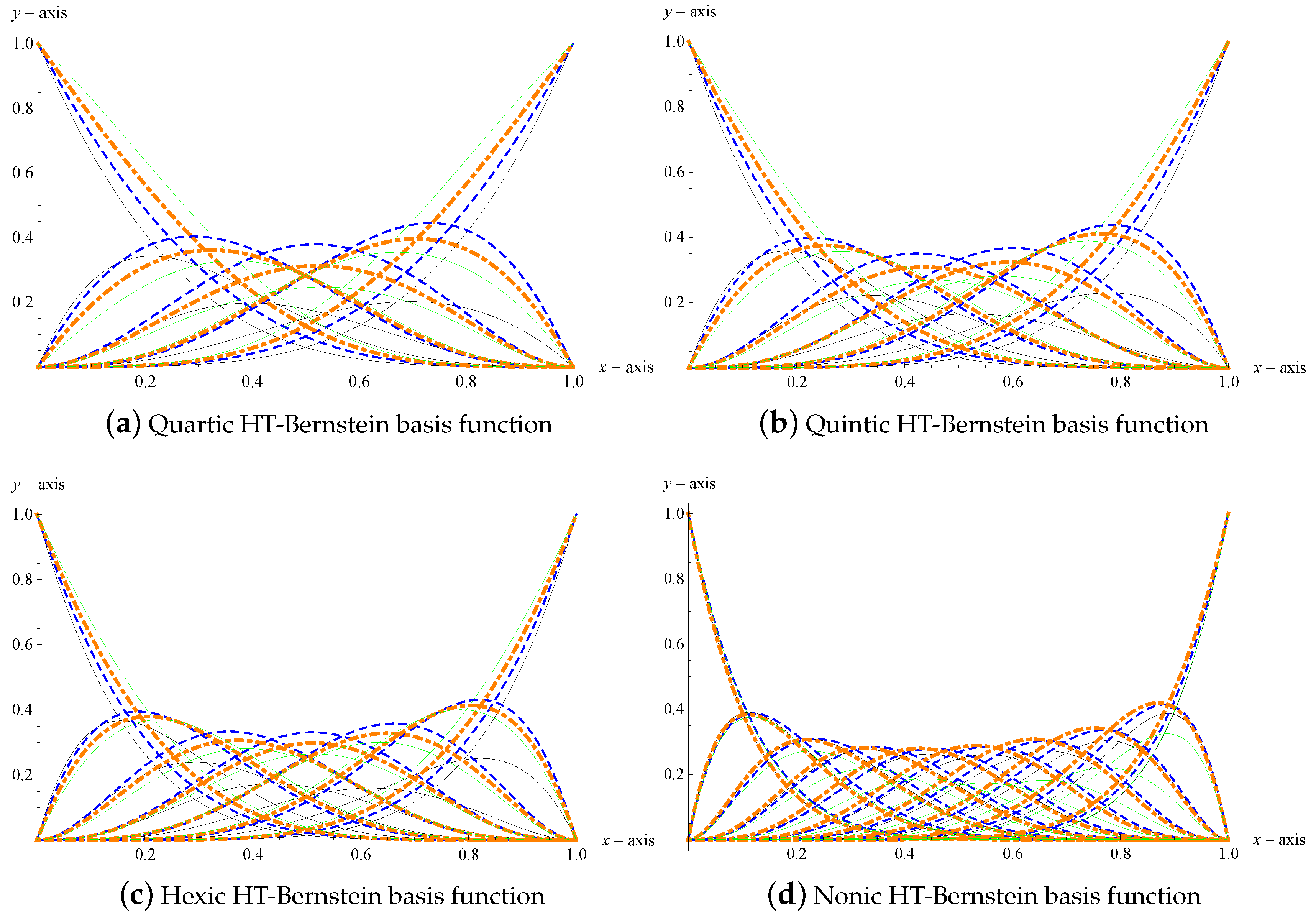
Figure 1 illustrates the graphs for GHT-Bernstein basis functions with different values of n and by the alteration of shape parameters. The black (solid), blue (dashed), orange (dash + dotted), and green (solid) lines were obtained by varying the values of shape parameters. These four figures also depict that the GHT-Bernstein basis functions gives us the same graphical representation as the traditional Bernstein basis functions. Therefore, they must possess all basic properties of traditional Bernstein basis functions.

Theorem 1.

The GHT-Bernstein basis functions have the basic properties like symmetry, positivity, partition of unity, and terminal properties.

1.

Partition of unity: The GHT-Bernstein basis functions satisfy the partition of unity, i.e.,

$$\sum _{i=0}^n{q}_{i,n}\left(\theta \right)=1.$$

2.

Positivity: In the given domain of shape parameters $\nu ,\beta$, and γ, the GHT-Bernstein basis functions are non-negative or $q_{i,n}\left(\theta \right)\ge 0$ for $i=0,1,2,3,\dots ,n.$

3.

Symmetry: For the fixed values of shape parameters $\nu =\beta =\gamma$, the function $q_{i,n}\left(\theta \right)$ where $(i=0,1,2,3,\dots ,n)$ is symmetric, i.e.,

$$q_{i,n}(\theta ,\nu ,\beta ,\gamma )=q_{n-i,n}(1-\theta ,\nu ,\beta ,\gamma ).$$

4.

End point interpolation property: For the shape parameters $\nu ,\beta ,\gamma$ and for given variable $\theta ,$ the function satisfies the end point interpolation properties as:

$$\left\{\begin{array}{c}{q}_{i,n}\left(0\right)=1,i=0\hfill \\ q_{i,n}\left(0\right)=0,i=1,2,3,\dots ,n\hfill \\ q_{n,n}\left(1\right)=1,i=n\hfill \\ q_{i,n}\left(1\right)=0,i=0,1,2,3,\dots ,n-1\hfill \end{array}\right.$$

(6)

and the first derivatives of these functions at their end points are:

$$\left\{\begin{array}{c}{q}_{i,n}^{\prime }\left(0\right)=\frac{1}{2}[-\pi (1+\nu )-2((n-2)-\gamma )],i=0\hfill \\ q_{i,n}^{\prime }\left(0\right)=(n-2)+\frac{1}{2}\pi (1+\nu )-\gamma ,i=1\hfill \\ q_{i,n}^{\prime }\left(0\right)=0,i=2,3,4,\dots ,n\hfill \\ q_{i,n}^{\prime }\left(1\right)=0,i=0,1,2,3,\dots ,n-2\hfill \\ q_{i,n}^{\prime }\left(1\right)=\frac{1}{2}[-\pi (1+\beta )-2((n-2)+\gamma )],i=n-1\hfill \\ q_{i,n}^{\prime }\left(1\right)=(n-2)+\frac{1}{2}\pi (1+\beta )-\gamma ,i=n.\hfill \end{array}\right.$$

(7)

Proof. 

The proof of the above results is as described in [15].  □

2.3. GHT-Bézier Curves of Degree n

Definition 2.

A class of parametric GHT-Bézier curves with the given set of control points $P_i^{*}$, where $(i=0,1,2,3,\dots ..,n)$ and shape parameters $\nu ,$ β, and γ are defined in Equation (8):

$$\left\{{\Pi }_{n,\theta }\right\}:S(\theta ;\nu ,\beta ,\gamma )=\sum _{i=0}^n{P}_i^{*}{q}_{i,n}\left(\theta \right),0\le \theta \le 1.$$

(8)

where $q_{i,n}\left(\theta \right)$ are called GHT-Bernstein basis functions.

Consider a cubic HT-Bézier curve with the control points $P_0^{*}=(0,0)$, $P_1^{*}=(2,1)$, $P_2^{*}=(3,0)$, and $P_3^{*}=(5,1)$ and shape parameters $\nu ,\beta$ and $\gamma$.

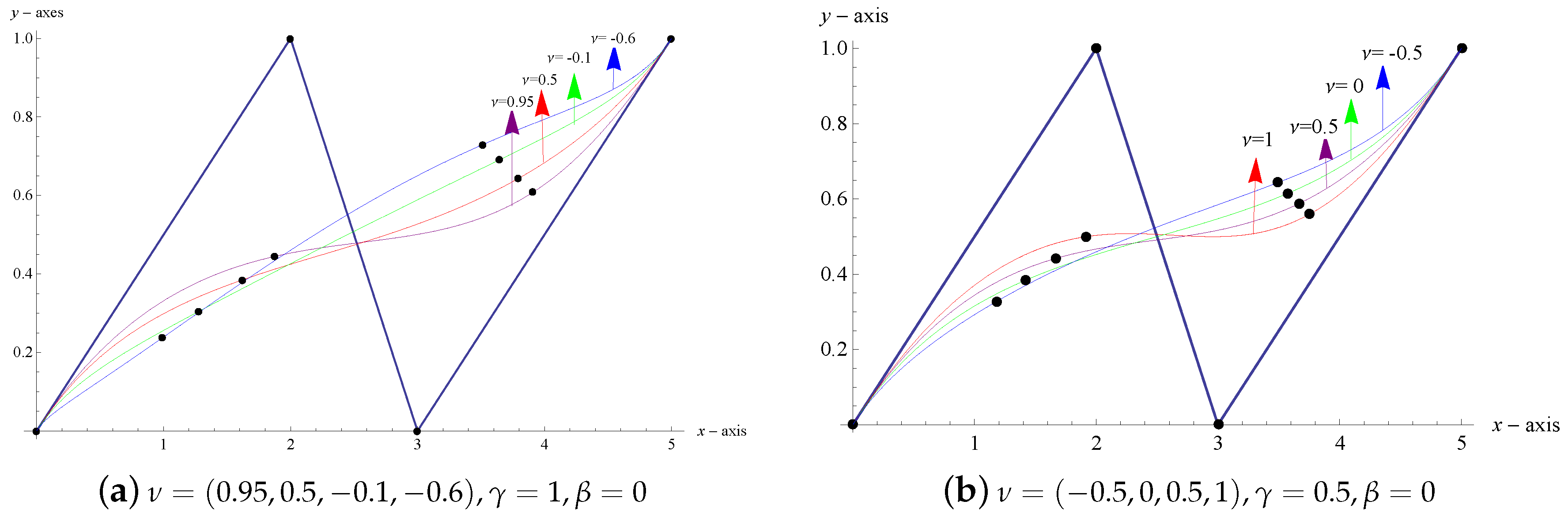
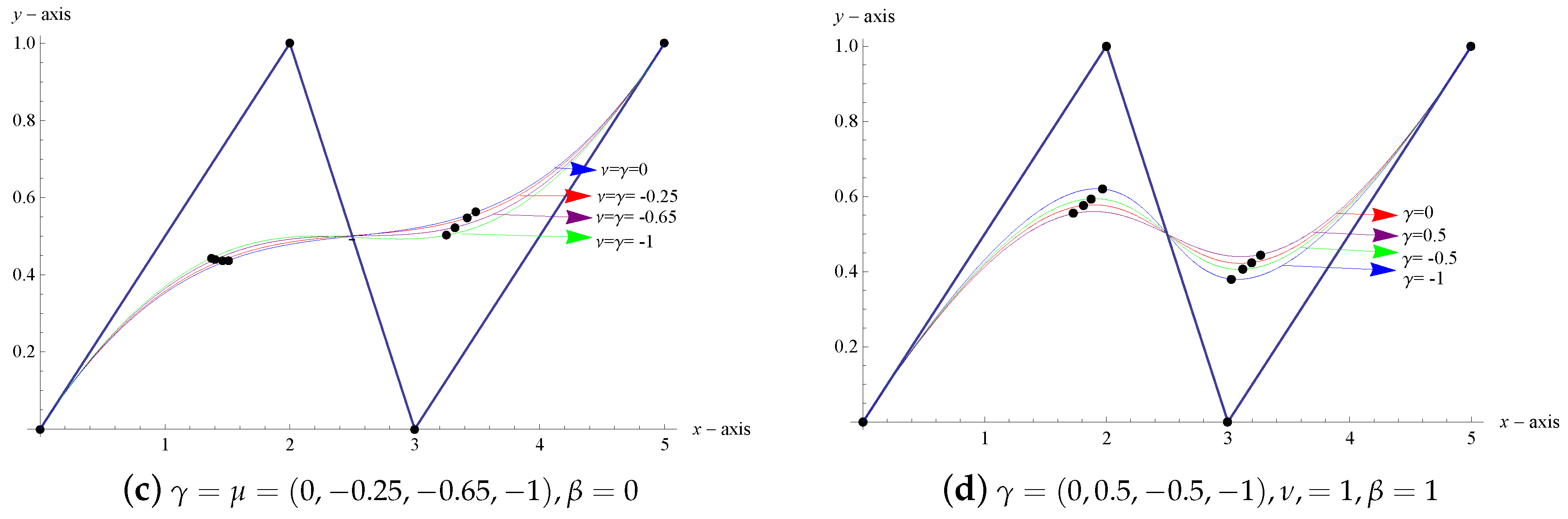
Since, the GHT-Bézier curve possesses three different shape parameters, by varying these three shape parameters, we can see the beautiful influence on the red, blue, green, and purple (thin) lines. The black dots on these curves show the linearity of the curves. Hence, Figure 2 depicts the influence of shape parameters on the GHT-Bézier curve.

Theorem 2.

GHT-Bézier curves possess the various properties like the convex hull property, symmetry, shape adjustable property, and variation diminishing property.

Proof. 

The proof of these properties is as described in [15].  □

3. The Geometric Significance of Shape Parameters

3.1. Correlation between a Fixed Point on the Curves and Shape Parameters

By using the definition of GHT-Bernstein basis functions and GHT-Bézier curves, we know that the cubic HT-Bézier curve $S(\theta ;\nu ,\beta ,\gamma )={\sum }_{i=0}^3{P}_i^{*}{q}_{i,n}\left(\theta \right)$ is a function having shape parameters. Therefore, we have:

$$\frac{\partial S\left(\theta \right)}{\partial \nu }=e^{\gamma \theta }(1-sin\left(\frac{\pi }{2}\theta \right))sin\left(\frac{\pi }{2}\theta \right)((-1+\theta )P_0^{*}+(1-2\theta )P_1^{*}+\theta P_2^{*})$$

$$\frac{\partial S\left(\theta \right)}{\partial \beta }=e^{\gamma (1-\theta )}(-1+cos\left(\frac{\pi }{2}\theta \right))cos\left(\frac{\pi }{2}\theta \right)((-1+\theta )P_1^{*}+(1-2\theta )P_2^{*}+\theta P_3^{*})$$

$$\frac{\partial S\left(\theta \right)}{\partial \gamma }=\left\{\begin{array}{c}{e}^{-\gamma \theta }(-e^{2\gamma \theta }\theta (1-sin\left(\frac{\pi }{2}\theta \right))(-1+\nu sin\left(\frac{\pi }{2}\theta \right))((-1+\theta )P_0^{*}+(1-2\theta )P_1^{*}+\theta P_2^{*})\hfill \\ +2e^{\gamma }(-1+\theta )(-1+\beta cos\left(\frac{\pi }{2}\theta \right))si{n}^2\left(\frac{\pi \theta }{4}\right)((-1+\theta )P_1^{*}+(1-2\theta )P_2^{*}+\theta P_3^{*})).\hfill \end{array}\right.$$

By concluding the above relationship, we can see that by changing the shape parameters, the fixed point on the curves change linearly for an unmovable control polygon. Figure 2 depicts the graph on which the black dots are given. These points corresponds to $S\left(0.3\right)$ on the left-hand side and $S\left(0.7\right)$ on right-hand side. We can see that by changing the shape parameters, the points on these curves change in a linear way.

3.2. Affiliation between GHT-Bézier Curves and Shape Parameters

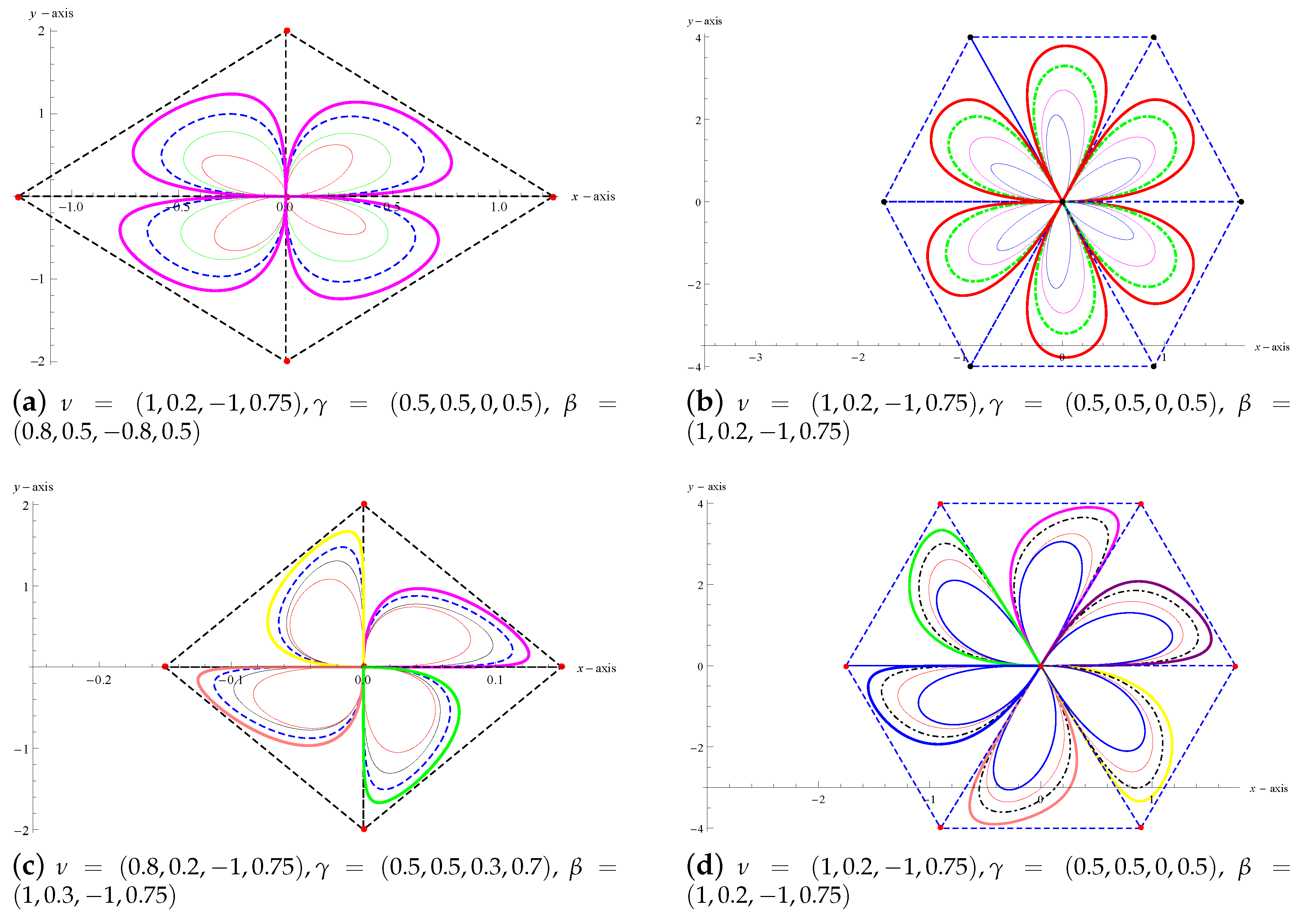
It was already described that the above-mentioned properties of GHT-Bézier curves illustrate that these remarkable curves can be attained according to our own desire by varying different shape parameters in their domain. Therefore, the alteration of these shape parameters can afford us an extraordinary beautification and attraction in the figures. Figure 3 shows the affiliation between the shape parameters and GHT-Bézier curves. By considering the minimum value of shape parameters, all the curves will be very close to the origin, but as we increase the values of these parameters, the curves will move away from the origin and near to the control polygon. Since GHT-Bézier curves have three distinct shape parameters, we can adjust and beautify the figures according to our own choice. Figure 3 represents the beautification of multiple colored GHT-Bézier curves of various degrees having distinct shape parameters and the influence of these shape parameters, and the shape control of the curves is also obvious in these figures. All these figures lie in the convex hull of the control polygon.

4. Continuity Constraints of GHT-Bézier Curves

In CAD/CAM systems, the construction of complex curves and figures is a very difficult process by using the $C^2$ and $G^2$ continuity conditions of traditional Bézier curves. While the GHT-Bézier curve has three different shape parameters, has great smoothness, and can be easily bent by adjusting the shape parameters according to our choice, it helps us to construct various complex curves by using parametric and geometric continuity constraints, which cannot be executed by classical Bézier curves.

Consider any two adjacent GHT-Bézier curves, which can be defined as:

$$\left\{\begin{array}{c}{S}_1(\theta ;{\nu }_1,{\beta }_1,{\gamma }_1)=\sum _{i=0}^n{P}_i^{*}{q}_{i,n}\left(\theta \right),0\le \theta \le 1,n\ge 3\hfill \\ S_2(\theta ;{\nu }_2,{\beta }_2,{\gamma }_2)=\sum _{j=0}^m{Q}_j^{*}{q}_{j,m}\left(\theta \right),0\le \theta \le 1,m\ge 3\hfill \end{array}\right.$$

(9)

where $P_i^{*}$, $(i=0,1,2,3,\dots ..,n)$ and $Q_j^{*}$, $(j=0,1,2,3,\dots .,m)$ are the control points of these two adjacent GHT-Bézier curves, $q_{i,n}\left(\theta \right)$ and $q_{j,m}\left(\theta \right)$ are GHT-Bernstein basis functions of degree n and m, respectively, and ${\nu }_1,{\beta }_1,{\gamma }_1$ and ${\nu }_2,{\beta }_2,{\gamma }_2$ are the shape parameters of curves.

4.1. Parametric Continuity Constraints of GHT-Bézier Curves

Theorem 3.

Given two GHT-Bézier curves $S_1\left(\theta \right)={\sum }_{i=0}^n{P}_i^{*}{q}_{i,n}\left(\theta \right)$ and $S_2\left(\theta \right)={\sum }_{j=0}^m{Q}_j^{*}{q}_{j,m}\left(\theta \right)$ of the same degree, the necessary and sufficient conditions for parametric continuity at the joints are given as follows:

1.

For $C^0$ continuity:

$$Q_0^{*}=P_n^{*}$$

(10)

2.

For $C^1$ continuity:

$$\left\{\begin{array}{c}{Q}_0^{*}=P_n^{*}\hfill \\ Q_1^{*}=P_n^{*}+\frac{(2n-4)+\pi (1+{\beta }_1)-2\gamma 1}{(2n-4)+\pi (1+{\nu }_2)-2\gamma 2}(P_n^{*}-P_{n-1}^{*})\hfill \end{array}\right.$$

(11)

3.

For the $C^2$ continuity condition, we have:

$$\left\{\begin{array}{c}{Q}_0^{*}=P_n^{*},\hfill \\ Q_1^{*}=P_n^{*}+\frac{(2n-4)+\pi (1+{\beta }_1)-2{\gamma }_1}{(2n-4)+\pi (1+{\nu }_2)-2{\gamma }_2}(P_n^{*}-P_{n-1}^{*}),\hfill \\ Q_2^{*}=[\{-4(n-2)(n-3)+8(n-2){\gamma }_1-4(n-2)({\beta }_1+1)\pi +e^{{\gamma }_1}{\pi }^2({\nu }_1-1)\}{P}_{n-2}^{*}\hfill \\ -\{4\pi (1+{\beta }_1)({\gamma }_1-4(n-2))-4({\gamma }_1({\gamma }_1-4(n-2))+2(n-2)(n-3))+{\pi }^2(-2{\beta }_1+e^{{\gamma }_1}\hfill \\ ({\nu }_1-1)\left)\right\}{P}_{n-1}^{*}+\{-4(n-2)\pi {\beta }_1-2{\pi }^2{\beta }_1+8(n-2){\gamma }_1+4\pi {\gamma }_1+4\pi {\beta }_1{\gamma }_1-4{\gamma }_1^2-8(n-2){\gamma }_2\hfill \\ -4\pi {\gamma }_2+4{\gamma }_2^2+4(n-2)\pi {\nu }_2+2{\pi }^2{\nu }_2-4\pi {\gamma }_2{\nu }_2\}{P}_n^{*}+\frac{1}{a}]b\hfill \\ where\hfill \\ a=(2(n-2)+\pi -2{\gamma }_2+\pi {\nu }_2)[-4(2(n-2)(n-3)+({\gamma }_2-4(n-2)){\gamma }_2)+{\pi }^2(e^{{\gamma }_2}({\beta }_2-1)\hfill \\ -2{\nu }_2)+4\pi ({\gamma }_2-2(n-2))(1+{\nu }_2)\left]\right(-(2(n-2)+\pi +\pi {\beta }_1-2{\gamma }_1)P_{n-1}^{*}+(-2(-2(n-2)+{\gamma }_1\hfill \\ +{\gamma }_2)+\pi (2+{\beta }_1+{\nu }_2)\left)P_n^{*}\right)\hfill \\ and\hfill \\ b=\frac{1}{(8(n-2){\gamma }_2-4(n-2)(n-3)-4(n-2)\pi (1+{\nu }_2)+{\pi }^2{e}^{{\gamma }_2}({\beta }_2-1))}\hfill \end{array}\right.$$

(12)

4.

For $C^3$ continuity conditions, we used $C^2$ continuity constraints and also obtained a new fourth control point $Q_3^{*}$ in $C^3$ continuity. Therefore, we have:

$$\left\{\begin{array}{c}{Q}_3^{*}=\frac{-e^{-{\gamma }_2}}{6{\pi }^2(1-{\beta }_2)}[-6e^{{\gamma }_1}{\pi }^2(-1+{\nu }_1)P_0^{*}+6(-2{\pi }^2{\beta }_1+4\pi (1+{\beta }_1){\gamma }_1-4{\gamma }_1^2+e^{{\gamma }_1}{\pi }^2(2+{\gamma }_1)(-1\hfill \\ +{\nu }_1\left)\right)P_1^{*}-({\pi }^3(1+{\beta }_1)+12{\pi }^2{\beta }_1(-2+{\gamma }_1)-12\pi (1+{\beta }_1)(-4+{\gamma }_1){\gamma }_1+8(-6+{\gamma }_1){\gamma }_1^2+6e^{{\gamma }_1}\hfill \\ {\pi }^2(1+{\gamma }_1)(-1+{\nu }_1))P_2^{*}+(2{\pi }^3-12{\pi }^2{\beta }_1+{\pi }^3{\beta }_1+24\pi {\gamma }_1+24\pi {\beta }_1{\gamma }_1+12{\pi }^2{\beta }_1{\gamma }_1-24{\gamma }_1^2\hfill \\ -12\pi {\gamma }_1^2-12\pi {\beta }_1{\gamma }_1^2+8{\gamma }_1^3+24\pi {\gamma }_2-24{\gamma }_2^2-12\pi {\gamma }_2^2+8{\gamma }_2^3-12{\pi }^2{\nu }_2+{\pi }^3{\nu }_2+24\pi {\gamma }_2{\nu }_2+\hfill \\ 12{\pi }^2{\gamma }_2{\nu }_2-12\pi {\gamma }_2^2{\nu }_2)P_3^{*}-\frac{1}{{\eta }_1}]\hfill \\ where\hfill \\ {\eta }_1=(2+\pi +-2{\gamma }_2+\pi {\nu }_2)[8{\gamma }_2^2(-6+{\gamma }_2)+6e^{{\gamma }_2}{\pi }^2(-1+{\beta }_2)(1+{\gamma }_2)+12{\pi }^2(-2+{\gamma }_2){\nu }_2+{\pi }^3\hfill \\ (1+{\nu }_2)-12\pi (-4+{\gamma }_2){\gamma }_2(1+{\nu }_2)\left]\right(-(2+\pi +\pi {\beta }_1-2{\gamma }_1)P_2^{*}+(-2(-2+{\gamma }_1+{\gamma }_2)+\pi \hfill \\ (2+{\beta }_1+{\nu }_2)\left)\right)P_3^{*}+\frac{a}{e^{{\gamma }_2}{\pi }^2(-1+{\beta }_2)+8{\gamma }_2-4\pi (1+{\nu }_2)},\hfill \\ a=6(-4{\gamma }_2^2+e^{{\gamma }_2}{\pi }^2(-1+{\beta }_2)(2+{\gamma }_2)-2{\pi }^2{\nu }_2+4\pi {\gamma }_2(1+{\nu }_2))\left\{\right(-4\pi (1+{\beta }_1)+8{\gamma }_1+e^{{\gamma }_1}{\pi }^2\hfill \\ (-1+{\nu }_1))P_1^{*}-(4\pi (1+{\beta }_1)(-2+{\gamma }_1)-4(-4+{\gamma }_1){\gamma }_1+{\pi }^2(-2{\beta }_1+e^{{\gamma }_1}(-1+{\nu }_1)))P_2^{*}+(-4\pi {\beta }_1\hfill \\ -2{\pi }^2{\beta }_1+8{\gamma }_1+4\pi {\gamma }_1+4\pi {\beta }_1{\gamma }_1-4{\gamma }_1^2-8{\gamma }_2-4\pi {\gamma }_2+4{\gamma }_2^2+4\pi {\nu }_2+2{\pi }^2{\nu }_2-4\pi {\gamma }_2{\nu }_2)P_3^{*}+\frac{1}{b}\},\hfill \\ b=(2+\pi -2{\gamma }_2+\pi {\nu }_2)(-4(-4+{\gamma }_2){\gamma }_2+{\pi }^2(e^{{\gamma }_2}(-1+{\beta }_2)-2{\nu }_2)+4\pi (-2+{\gamma }_2)(1+{\nu }_2))\{-(2\hfill \\ +\pi +\pi {\beta }_1-2{\gamma }_1)P_2^{*}+(-2(-2+{\gamma }_1+{\gamma }_2)+\pi (2+{\beta }_1+{\nu }_2))P_3^{*}\}.\hfill \end{array}\right.$$

(13)

Proof. 

For the $C^0$ continuity of GHT-Bézier curves, we keep both the first and second curves equal at the final and initial point of the domain respectively as $S_1\left(1\right)=S_2\left(0\right)$ to obtain the control point $Q_0^{*}$.

Similarly, for $C^1$, $C^2$, and $C^3$ continuity conditions, we consider the first, second, and third derivative of both curves equal like $S_1^{{}^{\prime }}\left(1\right)=S_2^{{}^{\prime }}\left(0\right)$, $S_1^{{}^{″}}\left(1\right)=S_2^{{}^{″}}\left(0\right)$ as in [15] and $S_1^{{}^{‴}}\left(1\right)=S_2^{{}^{‴}}\left(0\right)$ to obtain the control points $Q_1^{*}$, $Q_2^{*}$, and $Q_3^{*}$ given in Equations (12) and (13), respectively.  □

4.2. Algorithm for the Construction of Curves by Parametric Continuity Constraints

A brief algorithm about the construction of complex curves by using continuity constraints is given in this section. As we know that the smooth curves by using continuity conditions can be easily obtained and by adjusting the shape parameters, we can easily modify the curve according to our own choice as in [42].

The procedure for the construction of complex figures by parametric continuity between two GHT-Bézier curve segments is given as follows:

• For any curve of degree n, we consider an initial curve like $S_1(\theta ;{\nu }_1,{\beta }_1,{\gamma }_1)$ with its shape parameters and $n+1$ control points.
• For $C^0$ continuity by keeping $S_1(1;{\nu }_1,{\beta }_1,{\gamma }_1)$ and $S_2(0;{\nu }_2,{\beta }_2,{\gamma }_2)$ equal, we have $P_n^{*}=Q_0^{*}$, and the remaining control points are left to the designer’s choice.
• For $C^1$ continuity, tangent vectors of both the initial and final curve segment will be equal at the first and last point, respectively. Then, we obtain a new control point $Q_1^{*}$ of the second curve segment, and remaining control points will be left to the designer’s choice.
• Similarly, for $C^2$ continuity constraints, we also keep the second derivative of both curve segments equal along with $C^1$ continuity conditions and obtain the control point $Q_2^{*}$ of the final curve while remaining control points are left to the designer’s choice.
• Finally, for $C^3$ continuity conditions, we consider the third derivative of both curves equal along with $C^2$ continuity constraints to obtain the control point $Q_3^{*}$, and remaining control points will be taken as the designer’s choice.

Hence, by using the above algorithm, any graphical figure can be obtained by using continuity conditions. Some constructions of figures are given below, which were obtained by using the above brief discussion.

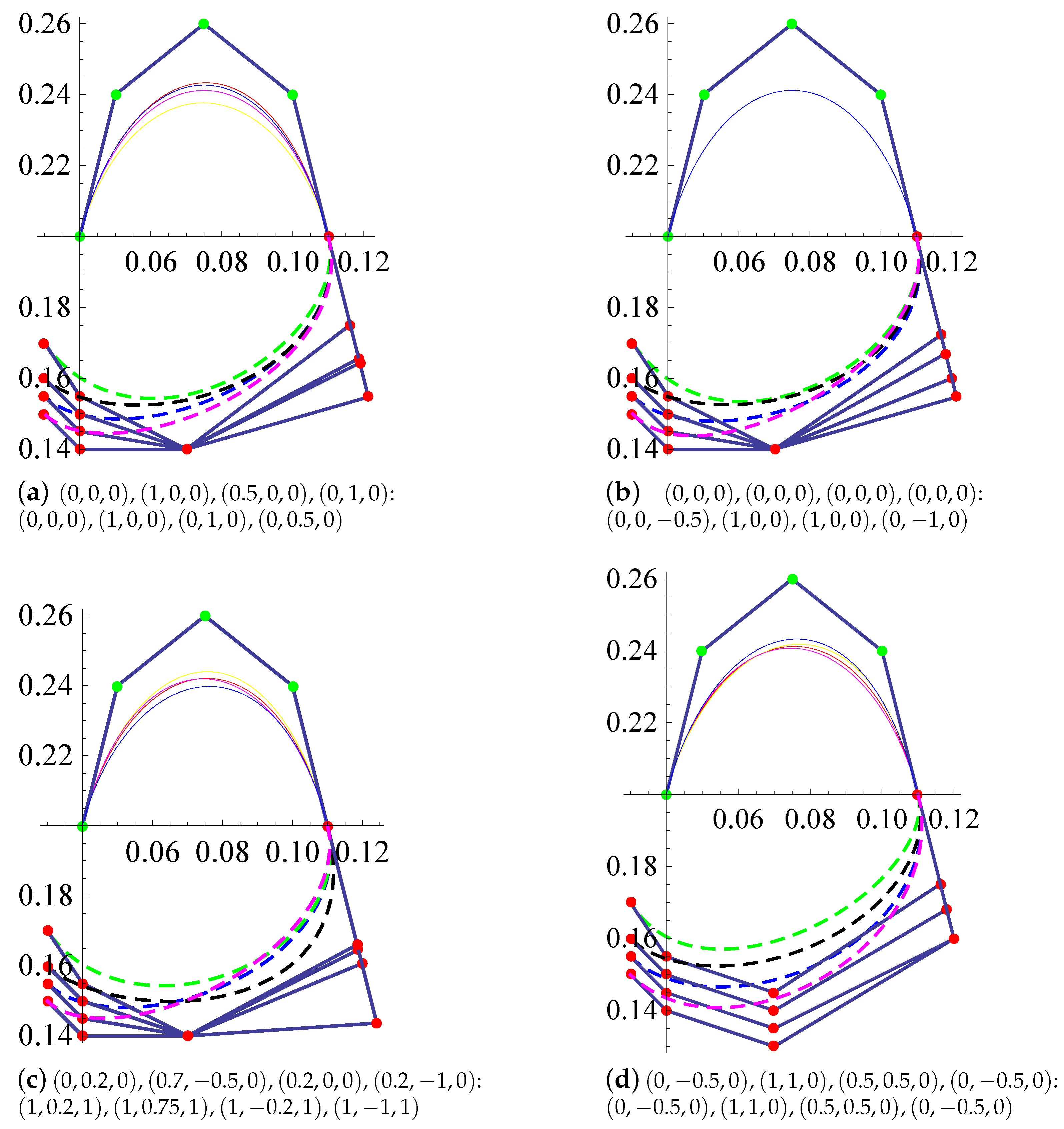
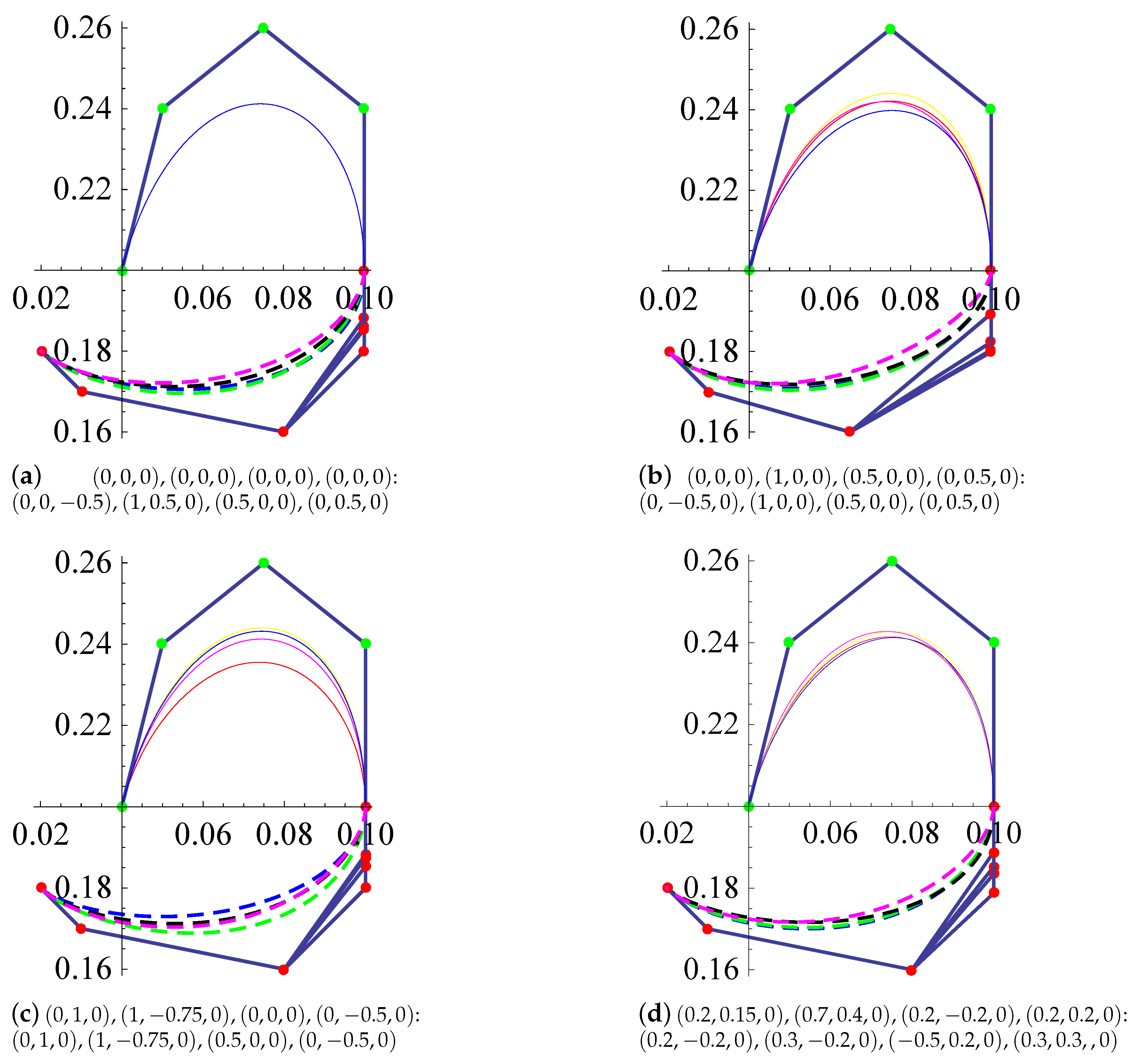
• $C^1$ continuity of GHT-Bézier curves:
  It is well known that the GHT-Bézier curve has three shape parameters, and we can construct various figures by using the continuity of any two curves. Therefore, consider any two quartic GHT-Bézier curves named as $W_1\left(\theta \right)$ and $W_2\left(\theta \right)$ containing shape parameters ${\nu }_1,{\beta }_1,{\gamma }_1$ and ${\nu }_2,{\beta }_2,{\gamma }_2$, respectively.

  $$\left\{\begin{array}{c}{W}_1(\theta ;{\nu }_1,{\beta }_1,{\gamma }_1)=\sum _{i=0}^4{P}_i^{*}{q}_{i,4}\left(\theta \right),0\le \theta \le 1\hfill \\ W_2(\theta ;{\nu }_2,{\beta }_2,{\gamma }_2)=\sum _{j=0}^4{Q}_j^{*}{q}_{j,4}\left(\theta \right),0\le \theta \le 1\hfill \end{array}\right.$$

  (14)

  Example 1.

  Figure 4 represents the GHT-Bézier curves that satisfy the parametric smooth continuity constraints at their joints.

  Here, in Figure 4, we consider the control points $P_0^{*}=(0.04,0.2)$, $P_1^{*}=(0.05,0.24)$, $P_2^{*}=(0.075,0.26)$, $P_3^{*}=(0.1,0.24)$, and $P_4^{*}=(0.11,0.2)$ to construct the thin curves, then the dotted curves will be obtained by $C^1$ continuity conditions; where $Q_0^{*}$ and $Q_1^{*}$ were obtained from continuity conditions and the last three control points could be adjusted according to our own choice. All these multiple thin and dotted curves could be attained by the variation of shape parameters. The different values of shape parameters are mentioned underneath the figures.
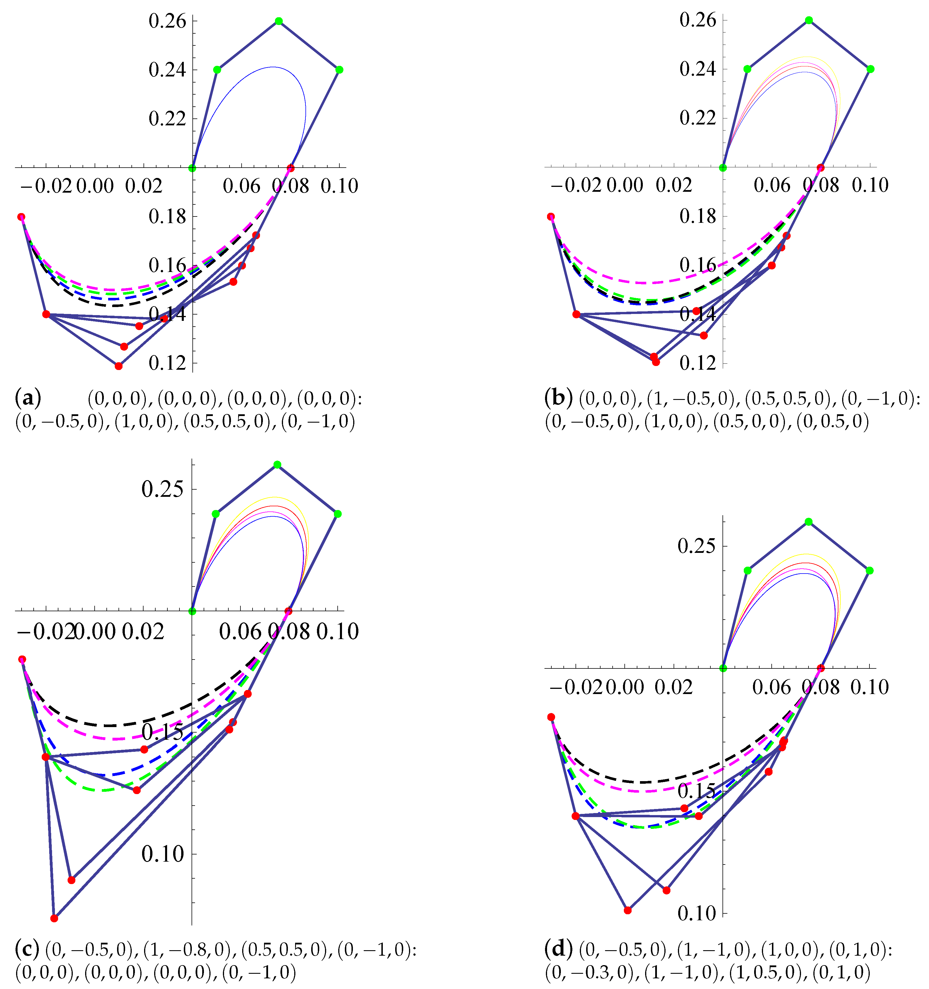
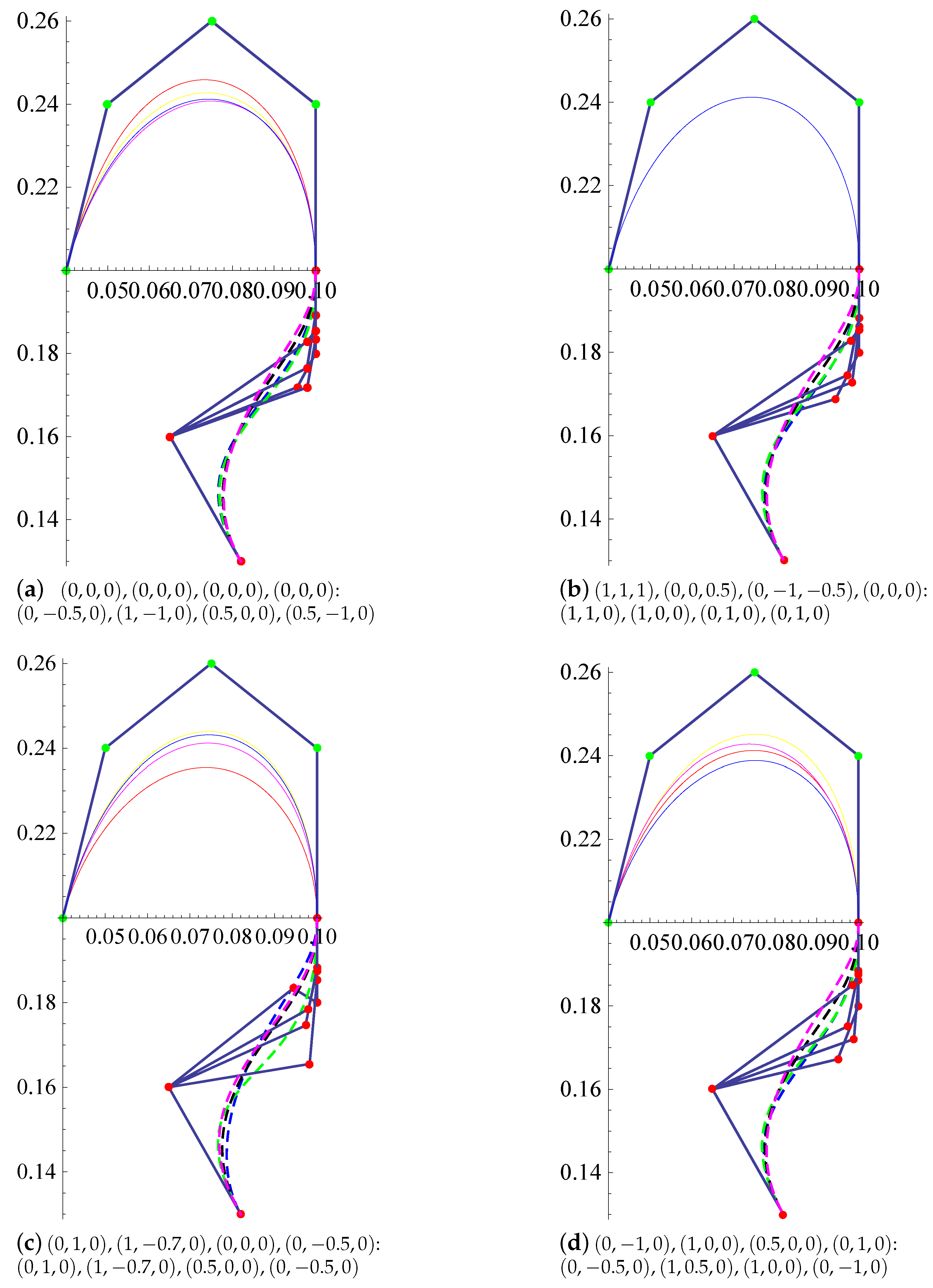
• $C^2$ continuity of GHT-Bézier curves:
  As we discussed above the $C^1$ continuity of the curves, now were turn to elaborate on the $C^2$ continuity of the curves. For this continuity, we again consider two quartic GHT-Bézier curves given in Equation (14) with three different shape parameters. We can also construct various complex curves by using $C^2$ continuity constraints. All the conditions are described above in Theorem 3.

  Example 2.

  In Figure 5, we chose these values of control points $P_0^{*}=(0.04,0.2)$, $P_1^{*}=(0.05,0.24)$, $P_2^{*}=(0.075,0.26)$, $P_3^{*}=(0.1,0.24)$, and $P_4^{*}=(0.08,0.2)$ to obtain the various curves. Now, by using $C^2$ continuity conditions, the graphical representation of curves is presented. The last two control points of the second curve have to be taken according to our own choice.

  All the thin lines were obtained by adjusting the control points of curve $W_1\left(\theta \right)$ while the dotted lines were obtained by using $C^2$ continuity conditions and the control points of the curve $W_2\left(\theta \right)$. Here, the last two control points of these curves could be adjusted according to our own choice. The shape parameters of each figure are given in the form of three tuples. The first four values under each figure are the values of $({\nu }_1,{\gamma }_1,{\beta }_1)$, while the next four values are of $({\nu }_2,{\gamma }_2,{\beta }_2)$.
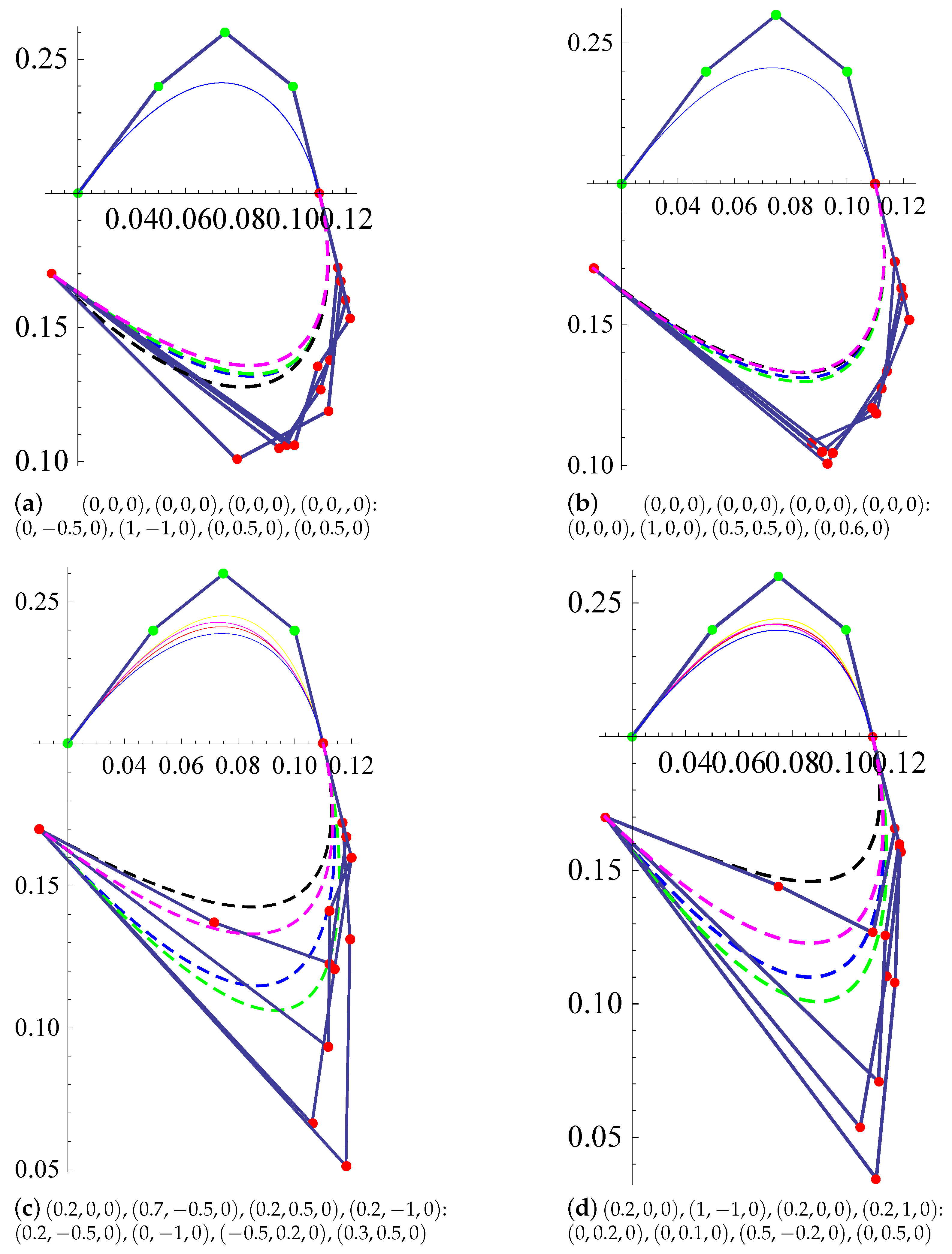
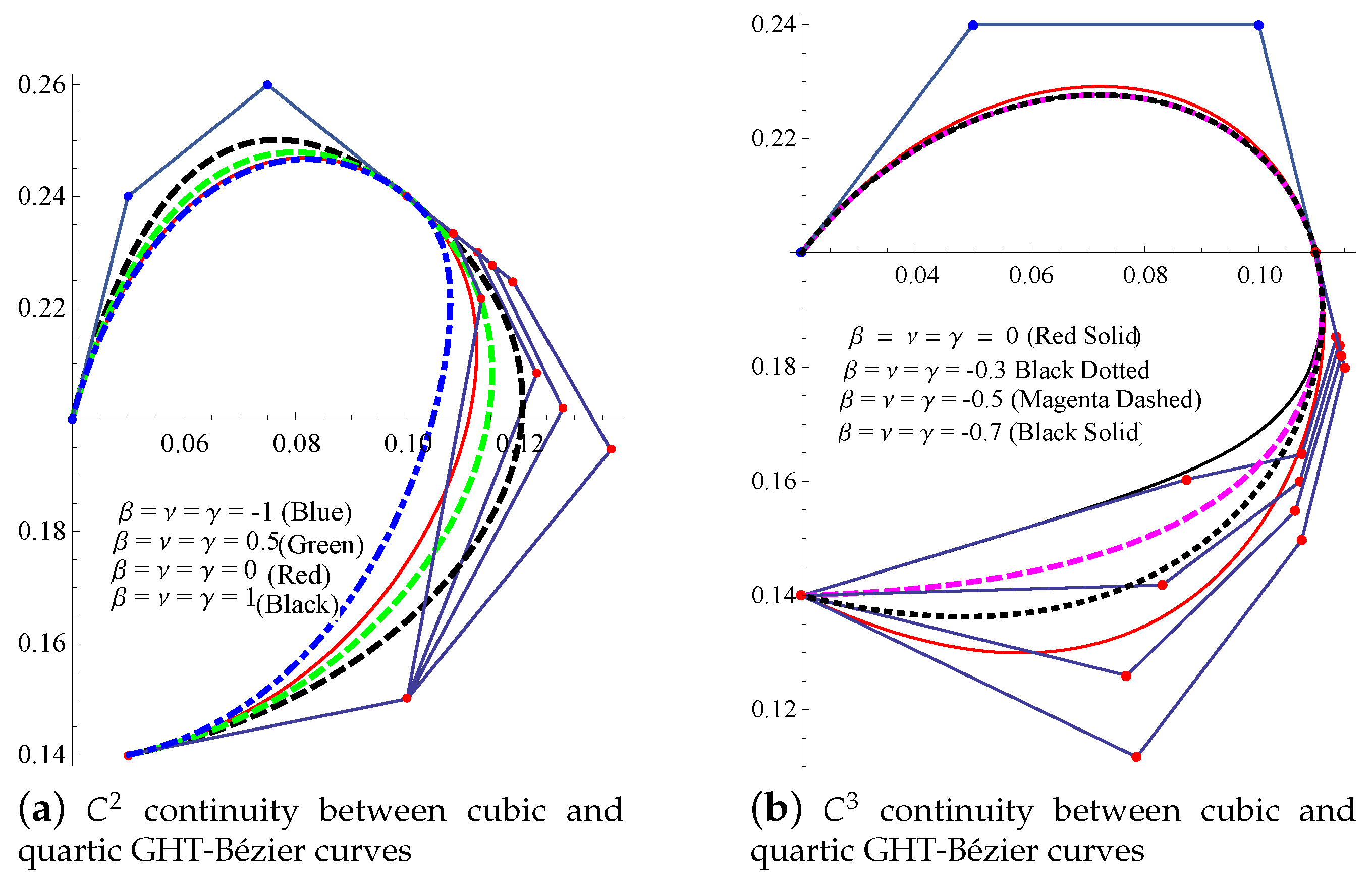
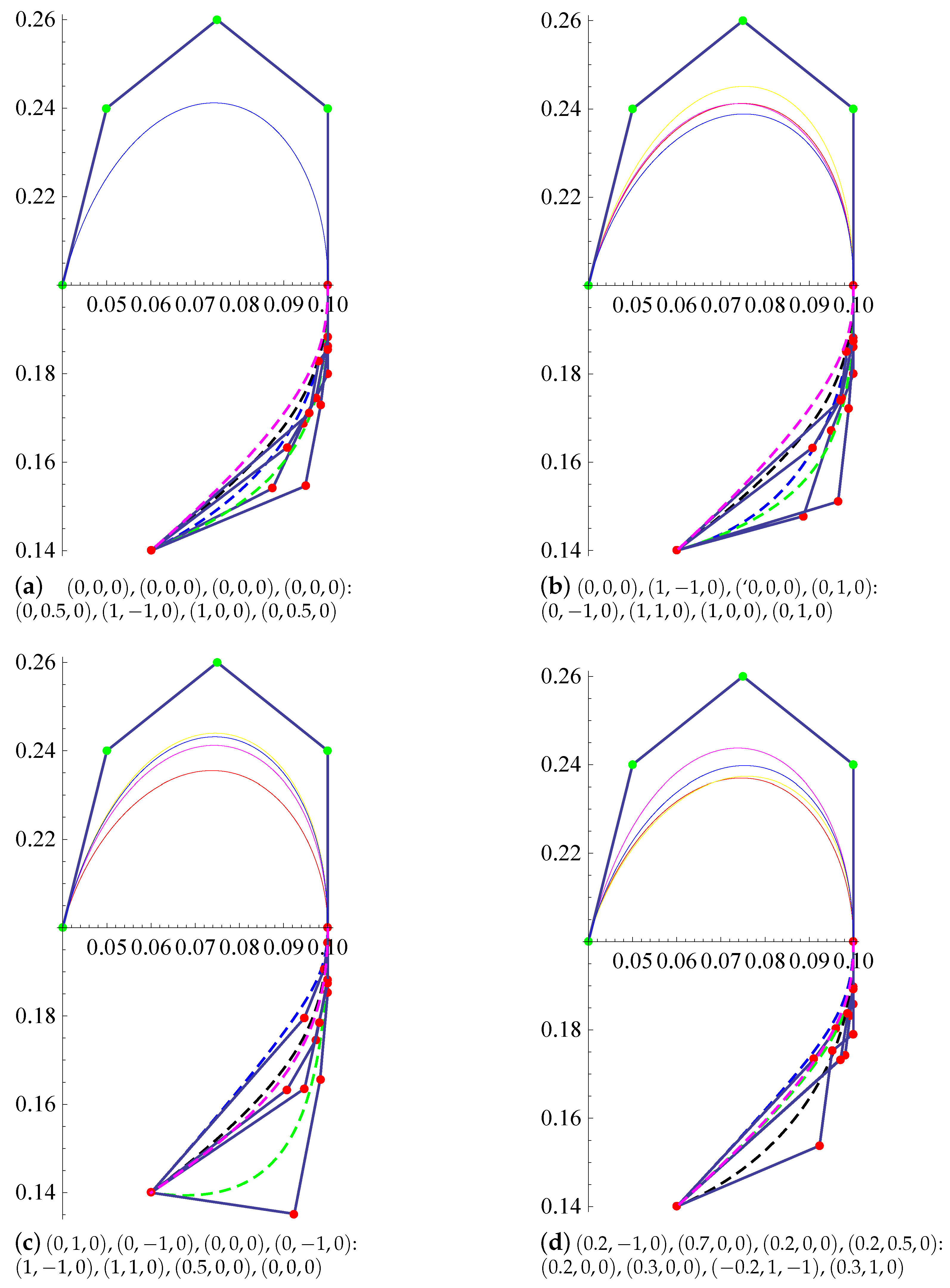
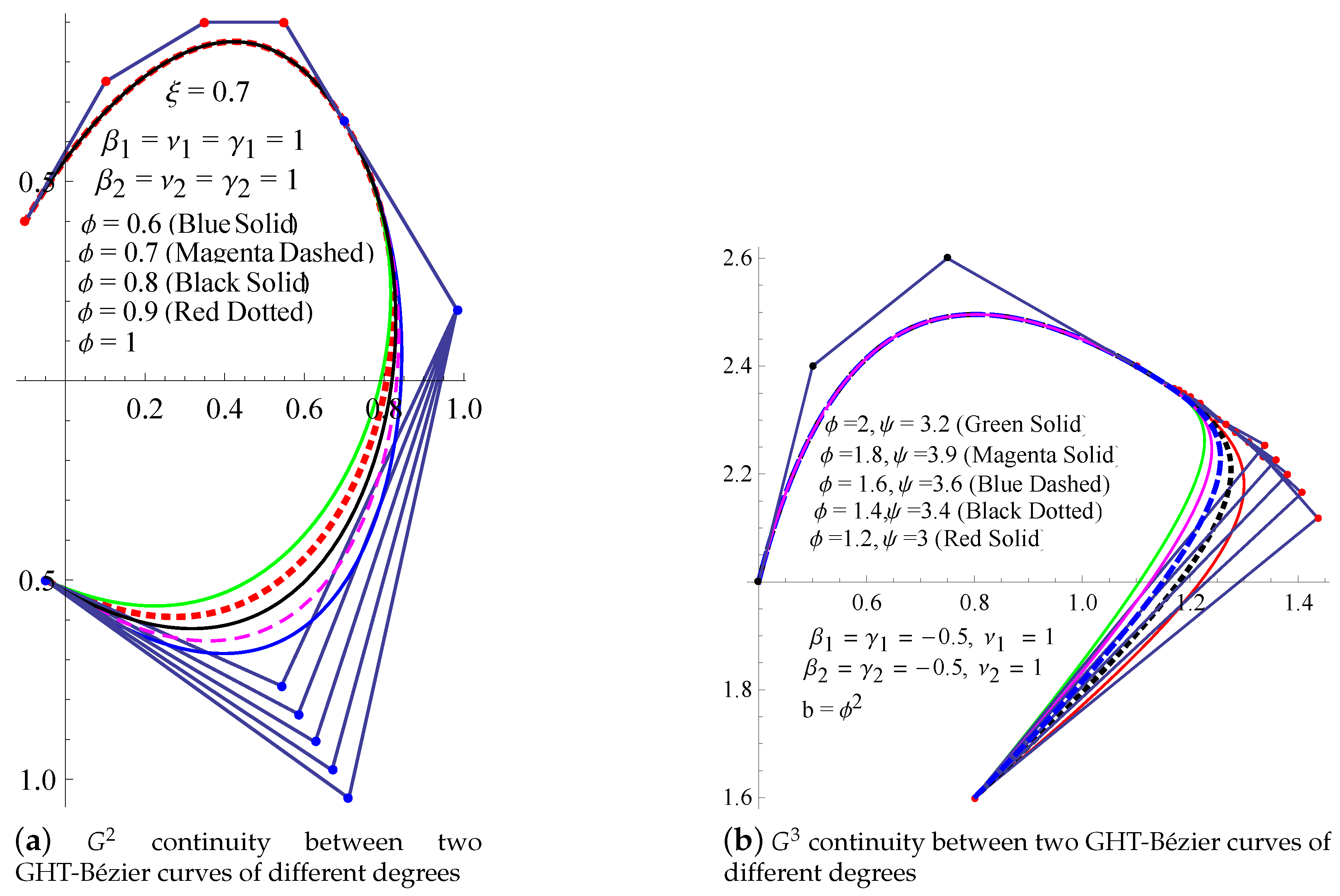
• $C^3$ continuity of GHT-Bézier curves:

  Example 3.

  Consider any two quartic GHT-Bézier curves named as $W_1\left(\theta \right)$ and $W_2\left(\theta \right)$ given in Equation (14) having three different shape parameters. All thin curves were obtained by using the definition of the first curve, and the second curve was obtained by using continuity conditions. We just needed to adjust the last control point of the second curve. Moreover, multi-valued shape parameters are given underneath the figures, which helped us to attain various curves at different positions. Figure 6 depicts the $C^3$ continuity of curves by varying different shape parameters, and the shape parameters are mentioned under each figure.

  Example 4.

  As discussed above, we can construct various GHT-Bézier curves of the same/different degrees by the procedure given in the above algorithms for the construction of curves by parametric continuity. Here, Figure 7 represents the $C^2$ and $C^3$ continuity between a cubic and quartic GHT-Bézier curve (curves of different degrees) with shape parameters ${\beta }_1={\beta }_2=\beta$, ${\gamma }_1={\gamma }_2=\gamma$ and ${\nu }_1={\nu }_2=\nu$. For $C^2$ continuity, the control points for the initial cubic GHT-Bézier curve are $P_0^{*}=(0.04,0.2)$, $P_1^{*}=(0.05,0.24)$, $P_2^{*}=(0.075,0.26)$, and $P_3^{*}=(0.1,0.24)$, while the first three control points for the second quartic GHT-Bézier curve can be obtained by $C^2$ continuity condition, and the remaining two control points can be taken according to our own choice such as $Q_3^{*}=(0.1,0.15)$ and $Q_4^{*}=(0.05,0.14).$ Similarly, for $C^3$ continuity conditions, the control points for the initial cubic GHT-Bézier curve are $P_0^{*}=(0.02,0.2)$, $P_1^{*}=(0.05,0.24)$, $P_2^{*}=(0.1,0.24)$, and $P_3^{*}=(0.11,0.2)$, while the second GHT-Bézier curve was obtained by applying the $C^3$ continuity condition only on the last control point taken as $Q_4^{*}=(0.02,0.14).$ Variation in the curves could be obtained by varying the values of shape parameters as mentioned with the figures.

4.3. Geometric Continuity Constraints of GHT-Bézier Curves

Just like parametric continuity, geometric continuity also helps us to construct different complex figures. It is superior to parametric continuity because it gives us more smoothness due to the scale factor.

Theorem 4.

Consider any two GHT-Bézier curves $S_1(\theta ;{\nu }_1,{\beta }_1,{\gamma }_1)$ and $S_2(\theta ;{\nu }_2,{\beta }_2,{\gamma }_2)$ of the same degree with their shape parameters and control points $P_i^{*}$ and $Q_j^{*}$, respectively. These curves meet to the geometric continuity constraints if and only if:

$$\left\{\begin{array}{c}{Q}_0^{*}=P_n^{*}\hfill \\ Q_1^{*}=P_n^{*}+\frac{((2n-4)+\pi (1+{\beta }_1)-2{\gamma }_1)}{((2n-4)+\pi (1+{\nu }_2)-2{\gamma }_2)\varphi }(P_n^{*}-P_{n-1}^{*})\hfill \\ Q_2^{*}=[\{-4(n-2)(n-3)+8(n-2){\gamma }_1-4(n-2)({\beta }_1+1)\pi +e^{{\gamma }_1}{\pi }^2({\nu }_1-1)\}{P}_{n-2}^{*}\hfill \\ -\{4\pi (1+{\beta }_1)({\gamma }_1-2(n-2))-4({\gamma }_1({\gamma }_1-4(n-2))+2(n-2)(n-3))+{\pi }^2(-2{\beta }_1+e^{{\gamma }_1}({\nu }_1-1))\}{P}_{n-1}^{*}\hfill \\ -2\{2(n-2)+\pi +\pi {\beta }_1-2{\gamma }_1\}(P_{n-1}^{*}-P_n^{*})-4(n-2)(n-3)P_n^{*}-4(n-2)\pi P_n^{*}\hfill \\ -4(n-2)\pi {\beta }_1{P}_n^{*}-2\pi (\pi {\beta }_1-4(n-2){\gamma }_1)P_n^{*}+(4\pi {\beta }_1{\gamma }_1-4{\gamma }_1^2+4\pi {\gamma }_1)P_n^{*}+4(n-2)(n-3)\xi P_n^{*}\hfill \\ +4(n-2)\pi \xi P_n^{*}-8(n-2){\gamma }_2\xi P_n^{*}+(-4\pi {\gamma }_2\xi +4{\gamma }_2^2\xi +4(n-2)\pi \xi {\nu }_2+2{\pi }^2\xi {\nu }_2-4\pi \xi {\gamma }_2{\nu }_2)P_n^{*}+\frac{1}{J}]\epsilon \hfill \\ where\hfill \\ J=(2(n-2)+\pi -2{\gamma }_2+\pi {\nu }_2)\varphi [-4(2(n-2)(n-3)+({\gamma }_2-4(n-2)){\gamma }_2)+{\pi }^2(e^{{\gamma }_2}({\beta }_2-1)-2{\nu }_2)\hfill \\ +4\pi ({\gamma }_2-2(n-2))(1+{\nu }_2)\left]\xi \right(-(2(n-2)+\pi +\pi {\beta }_1-2{\gamma }_1)P_{n-1}^{*}+(2(n-2)+\pi +\pi {\beta }_1-2{\gamma }_1\hfill \\ +(2(n-2)+\pi -2{\gamma }_2+\pi {\nu }_2)\varphi \left)P_n^{*}\right)\hfill \\ and\hfill \\ \epsilon =\frac{1}{(8(n-2){\gamma }_2-4(n-2)(n-3)-4(n-2)\pi (1+{\nu }_2)+{\pi }^2{e}^{{\gamma }_2}({\beta }_2-1))\xi }\hfill \end{array}\right.$$

(15)

where ϕ is any positive real number and ε and J are the terms that are used to generalize the control point $Q_2^{*}$ in $G^2$ continuity.

Similarly, for $G^3$ continuity conditions and for both curves having degree three, we have:

$$\left\{\begin{array}{c}{Q}_3^{*}=\frac{-e^{-{\gamma }_2}}{6{\pi }^2\psi (1-{\beta }_2)}[-6e^{{\gamma }_1}{\pi }^2(-1+{\nu }_1)P_0^{*}+6(-2{\pi }^2{\beta }_1+4\pi (1+{\beta }_1){\gamma }_1-4{\gamma }_1^2+e^{{\gamma }_1}{\pi }^2(2+{\gamma }_1)(-1+{\nu }_1))\hfill \\ P_1^{*}-({\pi }^3(1+{\beta }_1)+12{\pi }^2{\beta }_1(-2+{\gamma }_1)-12\pi (1+{\beta }_1)(-4+{\gamma }_1){\gamma }_1+8(-6+{\gamma }_1){\gamma }_1^2+6e^{{\gamma }_1}{\pi }^2(1+{\gamma }_1)\hfill \\ (-1+{\nu }_1))P_2^{*}-4(2+\pi (1+{\beta }_1)-2{\gamma }_1)(P_2^{*}-P_3^{*})+{\pi }^3{P}_3^{*}+(-12{\pi }^2{\beta }_1+{\pi }^3{\beta }_1+24\pi {\gamma }_1+24\pi {\beta }_1{\gamma }_1-\hfill \\ 24{\gamma }_1^2+12{\pi }^2{\beta }_1{\gamma }_1-12\pi {\gamma }_1^2-12\pi {\beta }_1{\gamma }_1^2+8{\gamma }_1^3+{\pi }^3\psi +24\pi {\gamma }_2\psi -24\psi {\gamma }_2^2-12\pi \psi {\gamma }_2^2+8{\gamma }_2^2\psi -12{\pi }^2{\nu }_2\psi \hfill \\ +{\pi }^3{\nu }_2\psi +24\pi {\gamma }_2{\nu }_2\psi +12{\pi }^2{\gamma }_2{\nu }_2\psi -12\pi {\gamma }_2^2{\nu }_2)P_3^{*}-\frac{1}{{\eta }_1}-\frac{1}{{\eta }_2}]\hfill \end{array}\right.$$

(16)

$$\left\{\begin{array}{c}where,\hfill \\ {\eta }_1=6\xi {\varphi }^2((-4\pi (1+{\beta }_1)+8{\gamma }_1+e^{{\gamma }_1}{\pi }^2(-1+{\nu }_1))P_1^{*}+(-2\pi (1+{\beta }_1)(-3+2{\gamma }_1)+4(-1-3{\gamma }_1+{\gamma }_1^2)\hfill \\ +{\pi }^2(e^{{\gamma }_1}(1-{\nu }_1)+2{\beta }_1))P_2^{*}-2({\pi }^2{\beta }_1-\pi (1+{\beta }_1)(-1+2{\gamma }_1)+2(-1-{\gamma }_1+{\gamma }_1^2))P_3^{*}),\hfill \\ {\eta }_2=(2+\pi +-2{\gamma }_2+\pi {\nu }_2)\varphi (8{\gamma }_2^2(-6+{\gamma }_2)+6e^{{\gamma }_2}{\pi }^2(-1+{\beta }_2)(1+{\gamma }_2)+12{\pi }^2(-2+{\gamma }_2){\nu }_2+{\pi }^3(1+{\nu }_2)\hfill \\ -12\pi (-4+{\gamma }_2){\gamma }_2(1+{\nu }_2)\left)\psi \right(-(2+\pi +\pi {\beta }_1-2{\gamma }_1)P_2^{*}+(-2(-1+{\gamma }_1+(-1+{\gamma }_2)\varphi )+\pi (1+{\beta }_1+\varphi \hfill \\ (1+{\nu }_2)\left)\right)P_3^{*})+\frac{a}{\xi (e^{{\gamma }_2}{\pi }^2(-1+{\beta }_2)+8{\gamma }_2-4\pi (1+{\nu }_2))},\hfill \\ a=6(-4{\gamma }_2^2+e^{{\gamma }_2}{\pi }^2(-1+{\beta }_2)(2+{\gamma }_2)-2{\pi }^2{\nu }_2+4\pi {\gamma }_2(1+{\nu }_2))\psi \left\{\right(-4\pi (1+{\beta }_1)+8{\gamma }_1+e^{{\gamma }_1}{\pi }^2(-1+\hfill \\ {\nu }_1\left)\right)P_1^{*}-(4\pi (1+{\beta }_1)(-2+{\gamma }_1)-4(-4+{\gamma }_1){\gamma }_1+{\pi }^2(-2{\beta }_1+e^{{\gamma }_1}(-1+{\nu }_1)))P_2^{*}-2(2+\pi +\pi {\beta }_1-2{\gamma }_1)\hfill \\ (P_2^{*}-P_3^{*})+(-4\pi -4\pi {\beta }_1-2{\pi }^2{\beta }_1+8{\gamma }_1+4\pi {\gamma }_1+4\pi {\beta }_1{\gamma }_1-4{\gamma }_1^2+4\pi \xi -8{\gamma }_2\xi -4\pi {\gamma }_2\xi +4{\gamma }_2^2\xi +\hfill \\ 4\pi {\nu }_2\xi +2{\pi }^2{\nu }_2\xi -4\pi {\gamma }_2{\nu }_2\xi )P_3^{*}+\frac{1}{b}\},\hfill \\ b=(2+\pi -2{\gamma }_2+\pi {\nu }_2)\varphi (-4(-4+{\gamma }_2){\gamma }_2+{\pi }^2(e^{{\gamma }_2}(-1+{\beta }_2)-2{\nu }_2)+4\pi (-2+{\gamma }_2)(1+{\nu }_2))\xi \{-(2+\pi \hfill \\ +\pi {\beta }_1-2{\gamma }_1)P_2^{*}+(-2(-1+{\gamma }_1+(-1+{\gamma }_2)\varphi )+\pi (1+{\beta }_1+\varphi +{\nu }_2\varphi ))P_3^{*}\}.\hfill \end{array}\right.$$

(17)

where ${\eta }_1$, ${\eta }_2$, a, and b are the terms used to define the large value of control point $Q_3^{*}$ in $G^3$ continuity.

Proof. 

For the $G^0$ continuity condition, we keep both curves equal, i.e.,

$$S_1(1;{\nu }_1,{\beta }_1,{\gamma }_1)=S_2(0;{\nu }_2,{\beta }_2,{\gamma }_2)$$

and obtained the first control point of the second curve, i.e.,

$$Q_0^{*}=P_n^{*}.$$

For $G^1$ continuity constraints, we keep both curves equal and also the first derivative of both curves involving a scale factor such as,

$$\left\{\begin{array}{c}{S}_1(1;{\nu }_1,{\beta }_1,{\gamma }_1)=S_2(0;{\nu }_2,{\beta }_2,{\gamma }_2)\hfill \\ S_1^{{}^{\prime }}(1;{\nu }_1,{\beta }_1,{\gamma }_1)=\varphi S_2^{{}^{\prime }}(0;{\nu }_2,{\beta }_2,{\gamma }_2),\varphi >0.\hfill \end{array}\right.$$

By solving the above equation, we get:

$$Q_1^{*}=P_n^{*}+\frac{((2n-4)+\pi (1+{\beta }_1)-2{\gamma }_1)}{((2n-4)+\pi (1+{\nu }_2)-2{\gamma }_2)\varphi }(P_n^{*}-P_{n-1}^{*})$$

Now, for $G^2$ continuity, first we should fulfil the $G^1$ continuity conditions. One more necessary condition for the $G^2$ continuity condition is that the curvature of first curve at the last point and the second curve at the first point should be equal, i.e., ${\kappa }_1\left(1\right)={\kappa }_2\left(0\right)$.

Suppose that the curvature of $S_1(\theta ;{\nu }_1,{\beta }_1,{\gamma }_1)$ at the final point is ${\kappa }_1\left(1\right)$ and the curvature of $S_2(\theta ;{\nu }_2,{\beta }_2,{\gamma }_2)$ at the initial point is ${\kappa }_2\left(0\right)$, which is described as:

$$\left\{\begin{array}{c}{\kappa }_1\left(1\right)=\frac{S_1^{{}^{\prime }}(1;{\nu }_1,{\beta }_1,{\gamma }_1)\times S_1^{{}^{″}}(1;{\nu }_1,{\beta }_1,{\gamma }_1)}{|S_1^{{}^{\prime }}(1;{\nu }_1,{\beta }_1,{\gamma }_1){|}^3}\hfill \\ {\kappa }_2\left(0\right)=\frac{S_2^{{}^{\prime }}(0;{\nu }_1,{\beta }_1,{\gamma }_1)\times S_2^{{}^{″}}(0;{\nu }_1,{\beta }_1,{\gamma }_1)}{|S_2^{{}^{\prime }}(0;{\nu }_1,{\beta }_1,{\gamma }_1){|}^3}\hfill \end{array}\right.$$

Therefore, the reverse normal vector $L_1=S_1^{{}^{\prime }}\left(1\right)\times S_1^{{}^{″}}\left(1\right)$ of $S_1\left(\theta \right)$ and, vice versa, the normal vector $L_2=S_2^{{}^{\prime }}\left(0\right)\times S_2^{{}^{″}}\left(0\right)$ of $S_2\left(\theta \right)$ have the same direction. Therefore, these four vectors $S_1^{{}^{\prime }}\left(1\right)$, $S_2^{{}^{\prime }}\left(0\right)$, $S_2^{{}^{″}}\left(0\right)$ and $S_1^{{}^{″}}\left(1\right)$ are in same plane (coplanar) such that we have $S_1^{{}^{″}}\left(1\right)=\xi S_2^{{}^{″}}\left(0\right)+\varphi S_2^{{}^{\prime }}\left(0\right)$, where $\xi$ is any positive real number and $\xi ={\varphi }^2$. As:

$${\kappa }_1\left(1\right)=\frac{S_1^{{}^{\prime }}\left(1\right)\times S_1^{{}^{″}}\left(1\right)}{\left|\right|S_1^{{}^{\prime }}\left(1\right){\left|\right|}^3}=\frac{\xi \varphi (S_2^{{}^{\prime }}\left(0\right)\times S_2^{{}^{″}}\left(0\right))}{{\varphi }^3\left|\right|S_2^{{}^{\prime }}\left(0\right){\left|\right|}^3}=\frac{S_2^{{}^{\prime }}\left(0\right)\times S_2^{{}^{″}}\left(0\right)}{\left|\right|S_2^{{}^{\prime }}\left(0\right){\left|\right|}^3}={\kappa }_2\left(0\right)$$

we meet the $G^2$ continuity condition as described in [42].

After the derivation of the $G^2$ continuity condition, now we move to find the $G^3$ continuity condition at which the derivative of the curvature of the first curve at the final point and the second curve at the initial point will be the same, i.e., ${\kappa }_1^{{}^{\prime }}\left(1\right)=\varphi {\kappa }_2^{{}^{\prime }}\left(0\right)$. The first derivative of the curvature is:

$${\kappa }_1^{{}^{\prime }}\left(1\right)=\frac{\left|\right|S_1^{{}^{\prime }}\left(1\right){\left|\right|}^2\{S_1^{{}^{\prime }}\left(1\right)\times S_1^{{}^{‴}}\left(1\right)\}-3\{S_1^{{}^{\prime }}\left(1\right)\times S_1^{{}^{″}}\left(1\right)\}\{S_1^{{}^{\prime }}\left(1\right).S_1^{{}^{″}}\left(1\right)\}}{\left|\right|S_1^{{}^{\prime }}\left(1\right){\left|\right|}^5}$$

(18)

and:

$${\kappa }_2^{{}^{\prime }}\left(0\right)=\frac{\left|\right|S_2^{{}^{\prime }}\left(0\right){\left|\right|}^2\{S_2^{{}^{\prime }}\left(0\right)\times S_2^{{}^{‴}}\left(0\right)\}-3\{S_2^{{}^{\prime }}\left(0\right)\times S_2^{{}^{″}}\left(0\right)\}\{S_2^{{}^{\prime }}\left(0\right).S_2^{{}^{″}}\left(0\right)\}}{\left|\right|S_2^{{}^{\prime }}\left(0\right){\left|\right|}^5}.$$

(19)

We consider the conditions given as follows:

$$\left\{\begin{array}{c}{S}_1^{{}^{\prime }}\left(1\right)=\varphi S_2^{{}^{\prime }}\left(0\right),\hfill \\ S_1^{{}^{″}}\left(1\right)=\xi S_2^{{}^{″}}\left(0\right)+\varphi S_2^{{}^{\prime }}\left(0\right),\hfill \\ S_1^{{}^{‴}}\left(1\right)=\psi S_2^{{}^{‴}}\left(0\right)+3{\varphi }^2{S}_2^{{}^{″}}\left(0\right)+\varphi S^{{}^{\prime }}\left(0\right)\hfill \end{array}\right.$$

(20)

where $\psi ={\varphi }^3$ and $\xi ={\varphi }^2$ meet the $G^3$ continuity constraints. Consider,

$${\kappa }_1^{{}^{\prime }}\left(1\right)=\frac{\vartheta }{\left|\right|{\varphi }^5{S}_1^{{}^{\prime }}\left(0\right){\left|\right|}^5}$$

(21)

where:

$$\begin{array}{c}\vartheta =\left|\right|\varphi S_2^{{}^{\prime }}\left(0\right){\left|\right|}^2\{\varphi S_2^{{}^{\prime }}\left(0\right)\times (\psi S_2^{{}^{‴}}\left(0\right)+3{\varphi }^2{S}_2^{{}^{″}}\left(0\right)+\varphi S_2^{{}^{\prime }}\left(0\right))\}\hfill \\ \hspace{1em}\hspace{1em}\hspace{1em}\hspace{1em}\hspace{1em}\hspace{1em}\hspace{1em}\hspace{1em}\hspace{1em}\hspace{1em}\hspace{1em}\hspace{1em}\hspace{1em}\hspace{1em}-3\{\varphi S_2^{{}^{\prime }}\left(0\right)\times (\xi S_2^{{}^{″}}\left(0\right)+\varphi S_2^{{}^{\prime }}\left(0\right))\}\{\varphi S_2^{{}^{\prime }}\left(0\right).(\xi S_2^{{}^{″}}\left(0\right)+\varphi S_2^{{}^{\prime }}\left(0\right))\}\hfill \end{array}$$

Since $\left|\right|\phi z\left(\theta \right)\left|\right|=\left|\phi \right|\left|\right|z\left(\theta \right)\left|\right|$, we will obtain:

$$\vartheta =\psi {\varphi }^3\left|\right|S_2^{{}^{\prime }}\left(0\right){\left|\right|}^2\left(S_2^{{}^{\prime }}\left(0\right)\times S_2^{{}^{‴}}\left(0\right)\right)-3{\varphi }^6\left(S_2^{{}^{\prime }}\left(0\right)\times S_2^{{}^{″}}\left(0\right)\right)\left(S_2^{{}^{\prime }}\left(0\right).S_2^{{}^{″}}\left(0\right)\right)$$

and by substituting this value of $\vartheta$ in (21), we have:

$${\kappa }_1^{{}^{\prime }}\left(1\right)=\varphi \left\{\frac{\left|\right|S_2^{{}^{\prime }}\left(0\right){\left|\right|}^2\{S_2^{{}^{\prime }}\left(0\right)\times S_2^{{}^{‴}}\left(0\right)\}-3\{S_2^{{}^{\prime }}\left(0\right)\times S_2^{{}^{″}}\left(0\right)\}\{S_2^{{}^{\prime }}\left(0\right).S_2^{{}^{″}}\left(0\right)\}}{\left|\right|S_2^{{}^{\prime }}\left(0\right){\left|\right|}^5}\right\}=\varphi {\kappa }_2^{{}^{\prime }}\left(0\right).$$

(22)

 □

4.4. Algorithm for the Construction of Curves by Geometric Continuity Constraints

Like parametric continuity, a brief algorithm about the construction of complex curves by using geometric continuity conditions is given in this section. The procedure for the construction of figures by geometric smooth continuity between two GHT-Bézier curves is given as follows:

• For any curve of degree n, we consider an initial curve like $S_1(\theta ;{\nu }_1,{\beta }_1,{\gamma }_1)$ with its shape parameters and $n+1$ control points.
• Like $C^0$ continuity, by keeping $S_1(1;{\nu }_1,{\beta }_1,{\gamma }_1)$ and $S_2(0;{\nu }_2,{\beta }_2,{\gamma }_2)$ equal, we obtain the control point $Q_0^{*}$ for $G^0$ continuity, i.e., $P_n^{*}=Q_0^{*}$, and remaining control points of the second curve will be left to the designer’s choice.
• For $G^1$ continuity, both the initial and final curve segments with their tangent vectors will be equal at the last and first point of the domain, respectively, and an extra positive scale factor will be added with the tangent vector of the second curve as $S_1^{{}^{\prime }}\left(1\right)=\varphi S_2^{{}^{\prime }}\left(0\right)$ to obtain $Q_1^{*}$ in the $G^1$ continuity. The remaining control points will be left to the designer’s choice. The new curve will be obtained smoothly by using this condition.
• Similarly, for $G^2$ continuity conditions, a new point $Q_2^{*}$ will be obtained by using $S_1^{{}^{″}}\left(1\right)={\varphi }^2{S}_2^{{}^{″}}\left(0\right)+\varphi S_2^{{}^{\prime }}\left(0\right)$ as in [42] along with $G^1$ continuity conditions while remaining control points should be taken according to our own choice to construct any complex curve.
• Finally, for the construction of any curve by using $G^3$ continuity conditions, consider $S_1^{{}^{‴}}\left(1\right)=\psi S_2^{{}^{‴}}\left(0\right)+3{\varphi }^2{S}_2^{{}^{″}}\left(0\right)+\varphi S_2^{{}^{\prime }}\left(0\right)$ along with $G^2$ continuity conditions to obtain the control point $Q_3^{*}$, and the remaining control points of any complex figure will be left to the designer’s choice.

Some constructions of complex figures by using the above algorithm are given as follows:

• $G^1$ continuity of GHT-Bézier curves:

  Example 5.

  Figure 8 depicts the graphical representation of the $G^1$ smooth continuity between two quartic GHT-Bézier curves (the same as defined above for parametric continuity).

  The thin colored lines were obtained by using the definition of the initial curve, while dotted colored lines were constructed by using the curve, which were obtained after using continuity conditions. In Figure 8, the control points are to be taken as $P_0^{*}=(0.04,0.2)$, $P_1^{*}=(0.05,0.24)$, $P_2^{*}=(0.075,0.26)$, $P_3^{*}=(0.1,0.24)$, and $P_4^{*}=(0.1,0.2)$, and the shape parameters for each curve are given under those figures. Now, by applying the continuity constraints, which are described in Theorem 4, we can obtain the dashed curves having the shape parameters ${\nu }_2$, ${\beta }_2$, and ${\gamma }_2$. ϕ is the scale factor, which has a positive value, and it has great worth to modify the shape of the curve. By the $G^1$ continuity conditions, we only obtained $Q_0^{*}$ and $Q_1^{*}$, while the remaining control points would be taken according to our own will. Therefore, by varying the values of shape parameters, we can see the variation in the curves given in Figure 8.
• $G^2$ continuity of GHT-Bézier curves:

  Example 6.

  The $G^2$ continuity of the curve as described in [42] has much more smoothness as compared the $G^1$ continuity. Figure 9 represents the $G^2$ smooth continuity between two quartic GHT-Bézier curves. Here, in this figure, the control points $P_0^{*}=(0.04,0.2)$, $P_1^{*}=(0.05,0.24)$, $P_2^{*}=(0.075,0.26)$, $P_3^{*}=(0.1,0.24)$, and $P_4^{*}=(0.1,0.2)$ were chosen to construct the thin colored lines of Figure 9, while the dashed colored curves were constructed by the $G^2$ continuity condition. Multiple shape parameters were used to construct the various curves given in Figure 9.
• $G^3$ continuity of GHT-Bézier curves:

  Example 7.

  Figure 10 represents the $G^3$ continuity between two quartic GHT Bézier curves given in (14). We can see the influence on the curves by altering the values of three different shape parameters. Here, we constructed the first curve by using Equation (14), and the second curve was constructed by using the $G^3$ continuity condition given in Theorem 4, while the last control point was taken according to our own choice.

Example 8.

As described in the above algorithm for the construction of curves by geometric continuity, various figures by using the $G^1$, $G^2$, or $G^3$ continuity of curves of different degrees can also be constructed. Figure 11a represents the $G^2$ and $G^3$ continuity between a quartic and cubic GHT-Bézier curve. For $G^2$ continuity, we considered a quartic $S_1(\theta ;{\nu }_1,{\beta }_1,{\gamma }_1)$ and cubic GHT-Bézier curve $S_2(\theta ;{\nu }_2,{\beta }_2,{\gamma }_2)$. Here, in this figure, the control points $P_0^{*}=(-0.1,0.4)$, $P_1^{*}=(0.1,0.75)$, $P_2^{*}=(0.35,0.9)$, $P_3^{*}=(0.55,0.9)$, and $P_4^{*}=(0.7,0.65)$ were chosen to construct the initial curves of the figure, while the curves after the joint point were constructed by the $G^2$ continuity condition as discussed in above algorithm. The values of multiple shape parameters and scale factors were used to construct the various curves given in the figure.

The control points of the second curve can be obtained by the following procedure.

$$\sum _{i=0}^4{P}_i^{*}{q}_{i,4}\left(1\right)=\sum _{j=0}^3{Q}_j^{*}{q}_{j,3}\left(0\right)$$

$$Q_0^{*}=P_4^{*}.$$

Similarly,

$$\sum _{i=0}^4{P}_i^{*}{q}_{i,4}^{{}^{\prime }}\left(1\right)=\varphi \sum _{j=0}^3{Q}_j^{*}{q}_{j,3}^{{}^{\prime }}\left(0\right)$$

$$-\frac{1}{2}(4+\pi (1+{\beta }_1)-2{\gamma }_1)(P_3^{*}-P_4^{*})=-\frac{1}{2}\varphi (2+\pi +\pi {\nu }_2-2{\gamma }_2)(P_4^{*}-Q_1^{*})$$

then by further simplification,

$$Q_1^{*}=\frac{1}{\varphi (2+\pi +\pi {\nu }_2-2{\gamma }_2)}-(4+\pi (1+{\beta }_1)-2{\gamma }_1)P_3^{*}+[\pi (1+{\beta }_1+\varphi (1+{\nu }_2))-2(-2+{\gamma }_1+\varphi (-1+{\gamma }_2))]P_4^{*}.$$

(23)

Now, for control point $Q_2^{*}$, we use this relation:

$$S_1^{{}^{″}}(1;{\nu }_1,{\beta }_1,{\gamma }_1)=\xi S_2^{{}^{″}}(0;{\nu }_2,{\beta }_2,{\gamma }_2)+\varphi S_2^{{}^{\prime }}(0;{\nu }_2,{\beta }_2,{\gamma }_2),$$

(24)

whose values are,

$$\begin{array}{c}{S}_1^{{}^{″}}(1;{\nu }_1,{\beta }_1,{\gamma }_1)={\displaystyle \sum _{i=0}^4}{P}_i^{*}{q}_{i,4}\left(1\right)=\frac{1}{2}[(8+8\pi (1+{\beta }_1)-e^{{\gamma }_1}{\pi }^2(-1+{\nu }_1)-16{\gamma }_1)P_2^{*}+({\pi }^2(-2{\beta }_1+e^{{\gamma }_1}(-1+{\nu }_1))\hfill \\ \hspace{1em}\hspace{1em} +4\pi (1+{\beta }_1)(-4+{\gamma }_1)-4(4+(-8+{\gamma }_1){\gamma }_1))P_3^{*}+2(\pi {\beta }_1-2\pi (1+{\beta }_1)(-2+{\gamma }_{)}+2(2+(-4+{\gamma }_1){\gamma }_1))P_4^{*}],\\ and\\ \xi S_2^{{}^{″}}(0;{\nu }_2,{\beta }_2,{\gamma }_2)+\varphi S_2^{{}^{\prime }}(0;{\nu }_2,{\beta }_2,{\gamma }_2)=\frac{1}{4}[-2\varphi (2+\pi +\pi {\nu }_2-2{\gamma }_2)(P_4^{*}-Q_1^{*})+\xi \left(2\right({\pi }^2{\nu }_2-2\pi (1+{\nu }_2)\\ \hfill (-2+{\gamma }_2)+2(-4+{\gamma }_2){\gamma }_2)Q_1^{*}+e^{{\gamma }_2}{\pi }^2(-1+{\beta }_2)(Q_1^{*}-Q_2^{*})+4(\pi +\pi {\nu }_2-2{\gamma }_2)Q_2^{*}\left)\right].\end{array}$$

(25)

By substituting Equation (25) into Equation (24), we get control point $Q_2^{*}$ for $G^2$ continuity as follows:

$$\begin{array}{c}\hfill Q_2^{*}=\frac{1}{\xi (e^{{\gamma }_2}{\pi }^2(-1+{\beta }_2)-4\pi (1+{\nu }_2)+8{\gamma }_2)}-[-(-8-8\pi (1+{\beta }_1)+e^{{\gamma }_1}){\pi }^2(-1+{\nu }_1)\\ \hfill +16{\gamma }_1)P_2^{*}+({\pi }^2(-2{\beta }_1+e^{{\gamma }_1}(-1+{\nu }_1))+4\pi (1+{\beta }_1)(-4+{\gamma }_1)-4(4+(-8+{\gamma }_1){\gamma }_1))P_3^{*}\\ \hfill +2(4+\pi (1+{\beta }_1)-2{\gamma }_1)(P_3^{*}-P_4^{*})+(8+8\pi (1+{\beta }_1)+2{\pi }^2{\beta }_1-4\pi \xi -4\pi {\nu }_2\xi -2{\pi }^2{\nu }_2\xi \\ \hfill -16{\gamma }_1-4\pi {\gamma }_1-4\pi {\beta }_1{\gamma }_1+4{\gamma }_1^2+8\xi {\gamma }_2+4\pi \xi {\gamma }_2+4\pi \xi {\gamma }_2{\nu }_2-4\xi {\gamma }_2^2)P_4^{*}+\frac{1}{\varrho }]\\ \hfill where\\ \hfill \varrho =\frac{1}{\varphi (2+\pi (1+{\nu }_2)-2{\gamma }_2)}\xi ({\pi }^2(-e^{{\gamma }_2}(-1{\beta }_2)+2{\nu }_2)-4\pi (1+{\nu }_2)(-2+{\gamma }_2)+4(-4+{\gamma }_2)\\ \hfill {\gamma }_2)(-(4+\pi +\pi {\beta }_1-2{\gamma }_1)P_3^{*}+(\pi (1+{\beta }_1+\varphi +{\nu }_2\varphi )-2(-2+{\gamma }_1+\varphi (-1+{\gamma }_2)))P_4^{*}).\end{array}$$

Similarly, for $G^3$ continuity, we follow the same procedure given in the above algorithm for the construction of curves by geometric continuity. Here, in Figure 11b, we consider cubic and quartic GHT-Bézier curves (curves of different degrees) having the control points $P_0^{*}=(0.4,2),$$P_1^{*}=(0.5,2.4),$$P_2^{*}=(0.75,2.6)$, and $P_3^{*}=(1.1,2.4)$ for initial curves, and by using $G^3$ continuity conditions, we obtained the control points for the final curve. Only the fourth control point can be taken according to our own choice as $Q_4^{*}=(0.8,1.6).$ The variation of curves given in the figure was obtained by varying the values of the control points mentioned with the figure.

5. Curvature Junction of GHT-Bézier Curves by ${\mathit{G}}^{\mathbf{2}}$ Continuity

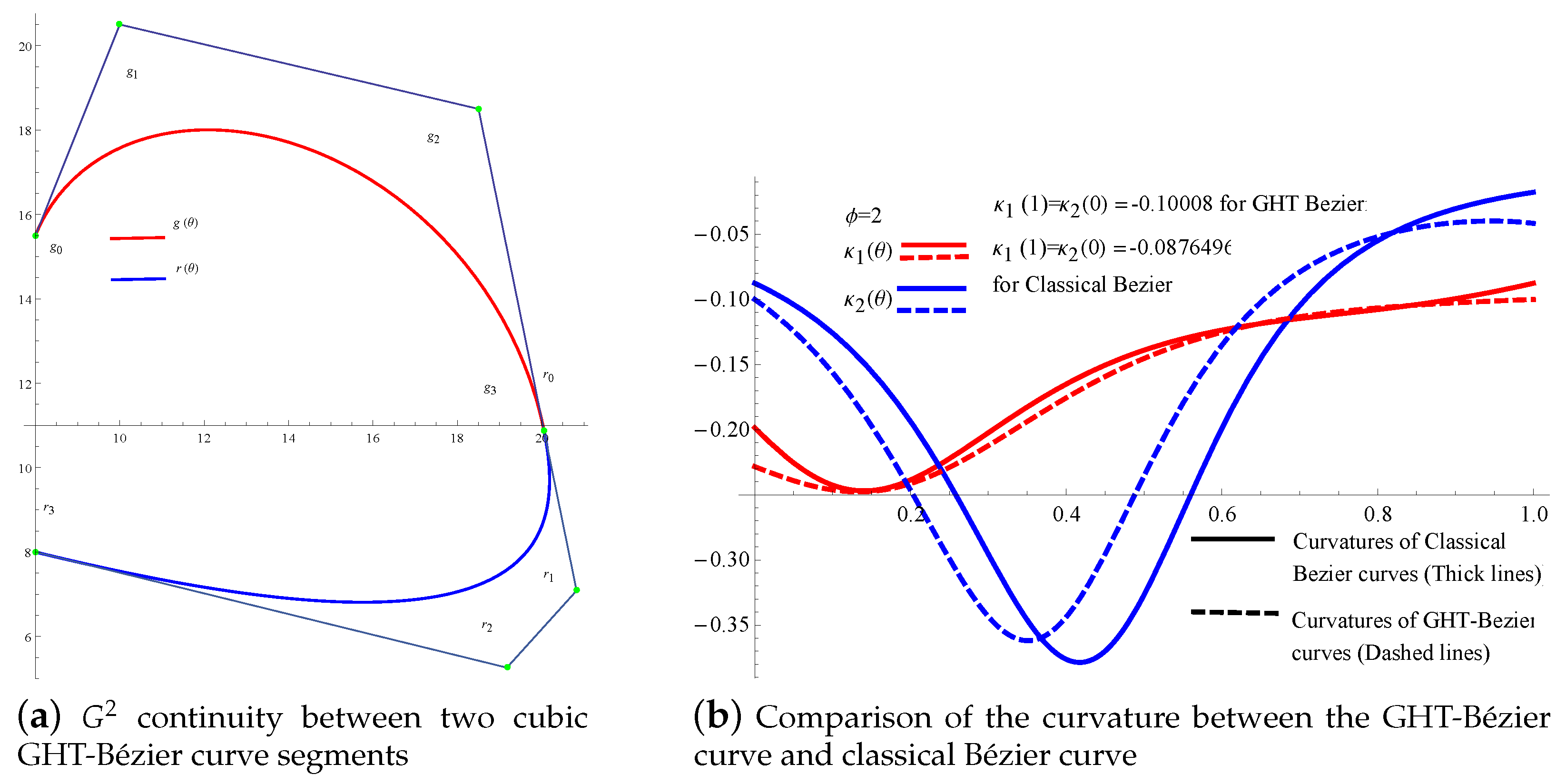
We already know that for the $G^0$ continuity condition, two curves meet with each other at joints, while for $G^1$ and $G^2$ continuity conditions, both curves (first and second) had the same tangent and curvature at the final and initial points, respectively. Similarly, for the $G^3$ continuity condition, the derivative of the curvature of both curves at the final and initial points was the same. Let us consider any two cubic GHT-Bézier curves $g\left(\theta \right)={\sum }_{i=0}^n{g}_i^{*}{q}_{i,n}\left(\theta \right)$ and $r\left(\theta \right)={\sum }_{i=0}^n{r}_i^{*}{q}_{i,n}\left(\theta \right)$. The curve $g\left(\theta \right)$ has the control points $g_0^{*}=(8,15.5)$, $g_1^{*}=(10,20.5)$, $g_2^{*}=(18.5,18.5)$, and $g_3^{*}=(20.05,10.89)$, while the curve $r\left(\theta \right)$ can be obtained by the $G^2$ continuity condition given in Theorem 4. The control point $r_3^{*}=(8,8)$ can be taken according to our own choice. It is also mentioned in Theorem 4 that the curvature of the first curve at the final point and the curvature of the second curve at initial point are the same.

Here, in Figure 12a, the red and blue curves are connected with each other by $G^2$ continuity, while in Figure 12b, the comparison of the curvature by the GHT-Bézier curve and classical Bézier curve is given. The solid lines represent the curvature of the classical Bézier curve, while dashed lines represent the curvature of the GHT-Bézier curve. The curvature values for the classical Bézier curve and GHT-Bézier curve are given in

Table 1. Curvature values for $G^2$ continuity by the classical Bézier curve.

$\mathit{\theta }$	Curvature ${\mathit{\kappa }}_1\left(\mathit{\theta }\right)$ (for Red Curve)	Curvature ${\mathit{\kappa }}_2\left(\mathit{\theta }\right)$ (for Blue Curve)
0	$-0.198502$	$-\mathbf{0.0876496}$
$0.1$	$-0.242583$	$-0.125836$
$0.2$	$-0.238606$	$-0.193501$
$0.3$	$-0.202376$	$-0.295431$
$0.4$	$-0.165009$	$-0.37619$
$0.5$	$-0.138967$	$-0.326819$
$0.6$	$-0.123578$	$-0.198955$
$0.7$	$-0.114671$	$-0.104602$
$0.8$	$-0.107853$	$-0.0549636$
$0.9$	$-0.0994784$	$-0.0303936$
1	$-\mathbf{0.0876496}$	$-0.178419$

and

Table 2. Curvature values for $G^2$ continuity by the GHT-Bézier curve.

$\mathit{\theta }$	Curvature ${\mathit{\kappa }}_1\left(\mathit{\theta }\right)$ (for Red Curve)	Curvature ${\mathit{\kappa }}_2\left(\mathit{\theta }\right)$ (for Blue Curve)
0	$-0.228373$	$-\mathbf{1.0008}$
$0.1$	$-0.246228$	$-0.156137$
$0.2$	$-0.241362$	$-0.246303$
$0.3$	$-0.212292$	$-0.343455$
$0.4$	$-0.175553$	$-0.343828$
$0.5$	$-0.145325$	$-0.23556$
$0.6$	$-0.125209$	$-0.135007$
$0.7$	$-0.113296$	$-0.0788477$
$0.8$	$-0.106581$	$-0.0519528$
$0.9$	$-0.102661$	$-0.0410629$
1	$-\mathbf{1.0008}$	$-0.0416751$

, respectively. It is obvious from the tables that the curvature values for the first (red) curve at the final point and the second (blue) curve at the initial point are identical i.e, (for classical Bézier curve the curvature values are identical as ${\kappa }_1\left(1\right)={\kappa }_2\left(0\right)=-\mathbf{0.0876496}$, while for GHT-Bézier curve the values of curvature are identical as ${\kappa }_1\left(1\right)={\kappa }_2\left(0\right)=-\mathbf{1.0008}$) and it can also be deduced that the curves preserve the curvature continuity from one curve to another.

6. Curvature Junction of GHT-Bézier Curves by ${\mathit{G}}^{\mathbf{3}}$ Continuity

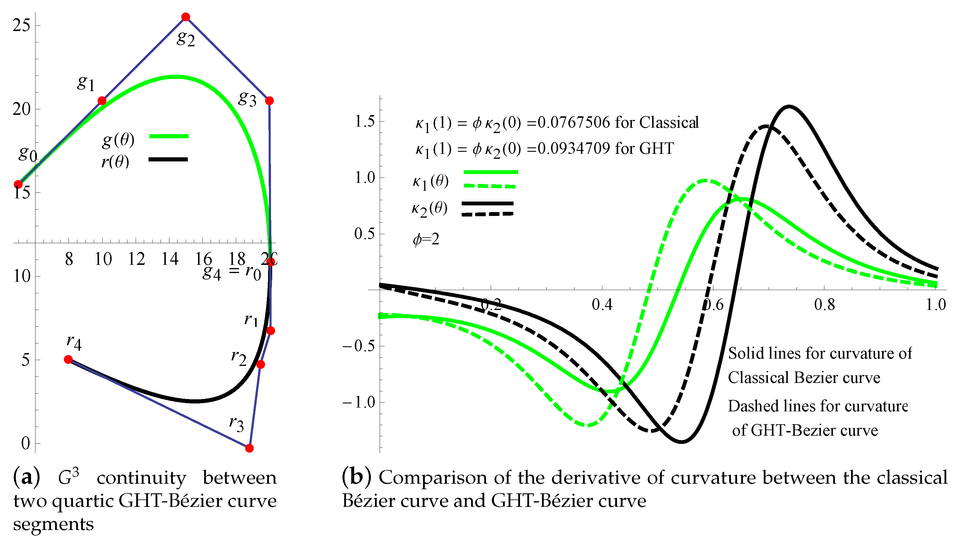
As we are already familiar with the fact that the conventional $C^k$ continuity cannot provide us with an extra parameter, $G^k$ continuity provides us an additional parameter for further optimization. Just like $G^2$ continuity behaves as curvature continuity, $G^3$ continuity represents the derivative of curvature continuity. For $G^3$ continuity conditions, the derivative of the curvature of the first curve at the final point and the derivative of the curvature of the second curve at the initial point will be the same, i.e., ${\kappa }_1^{{}^{\prime }}\left(1\right)=\varphi {\kappa }_2^{{}^{\prime }}\left(0\right).$ Consider any two quartic GHT-Bézier curves named as $g\left(\theta \right)$ and $r\left(\theta \right)$, respectively. The control points of the first curve are given as $g_0^{*}=(5,15.5)$, $g_1^{*}=(10,20.5)$, $g_2^{*}=(15,25.5)$, $g_3^{*}=(20,20.5)$, and $g_4^{*}=(20.05,10.89)$, while the control points of the second curve were obtained by using $G^3$ continuity conditions described in Theorem 4, and the last control point was $r_4^{*}=(8,5)$. Here, in Figure 13a, the green and black curves are joined by $G^3$ continuity conditions, while in Figure 13b, the comparison of the derivative of curvature by the classical Bézier curve and GHT-Bézier curve is given. The solid and dashed lines represent the derivative of the curvature of the classical Bézier curve and GHT-Bézier curve, respectively. It is obvious from Figure 13 and

Table 3. Curvature values for $G^3$ continuity by the classical Bézier curve.

$\mathit{\theta }$	Values of ${\mathit{\kappa }}_1^{{}^{\prime }}\left(\mathit{\theta }\right)$ (for Green Curve)	Values of ${\mathit{\kappa }}_2^{{}^{\prime }}\left(\mathit{\theta }\right)$ (for Black Curve)	Values of $\mathit{\varphi }{\mathit{\kappa }}_2^{{}^{\prime }}\left(\mathit{\theta }\right)$
0	$-0.212132$	$0.0467354$	$\mathbf{0.0934709}$
$0.1$	$-0.220298$	$-0.020342$	$-0.040684$
$0.2$	$-0.332911$	$-0.114935$	$-0.22987$
$0.3$	$-0.584367$	$-0.281849$	$-0.563698$
$0.4$	$-0.867004$	$-0.627451$	$-1.254902$
$0.5$	$-0.408314$	$-1.21847$	$-2.43694$
$0.6$	$0.680648$	$-0.850415$	$-1.70083$
$0.7$	$0.754765$	$1.42099$	$2.84198$
$0.8$	$0.420498$	$1.23211$	$2.46422$
$0.9$	$0.202457$	$0.499801$	$0.999602$
1	$\mathbf{0.0934709}$	$0.190699$	$0.381398$

and

Table 4. Curvature values for $G^3$ continuity by the GHT Bézier curve.

$\mathit{\theta }$	Values of ${\mathit{\kappa }}_1^{{}^{\prime }}\left(\mathit{\theta }\right)$ (for Green Curve)	Values of ${\mathit{\kappa }}_2^{{}^{\prime }}\left(\mathit{\theta }\right)$ (for Black Curve)	Values of $\mathit{\varphi }{\mathit{\kappa }}_2^{{}^{\prime }}\left(\mathit{\theta }\right)$
0	$-0.180035$	$0.0383753$	$\mathbf{0.0767506}$
$0.1$	$-0.233158$	$-0.0738331$	$-0.1476662$
$0.2$	$-0.442069$	$-0.211072$	$-0.422144$
$0.3$	$-0.894591$	$-0.459873$	$-0.919746$
$0.4$	$-1.09659$	$-0.921015$	$-1.84203$
$0.5$	$0.305785$	$-1.21166$	$-2.42332$
$0.6$	$1.00343$	$0.351962$	$0.703924$
$0.7$	$0.610066$	$1.45387$	$2.90774$
$0.8$	$0.296791$	$0.80677$	$1.61354$
$0.9$	$0.148436$	$0.324799$	$0.649598$
1	$\mathbf{0.0767506}$	$0.125541$	$0.1535012$

that the derivative of the curvature of the first curve at the final point and the second curve at the initial point is identical. For the classical Bézier curve, ${\kappa }_1^{{}^{\prime }}\left(1\right)=\varphi {\kappa }_2^{{}^{\prime }}\left(0\right)=\mathbf{0.0934709}$, while for the GHT-Bézier curve, ${\kappa }_1^{{}^{\prime }}\left(1\right)=\varphi {\kappa }_2^{{}^{\prime }}\left(0\right)=\mathbf{0.0767506}.$

Main Result

From the above discussion of curvature junction, we concluded that the GHT-Bézier curve was superior to the classical Bézier curve due to the significance that the curvature junction value for the GHT-Bézier curve could be changed as we varied the values of the shape parameter in their domain, but the curvature junction values for the classical Bézier curve always remained the same.

7. Applications

As an extension of the traditional Bézier curve, the GHT-Bézier curve provides a new way of mathematical theory for the excellence of CAGD and CAD. Its application range includes computer graphics, image processing, font designing, modeling of complex figures, computer vision, etc. If we need to design any complex shape by GHT-Bézier curves, then we must consider it as a piecewise curve composed of multiple ones. Those piecewise curves will be worthier if we join them by using various continuity conditions as given in Figure 14 and Figure 15. In recent years, we have seen beautiful buildings and roads constructed by using computer technology. Therefore, currently, we can compose multiple maps of buildings, bridges, highway designs, and also sketching and various designing by the help of GHT-Bézier curves, which are very useful in daily life. As font designing and sketching are difficult to fit due to having various curves and cusps, as an application of continuity conditions, the construction of multiple complex figures is given below.

Construction of Free-Form Complex Figures by Parametric and Geometric Continuity Constraints

In order to resolve the problem of the construction of complex figures (which cannot be executed by a single curve), the $C^3$ and $G^3$ continuity conditions were derived. Since GHT-Bézier curves are capable of designing any curve of n degrees, by using any two adjacent GHT-Bézier curves having the same degrees and the above continuity conditions, multiple shapes can be constructed.

Example 9.

In Figure 14a–c, a beautiful graph of a fish is composed by using two adjacent quartic Bézier curves, which meets the $C^1$ continuity conditions.

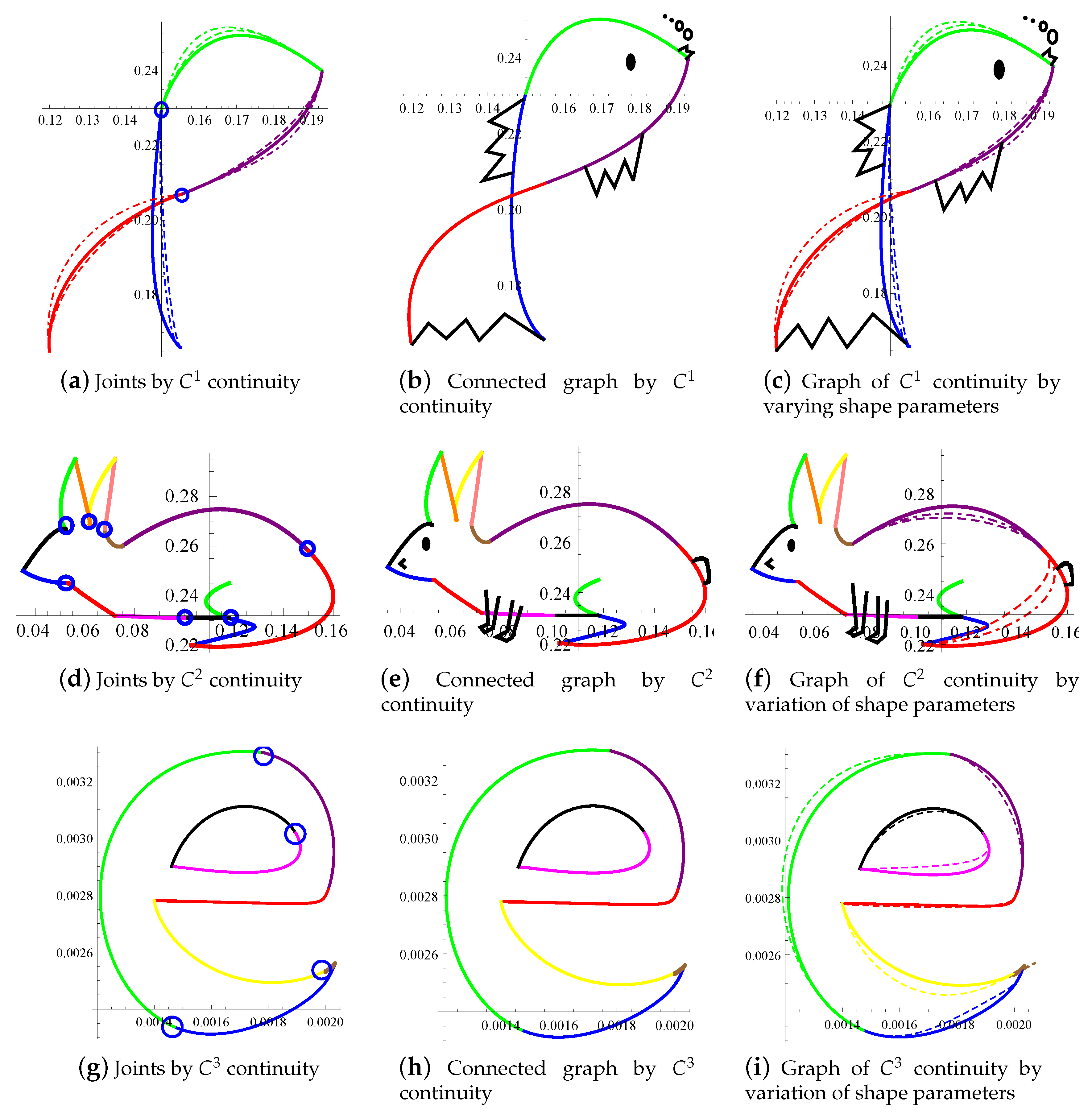
Here, the green curve is obtained by using the initial curve having the control points $P_0^{*}=(0.193,0.24)$, $P_1^{*}=(0.176,0.253)$, $P_2^{*}=(0.158,0.26)$, $P_3^{*}=(0.15,0.23)$, and $P_4^{*}=(0.15,0.23)$, while the blue curve is obtained by the $C^1$ continuity condition given in Equation (11). Here, the control points $Q_2^{*}=(0.147,0.173)$, $Q_3^{*}=(0.155,0.166)$, and $Q_4^{*}=(0.155,0.166)$ of the second curve are adjusted according to our own will. Similarly, the purple curve is constructed by using the initial quartic Bézier curve, and the red curve is attained when we met the continuity conditions. Here, in Figure 14a, the blue circle shows the joint point between the initial and final curve (obtained by $C^1$ continuity), while in Figure 14c, the dashed and dotted-dashed curves are obtained by varying multiple shape parameters in their domain. Figure 14d–f presents the most complex graph of a rabbit by joining various segments obtained by the continuity constraints of GHT-Bézier curves. This graph also ensures that the GHT-Bézier curves have the capability to construct any complex figure as we desired. Here, in Figure 14d, the blue circle shows the joint point between two GHT-Bézier curves connected by $C^2$ continuity constraints. Similarly, Figure 14e shows the complete graph of the GHT-Bézier curve, while in Figure 14f, the multi-colored dashed and dashed-dotted lines are obtained by varying the multiple shape parameters in their given domain. Just like the $C^1$ and $C^2$ continuity conditions, we can also construct various complex figures with great smoothness by using the $C^3$ continuity conditions of the GHT-Bézier curves. In Figure 14g–i, the graph of the English letter e is presented. In Figure 14g, multiple curves are joined to make the smooth graph, and the joint points are highlighted with tiny blue circles. Figure 14h presents the complete figure, while Figure 14i shows the beautiful figure with dashed lines, which have been obtained by varying the multiple shape parameters.

Example 10.

It is well known that in geometric continuity, the tangents are collinear, and they may not have the same magnitude, while in parametric continuity, the magnitudes of the vectors are always equal. Due to these distinctions, the curves obtained by geometric continuity have more smoothness as compared to the curves obtained by parametric continuity.

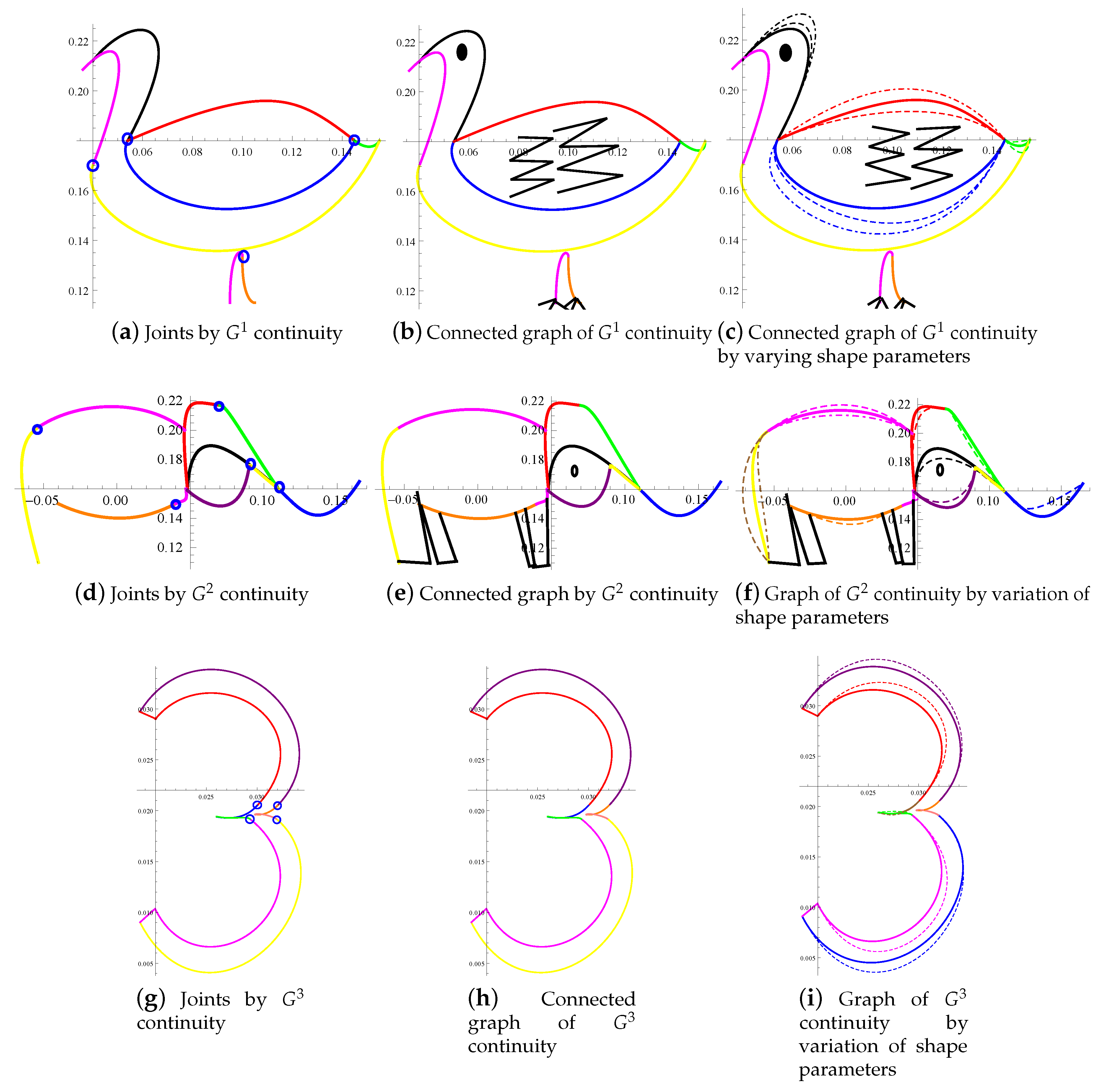
Figure 15 displays the disparate shapes constructed by $G^1$, $G^2$, and $G^3$ continuity conditions. In Figure 15a, a beautiful shape of a duck is constructed by $G^1$ continuity constraints. The blue circles in this figure highlight the junction between the two curves (initial curve and the curve obtained after applying continuity conditions). Similarly, Figure 15b shows the spliced graph of a duck, while the variation in curves by varying the shape parameters can be seen in Figure 15c as dashed and dashed-dotted lines.

The shape of an elephant wasis constructed by using $G^2$ continuity conditions. Just like Figure 15a, the tiny blue circles demonstrate the continuity conditions between the initial and final curve (the curve obtained after continuity conditions) segments given in Figure 15d. The very next figure gives us the splicing graph of the elephant obtained by $G^2$ continuity and Figure 15e shows the spliced graph. The dashed and dashed-dotted lines demonstrate the variation in the values of the shape parameters.

After $G^1$ and $G^2$ continuity conditions, now we turn to construct any figure by using $G^3$ continuity conditions to show the efficiency of GHT-Bézier curves in modeling and shape preserving processes. Here, in Figure 15g–i, the modeling of a natural number three is presented by using $G^3$ continuity conditions, which shows that sketching and modeling can also be possible by using GHT-Bézier curves with the continuity constraints. In Figure 15g, the blue circles show the joint points of the initial and final curves. Here, four different curves are joined with each other and compiled in Figure 15h. In Figure 15i, the dashed curves are obtained by varying multiple shape parameters. The control points for all these figures are mentioned as follows. In this figure, the continuity conditions between the magenta curve of degree three and the green curve of degree four are presented. For the magenta curve, the control points are $P_0^{*}=(0.02,0.0103)$, $P_1^{*}=(0.02,0.0103)$, $P_2^{*}=(0.039,0.0115)$, and $P_3^{*}=(0.0293,0.01918)$, while the first three control points of the green curve are obtained by continuity conditions, and the last control point is adjusted by our own choice and taken as $Q_4^{*}=(0.026,0.0194)$. The shape parameters can also be adjusted to obtain the desired curve. Similarly, yellow, red, and purple curves are the initial curves, while pink, blue, and orange curves are obtained by using continuity conditions. Their control points are adjusted to obtain the required shape. Finally, by joining all these curves, we obtained a perfect shape of a natural number three. To beautify this shape, we altered the values of the shape parameters in their domain and obtained a beautiful graph given in Figure 15i.

8. Conclusions

We know that GHT-Bézier curves, as well as classical Bézier curves are very useful for image processing, graphics, and font designing. By using two points, we can only draw a straight line. However, as we increase the number of control points, we can obtain any curved shape. However, when we talk about the modeling of complex figures and font designing, only a single GHT-Bézier curve is not sufficient. To solve this issue, the parametric and geometric continuity conditions up to degree three ($C^3$ and $G^3$ continuity) between any two GHT-Bézier curves were derived in this research paper. The curvature junction by using the $G^2$ and $G^3$ continuity of GHT-Bézier curves and classical Bézier curves was also discussed. Further, we mentioned the parametric and geometric continuity conditions of GHT-Bézier curves along with curvature junction. However, the new approach given in this research paper was the derivation of the $G^3$ continuity condition for geometric modeling of complex figures, and as far as we are aware, it has never been employed for this purpose before.

Moreover, by using ($C^3$ and $G^3)$ continuity conditions, we mentioned some useful applications by the construction of some complex figures and font designing as well. The variation in the figures with multiple shape parameters was also given. The technique proposed in this study could develop curves whose mathematical complication is not increased, which makes it more useful in practical applications. Some curve design examples exhibited that this scheme was more convenient, flexible, and effective for both curve and surface interaction modeling and had significant mathematical and applied applications. Additionally, this scheme could be applied in the future to generate trigonometric surfaces over triangles with multiple shape parameters.

References

- Wan Nurhadani, W.J.; Piah, A.R.M.; Abbas, M. Shape Preserving Visualization of Monotone Data using Rational Cubic Ball Function. Sci. Asia 2014, 40S, 40–46. [Google Scholar] [CrossRef] [Green Version]
- Abbas, M.; Majid, A.A.; Ali, J.M. Monotonicity-Preserving C2 Rational Cubic Spline for Monotone Data. Appl. Math. Comput. 2012, 219, 2885–2895. [Google Scholar]
- Abbas, M.; Majid, A.A.; Awang, M.N.H.; Ali, J.M. Positivity-Preserving C2 Rational Cubic Spline Interpolation. Sci. Asia 2013, 39, 208–213. [Google Scholar] [CrossRef] [Green Version]
- Abbas, M.; Majid, A.A.; Ali, J.M. Positivity-preserving rational bi-cubic spline interpolation for 3D positive data. Appl. Math. Comput. 2014, 234, 460–476. [Google Scholar] [CrossRef]
- Abbas, M.; Majid, A.A.; Awang, M.N.H.; Ali, J.M. Monotonicity Preserving Rational Bi-Cubic Spline Surface Interpolation. Sci. Asia 2014, 40S, 22–30. [Google Scholar] [CrossRef] [Green Version]
- Abbas, M.; Majid, A.A.; Awang, M.N.H.; Ali, J.M. Convexity Preserving Rational Bi-Cubic Spline Surface Interpolation. Sci. Asia 2014, 40S, 31–39. [Google Scholar] [CrossRef] [Green Version]
- Hering, L. Closed (C2 and C3 continuous) Bézier and B-spline curves with given tangent polygons. Comput. Aided Des. 1983, 15, 3–6. [Google Scholar] [CrossRef]
- Yan, L. Adjustable Bézier Curves with Simple Geometric Continuity Conditions. Math. Comput. Appl. 2016, 21, 44. [Google Scholar] [CrossRef] [Green Version]
- Schneider, R.; Kobbelt, L. Discrete fairing of curves and surfaces based on linear curvature distribution. Curve Surface Des. 1999, 1999, 371–380. [Google Scholar]
- Barsky, B.A.; Derose, T.D. Geometric continuity of parametric curves: Three equivalent characterizations. IEEE Comput. Graph. Appl. 1989, 9, 60–69. [Google Scholar] [CrossRef]
- Hu, G.; Bo, C.; Wu, J.; Wei, G.; Hou, F. Modeling of free-form complex curves using SG-Bézier curves with constraints of geometric continuities. Symmetry 2018, 10, 545. [Google Scholar] [CrossRef] [Green Version]
- Bashir, U.; Abbas, M.; Ali, J.M. The G2 and C2 rational quadratic trigonometric Bézier curve with two shape parameters with applications. Appl. Math. Comput. 2013, 219, 10183–10197. [Google Scholar] [CrossRef]
- Usman, M.; Abbas, M.; Miura, K.T. Some engineering applications of new trigonometric cubic Bézier-like curves to free-form complex curve modeling. J. Adv. Mech. Des. Syst. Manuf. (Des. Syst.) 2020, 14, 1–15. [Google Scholar] [CrossRef] [Green Version]
- Qin, X.; Hu, G.; Zhang, N.; Shen, X.; Yang, Y. A novel extension to the polynomial basis functions describing Bézier curve and surfaces of degree n with the multiple shape parameters. Appl. Math. Comput. 2013, 223, 1–16. [Google Scholar] [CrossRef]
- BiBi, S.; Abbas, M.; Misro, M.Y.; Hu, G. A novel approach of hybrid trigonometric Bézier curve to the modeling of symmetric revolutionary curves and symmetric rotation surfaces. IEEE Access 2019, 7, 165779–165792. [Google Scholar] [CrossRef]
- Misro, M.Y.; Ramli, A.; Ali, J.M. Quintic Trigonometric Bézier curve with two shape parameters. Sains Malaysiana 2017, 46, 825–831. [Google Scholar]
- Veltkamp, R.C. Survey of continuities of curves and surfaces. Comput. Graph. Forum 1992, 11, 93–112. [Google Scholar] [CrossRef] [Green Version]
- Hu, G.; Cao, H.; Qin, X.; Wang, X. Geometric design and continuity conditions of developable λ-Bézier surfaces. Adv. Eng. Softw. 2017, 114, 235–245. [Google Scholar] [CrossRef]
- Farin, G. Curves and Surfaces for CAGD. A Practical Guide, 5th ed.; Academic Press: San Diego, CA, USA, 2002. [Google Scholar]
- Liu, H.; Li, L.; Zhang, D.; Wang, H. Cubic Trigonometric Polynomial B-spline curve and surfaces with shape parameter. J. Inf. Comput. Sci. 2012, 9, 989–996. [Google Scholar]
- Dube, M.; Yadav, B. The quintic trigonometric Bézier curve with single shape parameter. Int. J. Sci. Res. Publ. 2014, 4, 2250–3153. [Google Scholar]
- Sharma, R.; Dube, M. Shape Features of Cubic Trigonometric Bézier Curve With Two Shape Parameters. Proc. Natl. Conf. Pure Appl. Math. 2015, 2015, 13–17. [Google Scholar]
- Dube, M.; Sharma, R. Quartic Trigonometric Bézier curve with a shape parameter. Int. J. Math. Comput. Appl. Res. 2013, 3, 89–96. [Google Scholar]
- Papp, I.; Hoffmann, M. C2 and G2 continuous spline curves with shape parameters. J. Geom. Graph. 2007, 11, 179–185. [Google Scholar]
- Qin, X.; Hu, G.; Shen, X. Shape modification of Quartic C-Bézier curves. Comput. Eng. Appl. 2014, 50, 178–181. [Google Scholar]
- Han, X.; Ma, Y.; Huang, X. The cubic trigonometric Bézier curve with two shape parameters. Appl. Math. Lett. 2009, 22, 226–231. [Google Scholar] [CrossRef] [Green Version]
- Hu, G.; Wu, J.; Qin, X. A novel extension of the Bézier model and its applications to surface modeling. Adv. Eng. Softw. 2018, 125, 27–54. [Google Scholar] [CrossRef]
- Sharma, R. A Class of QT Bézier Curve with Two Shape Parameters. Int. J. Sci. Res. 2016, 5, 131–134. [Google Scholar]
- Bashir, U.; Abbas, M.; Hj Awang, M.N.; Md. Ali, J. A Class of quasi-quintic trigonometric Bézier curve with two shape parameters. Sci. Asia 2013, 39, 11–15. [Google Scholar] [CrossRef] [Green Version]
- Yang, L.; Li, J.; Chen, G. A Class of quasi-quartic trigonometric Bézier curves and surfaces. J. Inf. Comput. Sci. 2012, 7, 72–80. [Google Scholar]
- Wu, X.; Han, X.; Luo, S. Quadratic trigonometric spline curve with multilpe shape parameters. IEEE Int. Conf. Comput. Aided Des. Comput. Graph. 2007, 3–6. [Google Scholar] [CrossRef]
- Shen, W.Q.; Wang, G.H. Geometric shapes of C-Bézier curves. Comput. Aided Geom. Des. 2015, 58, 217–242. [Google Scholar] [CrossRef]
- Mainer, E. Shape preserving alternatives to the rational Bézier model. Comput. Aided Geom. Des. 2001, 18, 37–60. [Google Scholar] [CrossRef]
- Liang, X. Bernstein Bézier class curves and a representation method of Bézier curve. J. Comput. Res. Dev. 2004, 41, 1016–1021. [Google Scholar]
- Liu, Z.; Chen, X.; Jiang, P. A class of generalized Bézier curves and surfaces with multiple shape parameters. J. Comput. Aided Des. Comput. Graph. 2010, 22, 838–844. [Google Scholar] [CrossRef]
- Han, X.; Ma Chen, L.; Huang, X. A novel generalization of curve and surface. J. Comput. Appl. Math. 2008, 217, 180–193. [Google Scholar] [CrossRef] [Green Version]
- Qin, X.; Hu, G.; Yang, Y.; Wei, G. Construction of PH splines based on H-Bézier curves. Appl. Math. Comput. 2014, 238, 460–467. [Google Scholar] [CrossRef]
- Wang, A.; Zhao, G.; Hou, F. Constructing Bézier curves with monotone curvature. J. Computat. Appl. Math. 2019, 355, 1–10. [Google Scholar] [CrossRef]
- Yahya, F.; Ali, M.J.; Ibrahim, A.; Majid, A.A. An Automatic Generation of G1 Curve Fitting of Arabic Chracters. In Proceedings of the International Conference on Computer Graphics, Imaging and Visualisation (CGIV’06), Sydney, QLD, Australia, 26–28 July 2006. [Google Scholar]
- Wang, W.T.; Wang, G.Z. Bézier curve with shape parameter. J. Zhejiang Univ. Sci. 2005, 6A, 497–501. [Google Scholar]
- Han, A.X.; Huang, X.L.; Ma, C.Y. Shape analysis of Cubic Trigonometric Bézier curve with the shape parameter. Appl. Math. Comput. 2010, 217, 2527–2533. [Google Scholar] [CrossRef]
- Hu, G.; Bo, C.C.; Qin, X.Q. Continuity conditions for Q-Bézier curves of degree n. J. Inequal. Appl. 2017, 115, 1–14. [Google Scholar] [CrossRef] [Green Version]
- Pelosi, F.; Farouki, R.T.; Manni, C.; Sestini, A. Geometric Hermite interpolation by spatial Pythagorean-hodograph cubics. Adv. Comput. Math. 2005, 22, 325–352. [Google Scholar] [CrossRef]
- Ait-Haddou, R.; Barton, M. Constrained multi-degree reduction with respect to Jacobi norms. Comput. Aided Geom. Des. 2016, 42, 23–30. [Google Scholar] [CrossRef] [Green Version]
- González, C.; Albrecht, G.; Paluszny, M.; Lentini, M. Design of C2 algebraic-trigonometric Pythagorean hodograph splines with shape parameters. Comp. Appl. Math. 2016, 378, 1472–1495. [Google Scholar]
Figure 1.
GHT-Bernstein basis functions of various degrees. (a) Quartic HT-Bernstein basis function; (b) quintic HT-Bernstein basis function; (c) hexic HT-Bernstein basis function; (d) nonic HT-Bernstein basis function.
Figure 2.
Cubic HT-Bézier curves with distinct shape parameters. (a) (b) (c) (d)
Figure 3.
Shape control of GHT-Bézier curves with distinct shape parameters. (a) ; (b) ; (c) ; (d) .
Figure 4.
continuity of the GHT-Bézier curve by multi-valued shape parameters. (a) : ; (b) : ; (c) : ; (d) : .
Figure 5.
Graphical representation of the continuity of the GHT-Bézier curve. (a) : ; (b) : ; (c) : ; (d) : .
Figure 6.
Graphical representation of the continuity of the GHT-Bézier curve by various shape parameters. (a) : ; (b) : ; (c) : ; (d) : .
Figure 7.
and continuity between GHT-Bézier curves having different degrees. (a) continuity between cubic and quartic GHT-Bézier curves; (b) continuity between cubic and quartic GHT-Bézier curves.
Figure 8.
smooth continuity of the GHT-Bézier curve with multiple shape parameters. (a) : ; (b) : ; (c) : ; (d) : .
Figure 9.
smooth continuity of the GHT-Bézier curve with various shape parameters. (a) : ; (b) : ; (c) : ; (d) : .
Figure 10.
Figure 11.
Geometric continuity between two GHT-Bézier curves of different degrees. (a) continuity between two GHT-Bézier curves of different degrees; (b) continuity between two GHT-Bézier curves of different degrees.
Figure 12.
Graphical representation of the continuity for the GHT-Bézier curve and the classical Bézier curve. (a) continuity between two cubic GHT-Bézier curve segments; (b) comparison of the curvature between the GHT-Bézier curve and classical Bézier curve.
Figure 13.
Graphical representation of the continuity for the GHT-Bézier curve and classical Bézier curve. (a) continuity between two quartic GHT-Bézier curve segments; (b) comparison of the derivative of curvature between the classical Bézier curve and GHT-Bézier curve.
Figure 14.
Modeling by the , , and smooth continuity of GHT-Bézier curves by varying shape parameters. (a) Joints by continuity; (b) connected graph by continuity; (c) graph of continuity by varying shape parameters; (d) joints by continuity; (e) connected graph by continuity; (f) graph of continuity by variation of shape parameters; (g) joints by continuity; (h) connected graph by continuity; (i) graph of continuity by variation of shape parameters.
Figure 15.
Modeling of complex figures by , , and smooth continuity, respectively, of GHT-Bézier curves with multiple shape parameters. (a) Joints by continuity; (b) connected graph of continuity; (c) connected graph of continuity by varying shape parameters; (d) joints by continuity; (e) connected graph by continuity; (f) graph of continuity by variation of shape parameters; (g) joints by continuity; (h) connected graph of continuity; (i) graph of continuity by variation of shape parameters.