
Water Regulation Ecosystem Services of Multifunctional Landscape Dominated by Monoculture Plantations
by
 , ,
, ,
Yudha Kristanto
1,2,* ,
,
Suria Tarigan
3,
Tania June
4,
Enni Dwi Wahjunie
3 and
Bambang Sulistyantara
5 1
Watershed Management Science, Department of Soil Science and Land Resources Management, Faculty of Agriculture, IPB University, Bogor 16680, Indonesia
2
Natural Resources and Environmental Management Science, Graduate School, IPB University, Bogor 16129, Indonesia
3
Department of Soil Science and Land Resources Management, Faculty of Agriculture, IPB University, Bogor 16680, Indonesia
4
Department of Geophysics and Meteorology, Faculty of Mathematics and Natural Sciences, IPB University, Bogor 16680, Indonesia
5
Department of Landscape Architecture, Faculty of Agriculture, IPB University, Bogor 16680, Indonesia
*
Author to whom correspondence should be addressed.
Land 2022, 11(6), 818; https://doi.org/10.3390/land11060818
Submission received: 2 April 2022
/
Revised: 25 May 2022
/
Accepted: 28 May 2022
/
Published: 31 May 2022
(This article belongs to the Special Issue Soil Management for Sustainable Agriculture and Ecosystem Services)
Abstract
:Meeting the growing demand for agricultural production while preserving water regulation ecosystem services (WRES) is a challenge. One way to preserve WRES is by adopting multifunctional landscape approach. Hence, the main objective was to evaluate the role of forest patches (FP) in preserving WRES in tropical landscapes dominated by oil palm plantations. The SWAT model was used to evaluate the essential WRES, such as water yield (WYLD), soil water (SW), surface runoff (SURQ), groundwater recharge (GWR), and evapotranspiration (AET). Due to a compaction, soils in monoculture plantation have higher bulk density and lower porosity and water retention, which decrease WRES. Conserving FP among oil palms evidently improves WRES, such as decreasing SURQ and rain season WYLD and increasing GWR, SW, AET, and dry season WLYD. FP has sponge-like properties by storing water to increase water availability, and pump-like properties by evaporating water to stabilize the microclimate. Mature oil palm also has pump-like properties to maintain productivity. However, it does not have sponge-like properties that make water use more significant than the stored water. Consequently, a multifunctional landscape could enhance WRES of forest patches and synergize it with provisioning ecosystem services of oil palm plantations.
1. Introduction
Local, countrywide, and global consumption of processed palm oil products, such as food, bioenergy, and oleochemicals, is growing along with population growth. This phenomenon implies changing the tropical landscapes into oil palm plantations (Elaeis guineensis Jacq.) that are intensively cultivated in monocultures [1]. The area of oil palm plantations has rapidly grown and is expected to increase in the coming years [2,3]. On the one hand, the development of oil palm plantations rapidly contributes to the local, regional, and national economies [4]. In addition, oil palm plantations also positively impact increasing access to the basic needs of local communities, such as school facilities, health facilities, road networks, and electricity networks. However, if the development of oil palm plantations is not appropriately managed, it can cause the degradation of ecosystem services, and reduce the ecological function of a landscape and harms the socio-economic community [5].
Previous research has examined the transformation of natural ecosystem into agroecosystem, especially monoculture plantations on ecosystem services changes [2]. One of the noticeable changes in ecosystem services in agroecosystem is the change in water regulation ecosystem services (WRES) caused by soil compaction due to intensive land management. These phenomena encompass a decrease in infiltration [6], an increase in surface runoff in the rainy season [3], and a decrease in groundwater availability in the dry season [5]. Therefore, meeting the growing demand for oil palm production while maintaining WRES is a challenge faced by a landscape of oil palm plantations related to sustainable and climate smart agriculture. Ecosystem services support human well-being through provision, regulation, and culture formed by natural and manufactured ecosystem structures and processes. WRES are essential ecosystem services in sustainable development, referring to the quantity, quality, and time of water stored in and out of an ecosystem [7]. WRES benefits are freshwater supply, flood and drought protection, electrical power generation, irrigation, and aquatic ecosystem maintenance.
One way to balance landscape WRES is by applying a multifunctional landscape approach through preserving the remnants of forest patches among oil palm plantations. These forest patches can be in secondary dryland forests, riparian vegetation, or agroforestry systems designated as high conservation areas (HCV). A multifunctional landscape is a landscape that can serve multiple ecosystem services simultaneously, not only for provisioning services, but also for regulation, cultural, and support services [8]. The multifunctional landscape is a more realistic soil and water conservation approach to optimize ecosystem services, where forest patches serve water regulation and the other regulation services, while oil palm plantations serve crop production. Furthermore, the multifunctional landscape maps the potential trade-offs and win-win synergies between each ecosystem service, especially provisioning services, which often conflict with regulation, cultural, and support services [9].
Since forest patches are essential to maintain the balance of landscape-scale WRES, it is necessary to model and evaluate WRES on oil-palm-dominated landscapes assisted by dynamic models, such as the Soil and Water Assessment Tools (SWAT). The strength of SWAT in WRES simulation is that SWAT has complex parameters and model structures, which can simulate the influence of physical processes in the soil–plant–atmosphere continuum that affects WRES on the watershed scale. However, field observation cannot measure several SWAT parameters, so the uncertainty that arises from parameter justification needs to be evaluated and considered in selecting the output model to be interpreted. In addition, previous research on oil palm ecosystem services generally does not differentiate between mature and young oil palms, especially in the same tropical landscape [3,6]. Oil palm growths affect the WRES changes through soil compaction due to intensive cultivation activities and canopy development that affect hydrological parameters at the hydrologic response unit (HRU) scale.
Because of soil compaction, WRES evaluation in this study needs to consider the soil hydrological characteristics and soil water retention curve (SWRC) at the smallest analysis unit, which significantly affect the WRES due to different land use and crop dynamics. The relationship between SWRC and WRES occurs at the HRU scale, where the information from SWRC is inputted into the .sol database to update the HRU value. SWRC was closely related to calculating the retention parameter of curve number and the range of soil moisture dynamics that affect surface runoff, evapotranspiration, and soil water storage. When the HRU as the smallest unit of analysis is updated, the sub-basin parameters are automatically updated through the routing mechanism. Therefore, this study answers the main research question: how do forest patches preserve WRES in landscapes dominated by oil palm plantations? Consequently, two objectives can be drawn in this study: (i) analyze the soil water retention characteristics of each land use due to land management, and (ii) evaluate the role of forest patches among oil palm plantations in preserving landscape-scale WRES.
2. Materials and Methods
2.1. Study Area
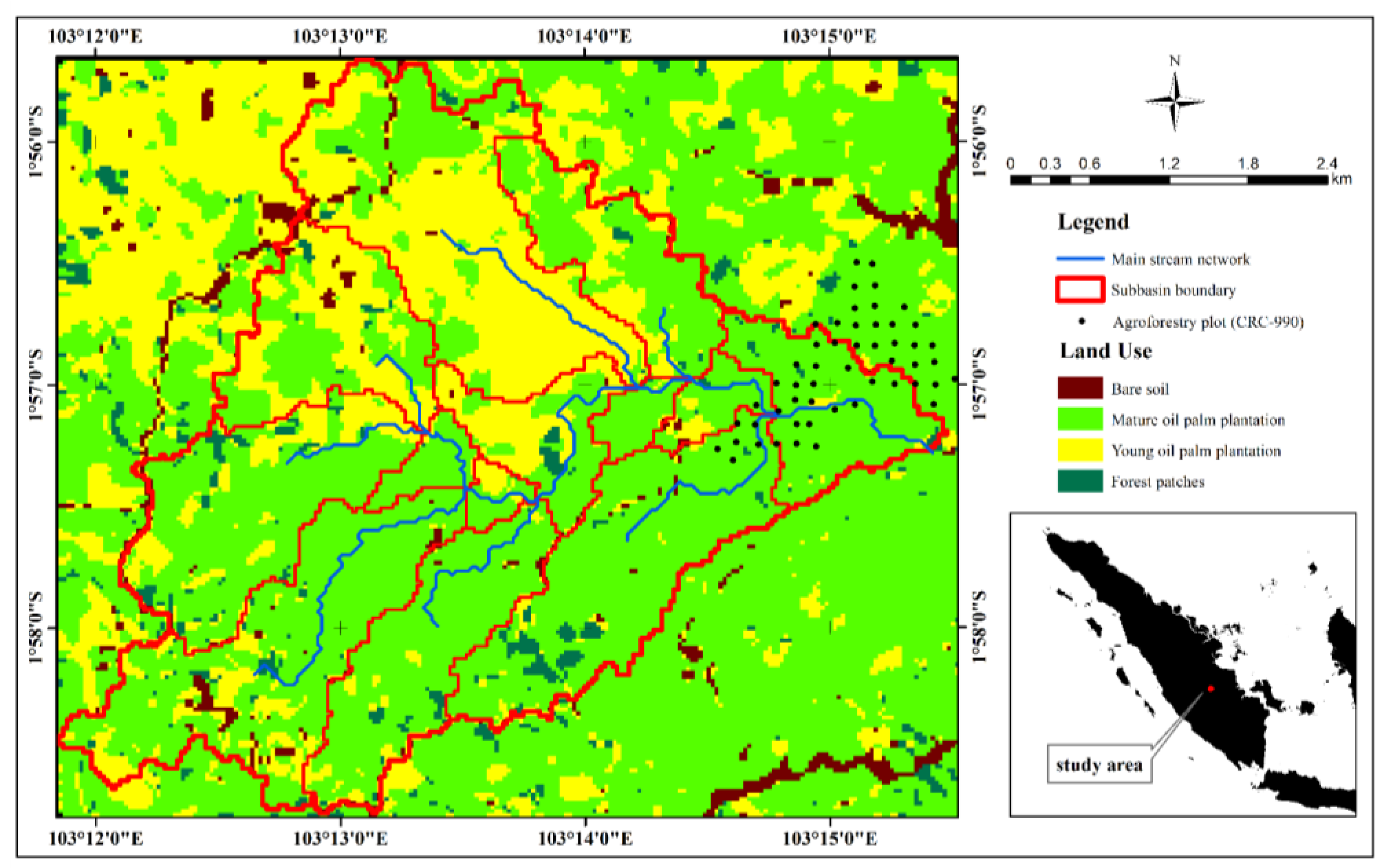
The study area is a tropical lowland located in Jambi Province, Sumatra, Indonesia. This area has an equatorial rainfall type, characterized by two peaks of the rainy season (December and April) and one dry season (July) in one year. This area also has the same soil type, Hapludults, with a sandy clay loam texture (50% sand, 30% clay, and 20% silt) with small topography variations. The land use is dominated by oil palm plantations that are cultivated in monoculture, both mature plants (MOP) and young plants (YOP) (Figure 1). Among oil palm plantations, there are remnants of forest patches (FP) in the form of secondary dryland forest, riparian vegetation, and agroforestry plot separated from their primary ecosystem. The agroforestry plot (AGF ex-MOP) was planted in 2013 from former mature oil palm plantations.
A micro-watershed with 13 sub-basins is delineated as a system boundary for WRES modeling. The micro-watershed has an area of 19.1 square kilometers, and lies between 1°55′38.7″–1°58′48.3″ S and 103°11′50.1″–103°15′34.8″ E, with an elevation range of 27–106 m above sea level. An automatic water level recorder (AWLR) is installed in the watershed outlet to support model simulation. The water level data are converted into streamflow through river morphometry measurements and derived into a rating curve equation using an exponential regression model. The rating curve equation obtained from the measurement is Q = 0.091 exp (2.309 H), where Q is the river discharge and H is the water level. In addition, an automatic weather station (AWS) is installed to record hourly and daily meteorological parameters. Meteorological measurements were carried out from January 2015 to January 2021 as model input, while river discharge measurements were carried out from November 2020 to January 2021 for model calibration and validation.
2.2. Soil Water Retention Characteristics
Undisturbed soil samples at a 0–15 cm depth were collected using soil ring samples with a 7.5 cm diameter and 5 cm height. The total sample for each land use was 8, consisting of 4 different locations and 2 replications for each location. There is a 20 × 20-m plot at each location divided into four quadrants with a size of 10 × 10 m. The soil was sampled in quadrants II and IV, which were diagonal to each other so that, at each location, there were two replications. Because the landscape tends to be homogeneous in terms of elevation, topography, and soil types, we assume that differences in ecosystems are only caused by land use, so that differences in land use can represent different ecosystems at the landscape level. The undisturbed soil samples were used to determine soil hydrological properties, such as bulk density and porosity, and soil water retention characteristics at a particular suction matrix, such as pF 0 (saturated water content), pF 1, pF 2, pF 2.54 (field capacity), and pF 4.2 (permanent wilting point). Analysis of variance (ANOVA) at the 95% level was used to analyze differences in soil hydrological properties between land uses in the study area. The post hoc test with Duncan’s multiple range test (DMRT) is conducted if the ANOVA showed a significant difference (p-Value < 0.05).
The observed soil hydrological properties are then used to model the soil water retention curve (SWRC). SWRC is a curve that describes the characteristics of soil water retention by defining the relationship between volumetric water content (θ) and matrix suction (ψ). SWRC is generally defined using a mathematical equation or pedotransfer function (PTF). The most used mathematical equation for SWRC modeling is the van Genuchten equation, as follows in Equation (1) [10]. The modeled SWRC was then calibrated using the observed moisture content at the pF 1, pF 2, pF 2.54, and pF 4.2.
where θ(h) is the soil moisture content (%v/v), θr is the residual water content (%v/v), θs is the saturated water content (value equal to the total porosity) (%v/v), α is the parameter related to the air entry value into the saturated soil (pF) (ψα = suction where the saturated soil goes through desaturation or air begins to enter the soil pores), H is the matrix suction in a logarithmic scale (pF), and n and m are parameters related to the slope of the curve at the inflection point (ψ > ψα). The slope of the curve (S) (1/pF) as a function of n and m can be calculated based on Equation (2) [11]:
Furthermore, soil data obtained from sampling and laboratory analysis besides SWRC, such as soil permeability, texture, and soil organic matter, were used as inputs for the .sol database inside the SWAT model. The observed soil data are beneficial for WRES simulation, such as determining the initial abstraction, curve number calculation, soil moisture modeling, and evapotranspiration modeling.
2.3. Evaluation of Water Regulation Ecosystem Services
2.3.1. Simulation of Water Regulation Ecosystem Services Using SWAT Model
The Soil and Water Assessment Tools (SWAT) is a physically based, computationally efficient, spatially semi-distributed, and temporally continuous watershed-scale ecosystem services model [12]. This model was developed to simulate various essential ecosystem services related to soil and water in the watershed system, such as water regulation, nutrient retention, and erosion prevention [13,14]. Compared to other WRES models, SWAT integrates the hydrological model with soil and land management attributes, such as irrigation, drainage, fertilization, tillage, and pesticides, and integrates the hydrological model with the crop growth model to simulate dynamic WRES related to crop growth phases [15]. SWAT also simulates various soil and water conservation options and ecological disturbance scenarios, such as land-use change and climate change (LUCCC), that affect ecosystem services [16]. It makes the SWAT results widely used as decision-making tools related to natural resources and environmental management, such as flood and drought mitigation, hydroelectric power generation, and LUCCC impact assessment [15].
SWAT simulates WRES, such as soil moisture (SW), surface runoff (SURQ), lateral flow (LAT), baseflow (BFO), and actual evapotranspiration (AET) from observed precipitation (PRECIP) data based on conservation of mass [14], as described by the Equation (3):
The WRES simulation follows three stages: (i) preprocess, (ii) run model, and (iii) calibration, validation, and sensitivity analysis, and (iv) model uncertainty test.
- (i)
- Preprocess
The preprocess stage includes watersheds, sub-basin, and river networks delineation from elevation data and defining HRU from land cover, soil type, and slope class. This stage resulted in a 19.1 km2 study area enclosed within the micro-watershed boundary. SWAT divides a basin into sub-watersheds and divides a sub-watershed into hydrological response units (HRU) as the smallest unit of analysis. The defined HRUs are 105 HRUs, consisting of four land covers, one soil type, three slope classes, and thirteen subbasins combinations. HRU explains the spatial heterogeneity of WRES within the watershed and improves the accuracy of WRES modeling for any combination of land use, land management, vegetation type, soil, topography, and climate [17,18,19].
The spatial data needed to run the SWAT model is a digital elevation model (DEM) with a resolution of 8 m from the Indonesian Geospatial Information Agency, land use derived from Landsat-8 OLI with a resolution of 30 m, and soil map unit with a scale of 1:50,000 from Indonesian Center for Agricultural Land Resources Research and Development. The temporal data needed are daily meteorological data, including rainfall, air temperature, solar radiation, wind speed, and humidity. The preprocessing stage also includes attribute data input, which includes land cover (.mgt), soil physical properties (.sol), rainfall (.pcp), and potential evapotranspiration (.pet).
- (ii)
- Run Model
- Rainfall–Runoff Modeling
SWAT simulate WRES on each HRU and accumulate the WRES from HRU-scale to landscape-scale by a flow routing mechanism [20]. SWAT provides several methods for modeling WRES and flow routing, where users can choose which combination of methods best suits the characteristics of the study area and the availability of input data. One commonly used method for rainfall –runoff modeling related to WRES is the Soil Conservation Services-Curve Number (SCS-CN) [21]. SCS-CN is a powerful method of generating surface runoff, calculated based on Equation (4):
where SURQ is surface runoff (mm), PRECIP is precipitation (mm), S is retention parameter (mm), and Ia is an initial abstraction (mm). Initial abstraction is generally assumed 0.2 of the retention parameter, and SURQ only occurs when P > Ia (SURQ = 0 if P ≤ Ia). The three main processes considered in initial abstraction are rainfall interception, surface depression storage, and infiltration before the surface runoff. The retention parameter (S) can be approximated as the curve number (CN) function.
Due to land use, hydrologic soil group, and land management differences, the CN value varies spatially. The daily CN value will also vary temporally by considering the antecedent moisture condition (AMC): CN1—dry (wilting point), CN2—average moisture, and CN3—wet (saturated). The CN2 value for each land use, HSG, and land management was taken from the reference table [22], while CN1 and CN3 were calculated from CN2 [14]. SWAT provides two CN methods, original CN and modified or plants evapotranspiration curve number. In a previous study, [23] concluded that these two methods simulated streamflow with equally good performance but differed in simulating soil moisture and evapotranspiration in the lowland tropical landscape. The original CN was chosen in this study because it has a better performance in simulating various elements of WRES than CN-ET, including river discharge, soil water storage, and evapotranspiration.
- Evapotranspiration Modeling
Evapotranspiration as WRES also plays an important role in managing water resources, such as irrigation, soil–vegetation–atmosphere interactions, and spatial–temporal ecosystem productivity. The calculation of evapotranspiration by SWAT is based on the water continuity equation (Equation (3)) and potential evapotranspiration (PET). The PET model used to derive the actual evapotranspiration (AET) is the Penman–Monteith equation [14,24]. The PET calculation is automatically carried out by the SWAT model, which requires a database of maximum and minimum air temperature (.tmp), solar radiation (.slr), wind speed (.wnd), air humidity (.rhu), and crop parameters, such as leaf area index (LAI). The above meteorological datasets (.tmp, .slr, .wnd, and .rhu) were obtained from direct measurements in the field through weather monitoring with AWS. In addition, LAI data were also obtained from sampling using a hemisphere camera. After PET calculations, SWAT estimated AET as the sum of the canopy evaporation, soil evaporation, and plant transpiration [25]. Plant transpiration was calculated as a function of LAI, canopy evaporation was calculated as a function of rainfall interception, and soil evaporation was calculated as soil moisture [14].
- (iii)
- Calibration, Validation, and Sensitivity Analysis
Simulations were carried out from 2015 to 2021, where 2015 was used to warm up the model. Calibration and validation are based on observed streamflow because they are easy to measure and cost-effective compared to soil moisture and evapotranspiration measurements [26]. The first half discharge data are used for the calibration, and the rest are used for validation. The calibrated parameters are parameters that cannot be measured directly in the field, such as groundwater and routing parameters. In contrast, parameters that can be measured directly, such as soil parameters and leaf area index are not calibrated. Compared with manual calibration, which takes a long time and fails to identify parameter sensitivity, this study uses automatic calibration based on the sequential uncertainty fitting-2 (SUFI-2) algorithm using SWAT-CUP software [27]. Sensitivity analysis was conducted to determine the response of changes in SWAT parameters to the significance of output changes and explore all possible combinations of model parameters to investigate output responses related to interactions between parameters [28]. The combination of model parameters and possible outputs are paired and sampled using the Latin hypercube sampling (LHS) to map their interactions and measure the output uncertainty caused by each parameter combination [27].
The Nash–Sutcliffe efficiency (NSE) is a selected model reliability indicator for the objective function during the parameter calibration. NSE value is used to measure how accurately the model’s simulation results can describe the observation data. The NSE values range from -∞, which indicates that the model is highly inaccurate, to 1, which indicates that the model is highly accurate.
where Yobs is observation data and Ysim is simulation data.
The model’s reliability can also be evidenced by the coefficient of determination (R-squared) value. R-squared values range from 0, indicating that the model is highly inaccurate, to 1, which indicates that the model is very accurate. There are no absolute criteria for assessing the reliability of the hydrological model described in the literature. However, some criteria are commonly used, such as the NSE criteria by Moriasi [29] and R-squared criteria by Ayele [30].
- (iv)
- Model Uncertainty Test
Evaluation of the model reliability is not enough to ensure that the SWAT outputs are genuinely accurate and interpreted directly. Furthermore, it is also necessary to evaluate the model uncertainty that arises due to the complexity of the SWAT structures and parameters justification. Therefore, the SUFI-2 algorithm in SWAT-CUP introduces statistical indicators to investigate the structural uncertainties associated with model simulations [27]. The uncertainty that arises during the parameter calibration is measured by the p-Factor, which is the percentage of observed data that is within 95% predictive uncertainty between the 2.5 and 97.5 percentiles (95PPU), and the r-Factor, which indicates the thickness of the mean of 95PPU divided by the standard deviation of the observed data [31]. Besides looking for high NSE and R-squared, it is also necessary to obtain the largest possible p-Factor and the smallest possible r-Factor. The uncertainty of the model is acceptable if the p-Factor > 0.7 and the r-Factor < 1.5 [27].
2.3.2. Model Limitation
Parameter optimization during the calibration process can produce identical streamflow output with observational data regardless of how the best-fit parameters affect other WRES imprecision. However, because this research is related to the WRES assessment, the interpretation of the model is based not only on streamflow outputs, but also on other WRES, such as soil water storage and actual evapotranspiration. This study obtained precipitation as WRES input and other meteorological data for ETP calculation from the automatic weather station. Due to the limitations of time-series observations of soil moisture, we used soil hydrological properties and soil water retention curve (SWRC) observations from soil sampling and laboratory analysis. We linked the information from SWRC with the SWAT model by updating the .sol database for each HRU as soil moisture modeling inputs.
SWAT simulates soil moisture for each HRU as soil water storage (mm) in the range of available water content (AWC) between permanent wilting point (WP) and field capacity (FC). To obtain %v/v AWC, SWAT divides the soil water storage (mm) by soil depth (SOL_Z) and adds this result with WP. Based on the information of FC, AWC, and WP from SWRC, the results of the soil moisture from the SWAT model are still within the AWC range following AWC observations on each land use. Finally, we consider the actual evapotranspiration as the “residual” component of the modeling based on the water balance equation (AET = PRECIP − Q − ΔSW). Therefore, the reliability of meteorological observation, SWRC observation, streamflow modeling, and SW modeling would affect the reliability of AET. If we could appropriately simulate the streamflow and soil moisture, then the AET value can also be relied upon in the future WRES evaluation.
2.3.3. Water Regulation Ecosystem Services Indicators
One of the further challenges of evaluating WRES is determining the essential indicators based on the SWAT outputs. In general, precipitation is distributed into three flow elements: surface runoff (SURQ), groundwater recharge (GWR), and actual evapotranspiration (GWR), and the remainder is stored as soil water storage (SW).
where PRECIP is precipitation (mm), SURQ is surface runoff (mm), GWR is groundwater recharge (mm), AET is actual evapotranspiration (mm), SW is soil water storage (mm), and n is land use type. Water yield is also an essential WRES indicator related to the sustainable management of water resources in the study area and the key to river regime sustainability. Water yield is the amount of water from each ecosystem that enters the water body. Water yield has a complex component consisting of surface runoff with a short concentration time and lateral flow and baseflow with a longer concentration time.
where WYLD is water yield (mm), SURQ is surface runoff (mm), LAT is lateral flow (mm), and BFO is baseflow (mm). This study also assesses WRES on an annual and seasonal scale. Temporal assessment is significant to rationally allocate water resources, especially in areas with seasonal excess water and drought. SWAT output is separated based on the monthly rainfall pattern in one year, the wet month when the rainfall is >200 mm, and the dry month when the rainfall is <100 mm.
3. Results
3.1. Soil Water Retention Due to Soil Compaction
Bulk density and porosity as indicators of soil compaction were observed in the topsoil because agricultural activities that encourage soil compaction occurred in the topsoil compared to the subsoil. The results showed that the total pore size had the following trends: FP (55.6%) > YOP (52.0%) > AGF Ex-MOP (49.3%) > MOP (49.0%), while the bulk density trends as follows: MOP (1.35 g/cm3) > AGF Ex-MOP (1.34 g/m3) > YOP (1.12 g/cm3) > FP (0.91 g/cm3). The relationship between bulk density and soil porosity is reciprocal, meaning that higher bulk density will reduce porosity and vice versa. FP has the lowest bulk density and highest porosity, while MOP has the highest bulk density and lowest porosity. Based on ANOVA and DMRT, FP bulk density was significantly the smallest (p ≤ 0.05), and soil porosity was significantly higher (p ≤ 0.05) than YOP, MOP, and AGF Ex-MOP (Table 1). YOP bulk density was significantly different (p ≤ 0.05) from MOP and Ex-AGF, but YOP porosity was not significantly different (p > 0.05) from FP and MOP. Meanwhile, although slight differences exist, AGF Ex-MOP and MOP bulk density and porosity were not significantly different (p > 0.05)
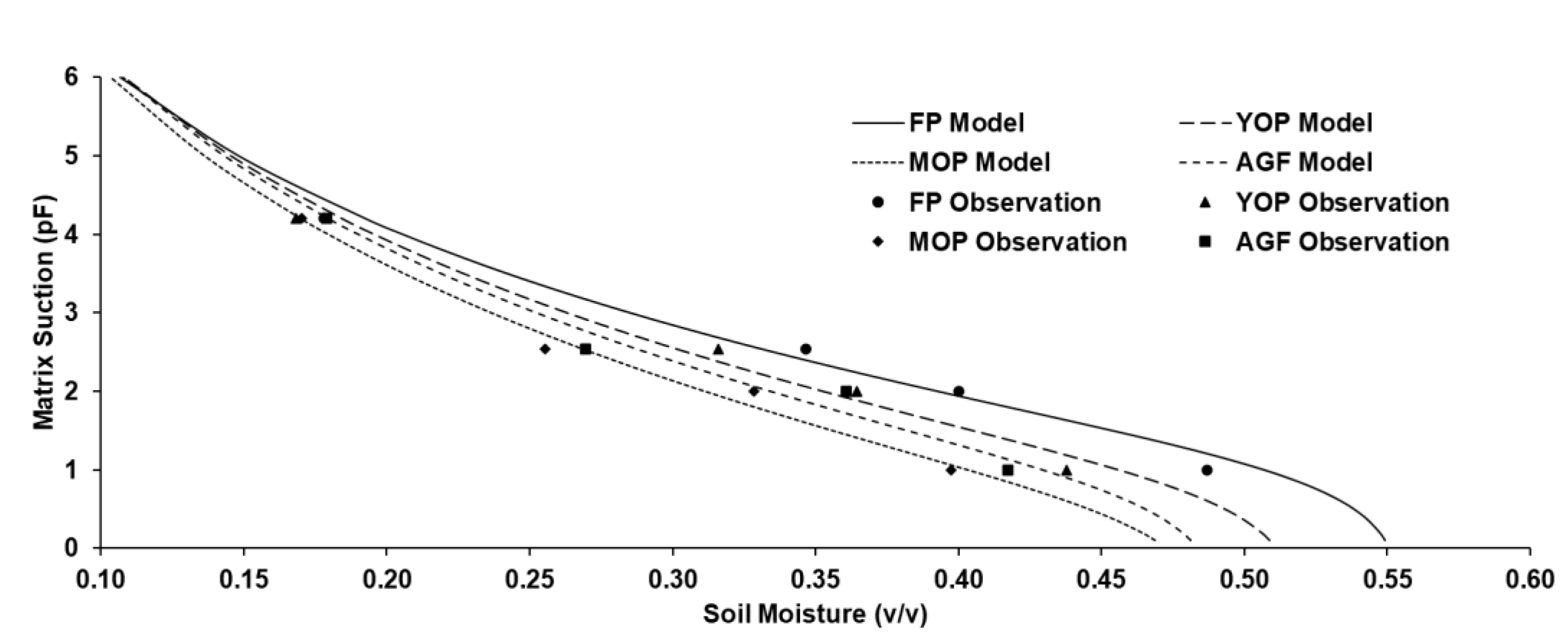
Due to soil compaction, bulk density and soil porosity changes lead to soil water retention changes. The soil water retention curve (SWRC) is presented in Figure 2, showing that the trend of soil water retention in each land use has the same pattern as the soil porosity: FP > YOP > AGF Ex-MOP > MOP. These results indicate that FP has the highest soil water retention for the same potential energy, while MOP has the lowest. The best-fit van Genuchten parameters obtained from adjustments are presented in Table 2. The SWRC of each land use has high suitability to the observed data, evidenced by a low RMSE and high R-squared. Parameter n and m are related to the slope of the retention curve after the inflection point (S) [10]. The S value is often used to describe the level of soil degradation. The results obtained indicate that MOP has the highest level of soil degradation, while FP is the lowest.
Precipitation or irrigation that infiltrates the soil column moves freely under gravitational force, and the soil matrix binds the rest by adhesive force. Gravitational water occupies drainage pores or the range of soil pores between saturated water content and field capacity (pF 0–pF 2.54). FP has higher saturated water content, field capacity, and drainage pores (Table 3), which indicates that FP has more gravitational water than YOP and MOP. Land use with high gravitational water has implications for higher percolation, lateral flow, and groundwater recharge, evidenced by SWAT simulation. Soil water bound by soil matrix is divided into available water content (AWC) or water that plant roots can still absorb and permanent wilting point (PWP) or water that plant roots can no longer absorb. AWC is the water content occupying the available water pore space (pF 2.54–pF 4.2). In contrast, PWP occupies the unavailable water pore space (pF ≥ 4.2). FP with high available water pore space implies that FP holds more soil water as a source for the plant uptake and evapotranspiration process.
3.2. Evaluation of Water Regulation Ecosystem Services
The performance of the calibrated SWAT was evaluated quantitatively based on statistical values compared to the criteria recommended by Abbaspour [27], Moriasi [29], and Ayele [30]. The model’s performance is very good for the calibration period, with NSE 0.78 and R-squared 0.88, and suitable for the validation period, with NSE 0.67 and R-squared 0.83. In addition, the p-Factor and r-Factor obtained are 0.93 and 1.09 for the calibration period and 0.75 and 0.54 for the validation period, which indicates model uncertainty is acceptable. Based on the literature review, 20 key parameters capable of capturing the main WRES were selected for calibration and 7 of them were the most sensitive parameters based on the Latin hypercube sensitivity analysis (Table 4).
All calibrated parameters are CN2 (curve number in average moisture conditions) and OV_N (manning “n” coefficient for overland flow) that related with surface runoff; LAT_TTIME (lateral flow travel time) that related with lateral flow; CH_N2 (manning “n” coefficient for the main channel), CH_K2 (hydraulic conductivity of the main channel), CH_N1 (manning “n” coefficient for tributary channel), and ALPHA_BNK (riverbank recession constant) that related with streamflow routing; CANMX (maximum canopy storage), ESCO (soil evaporation compensation coefficient), and EPCO (plant uptake compensation factor) that related evapotranspiration; ALPHA_BF (baseflow recession constant) and GWQMN (baseflow threshold) that related baseflow; and REVAPMN (water level threshold for “revap”), GW_DELAY (groundwater delay), and RCHRG_DP (deep aquifer recharge proportion) that related groundwater recharge. Furthermore, all observed parameters are SOL_BD (bulk density), SOL_Z (soil depth), SOL_AWC (available water content), and SOL_CBN (soil carbon content) that related with soil water storage; and SOL_K (soil permeability) that related with lateral flow. The initial value of curve number (CN2) and manning “n” coefficient for overland flow was based on frequently used and reliable literature.
The three parameters related to streamflow routing are sensitive parameters, such as ALPHA_BNK, CH_K2, and CH_N2. ALPHA_BNK is the most sensitive parameter, indicated by the highest |T-stat|. The sensitivity of ALPHA_BNK, CH_K2, and CH_N2 indicates that the flow routing mechanism influenced by these parameters greatly determines the streamflow dynamics. The sensitivity of CH_K2 shows that streamflow is strongly influenced by two-way interactions between rivers and shallow aquifers, where this interaction only occurs in intermittent rivers. Rivers receive water from shallow aquifers when the water table level exceeds the riverbed (rainy season) and lose water when the water table level is less than the riverbed (dry season). The velocity of streamflow filling and loss is closely related to the hydraulic conductivity of the soil layer (CH_K2) between the riverbed and the shallow aquifer. CH_N2 is also a sensitive parameter, which means that the flow velocity greatly determines the streamflow dynamics. Higher CH_N2 is associated with lower flow rates, while lower CH_N2 is associated with higher flow rates.
The other sensitive parameters are CN2, ESCO, SOL_BD, and GWQMN. As a component that dominates streamflow during the rainy period, the magnitude of surface runoff calculated from the CN2 value also dramatically determines the streamflow dynamics. Previous studies have shown that CN2 is always a sensitive parameter when the CN method is chosen for rainfall–runoff modeling [33]. CN2 has a value range of 0 to 100, but the often-used values are in the range of 25 to 98. The greater the CN2 value, the higher the surface runoff generated from rainfall. SOL_BD is a parameter that determines the soil water retention, which then implies soil moisture dynamics. Soil moisture dynamics are necessary to determine surface runoff, lateral flow, groundwater recharge, and actual evapotranspiration. The last, GWQMN, is a parameter that determines the amount of baseflow, where baseflow only appears if the water table exceeds the GWQMN value.
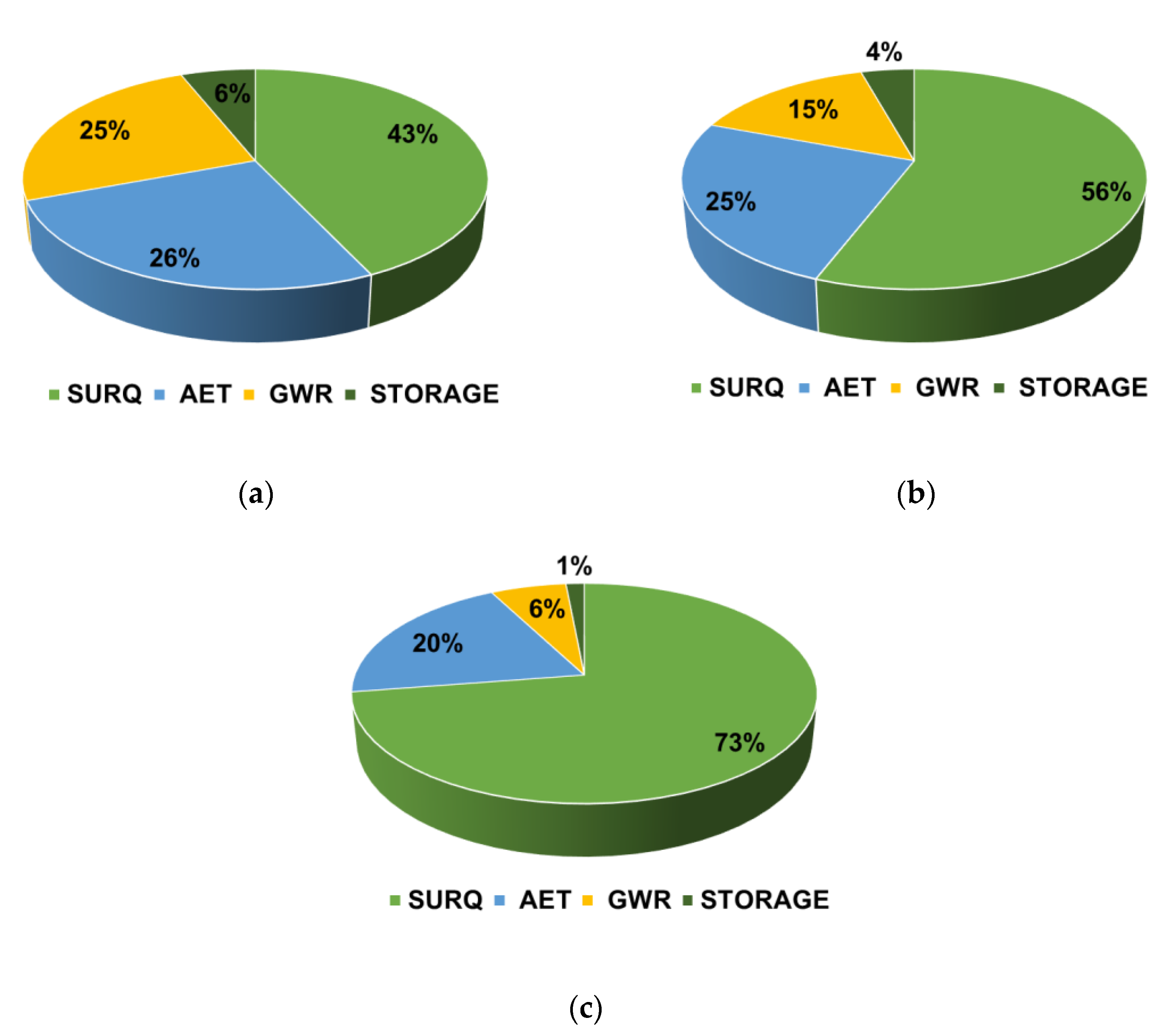
The SWAT model used for evaluating WRES has been updated by adding soil water retention characteristics in the HRU scale. The soil water retention characteristics are inputted into soil attributes and affect the WRES value for each HRU after HRU definition. Soil water retention characteristics are related to calculating curve number retention parameter and defining soil moisture ranges that affect surface runoff, evapotranspiration, and soil water storage. Precipitation that reaches soil surface is generally allocated as surface runoff (SURQ), groundwater recharge (GWR), actual evapotranspiration (AET), and soil water storage (SW) (Figure 3). In forest patches (FP), 43% of rainfall is distributed as SURQ, 26% as AET, 25% for GWR, and 6% for SW. On the other hand, on mature (MOP) and young (YOP) oil palm plantations, rainfall is allocated as SURQ by 56% and 73%, respectively, AET by 25% and 20%, and GWR 15% and 6%. The temporal WRES of each land use is presented in Figure 4. The area of agroforestry plots on former oil palm plantations (AGF ex-MOP) are very narrow (<0.01% of the watershed area) and do not significantly affect the landscape-scale water regulation. Therefore, these agroforestry plots are not included in the SWAT simulation.
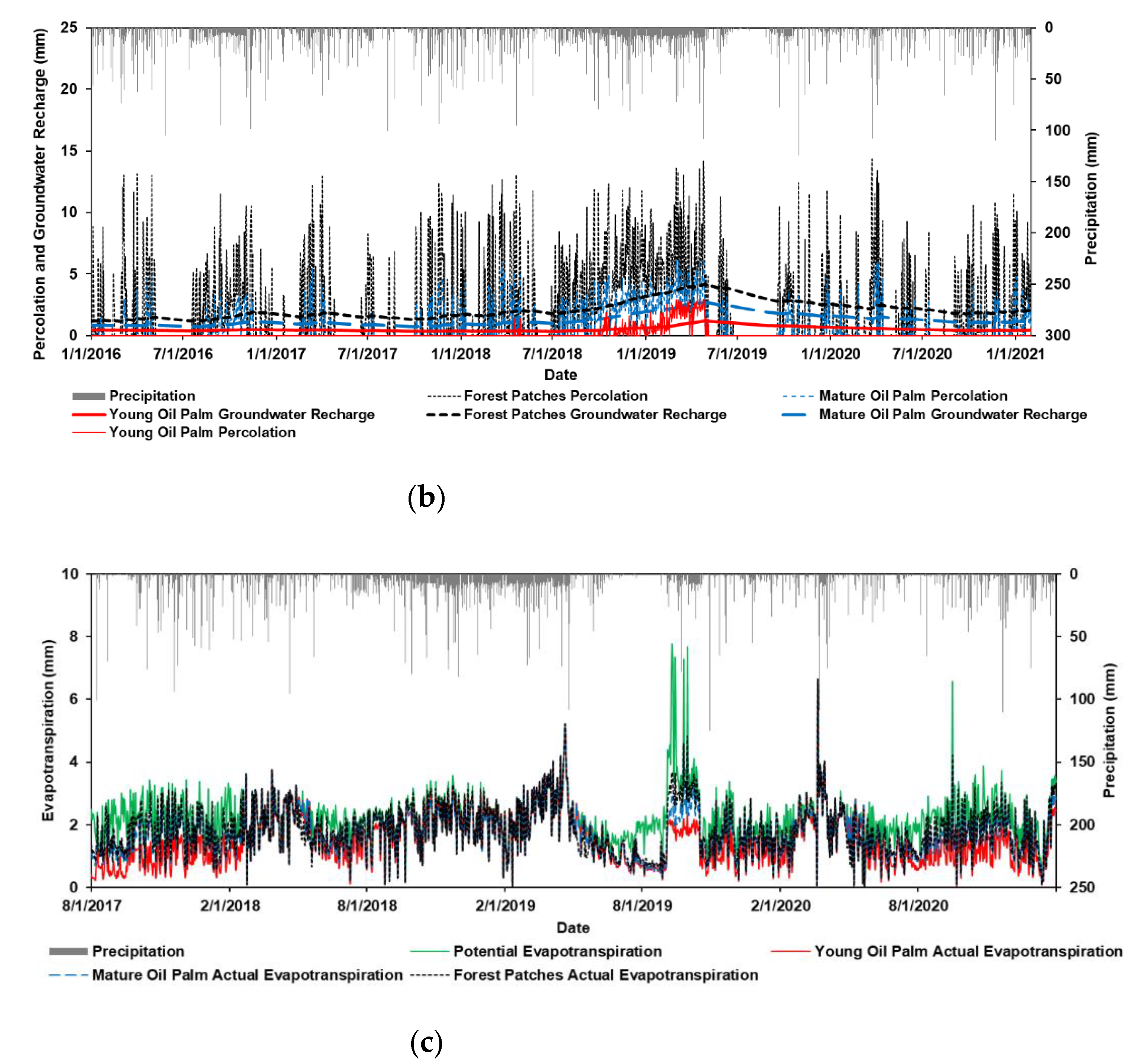
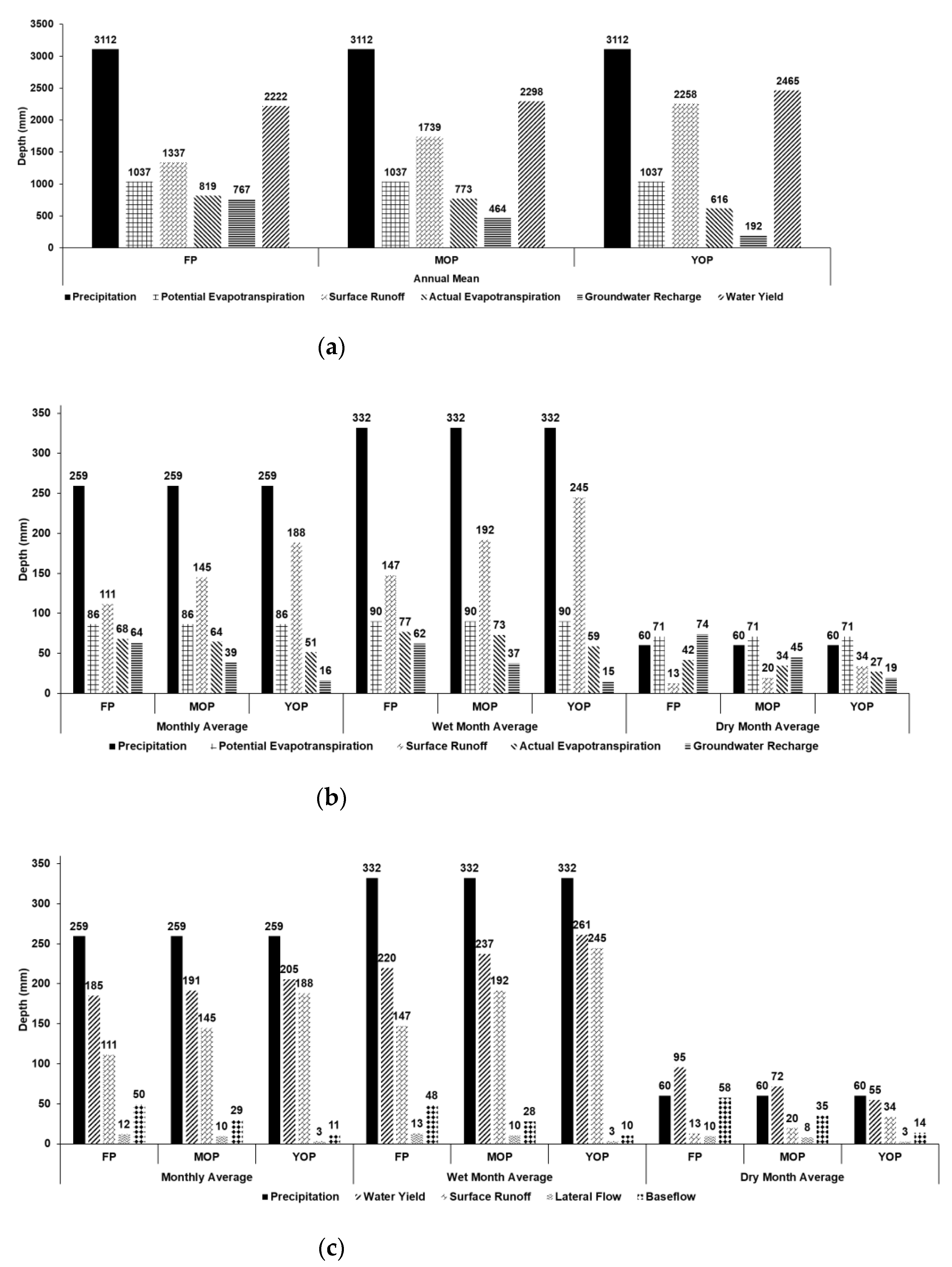
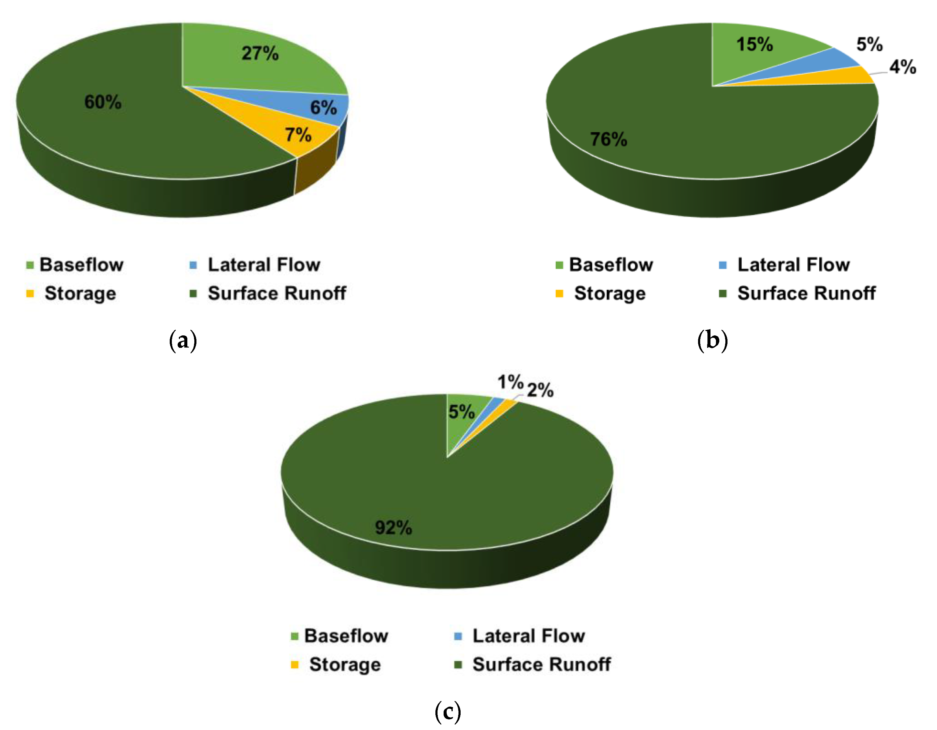
Forest patches have better annual and monthly water regulation ecosystem services than young and mature oil palm plantation, evidenced by lower surface runoff, higher groundwater recharge, higher actual evapotranspiration, higher soil water storage, lower water yield in wet months, and higher water yield in dry months (Figure 5). The annual water yield of forest patches is 2222 mm, while the average water yield in the wet and dry months is 220 mm and 95 mm. On the other hand, the annual water yield of young and mature oil palms were 2465 mm and 2298 mm, wet month water yields were 261 mm and 237 mm, and dry month water yields were 55 mm and 72 mm. The annual and seasonal water yield difference between forest patches and young oil palms is very high and decreases as the oil palm grows [2]. An increasing proportion of surface runoff and decreasing lateral flow and base flow to water yield in mature and young oil palm led to more significant water yield seasonal variability despite the higher annual water yield (Figure 6). It means that oil palm water yield became concentrated in the rainy season and decreased in the dry season, while forest patch water yield is less concentrated in the rainy season and more available in the dry season.
Actual evapotranspiration (AET) is also an essential component of water regulation ecosystem services because it plays a role in crop production (water use) and microclimate regulation. The annual actual evapotranspiration of forest patches was 819 mm, with a monthly average of 77 mm in the wet months and 42 mm in the dry months. Meanwhile, the annual actual evapotranspiration of young and mature oil palms was 773 mm and 616 mm, with an average of 73 mm and 59 mm in the wet months and 34 mm and 27 mm in the dry months. Potential evapotranspiration (PET) and soil moisture at available water content (AWC) are the main limiting factors for AET. PET limits AET in saturated soil, while AWC limits AET in unsaturated soil. FP with higher AWC implied higher AET than YOP and MOP. AET values were also controlled by canopy cover, quantified by the leaf area index (LAI) by direct measurement using hemispherical photos. FP with LAI of 3.1 ± 0.63 had a higher AET than MOP with LAI of 1.27 ± 0.19. FP has an AET/PET coefficient of 0.79, while YOP and MOP are 0.59 and 0.75. This value means that, from 100% of the potential energy allocated for the evapotranspiration, FP uses 79% of that energy to evaporate water, while YOP uses 59%, and MOP uses 75% of potential energy.
4. Discussion
Water regulation through the soil layer is the primary process determining how much water flows above the soil surface as surface runoff, returns to the atmosphere through evapotranspiration, percolates into the aquifer, and is stored in the soil pores. Water regulation is highly dependent on soil quality, which is indicated by soil physical, chemical, and biological characteristics that vary in response to soil type, land use, and topography [34]. Water regulation through the soil layer also determines the retention and movement of dissolved nutrients, such as nitrogen, phosphorus, and other nutrients. Therefore, good soil quality needs to be maintained to support sustainable agricultural production. However, a decline in soil quality has led to soil degradation mainly caused by anthropogenic pressures exerted on the soil beyond its carrying capacity [35].
Soil degradation in the form of soil compaction is a consequence that must be accepted due to natural ecosystem changes to agroecosystems, especially intensive monoculture-cultivated agriculture, such as oil palm plantation [34,36,37]. Soil compaction in the oil palm plantation is characterized by increased soil bulk density and decreased porosity. On the other hand, ecosystem restoration, such as preserving forest patches or constructing agroforestry islands inside oil palm plantations, will improve soil structure indicated by increased porosity and reduced bulk density. Soil compaction in oil palm plantations is mainly caused by soil structure detachment by heavy equipment pressure during soil tillage and harvesting, intensive inorganic fertilization, and decreased soil organic matter and vegetation cover [38].
Soil compactions have negative effects on the soil hydrological process, such as reduction in infiltration capacity, permeability, and soil water retention that are related with reduction in soil porosity [39]. This phenomenon, in turn, has implications for the WRES degradation. For example, [5,6] reported that the study area experienced increasing problems related to water resources due to soil compaction in the oil palm plantations area, especially the prolonged water shortage during the dry season. Based on soil water retention curve interpretation in MOP and YOP, the soil is degraded and less structured, has less organic matter, and has fewer pores. Meanwhile, FP has more structured soil with more organic matter and pores. According to [10], the SWRC slope (S value) correlates with soil bulk density, porosity, and soil organic matter content. The S value will decrease along with the increase in bulk density, decrease in porosity, and decrease in soil organic matter.
The higher the level of soil compaction causes the macropores to be further reduced, which causes the field capacity, saturated water content, and gravitational water to decrease. The decrease in gravitational water can be seen from the reduction in lateral flow, percolation, and groundwater recharge. On the other hand, soil compaction effect on water retention characteristics is almost nonexistent at very high matrix suction (pF > 4.2) [40,41]. Water retention at a high matrix suction tends to be influenced by textural pores associated with clay content. The higher the clay content, the higher the water retained by the textural pores [42,43]. Soil compaction only changes the structural pores and does not change the textural pores. For the same soil type, although there are differences in AWC and gravitational water associated with different land management, the water content in the high suction matrix tends to be the same [41]. The modeling result proves that each SWRC in the study area tends to coincide when the suction matrix gets bigger, considering that the soil in the study area has relatively the same clay content based on soil texture data from ground survey and laboratory analysis.
The SWAT model assisted in WRES upscaling from plot scale to landscape and time-series scale. Nevertheless, before further interpretation, it is necessary to evaluate the reliability and uncertainty of the SWAT model through the NSE, R-squared, p-Factor, and r-Factor values. The objective function used during the calibration process is NSE, meaning that the value of each parameter will be optimized from its initial value until it reaches the desired NSE value. When the system calculates the NSE value, other statistical values, such as R-squared, will be adjusted automatically. In addition, evaluation of model uncertainty is vital because SWAT provides various combinations of parameters and different modules that produce one of the same outputs but produce another very different output. A good model has a p-Factor value close to 1 and an r-Factor close to 0. However, to achieve a p-Factor close to 1, it is necessary to sacrifice the r-Factor value away from 0 and vice versa. Therefore, the best simulation is defined as a balanced p-Factor and r-Factor when it reaches the highest NSE or R-squared value during the calibration and validation periods. To obtain a balanced p-Factor and r-Factor, we must arrange each model parameter’s lower and upper bound.
The calibrated results are still in the reliable category, and the model’s uncertainty is still acceptable, although the model’s performance for the validation period is not as good as the calibration period. The high values of R2 and NSE in the calibration and validation periods indicate that the combination of calibrated parameters can capture the impact of daily meteorological input variations on daily WRES. Moriasi [29] stated that the model reliability criteria could be used for model evaluation on a monthly and daily scale. However, with the same criteria, model evaluation for the daily scale is generally more robust than the monthly one because daily output captures variations and inaccuracies arising from parameter uncertainty and daily input data (SWAT input must be daily, while the output can be daily or monthly). More accurate modeling of WRES for micro-watersheds can serve as complementary information for environmental restoration planning at a local scale. A calibrated and validated SWAT model with acceptable reliability and uncertainty was then used to evaluate WRES of forest patches among oil palm plantations.
Due to differences in soil water characteristics, WRES varies significantly between land uses and management, so changes in land use and management will impact the change in WRES at the landscape scale by routing mechanism. Meanwhile, oil palm is the dominant vegetation in the study area, so the oil palm WRES dominates the landscape-scale water balance. In addition, given the dynamic nature of oil palm plantations that are cleared and replanted every 20–30 years, it is necessary to understand oil palm WRES when they are young and mature (yielding plants). The transition from YOP to MOP occurs 8–9 years after planting, when the canopy cover reaches its maximum value. The simulation consistently shows that preserving forest patches among oil palm plantations has implications for decreasing SURQ, increasing SW, and increasing GWR. These advantages have consequences for the FP water yield, which is higher in the dry month and lower in the wet month so that water is still available in the dry season and does not overflow in the rainy season. The lower WYLD FP compared to oil palm plantations is supported by [44], which states that the response to WYLD in agroecosystems, especially oil palm plantations, tends to be higher than forest.
SURQ occurs when rainfall exceeds infiltration capacity, where lower infiltration capacity in oil palm due to soil compaction causes more rainfall to turn into SURQ. Two factors caused the higher SURQ, and more insufficient water storage in oil palm plantations: (1) decreased canopy and ground cover in YOP and (2) intensive soil compaction due to MOP harvesting. The decrease in canopy and ground cover causes the SURQ rate to be faster, time concentration to be shorter, and decreases in interception and evapotranspiration. The rough surface of the FP due to more complex canopy stratification, cover crops, and forest litter, besides lowering SURQ, also slows the SURQ rate on its way to water bodies. High infiltration capacity also increases LAT, BFO, and GWR. LAT and BFO are relatively stable WYLD parts because they have a slower rate to reach water bodies. LAT and BFO indicate the river regime’s sustainability as it maintains water availability on a day without rain. An increase in SURQ and a decrease in LAT, BFO, and GWR lead to an increased risk of flooding, drought, and water scarcity. Changes in local water resources had become a significant concern for residents in the study area, including the faster shallow aquifer depletion during the dry season and high fluctuations in streamflow between the rainy and dry season [5].
High canopy cover in FP also causes soil water storage to be more compensated for the AET besides reducing SURQ. High AET increases the initial abstraction and decreases rainfall proportion for SURQ. Three factors limit AET: PET as an energy source, AWC as a water source, and stomatal conductance (correlated with LAI) as the water pump from the soil to the atmosphere. A high AET causes soil moisture to decrease faster so that the soil water changes more quickly from saturated to unsaturated conditions. Unsaturated soils have higher infiltration rates and lower SURQ rates than saturated soils, so, in this case, AET plays a role in reducing runoff. AET is also an essential element of surface energy balance related to microclimate regulation. A higher AET for the same net radiation will reduce the proportion of energy for atmosphere heating (sensible heat). The increase in air temperature in the study area is evidence of the relationship between lower AET in oil palm plantations (especially YOP) and atmospheric warming. Beside depletion in groundwater, the residents in the study area also feel the air has become much warmer since oil palm plantations have dominated the landscape [5]. In addition, the comparison of lower PET and AET in oil palm plantations (especially in the dry season) indicates that these land uses have a higher water deficit than FP.
FP has properties like a sponge and a pump in the hydrological cycle. Meanwhile, MOP only has pump properties, and YOP does not have these two properties. FP act like sponges by increasing soil water retention and releasing it slowly through LAT and BFO because it has more soil pores. Water is stored and maintained on days without rain and even remains available until the dry season through these properties. On the other hand, FP also act like pumps by evaporating a large amount of soil water into the atmosphere. The proof that MOP only has pump properties is that MOP evaporates a large amount of water, although not as much as FP, but cannot store large amounts of soil water. YOP does not have sponge and pump properties, indicated by low AET and low soil water storage. The unavoidable soil degradation due to soil compaction is the leading cause of oil palm plantations losing their sponge properties. The loss of sponge properties due to soil compaction has three consequences: a decrease in infiltration leading to an increase in SURQ, a reduction in the GWR, and a decrease in AWC leading to a reduction in AET.
The anecdotal information that oil palm plantations are “water-greedy crops” [5,45] because they have higher AET and are associated with water scarcity is inaccurate. The MOP AET tends to be less than equal to FP [2], while YOP AET is much lower. More scientific evidence for this water scarcity case is that oil palm plantations encounter soil compaction so that more rainfall flows become SURQ than stored in soil pores. Oil palm water use is greater than the stored water because of improper management, where high AET is not accompanied by high AWC and GWR, as is the case with FP. Higher AET also reduces shallow aquifers through the capillary water movement to plant roots when soil moisture is insufficient to compensate for AET, which causes the groundwater to be dwindled and become unavailable during the dry season.
WRES sustainability is mainly determined by land use and management, which changes the soil and surface and affects rainfall distribution into SURQ, GWR, and AET [46]. According to locals’ information that there is a groundwater decline during the dry season as the primary water source, the desired alternative for water management is to reduce SURQ and increase GWR. Landscape SURQ can be reduced and GWR can be increased through a multifunctional landscape, i.e., retaining the remaining FP among oil palm plantations. By maintaining FP or agroforestry as a high conservation area with an optimal area, soil and water conservation becomes a more suitable alternative for improving landscape WRES while maintaining oil palm productivity. FP with good soil structure and more complex canopy stratification enhance the WRES, so their existence in a landscape dominated by oil palm plantations is vital to maintaining the watershed’s ecological integrity. In addition, the presence of FP inside oil palm plantations can synergize the provisioning and regulating services, where oil palm provides provision ecosystem services and FP provide regulation ecosystem services. The recommended multifunctional landscape is to maintain FP or create agroforestry islands separately around oil palm plantations. If oil palm is mixed with forest vegetation, there will be competition for light and water, which hinders the productivity of the entire vegetation.
Multifunctional landscapes also enhance other ecosystem services besides WRES, such as biodiversity conservation and erosion prevention [47]. Multifunctional landscapes are also an effort to adapt to the negative impacts of climate change. Changes in rainfall patterns due to climate change, where rainfall is predicted to increase in wet months and decrease in dry months causes WRES variations to become more extreme [48]. Further research is needed regarding the spatial configuration of multifunctional landscapes with the most optimum ecosystem functions and economic benefits based on ecosystem services trade-offs. Another aspect that needs to be considered is that the chosen multifunctional landscapes policies must be site-specific and examine the local biophysical characteristics of the landscape, such as soil type, topography, and elevation [49,50]. Even more broadly, they need to include social and economic factors. For example, soil type in the study area belongs to the hydrologic soil group (HSG) C based on the observation of soil permeability, where the runoff coefficient of each land use is higher than HSG A or HSG B. In addition, the topography in the study area belongs to the relatively flat areas, where the runoff coefficient is lower than the steeper slope. Environmental planners require these site-specific quantitative relationships to balance landscape-scale ecological and socio-economic functions.
5. Conclusions
Multifunctionality landscapes approach through maintaining forest patches between oil palm plantations, can improve landscape WRES, shown by a decrease in surface runoff, an increase in groundwater recharge, an increase in soil water storage, and an increase in actual evapotranspiration. As a result, water is not concentrated in the rainy season and remains available in the dry season. The forest patches can improve landscape WRES because they have good soil hydrological characteristics, so the existence of forest patches is essential to maintain the ecological integrity of the watershed. Soil hydrological characteristics in forest patches are indicated by the lowest bulk density and the highest soil porosity compared to oil palm plantations. Good soil hydrological characteristics have implications for increasing soil water retention, imply more soil water is stored and available to plants (available water content), and flows through soil pore spaces to fill aquifers and river networks (gravitational water). Meanwhile, soil compaction increases bulk density, decreases porosity, and decreases soil water retention in oil palm plantation.
The calibrated SWAT is reliable and acceptable model, shown by the high NSE and R-squared value and balanced p-Factor and r-Factor values. The SWAT model consistently proves that forest patches have sponge and pump properties in the hydrological cycle. The sponge properties are related to the optimal distribution of soil porosity so that water is stored in the rainy season and flows slowly during the dry season. Meanwhile, the pump properties are related to plant tissue, which plays a role in absorbing and returning soil water to the atmosphere to maintain microclimate stability. Mature oil palm can only evaporate large amounts of water like forest patches but cannot retain some soil water because of degraded soil pores due to soil compaction. The pump properties, which are not accompanied by the sponge properties, cause the water use to be greater than the stored water. Therefore, the multifunctional landscape approach by conserving forest patches between oil palm plantations is one approach that can improve the sustainability of oil palm plantations. The multifunctional landscape can synergize provisioning services from oil palm plantations and regulating services from forest patches.
Author Contributions
Y.K. and S.T. designed the research. Y.K. wrote the manuscript. S.T., T.J., E.D.W. and B.S. reviewed the manuscript. All authors have read and agreed to the published version of the manuscript.
Funding
This research was funded by PMDSU (Program Pendidikan Magister Menuju Doktor untuk Sarjana Unggul) scholarship from Ministry of Education, Culture, Research, and Technology, Republic of Indonesia.
Data Availability Statement
The datasets presented in the study are included in the article material; further inquiries can be directed to the corresponding author/s.
Acknowledgments
This research was supported by CRC-990 EFForTS (Collaborative Research Center 990 Ecological and Socio-economic Functions of Tropical Lowland Rainforest Transformation System) in form of access to the study site and provision of daily meteorological data.
Conflicts of Interest
The authors declare no conflict of interest.
References
- Ewers, R.M.; Scharlemann, J.P.W.; Balmford, A.; Green, R.E. Do increases in agricultural yield spare land for nature? Glob. Chang Biol. 2009, 15, 1716–1726. [Google Scholar] [CrossRef]
- Dislich, C.; Keyel, A.C.; Salecker, J.; Kisel, Y.; Meyer, K.M.; Auliya, M.; Barnes, A.D.; Corre, M.D.; Darras, K.; Faust, H.; et al. A review of the ecosystem functions in oil palm plantations, using forests as a reference system. Biol. Rev. 2017, 92, 1539–1569. [Google Scholar] [CrossRef] [PubMed]
- Tarigan, S.; Wiegand, K.; Sunarti; Slamet, B. Minimum forest cover required for sustainable water flow regulation of a watershed: A case study in Jambi Province, Indonesia. Hydrol. Earth Syst. Sci. 2018, 22, 581–594. [Google Scholar] [CrossRef] [Green Version]
- Sharma, S.K.; Baral, H.; Laumonier, Y.; Okarda, B.; Komarudin, H.; Purnomo, H.; Pacheco, P. Ecosystem services under future oil palm expansion scenarios in West Kalimantan, Indonesia. Ecosyst. Serv. 2019, 39, 100978. [Google Scholar] [CrossRef]
- Merten, J.; Röll, A.; Guillaume, T.; Meijide, A.; Tarigan, S.D.; Agusta, H.; Dislich, C.; Dittrich, C.; Faust, H.; Gunawan, D.; et al. Water scarcity and oil palm expansion: Social views and environmental processes. Ecol. Soc. 2016, 21, 5. [Google Scholar] [CrossRef]
- Tarigan, S.; Stiegler, C.; Wiegand, K.; Knohl, A.; Murtilaksono, K. Relative contribution of evapotranspiration and soil compaction to the fluctuation of catchment discharge: A case study from a plantation landscape. Hydrol. Sci. J. 2020, 65, 1239–1248. [Google Scholar] [CrossRef]
- Millenium Ecosystem Assessment (MEA). Ecosystem and Human Well-Being: Synthesis; Island Press: Washington, DC, USA, 2005. [Google Scholar]
- Bolliger, J.; Battig, M.; Gallati, J.; Klay, A.; Stauffacher, M.; Kienast, F. Landscape multifunctionality: A powerful concept to identify effects of environmental change. Reg. Environ. Chang. 2011, 11, 203–206. [Google Scholar] [CrossRef]
- Rallings, A.M.; Smukler, S.M.; Gergel, S.E.; Mullinix, K. Towards multifunctional land use in an agricultural landscape: A trade-off and synergy analysis in the Lower Fraser Valley, Canada. Landsc. Urban Plan. 2019, 184, 88–100. [Google Scholar] [CrossRef]
- Dexter, A.R. Soil physical quality part I: Theory, effects of soil texture, density, and organic matter, and effects on root growth. Geoderma 2004, 120, 201–214. [Google Scholar] [CrossRef]
- van Genuchten, M.T. A closed-form equation for prediction the hydraulic conductivity of unsaturated soils. Soil Sci. Soc. Am. J. 1980, 4, 892–898. [Google Scholar] [CrossRef] [Green Version]
- Wei, Z.; Zhang, B.; Liu, Y.; Xu, D. The application of a modified version of the SWAT model at the daily temporal scale and the hydrological response unit spatial scale: A case study is covering an irrigation district in the Hei River basin. Water 2018, 10, 1064. [Google Scholar] [CrossRef] [Green Version]
- Arnold, J.G.; Srinivasan, R.; Muttiah, R.S.; Williams, J.R. Large area hydrologic modeling and assessment part I: Model development. JAWRA J. Am. Water Resour. Assoc. 1998, 34, 73–89. [Google Scholar] [CrossRef]
- Neitsch, S.L.; Arnold, J.G.; Kiniry, J.R.; Williams, J.R. Soil and Water Assessment Tool Theoretical Documentation Version 2009; Texas A&M University: Commerce, TX, USA, 2011. [Google Scholar]
- Dash, S.S.; Sahoo, B.; Raghuwanshi, N.S. A novel embedded pothole module for soil and water assessment tool (SWAT) improving streamflow estimation in paddy dominated catchments. J. Hydrol. 2020, 588, 125103. [Google Scholar] [CrossRef]
- Zhang, H.; Wang, B.; Liu, D.L.; Zhang, M.; Leslie, L.M.; Yu, Q. Using an improved SWAT model to simulate hydrological responses to land use change: A case study of a catchment in tropical Australia. J. Hydrol. 2020, 585, 124822. [Google Scholar] [CrossRef]
- Sajikumar, N.; Remya, R.S. Impact of land cover and land-use change on runoff characteristics. J. Environ. Manag. 2015, 161, 460–468. [Google Scholar] [CrossRef]
- Wang, Y.; Jiang, R.; Xie, J.; Zhao, Y.; Yan, D.; Yang, S. Soil and water assessment tool (SWAT) model: A systematic review. J. Coast. Res. 2019, 93, 22–30. [Google Scholar] [CrossRef]
- Zhang, D.; Lin, Q.; Chen, X.; Chai, T. Improved curve number estimation in SWAT by reflecting the effect of rainfall intensity on runoff generation. Water 2019, 11, 163. [Google Scholar] [CrossRef] [Green Version]
- Gao, X.; Chen, X.; Biggs, T.W.; Yao, H. Separating wet and dry years to improve the calibration of SWAT in Barret Watershed, Southern California. Water 2018, 10, 274. [Google Scholar] [CrossRef] [Green Version]
- Hawkins, R.H.; Theurer, F.D.; Rezaeianzadeh, M. Understanding the basis of the curve number method for watershed models and TMDLs. J. Hydrol. Eng. 2019, 24, 06019003. [Google Scholar] [CrossRef]
- Arsyad, S. Soil and Water Conservation; IPB Press: Bogor, ID, USA, 2009. [Google Scholar]
- Kristanto, Y.; Tarigan, S.D.; June, T.; Wahjunie, E.D. Evaluation of different runoff curve number (CN) approaches on water regulation ecosystem services assessment in intermittent micro catchment dominated by oil palm plantation. Agromet 2021, 35, 73–88. [Google Scholar] [CrossRef]
- Allen, R.G.; Pereira, L.S.; Raes, D.; Smith, M. Crop evapotranspiration-guidelines for computing crop water requirements. In FAO Irigation and Drainage Paper 56; Food and Agriculture Organization: Rome, IT, USA, 1998. [Google Scholar]
- Dash, S.S.; Sahoo, B.; Raghuwanshi, N.S. How reliable are the evapotranspiration estimates by soil and water assessment tool (SWAT) and variable infiltration capacity (VIC) models for catchment-scale drought assessment and irrigation planning? J. Hydrol. 2021, 592, 125838. [Google Scholar] [CrossRef]
- Dile, Y.T.; Karlberg, L.; Srinivasan, R.; Rockstrom, J. Investigation of the curve number method for surface runoff estimation in tropical regions. JAWRA J. Am. Water Resour. Assoc. 2016, 52, 1155–1169. [Google Scholar] [CrossRef]
- Abbaspour, K.C. SWAT-CUP: SWAT Calibration and Uncertainty Programs—A User Manual; Swiss Federal Institute of Aquatic Science and Technology: Dübendorf, CH, USA, 2015. [Google Scholar]
- Muleta, M.; Nicklow, J. Sensitivity and uncertainty analysis coupled with automatic calibration for a distributed watershed model. J. Hydrol. 2005, 306, 127–145. [Google Scholar] [CrossRef] [Green Version]
- Moriasi, D.N.; Arnold, J.G.; van Liew, M.W.; Bingner, R.L.; Harmel, R.D.; Veith, T.L. Model evaluation guidelines for systematic quantification of accuracy in watershed simulation. Trans. ASABE 2007, 50, 885–900. [Google Scholar] [CrossRef]
- Ayele, G.T.; Teshale, E.Z.; Yu, B.; Rutherfurd, I.D.; Jeong, J. Streamflow and sediment yield prediction for watershed prioritization in the Upper Blue Nile River basin Ethiopia. Water 2017, 9, 782. [Google Scholar] [CrossRef] [Green Version]
- Singh, V.; Bankar, N.; Salunkhe, S.S.; Bera, A.K.; Sharma, J.R. Hydrological stream flow modeling on Tungabhadra catchment: Parameterization and uncertainty analysis using SWAT CUP. Curr. Sci. 2013, 104, 1187–1199. [Google Scholar]
- Jung, I.K.; Park, J.Y.; Park, G.A.; Lee, M.S.; Kim, S.J. A grid-based rainfall-runoff model for flood simulation including paddy fields. Paddy Water Environ. 2011, 9, 275–290. [Google Scholar] [CrossRef]
- van Griensven, A.; Meixner, T.; Grunwald, S.; Bishop, T.; Diluzio, M.; Srinivasan, R. A global sensitivity analysis tool for the parameters of multi-variable catchment models. J. Hydrol. 2005, 324, 10–23. [Google Scholar] [CrossRef]
- Nanganoa, L.T.; Okolle, J.N.; Missi, V.; Tueche, J.R.; Levai, L.D.; Njukeng, J.N. Impact of different land-use system on soil physicochemical properties and macrofauna abundance in the humid tropics of Cameroon. Appl. Environ. Soil Sci. 2019, 2019, 5701278. [Google Scholar] [CrossRef] [Green Version]
- Arthur, M.D.; Asamoah, E.F. Soil compaction under three different land use systems within the semi-deciduous agroecological zone of Ghana. Int. J. Plant Soil Sci. 2016, 13, 1–12. [Google Scholar] [CrossRef] [Green Version]
- Liu, X.; Herbert, S.J.; Hashemi, A.M.; Zhang, X.; Ding, G. Effects of agricultural management on soil organic matter and carbon transformation-a review. Plant Soil Environ. 2006, 52, 531–543. [Google Scholar] [CrossRef] [Green Version]
- Khormali, F.; Ajami, M.; Ayoubi, S.; Srinivasarao, C.; Wani, S.P. Role of deforestation and hillslope position on soil quality attributes of loess-derived soils in Golestan province, Iran. Agric. Ecosyst. Environ. 2009, 134, 178–189. [Google Scholar] [CrossRef]
- Hamza, M.A.; Anderson, W.K. Soil compaction in cropping systems: A review of the nature, causes, and possible solutions. Soil Tillage Res. 2005, 82, 121–145. [Google Scholar] [CrossRef]
- Liu, C.; Tong, F.; Yan, L.; Zhou, H.; Hao, S. Effects of porosity on soil-water retention curve: Theoretical and experimental aspects. Geofluids 2020, 2020, 6671479. [Google Scholar] [CrossRef]
- Dorner, J.; Sandoval, P.; Dec, D. The role of soil structure on the pore functionality of an ultisol. J. Soil Sci. Plant Nutr. 2010, 10, 495–508. [Google Scholar] [CrossRef] [Green Version]
- Fashi, F.H.; Gorji, M.; Shorafa, M. Estimation of soil hydraulic parameters for different land-uses. Modeling Earth Syst. Environ. 2016, 2, 170. [Google Scholar] [CrossRef] [Green Version]
- Gupta, S.C.; Sharma, P.P.; de Franchi, S.A. Compaction effects on soil structure. Adv. Agron. 1989, 42, 311–338. [Google Scholar]
- Assouline, S. Modeling the relationship between soil bulk density and the water retention curve. Vadose Zone J. 2006, 5, 554–563. [Google Scholar] [CrossRef]
- Goeking, S.A.; Tarboton, D.G. Forest and water yield: A synthesis of disturbance effects on streamflow and snowpack in western coniferous forests. J. For. 2020, 118, 172–192. [Google Scholar] [CrossRef] [Green Version]
- Manoli, G.; Meijide, A.; Huth, N.; Knohl, A.; Kosugi, Y.; Burlando, P.; Ghazoul, J.; Fatichi, S. Ecohydrological changes after tropical forest conversion to oil palm. Environ. Res. Lett. 2018, 13, 064035. [Google Scholar] [CrossRef]
- Ouyang, L.; Liu, S.; Ye, J.; Liu, Z.; Sheng, F.; Wang, R.; Lu, Z. Quantitative assessment of surface runoff and base flow response to multiple factors in Pengchongjian small watershed. Forest 2018, 9, 533. [Google Scholar] [CrossRef] [Green Version]
- Tarigan, S.; Buchori, D.; Siregar, I.Z.; Azhar, A.; Ullyta, A.; Tjoa, A.; Edy, N. Agroforestry inside oil palm plantation for enhancing biodiversity-based ecosystem functions. In Proceedings of the International e-Conference on Sustainable Agriculture and Farming System, Bogor, Indonesia, 24–25 September 2020; Volume 694, p. 012058. [Google Scholar]
- Tarigan, S.; Kristanto, Y. Assessment of water security in Indonesia considering future trends in land use change and climate change. In Water Security in Asia; Babel, M., Haarstrick, A., Ribbe, L., Shinde, V.R., Dichtl, N., Eds.; Springer: Cham, Switzerland, 2021. [Google Scholar]
- Tarigan, S.; Wiegand, K.; Dislich, C.; Slamet, B.; Heinonen, J.; Meyer, K. Mitigation options for improving the ecosystem function of water flow regulation in a watershed with rapid expansion of oil palm plantation. Sustain. Water Qual. Ecol. 2016, 8, 4–13. [Google Scholar] [CrossRef]
- Tarigan, S.; Zamani, N.P.; Buchori, D.; Kinseng, R.; Suharnoto, Y.; Siregar, I.Z. Peatlands are more beneficial if conserved and restored than drained for monoculture crops. Front. Environ. Sci. 2021, 9, 749279. [Google Scholar] [CrossRef]
Figure 1.
Study area.

Figure 2.
Soil water retention curve for each land use.

Figure 3.
Distribution of water regulation ecosystem service elements in forest patches (a), mature oil palm (b), and young oil palm (c). Notes: SURQ: surface runoff, AET: actual evapotranspiration, GWR: groundwater recharge, STORAGE: soil water storage.
Figure 3.
Distribution of water regulation ecosystem service elements in forest patches (a), mature oil palm (b), and young oil palm (c). Notes: SURQ: surface runoff, AET: actual evapotranspiration, GWR: groundwater recharge, STORAGE: soil water storage.

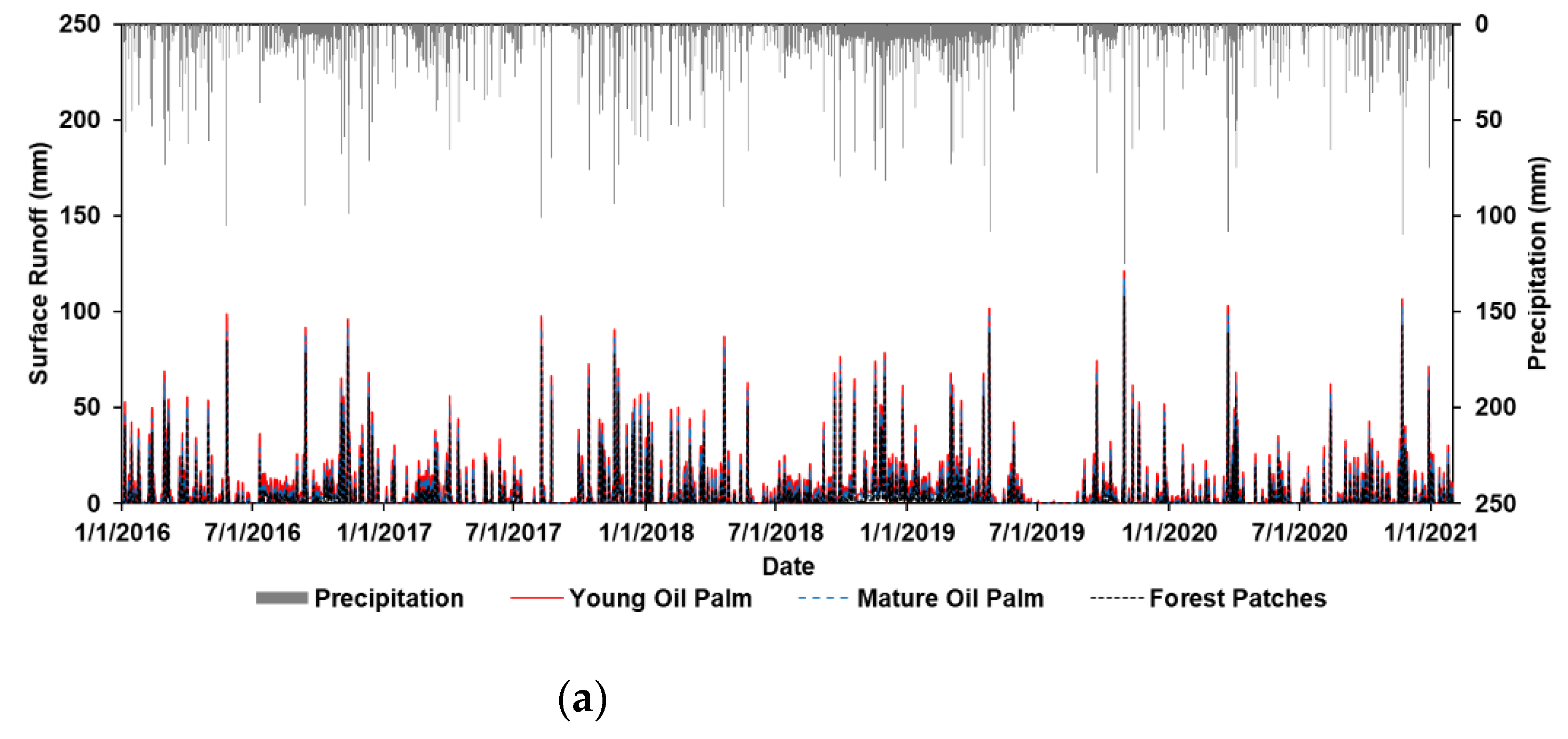
Figure 4.
Hydrograph of water regulation ecosystem service elements: surface runoff (a), groundwater recharge (b), actual evapotranspiration (c).
Figure 4.
Hydrograph of water regulation ecosystem service elements: surface runoff (a), groundwater recharge (b), actual evapotranspiration (c).


Figure 5.
Annual (a) and seasonal mean of water regulation ecosystem services (b) and water yield (c) elements.
Figure 5.
Annual (a) and seasonal mean of water regulation ecosystem services (b) and water yield (c) elements.

Figure 6.
Distribution of water yield elements in forest patches (a), mature oil palm (b), and young oil palm (c).
Figure 6.
Distribution of water yield elements in forest patches (a), mature oil palm (b), and young oil palm (c).


Table 1.
The mean values of soil porosity and bulk density.
| Land Use | Porosity (%v/v) | Bulk Density * (g/cm3) | Soil Organic Matter (%) | ||||
|---|---|---|---|---|---|---|---|
| Total Pore Space * | Dainage Pores | Water Holding Pores | |||||
| pF 1 * | pF 2 * | pF 2.54 * | pF 4.2 n | ||||
| FP | 55.6 ± 1.2 a | 48.7 ± 3.4 a | 40.0 ± 3.1 a | 34.7 ± 3.6 a | 17.8 ± 4.9 | 0.91 ± 0.06 a | 5.45 ± 0.82 a |
| YOP | 52.0 ± 3.1 a,b | 43.8 ± 6.6 b | 36.5 ± 4.6 a,b | 31.6 ± 4.8 a | 16.8 ± 4.2 | 1.12 ± 0.12 b | 4.15 ± 2.39 a,b |
| MOP | 49.0 ± 5.9 b | 39.7 ± 3.9 b | 32.8 ± 3.2 b | 25.5 ± 2.2 b | 17.0 ± 2.8 | 1.35 ± 0.16 c | 2.49 ± 0.15 b |
| AGF Ex-MOP | 49.3 ± 3.6 b | 41.7 ± 3.6 b | 36.1 ± 3.0 b | 26.9 ± 2.7 b | 17.9 ± 2.2 | 1.34 ± 0.09 c | 5.19 ± 0.04 a |
* Significant at 95% level, n: not significant at 95% level; a,b,c the mean value followed by the same letter does not differ according to the DMRT.
Table 2.
SWRC best-fit parameters and S value.
| Land Use | θs (v/v) | θr (v/v) | α (pF) | n | m | S (pF−1) | R-Squared | RMSE (v/v) |
|---|---|---|---|---|---|---|---|---|
| FP | 0.556 | 0.000 | 0.110 | 1.142 | 0.124 | 0.0533 | 0.983 | 0.0151 |
| YOP | 0.520 | 0.000 | 0.200 | 1.129 | 0.114 | 0.0463 | 0.976 | 0.0153 |
| MOP | 0.490 | 0.000 | 0.437 | 1.120 | 0.107 | 0.0413 | 0.983 | 0.0112 |
| AGF | 0.493 | 0.000 | 0.230 | 1.123 | 0.110 | 0.0425 | 0.964 | 0.0172 |
Table 3.
Soil water retention characteristic on the same potential for each land use.
| Porosity (v/v) | FP | YOP | MOP | AGF Ex-MOP |
|---|---|---|---|---|
| Solid layer | 0.45 | 0.49 | 0.53 | 0.52 |
| Total pore space | 0.55 | 0.51 | 0.47 | 0.48 |
| pF 1 | 0.51 | 0.46 | 0.40 | 0.43 |
| pF 2 | 0.39 | 0.35 | 0.31 | 0.33 |
| Field capacity | 0.33 | 0.30 | 0.27 | 0.29 |
| Permanent wilting point | 0.19 | 0.18 | 0.17 | 0.18 |
| Residual pores | 0.00 | 0.00 | 0.00 | 0.00 |
| Drainage pores | 0.22 | 0.21 | 0.20 | 0.20 |
| Fast drainage pores | 0.16 | 0.16 | 0.16 | 0.15 |
| Low drainage pores | 0.06 | 0.05 | 0.04 | 0.05 |
| Water holding pores | 0.33 | 0.30 | 0.27 | 0.29 |
| Available water pores | 0.14 | 0.12 | 0.10 | 0.11 |
| Unavailable water pores | 0.19 | 0.18 | 0.17 | 0.18 |
Table 4.
SWAT calibrated parameters with their range and best-fit values.
| Parameters a | Range | Value | Sensitivity b | ||||
|---|---|---|---|---|---|---|---|
| Lower Bound | Upper Bound | Calibrated Value | Initial Value | Unit | T-Stat | p-Value | |
| v_ESCO * | 0 | 1 | 0.739 | - | 3.721 | 0.000 | |
| v_EPCO | 0 | 1 | 0.875 | - | −0.739 | 0.460 | |
| v_CANMX | 0 | 10 | 8.67 | mm | −0.479 | 0.632 | |
| r_CN2 * | −0.25 | 0.25 | 1.190 | [22] | - | 16.053 | 0.000 |
| r_OV_N | −0.2 | 0.2 | 0.842 | [32] | - | −0.138 | 0.890 |
| r_SOL_Z | −0.9 | 0.9 | 1.38 | Obs. | mm | −0.014 | 0.988 |
| r_SOL_K | −0.2 | 0.2 | 0.948 | Obs. | mm/h | 0.129 | 0.897 |
| r_SOL_AWC | −0.2 | 0.2 | 0.932 | Obs. | % | −0.650 | 0.516 |
| r_SOL_CBN | −0.2 | 0.2 | 1.159 | Obs. | % | −0.123 | 0.902 |
| r_SOL_BD * | −0.2 | 0.2 | 1.139 | Obs. | g/cm3 | −2.500 | 0.012 |
| v_LAT_TTIME | 0 | 180 | 63.54 | day | −0.178 | 0.854 | |
| v_ALPHA_BF | 0 | 1 | 0.347 | 1/h | 0.230 | 0.818 | |
| v_GWQMN * | 0 | 5000 | 3615 | mm | −2.108 | 0.035 | |
| v_REVAPMN | 0 | 500 | 296.5 | Mm | 0.435 | 0.664 | |
| v_GW_DELAY | 0 | 300 | 294.9 | day | −1.932 | 0.054 | |
| v_RCHRG_DP | 0 | 1 | 0.197 | - | −1.888 | 0.060 | |
| v_CH_N1 | 0 | 0.3 | 0.274 | - | −1.493 | 0.136 | |
| v_CH_N2 * | 0 | 0.3 | 0.122 | - | −2.192 | 0.029 | |
| v_ALPHA_BNK * | 0 | 1 | 0.187 | day | 22.880 | 0.000 | |
| v_CH_K2 * | 0 | 500 | 31.5 | mm/h | −19.43 | 0.000 | |
a v: replace the initial value with the best fit value, r: multiply the initial value with the best fit value; b parameter is sensitive when p-value < 0.05 or |T-stat| > Tα. df, sensitive parameters is marked with (*).
Publisher’s Note: MDPI stays neutral with regard to jurisdictional claims in published maps and institutional affiliations. |
© 2022 by the authors. Licensee MDPI, Basel, Switzerland. This article is an open access article distributed under the terms and conditions of the Creative Commons Attribution (CC BY) license (https://creativecommons.org/licenses/by/4.0/).
Share and Cite
MDPI and ACS Style
Kristanto, Y.; Tarigan, S.; June, T.; Wahjunie, E.D.; Sulistyantara, B. Water Regulation Ecosystem Services of Multifunctional Landscape Dominated by Monoculture Plantations. Land 2022, 11, 818. https://doi.org/10.3390/land11060818
AMA Style
Kristanto Y, Tarigan S, June T, Wahjunie ED, Sulistyantara B. Water Regulation Ecosystem Services of Multifunctional Landscape Dominated by Monoculture Plantations. Land. 2022; 11(6):818. https://doi.org/10.3390/land11060818
Chicago/Turabian StyleKristanto, Yudha, Suria Tarigan, Tania June, Enni Dwi Wahjunie, and Bambang Sulistyantara. 2022. "Water Regulation Ecosystem Services of Multifunctional Landscape Dominated by Monoculture Plantations" Land 11, no. 6: 818. https://doi.org/10.3390/land11060818
Note that from the first issue of 2016, this journal uses article numbers instead of page numbers. See further details here.