Sea Waves Transport of Inertial Micro-Plastics: Mathematical Model and Applications

Abstract

Plastic pollution in seas and oceans has recently been recognized as one of the most impacting threats for the environment, and the increasing number of scientific studies proves that this is an issue of primary concern. Being able to predict plastic paths and concentrations within the sea is therefore fundamental to properly face this challenge. In the present work, we evaluated the effects of sea waves on inertial micro-plastics dynamics. We hypothesized a stationary input number of particles in a given control volume below the sea surface, solving their trajectories and distributions under a second-order regular wave. We developed an exhaustive group of datasets, spanning the most plausible values for particles densities and diameters and wave characteristics, with a specific focus on the Mediterranean Sea. Results show how the particles inertia significantly affects the total transport of such debris by waves.

1. Introduction

In the last decades the production and consumption of plastic products has drastically increased. Most of our daily activities and behaviors involve the use of plastic, e.g., when packaging food and goods or wearing synthetic clothes, as a couple of instances among many others. It is estimated that we globally use in excess of 260 million tonnes of plastic per year, accounting for approximately 8 per cent of world oil production [1]. The proper disposal of plastic waste has consequently become a central issue of our times, still far from being completely overcome [2]. The lack of regulations and practices able to allow a sustainable and efficient waste management has often led to undesirable releases of plastic within the marine environment [3], resulting in a substantial volume of debris added to the ocean over the past 60 years [4,5,6]. Efficient policies should be aimed at reducing plastic consumption and using biodegradable materials when reliable alternatives are available, and the most recent EU directives are indeed developing in this framework.

At first sight, to face the maritime plastic pollution requires anyway a holistic comprehension of the plastic particles dynamic in seas and oceans. The need to tackle the plastic pollution threat with the utmost urgency is consequently reflecting in the attention given by the scientific community, as proved by the increasing amount of papers on such topic (a partial summary can be found in Hidalgo-Ruz et al. [7]). So far the transport of plastic particles was numerically simulated mainly assuming that, in a Lagrangian sense, the single particle is non-inertial, or, in other words, it has the same mass-density of the carrier fluid in this case the sea water [8]. Then, the fate of a single or a cluster of neutrally buoyant particles is obtained by simply solving the trajectory equation, where the particle position depends at any time on the Eulerian velocity field obtained by hydrodynamic models and/or observational data (see as an instance [9,10]). Several dynamical effects can be taken into account by a specific choice of the Eulerian velocity field, which can be though in fact as a sum of different contributions, e.g., oceanic currents, Stokes drift, Ekman drift, and a turbulent velocity component (cfr. [11,12,13,14,15,16,17,18] among others). Assuming a perfect match between sea water and plastic debris density inhibits any physical mechanism of sedimentation, which is indeed neglected when assuming neutrally buoyant particles. On the contrary, other approaches allowed to consider a settling velocity disregarding any drag-induced effect, both in a lagrangian [14,19] and in an eulerian [20] approach; the settling velocity of the particles was also taken into account in Liubartseva et al. [17], who simulated the sedimentation of particles through a statistical approach based on Montecarlo simulations. Nevertheless, it has to be pointed out that the drag may be reasonably neglected only for some regimes of the controlling parameters, i.e., Froude and Stokes number.

However, it is well known from several field measurements that micro plastic particles can attain different values of density, usually ranging from 0.85 g cm${}^{-3}$ to 1.41 g cm${}^{-3}$ for polypropylene or PP and polytetrafluoroethylene or PVC respectively, see [16,20], and the differential density of the plastic debris can play an important role in the transport dynamics, especially for dimensions proper of the micro-plastic class. Furthermore, in sea waters the density of plastic particles can be dramatically modified due to biological effects, so that even particle lighter than sea water may start to settle and rise with specific periods [21,22]. In view of the above, we used a model that allows to compute the trajectory of micro-plastic particles by taking into account both the buoyancy of the particle and the drag of the flow. We referred to micro-plastics, e.g., particles characterized by diameters smaller than 5 mm, according to the definition of Arthur et al. [23]. These pieces of debris are of particular concern as they are difficult to intercept and, moreover, they are easily ingested by most of the marine species [24,25].

The paper is structured as follows: in Section 2 the numerical model employed and the testing sets are introduced. Then, in Section 3 results are shown and further discussed and summarized in Section 4.

2. Methods

The model proposed allows to assess time-dependent plastic accumulation along the z vertical direction in the 2D x-z plain, under second-order regular linear waves, referring to a prescribed particle volumetric concentration. To this end, we reproduced a sequence of particle releases representing an infinite availability of micro-plastics at a given location, under different initial conditions. We varied the parameters that might affect the settling and/or the suspension of the particles, as their physical properties (size and density distribution) as well as the sea state features (wave heights and periods). The numerical experiments provided quantitative information regarding the path followed by plastic particles owing to the Stokes drift, their horizontal (x component) and vertical (z component) velocities and, finally, on their vertical distribution.

This section formulates the conceptual model adopted in this study. It shows the wave and the particle dynamics equations, which are solved numerically in order to obtain the trajectories of the inertial particles representing the plastic debris.

2.1. Wave Model and Plastic Particle Transport Model

The flow is described by a second order monochromatic Stokes wave. The velocity field is defined on a vertical plane $(x,z)$; the vertical and horizontal Eulerian velocities (w and u respectively) are therefore expressed as:

$$\begin{array}{c}\hfill w(x,z,t)=\left(\frac{gka}{\omega }\right)f_{d1}sin(kx-\omega t)+\left(\frac{g{\left(ka\right)}^2}{\omega }\right)f_{d2}sin2(kx-\omega t)\end{array}$$

(1)

$$\begin{array}{c}\hfill u(x,z,t)=\left(\frac{gka}{\omega }\right)f_{c1}cos(kx-\omega t)+\left(\frac{g{\left(ka\right)}^2}{\omega }\right)f_{c2}cos2(kx-\omega t),\end{array}$$

(2)

where x and z are the horizontal and the vertical coordinates of the 2D plane, a is the wave amplitude, k is the wave number and $\omega$ is the angular frequency. The functions $f_{c1}$, $f_{c2}$, $f_{d1}$ e $f_{d2}$ are hyperbolic functions of the water depth h and the vertical coordinate z and read:

$$\begin{array}{ccc}\hfill f_{c1}& =& cosh\left(ks\right)/cosh\left(kz\right);\hfill \\ \hfill f_{c2}& =& 3cosh\left(2ks\right)/4{sinh}^3\left(kz\right)cosh\left(kh\right);\hfill \\ \hfill f_{d1}& =& sinh\left(ks\right)/sinh\left(kz\right);\hfill \\ \hfill f_{d2}& =& 3sinh\left(2ks\right)/4{sinh}^3\left(kz\right)cosh\left(kh\right),\hfill \end{array}$$

having defined s as $(h+z)$.

The dispersion relation linking k and $\omega$ can be expressed as follow:

$$\omega =k{U}_0+\sigma$$

(3)

where $U_0$ is the value of a possible background uniform current velocity and $\sigma$ is the frequency of the wave in the moving frame of reference [26].

Following this approach, the motion of a small inertial particle is described by the following set of equations [27]:

$$\begin{array}{ccc}\hfill \frac{d\mathbf{x}\left(t\right)}{dt}& =& \mathbf{V}\left(t\right)\hfill \end{array}$$

(4)

$$\begin{array}{ccc}\hfill \frac{d\mathbf{V}\left(t\right)}{dt}& =& \frac{\mathbf{u}(\mathbf{x},t)-\mathbf{V}\left(t\right)}{\tau }+(1-\beta )\mathbf{g}+\beta \frac{d\mathbf{u}(\mathbf{x},t)}{dt}\hfill \end{array}$$

(5)

where $\mathbf{V}\left(t\right)$ is the Lagrangian particle velocity at the position $\mathbf{x}\left(t\right)$. This set of equations describes the trajectories of small inertial particles as response to a flow field $\mathbf{u}(\mathbf{x},t)$ and subjected to a Stokes drag and gravity $\mathbf{g}$. The latter effect is taken into account through the added-mass effect represented by the dimensionless parameter $\beta$, while drag response is taken into account in the first term of the second member of Equation (5) through the Stokes response time $\tau$:

$$\begin{array}{ccc}\hfill \beta & =& {\displaystyle \frac{3{\rho }_f}{{\rho }_f+2{\rho }_p}}\hfill \end{array}$$

(6)

$$\begin{array}{ccc}\hfill \tau & =& {\displaystyle \frac{d_P^2}{12\beta \nu }}\hfill \end{array}$$

(7)

where ${\rho }_f$ and ${\rho }_p$ are the fluid density and particle density respectively, $d_P$ is the particle diameter and $\nu$ is the kinematic viscosity of the fluid. Note that the well known Stokes number can be readily evaluated as $S_t=\omega \tau$. As a matter of fact, the Stokes number is generally defined as the ratio between the characteristic times of particles ($\tau$) and flow. In this case, the characteristic time of the flow is set equal to ${\omega }^{-1}$, precisely. For $S_t<<1$ the particle can be regarded as a passive drifter and tends to behave as a fluid particle, whereas for Stokes number of order 1 ($O\left(S_t\right)\simeq 1$), inertial effects dominate leading to a behaviour dissimilar from that of passive tracers. It is worth to point out that, in the unlikely case that the plastic particle density matches the density of the fluid, Equations (4) and (5) naturally lead to the trajectory equations used to simulate a passive tracer.

The present study resumes and extends the work of Santamaria et al. [28], where the model of Maxey & Riley [27] was solved for a first order monochromatic wave. Similarly, DiBenedetto et al. [29] referred to the same wave model and weakly inertial particles (i.e., $S_t<<1$), investigating how the shape of the latter might affect their resulting trajectories. In this work, we consider a second order monochromatic wave rather than a first order one, thus the Stokes drift directly arises from the wave model with no need to superimpose additional effects. Moreover, we include a possible uniform current ($U_0$) and we do not pose any limitation on $S_t$ nor we rely on the deep water assumption for resolving the wave length $\lambda$. Finally, it is worth to mention that the model here introduces only applies to spherical particles. Although the shape of a particle is known to affect its settling velocity, this effect was shown to be not of primary importance [30]. Indeed, this geometrical simplification is often adopted in the studies of the fate of particle debris based on the trajectory equation (see [14,15,20] among others), thus the results of the present analysis will refer to it.

2.2. Description of the Numerical Experiments

The set of differential Equations (4) and (5) was numerically solved employing a Runge-Kutta method of the fourth order with adaptive steps. The Eulerian wave velocity field ($\mathbf{u}(\mathbf{x},t)$), which appears in Equation (5), was analytically solved from the relationships of Equations (1) and (2). By inspecting the model equation it appears clear that several parameters shall be defined to characterize a single experiment. Sea waves were defined through their amplitude (a) and period (T), while the other parameters were derived accordingly to the dispersion relation (see Equation (3)). Plastic particles were instead characterized through their densities and diameters. We modeled plastic particles with a diameter ranging from 100 $\mathsf{\mu }$m to 2 mm and with relative densities ranging from 0.95 to 1.25. Note that most of the numerical simulations were performed with “heavy” particles, i.e., for ${\rho }_p/{\rho }_f>1$.

Table 1. List of parameters used for the numerical experiments.

Exp.	a (m)	T (s)	$\mathit{H}/\left({\mathit{g}\mathit{T}}^2\right)$	${\mathit{U}}_0$ (m/s)	h (m)	${\mathit{d}}_{\mathit{p}}$ ($\mathsf{\mu }$m)	${\mathit{\rho }}_{\mathit{p}}/{\mathit{\rho }}_{\mathit{f}}$	$\mathit{\beta }$	$\mathit{\tau }$ (s)	# of Runs
1	1	4	0.013	0	300	100–2000	1.05–1.25	0.86–0.97	0.001–0.34	40
2	0.5	4	0.006	0	300	100–2000	1.05–1.25	0.86–0.97	0.001–0.34	40
3	0.75	4	0.01	0	300	100–2000	0.95	1.03	0.0008–0.32	20
4	0.75	4	0.01	0	300	100–2000	1.05–1.25	0.86–0.97	0.001–0.34	40
5	1.25	4	0.016	0	300	100–2000	1.05–1.25	0.86–0.97	0.001–0.34	40
6	0.32	8	0.001	0	300	100–2000	1.05–1.25	0.86–0.97	0.001–0.34	40
7	0.63	8	0.002	0	300	100–2000	1.05–1.25	0.86–0.97	0.001–0.34	40
8	0.95	8	0.003	0	300	100–2000	1.05–1.25	0.86–0.97	0.001–0.34	40
9	1.26	8	0.004	0	300	100–2000	1.05–1.25	0.86–0.97	0.001–0.34	40
10	1.57	8	0.005	0	300	100–2000	1.05–1.25	0.86–0.97	0.001–0.34	40
11	2.2	8	0.007	0	300	100–2000	1.05–1.25	0.86–0.97	0.001–0.34	40
12	0.17	6	0.001	0	300	100–2000	1.05–1.25	0.86–0.97	0.001–0.34	40
13	0.35	6	0.002	0	300	100–2000	1.05–1.25	0.86–0.97	0.001–0.34	40
14	0.53	6	0.003	0	300	100–2000	1.05–1.25	0.86–0.97	0.001–0.34	40
15	0.71	6	0.004	0	300	100–2000	1.05–1.25	0.86–0.97	0.001–0.34	40
16	0.88	6	0.005	0	300	100–2000	1.05–1.25	0.86–0.97	0.001–0.34	40
17	1.23	6	0.007	0	300	100–2000	1.05–1.25	0.86–0.97	0.001–0.34	40
18	0.26	6	0.001	0	300	100–2000	1.05	0.97	0.0009–0.34	20
19	0.53	6	0.003	0	300	100–2000	1.05	0.97	0.0009–0.34	20
20	0.8	6	0.005	0	300	100–2000	1.05	0.97	0.0009–0.34	20
21	1.05	6	0.006	0	300	100–2000	1.05	0.97	0.0009–0.34	20
22	1.32	6	0.007	0	300	100–2000	1.05	0.97	0.0009–0.34	20
23	1.59	6	0.009	0	300	100–2000	1.05	0.97	0.0009–0.34	20
24	1.59	6	0.009	0.2	300	200–2000	1.05	0.97	0.0034–0.34	10
25	1.59	6	0.009	0	20	200–2000	1.05	0.97	0.0034–0.34	10
rand1	0.5	4	0.006	0	300	100–500	0.95–1.15	0.91–1.03	0.0009–0.02	1
rand2	0.75	4	0.01	0	300	100–500	0.95–1.15	0.91–1.03	0.0009–0.02	1
rand3	1	4	0.013	0	300	100–500	0.95–1.15	0.91–1.03	0.0009–0.02	1
rand4	1.25	4	0.016	0	300	100–500	0.95–1.15	0.91–1.03	0.0009–0.02	1

reports the parameters employed for the set of numerical experiments performed. For each numerical simulation, we fixed one parameter at a time varying the other over its relative range. The design of several series of experiments (corresponding to as many test waves) allowed us to investigate the role of inertia when the particles are transported by a Stoke wave drift and, possibly, by a uniform current. Each numerical simulation represents a conceptual model where plastic particles are readily available in a thin layer at the free surface for the entire time of the simulation. To this end, for each set we released a certain number of plastic particles every wave period and we monitored their trajectories until they reached their maximum horizontal distance. Moreover, at fixed intervals of time during the simulation, we computed the vertical distribution of the number of particles. The influence of a simultaneous presence of particles with different sizes and densities was analyzed performing dedicated simulations, named in Table 1 with the label “rand”. In these cases, a cluster with diameter and density randomly distributed was released. Finally, the influence of a bulk uniform circulation $U_0$ and of a finite sea depth was investigated with specific simulations (see runs 24 and 25 of Table 1).

2.3. Climatology of the Sea State and Selection of Wave Parameters for the Numerical Experiments

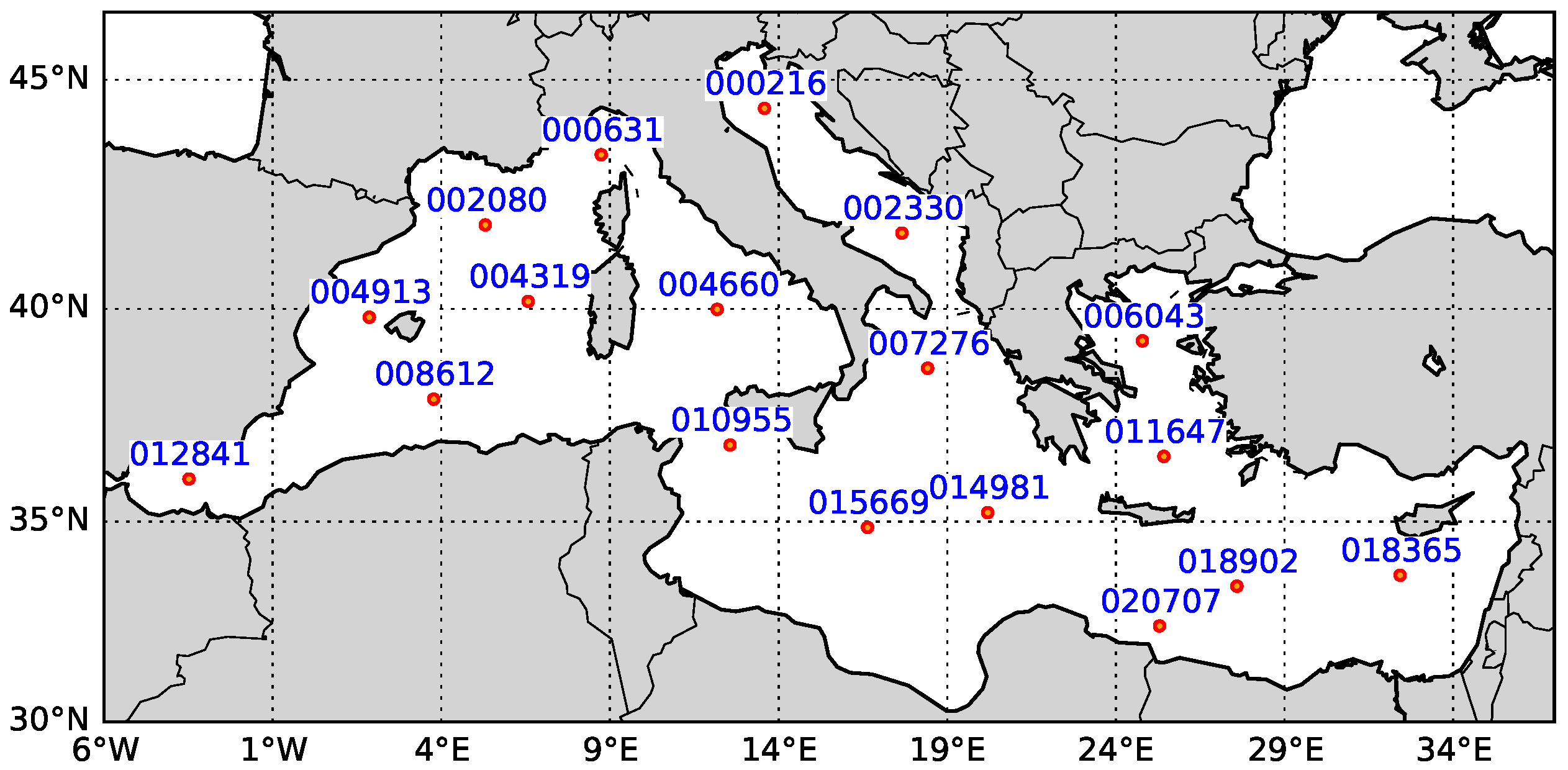
The numerical experiments require a selection of sea state parameters (a and T) to be fed into Equations (1) and (2). Then, the dispersion relationship (3) leads to the wave number. In order to employ wave parameters physically meaningful, we took advantage of a long term hindcast developed at the Authors’ department (www.dicca.unige.it/meteocean, see [31,32,33]); the dataset covers a wide time frame of 40 years (from 1979 to 2018), and is defined all over the Mediterranean sea with a lon/lat resolution of approximately 0.1°, providing the main wave features on a hourly base. For the present purpose, we analyzed time series of wave amplitude and period in several locations in the Mediterranean Sea, distributed among different basins. These locations are reported in Figure 1.

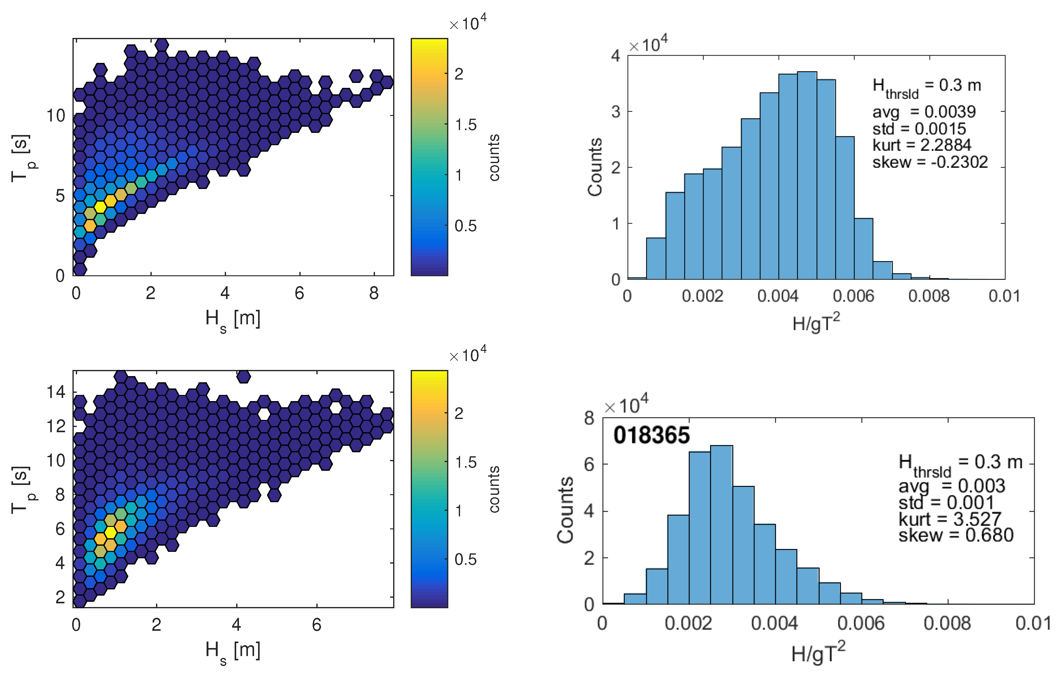
Figure 2 shows an example of the computed statistics for a couple of the selected points. We show a frequency plot of wave period against wave height H (on the left panels, having defined $H=2a$), while the histogram plots represent the frequency of occurrence (counts) of the value of the dimensionless parameter $H/g{T}^2$, having set a threshold for the wave height equal to 0.3 m in order to get rid of the not significant sea states. The parameter $H/g{T}^2$ is commonly used to synthetically describe a sea state, since it allows to define the best performing wave model according to the local bottom depth [34]. In this case, the second order Stokes wave model suited well to the environmental condition set, thus the results of the present analysis will refer to it.

$H/g{T}^2$ can be also viewed as a measure of wave steepness: for fixed values of T, increasing numbers of $H/g{T}^2$ imply higher waves; conversely, for fixed wave heights, increasing numbers of $H/g{T}^2$ imply waves with shorter periods (thus shorter wavelengths). As a general trend, locations belonging to the Mediterranean sea show similar features, due to the enclosed shape of the basin. This is subsequently reflecting on the frequency distributions of the parameter $H/g{T}^2$, which attains similar values regardless the location taken into account. As Figure 2 shows, there may exist slight differences summarized by the values of the parameters kurtosis and skewness. In fact, Point 000631 exhibits a left-skewed frequency distribution due to the higher periods characterizing the waves of the area (most likely due to the considerable length of its fetch).

On the basis of the above analysis, the wave parameters of the model were fixed in order to model reliable sea states all over the Mediterranean Sea. By looking at the values of a and T of Table 1 it can be noticed how the boundary values of $H/g{T}^2$ happen to be 0.001 and 0.016, with the upper value being slightly higher than the maximum registered among the test locations. However, most of the numerical simulations are concentrated in a narrower range, with maximum values found in the 0.002–0.04 interval.

3. Results

The following section presents the results related to different experimental designs. For all the simulations, the particles were released at x = 0.

3.1. Prediction of the Maximum Particle Horizontal Displacement

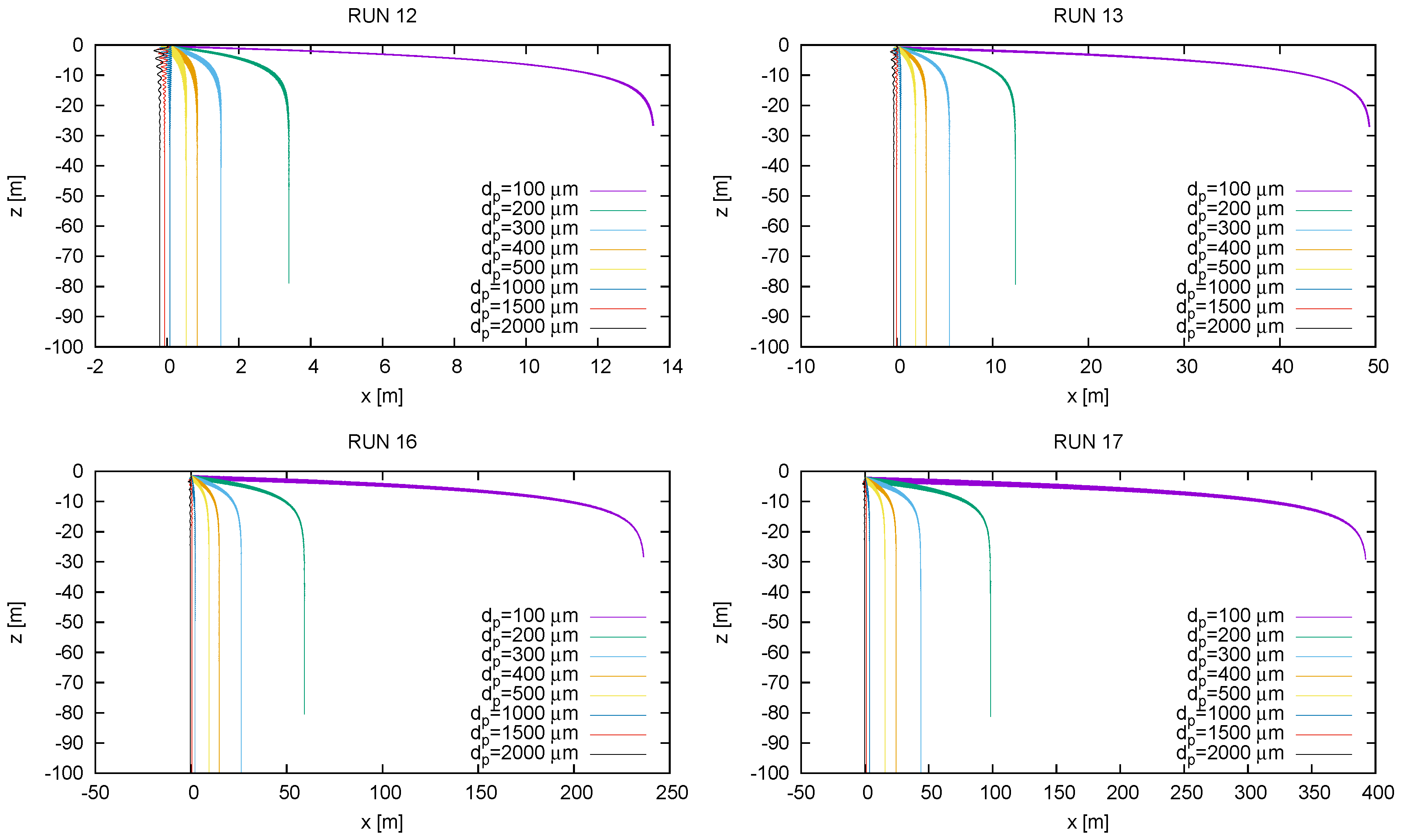
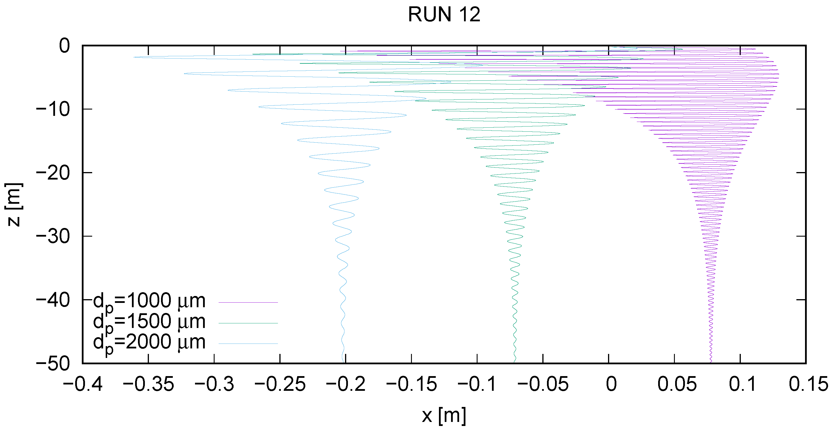
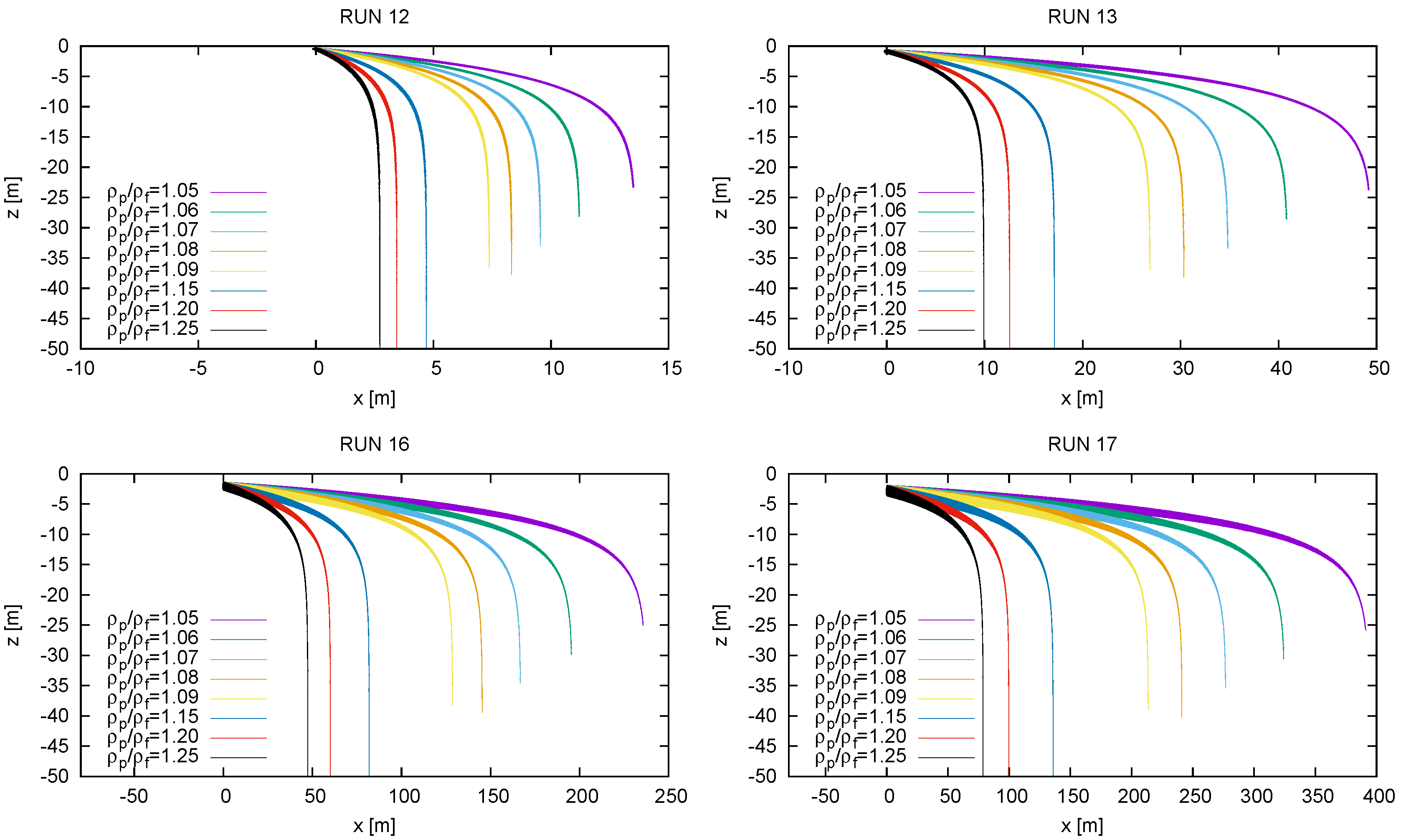
Examples of numerical trajectories on the vertical plane are shown in Figure 3. In particular, waves results are shown for values of $H/g{T}^2$ ranging from 0.001 (RUN12) to 0.007 (RUN17). The density ratio is higher than unity (${\rho }_p/{\rho }_f=1.05$), thus representative of slightly negative buoyant plastic particles. For the sake of clarity, Figure 3 shows only trajectories of few particle diameters for each run. By looking at the resulting trajectories, it appears clear that the particle diameter strongly affects the overall path. In fact, the ability of the wave induced drift to transport the particles rapidly decreases according to their increasing size: bigger debris are not able to move in the direction of wave propagation owing to the inertial effects; actually, the interplay with the Eulerian velocities and the Lagrangian particle velocities is non trivial and leads to complex trajectories, especially for larger particle sizes, that ultimately develop on the vertical direction without producing a net horizontal displacement. On the other hand, a dependence on the wave parameter $H/g{T}^2$ is still remarkable especially for small diameters of the order of hundreds of microns. Examples of the trajectories followed by particles with ${\rho }_p/{\rho }_f=1.05$ and $d_p$ = 1000, 1500, 2000 $\mathsf{\mu }$m are shown in Figure 4, which is a close up of the trajectories shown in the RUN12 panel of Figure 3. Here, it can be better appreciated how the larger particles keep the same horizontal position in which they were released.

Then, we analyzed the role of the added-mass term in the trajectory equations, summarized in the parameter $\beta$. To this end, we selected the smallest diameter analyzed in this study, e.g., $d_p$ = 100 $\mathsf{\mu }$m, varying the density ratio between 1.05 and 1.25. Results are shown in Figure 5. The resulting trajectories are qualitatively similar to those of the previous set; however, even for the heaviest particles the wave drift is able to produce a horizontal transport. It is evident that the effect of the added mass parameter $\beta$ plays a minor role with respect to the particle size, e.g., the stokes time $\tau$. At this stage, it has to be stressed that $\tau$ embeds $\beta$ as well, but depends quadratically on $d_p$.

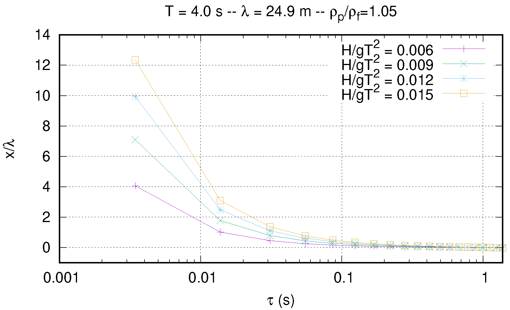
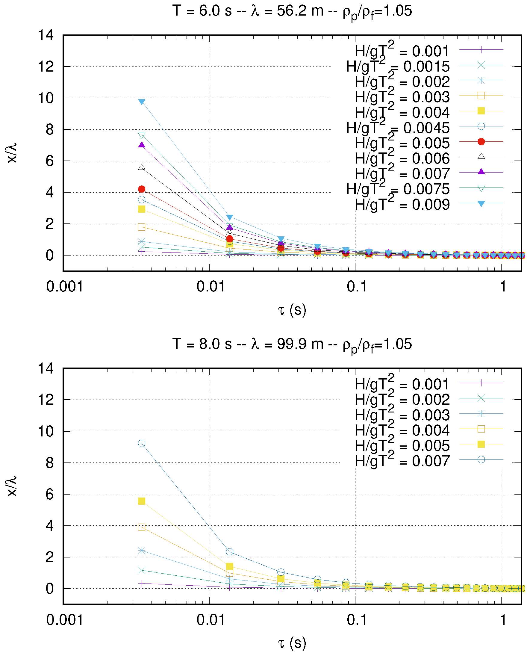
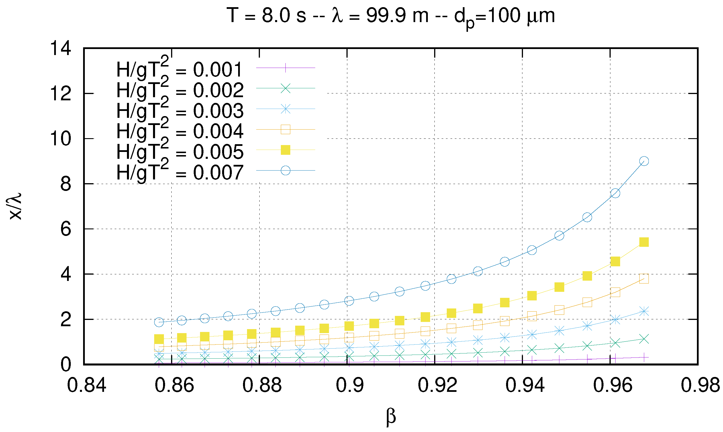
It is interesting to understand how the maximum horizontal displacement of a plastic particle depends on their properties (density and size) and on the wave characteristics. Therefore, from the total trajectories we computed the maximum horizontal distance at which a particle is no longer affected by the wave transport and continues to sink. In Figure 6 the dimensionless maximum horizontal distance ($x/\lambda$) is plotted against the Stokes time $\tau$ for different waves. Each panel corresponds to series of runs with particles with fixed density ratio and wave period T, and varying particle diameter and wave parameter $H/\left(g{T}^2\right)$. The panels are ordered from top to bottom for increasing wave periods from 4 s to 8 s. Note that the corresponding wavelength are ordered consistently owing to the dispersion relation (3), with values ranging from 24.9 m to 99.9 m. By inspecting Figure 6 it is evident that the maximum horizontal displacement strongly depends on $\tau$. Indeed, $x/\lambda$ tends to decreases rapidly as $\tau$ increases regardless the value of $H/\left(g{T}^2\right)$. However, results suggest that only sea states with significant values of $H/\left(g{T}^2\right)$ are able to transport plastic particle for a distance of the order of ten wavelength. Moreover, particles with $\tau$ greater than 0.08 are almost no longer able to be transported horizontally, i.e., $x/\lambda$ tends to be negligible. In the representation of Figure 6 results shows a residual dependence on the wave period, and this is precisely the reason for us to consider separately the maximum horizontal distances obtained.

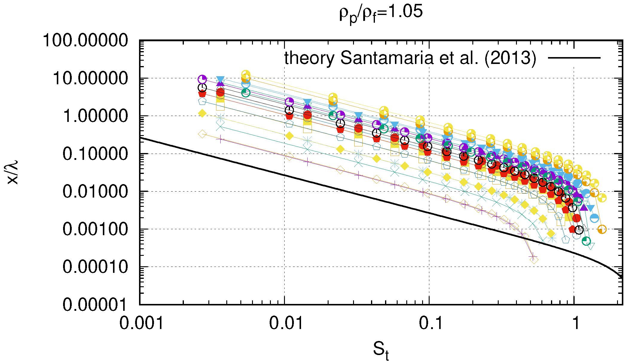
At a second time, following [28], we plotted the results due to the dimensionless Stokes number $S_t$. In this way, the values of $x/\lambda$ appear nicely ordered with increasing values of the wave parameter $H/\left(g{T}^2\right)$, as Figure 7 shows. In the same figure it is also highlighted the theoretical prediction derived perturbatively by Santamaria et al. [28], which reads:

$$x/\lambda =F_r^2\frac{1-\beta (1-\beta )S_t^2}{(1-\beta )S_t}$$

(8)

where $F_r$ is the Froude number, defined as $F_r=\omega a/c$ (c is the wave celerity). As expected, results are especially consistent for small $S_t$, as the relationship of Equation (8) was derived in the perturbative regime of small Stokes.

Finally, the maximum horizontal distance was calculated for fixed particle size ($d_p$ = 100 $\mathsf{\mu }$m) and varying densities, i.e., changing the added mass parameter $\beta$. The results are shown in Figure 8 for a given value of the wave peak period T. Again, results suggest that $\beta$ is not as much relevant as $\tau$ for the final path of a particle, in fact $x/\lambda$ decreases according to both the parameters, but at a lower rate when evaluated against $\beta$, indeed.

3.2. Influence of Stokes Drift and Inertia on the Settling Velocities of the Particles

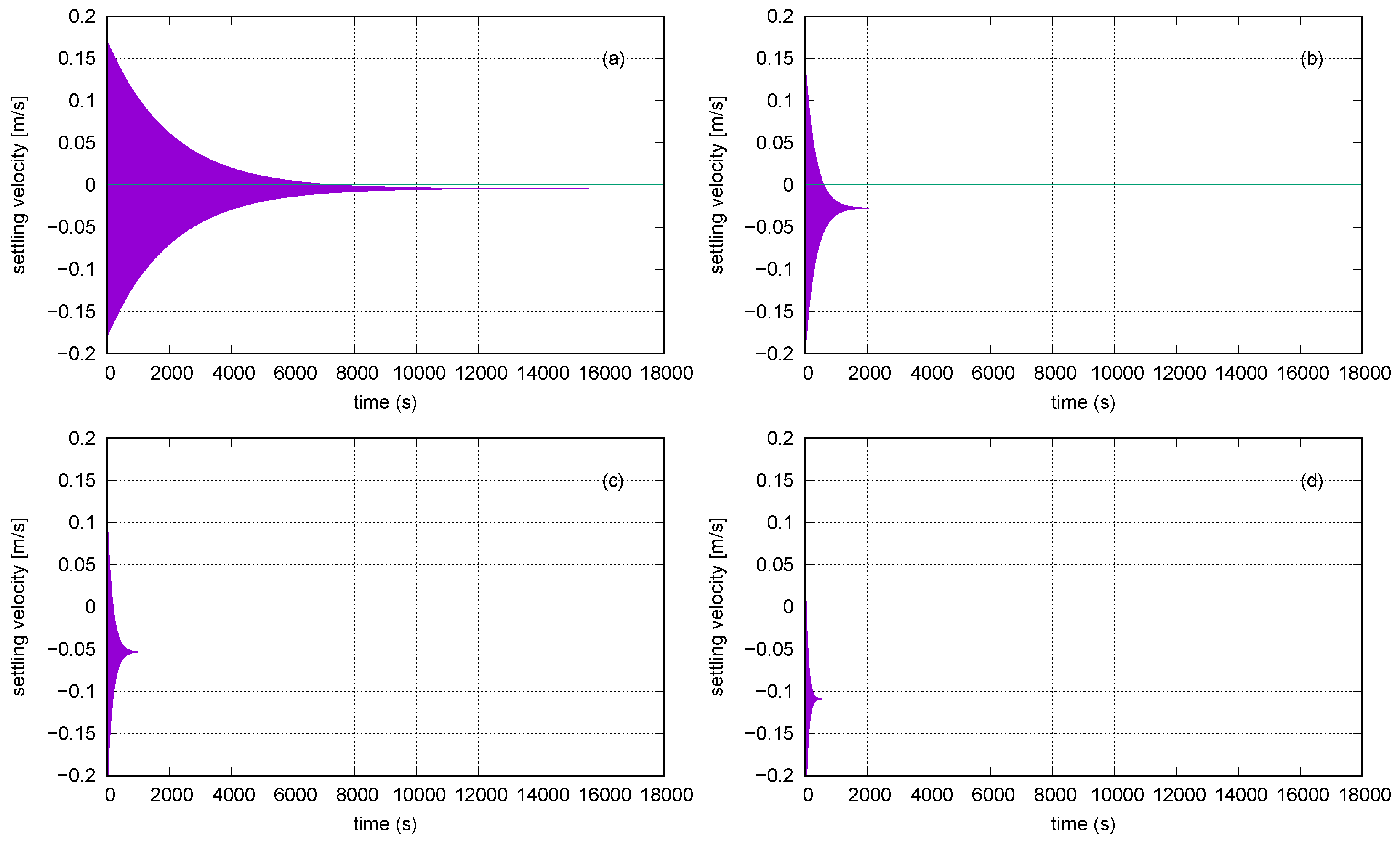
Several studies have been dedicated to the estimate of the settling velocities of plastics particles [30,35,36]. Indeed, the problem of a falling object is even a broader topic that has relevant applications in many other fields, e.g., sediment transport and in particular for suspended load. However, most of the studies concern the case of a falling particle in still fluid. The first analysis of the response of heavy particles under a sea wave is due to Santamaria et al. [28], which is extended by this study as explained in Section 2. Examples of the typical time evolution of the vertical velocity of the single inertial particle are shown in Figure 9 for different particle size $d_p$, given the density ratio and the sea state parameter.

As expected, the interaction between particles and Stokes drift leads to an evolution of the settling velocity periodic in time, which oscillates with a period equal to the period of the wave and an amplitude that tends to decrease in time, reaching a constant value for large times. Actually, the particle follows the trajectories shown in Figure 3 and Figure 5, and at every wave period heavy particles are found at larger depths, where the effect of waves is reduced. It is worth noting how, for the same wave, the response of particle of different sizes is strongly influenced by the size itself. Small particles tends to reach a constant value of settling velocity after thousands of wave periods (panel (a) of Figure 9), whereas for larger diameters such condition takes place much faster (panel (b), (c) and (d)). The asymptotic settling velocity of the particle can be written as:

$$w_s=-(1-\beta )g\tau$$

(9)

which is the well-known Stokes settling velocity. Note that $w_s$ is negative, due to the negative buoyancy of the particles.

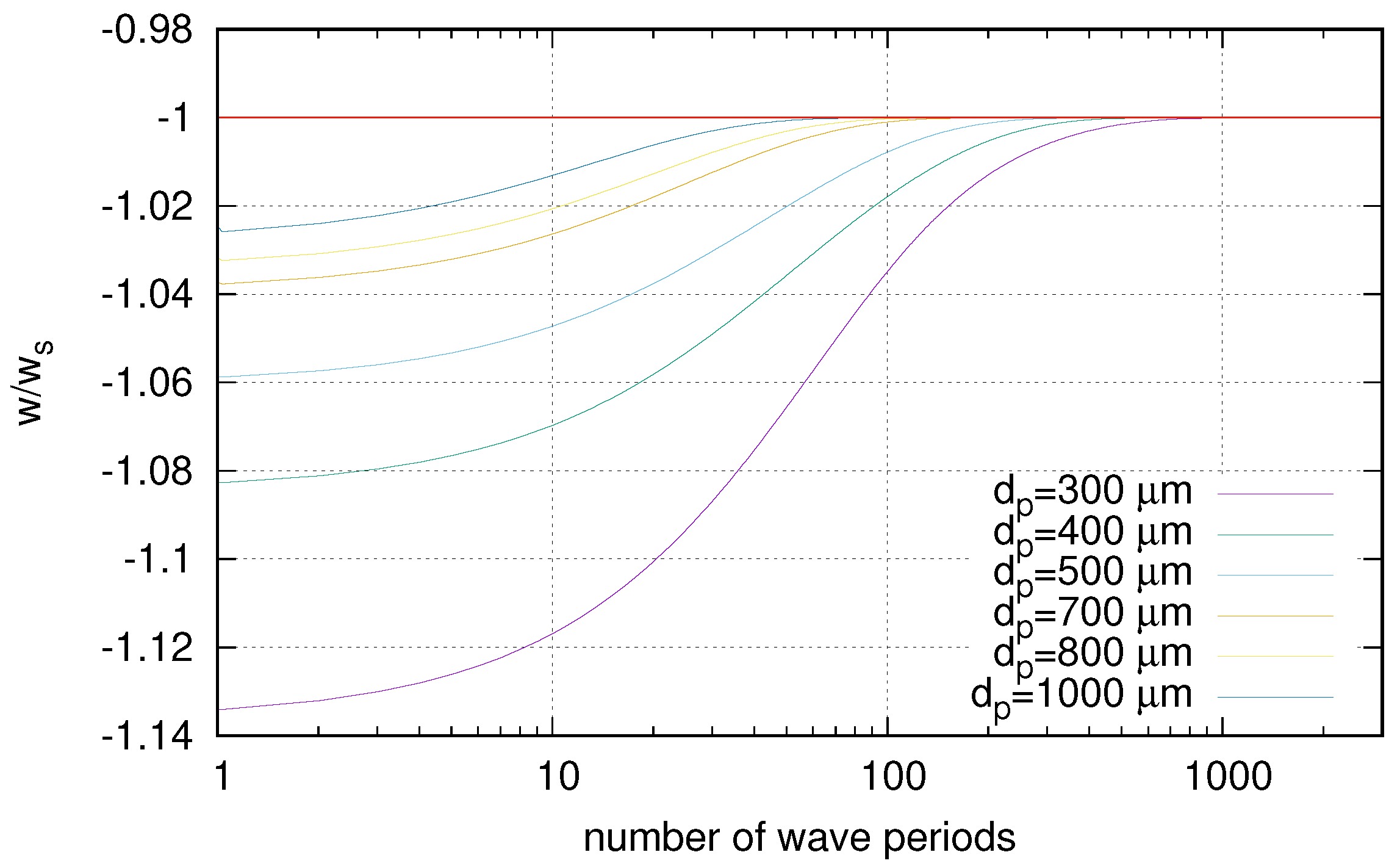
It is now interesting to deepen the evolution in time of the vertical velocity due to the changing characteristics of the particles. Figure 10 reports the time evolution of the normalized vertical velocity $\overline{w}/w_s$ for different particle sizes, given the wave parameter $H/g{T}^2$. Note that we changed the sign of the Stokes settling velocity $w_s$, so that a value of −1 corresponds to $\overline{w}=w_s$, whereas values lower than $-1$ indicate that the particle is settling with a velocity greater than the Stokes velocity. Results suggest that the behavior of $\overline{w}/w_s$ strongly depends on the particle size, i.e., for smaller particles it takes longer to sink with a velocity equals to $w_s$ (the same consideration holds for different sea waves). A similar behavior was observed by Santamaria et al. [28], thus it is clear that the interaction of the Stokes drift with the inertial character of the plastic particle yields transient regimes, where the periodic averaged vertical velocity may substantially differ with respect to $w_s$. It has to be pointed out that, in order to obtain a correct prediction of the time evolution of the particle velocity, it is crucial to select an integration time step smaller than the Stokes time $\tau$ (typically a tenth of the Stokes response time).

3.3. Vertical Distribution of Plastic Particles

The simulations developed in the present context allowed also to determine the micro-plastics distribution along the water column, and to evaluate how this depends on the particle characteristics and sea wave state. For the sake of clarity, we recall that our numerical experiments were designed continuously releasing a prescribed number of particles every wave period, right below the sea surface. The number of particles was computed after each wave period for 0.5 m wide bins, from the sea surface to the sea bottom. Then, we computed the relative frequency as the ratio of the bin count over the total number of particles released at the time of the computation and over the whole computational domain (i.e., the count of the particles only depends on the z coordinate).

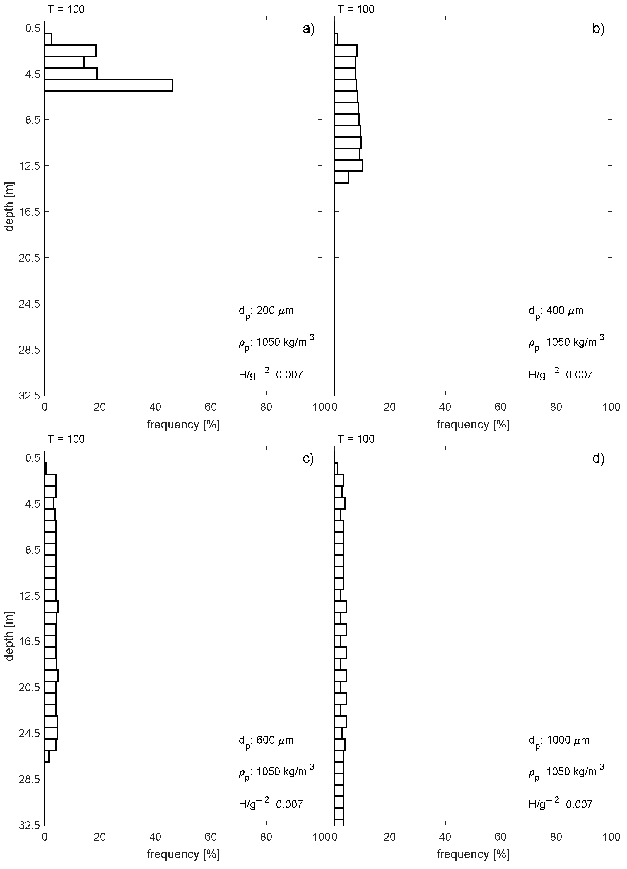
Figure 11 shows the frequency distributions for different particle sizes, given $H/g{T}^2=0.007$ and ${\rho }_p/{\rho }_f=1.05$ after 100 wave periods. The four panels help to understand the role of the particle diameter. The resulting distributions show similar profiles for diameters greater than 400 $\mathsf{\mu }$m (panel (b), (c) and (d) of Figure 11), where the negative buoyancy of the particles dominates and leads to an almost uniform profile along the water column. Only the smallest particles show a different distribution with the depth after hundreds of wave periods. This is consistent with the results discussed in Section 3.1 where the trajectories of heavy particles (diameters in the order of hundreds of microns) were shown to rapidly settle, whereas the smallest particle were drifted for longer distance along the direction of the wave propagation.

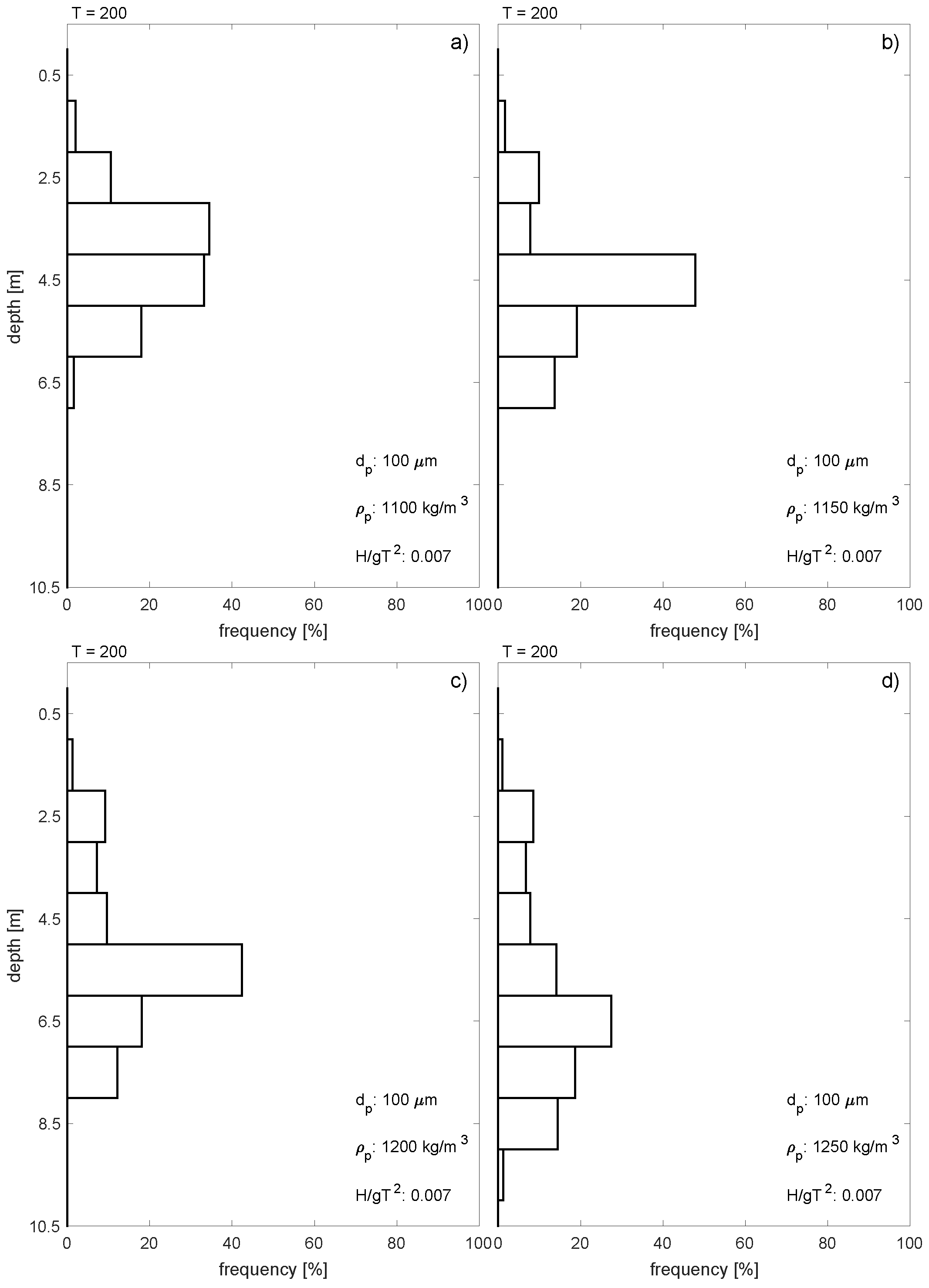
The role played by the density ratio was investigated with another series of numerical experiments, in which the particle size was kept equal to the smallest diameter $d_p$ = 100 $\mathsf{\mu }$m, whereas the particle density was changed in a range between 1050 to 1250 kg/m${}^3$. Figure 12 shows the results for $H/g{T}^2=0.007$. In particular, each panel corresponds to particles with increasing density (from (a) to (d)) after an integration time equal to 200 periods. The vertical distributions show profiles close to Gaussian in all the cases, with peaks shifted at higher depths for heavier particles. As already discussed, the added-mass parameter $\beta$ plays a minor role for the buoyancy of the particles, even for the heaviest ones (cfr. panel (d)).

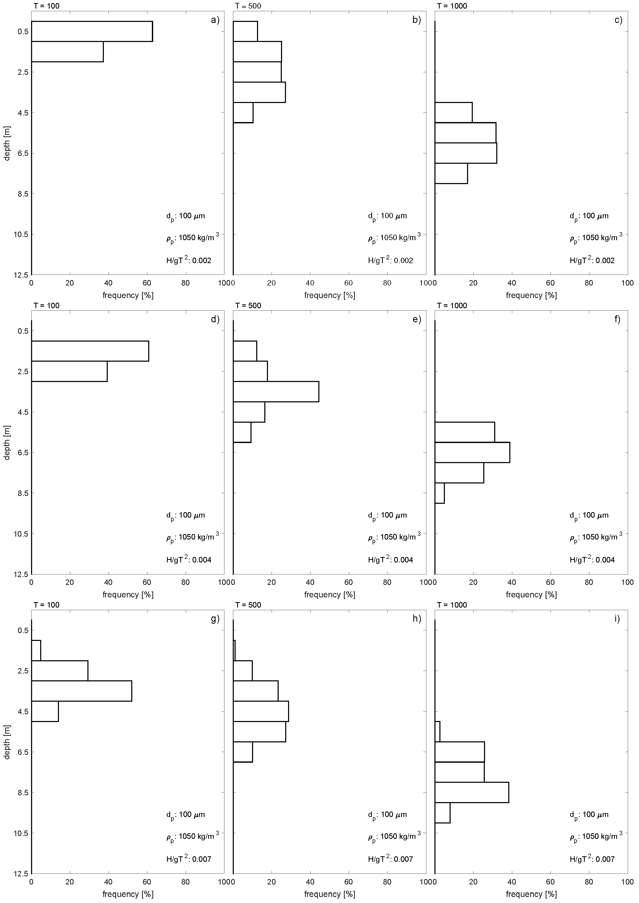
Then, Figure 13 shows the results depending on varying wave parameters. In particular, the columns corresponds to three integration time, i.e., 100, 500 and 1000 wave periods, and the rows corresponds to three value of the wave parameter, with $H/g{T}^2$ equal to 0.0002, 0.004 and 0.007, respectively. The aim of this series of numerical experiments was to investigate the role of the wave climate on the vertical distribution of particles. To this end, we switched to higher wave parameters increasing the wave height while maintaining constant the wave period. It is well known that the intensity of the Stoke drift depends quadratically on the wave height (see for example [37]), thus the wave drift velocities increase according to the wave parameter. The resulting effect on the vertical distribution of particles is to lower the frequency peaks at fixed integration time, e.g., compare panel (a), (d) and (g) for an integration time of 100 T, panel (b), (e) and (h) for an integration time of 500 T and, finally, panel (c), (f) and (i) for an integration time of 1000 T. However, the overall shape of the distribution is not significantly affected by the wave state.

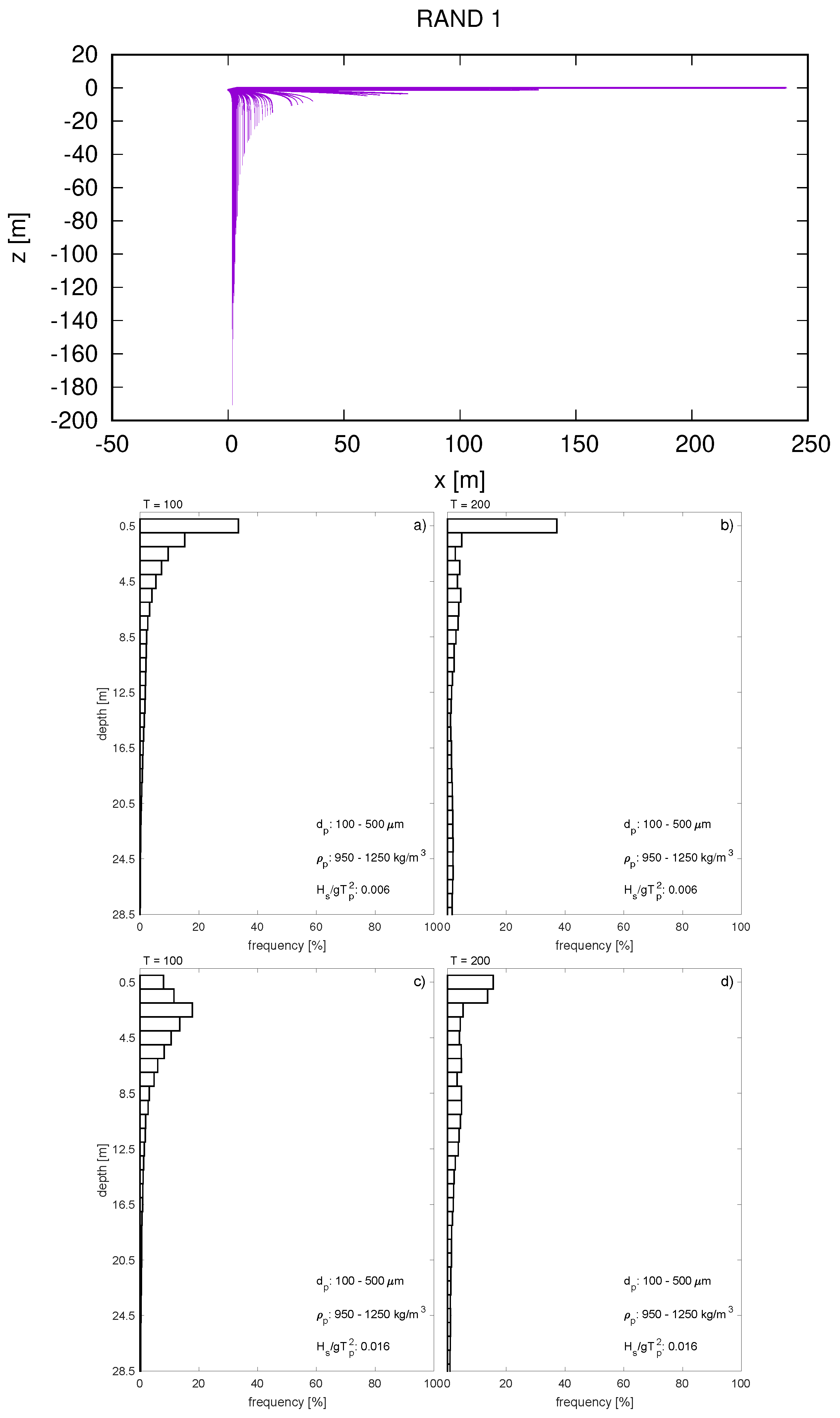
Figure 14 shows the results obtained for model sets characterized by particles with a random distribution of diameter and density. In particular, the particle diameter ranges from 100 to 500 $\mathsf{\mu }$m while the density ratio ${\rho }_p/{\rho }_f$ ranges between 0.95 and 1.25. The top panel of Figure 14 represents an example of the computed trajectories. It can be observed how, after 2000 wave periods, the particles distribute themselves along the water column with a clear separation between light particles (positively buoyant) and heavy particles (negatively buoyant). The resulting vertical frequency distribution are shown in the same figure in panels (a)–(d) for two wave parameters and two integration times, namely 100 and 200 wave periods. In this case, the frequency distributions assume a shape that is neither Gaussian-like nor uniform (as it happens for single diameter or density distributions), but tends instead to be exponentially shaped. This characteristic is most probably due to the randomness of the initial particle seeding. Higher waves tend to transport heavier particle more efficiently along the water columns, with higher percentages of particles in the lower bins (see panels (c) and (d) of Figure 14).

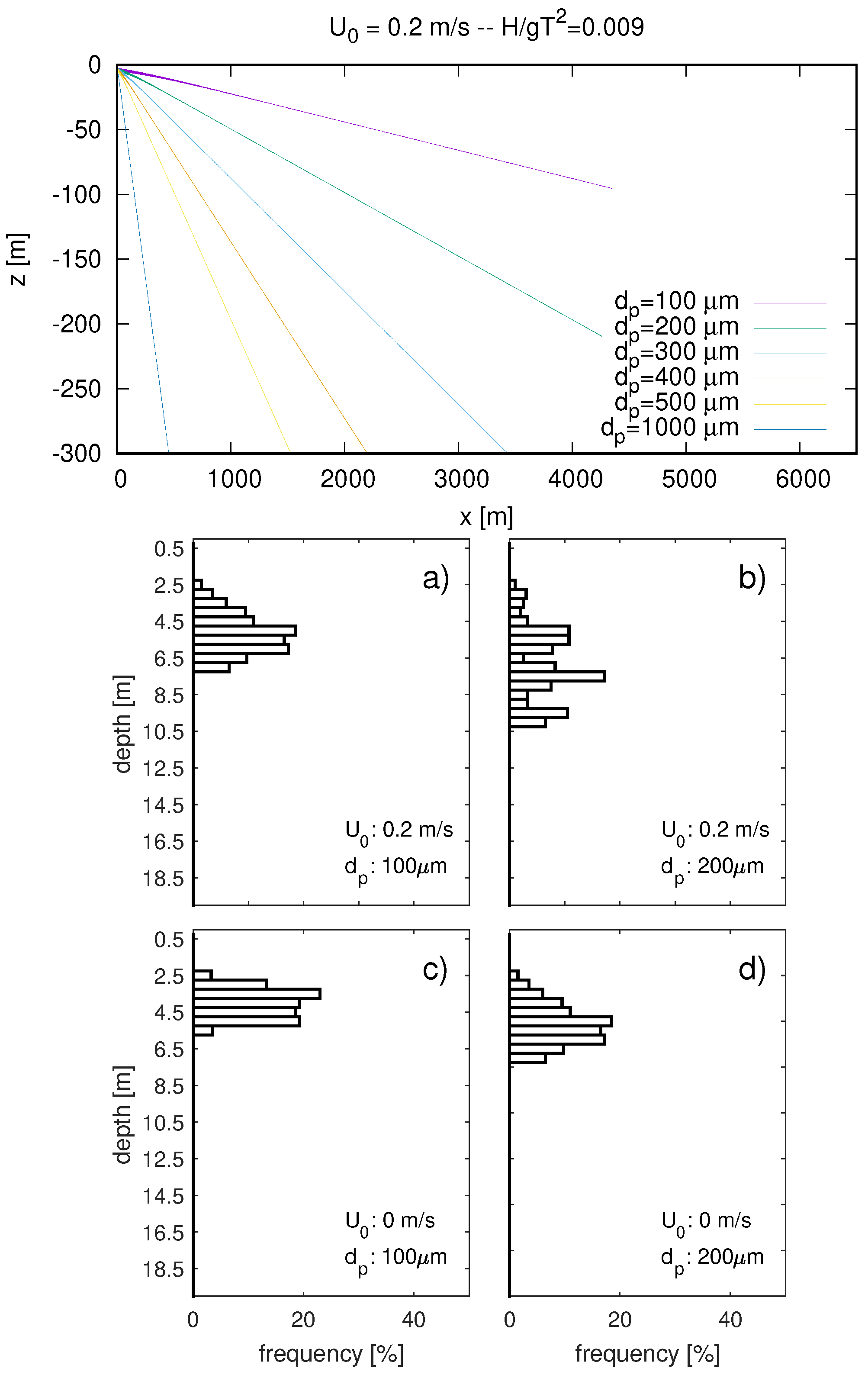
Finally, Figure 15 shows the comparison between two simulations characterized by the same wave field but under different currents (0 m/s and 0.2 m/s). The trajectories are influenced by the presence of the uniform current and a contribution proportional to the velocity is added to the particle path (top panel of Figure 15). The resulting vertical distributions are compared with those following the same environmental forcing and particle characteristics, but with no currents. The comparison between panels (a)–(b) ans panels (c)–(d) underlines how the effect of $U_0$ is observable for the larger diameters, but still not as much relevant as the other investigated parameters.

4. Discussion & Conclusions

Macro and microplastic abundance has become a fundamental information in order to determine the environmental status of a marine ecosystems. Therefore, the problem of modelling and predicting ocean microplastics pathways is being the subject of a wide literature.

The present study is primarily aimed to understand how the sea waves Stokes drift affects the dynamics of inertial micro-plastics. As for the particle inertia, this has been widely discussed in previous researches, being often taken into account in a Lagrangian framework, where the trajectory equations for passive tracer assume the following form:

$$\frac{d\mathbf{x}}{dt}=\mathbf{u}(\mathbf{x},t)$$

(10)

Since plastic generally has a different density with respect to sea water, the present study removed such hypothesis, which may be no longer reasonable especially when heavy particles are considered. Including the inertial effects extends Equation (10), leading to the trajectories expressed by Equations (4) and (5). Our results seem to suggest that, for negatively buoyant particles, (e.g., ${\rho }_p/{\rho }_f>1$), the inertial effects dominate and the resulting horizontal distance of a single particle under the effect of the sea wave drift can reach a maximum of few wavelengths (see Figure 7 and Figure 8). Therefore, it is fundamental to take into account the inertial character of the debris, as this significantly affects the paths of negatively buoyant particles. The effect of a uniform current ($U_0$) simply adds a displacement proportional to the current magnitude. On the other hand, as for plastic particles positively buoyant, the Stokes drift proves to be an effective way of transport, since the particles tend to remain in a superficial layer where the drift is more intense. In this case the residence time of plastic debris tends to increase indefinitely and, therefore, it is mandatory to consider other processes such as biofouling, which has been shown to be able to modify the density and, ultimately, the settling velocity [21,22,38]. Another aspect that require further investigations is the the time evolution of the averaged vertical velocity $\overline{w}$, which shows a transient regime characterized by an increment of the settling velocity. This can be relevant especially in shallow waters, where the combination of particles availability (e.g., sources of debris like rivers mouth etc.) and sea waves might accelerate the deposition of heavy particles. As regards the vertical distributions resulting from the trajectories computed according to Equations (4) and (5), interesting analogies with previous works can be pointed out: when random distributions for $d_p$ and ${\rho }_p$ are considered, the frequencies tend to an exponential profile that is consistent with those highlighted by Kukulka et al. [12] and Enders et al. [20], even if they relied on different models. It should be pointed out that at this stage, the model of Maxey & Riley [27] cannot be used for operational purposes. However, the second order Stokes wave represents a reasonable choice for the wave model, since its validity is not bounded by the bottom depth for common wave conditions. Then, the complexity of the marine environment implies that several more effects need to be considered, such as (but not limited to) sub-grid turbulent diffusivity, biological processes that could affect the particle properties, and non linear effects related to breaking waves [39,40].

These effects should be therefore implemented in regional models that aim to predict plastic distribution is sea basins. However, Lagrangian numerical simulations that involve inertial properties require a computational effort more severe than that needed for standard Lagrangian models for passive tracers. Indeed, the integration time step should be small compared to the Stokes time, otherwise the inertial response is not fully described. To overcome this limitation, it would be desirable a closure model, able to represent inertial effect through an effective diffusivity in analogy to the standard closures for turbulent transport coefficient.

Finally, is is worth to mention that laboratory experiments are needed to further test the reliability of the analytical model. To this end, an experimental campaign has been recently kicked off at the Department of Civil, Chemical and Environmental Engineering of the University of Genoa, and will be the focus of a future publication.

References

- Thompson, R.C.; Swan, S.H.; Moore, C.J.; Vom Saal, F.S. Our Plastic Age. Philos. Trans. R. Soc. B 2009. [Google Scholar] [CrossRef] [PubMed] [Green Version]
- Wilson, D.C.; Rodic, L.; Modak, P.; Soos, R.; Carpintero, A.; Velis, K.; Iyer, M.; Simonett, O. Global Waste Management Outlook; UNEP: Nairobi, Kenya, 2015. [Google Scholar]
- Jambeck, J.R.; Geyer, R.; Wilcox, C.; Siegler, T.R.; Perryman, M.; Andrady, A.; Narayan, R.; Law, K.L. Plastic waste inputs from land into the ocean. Science 2015, 347, 768–771. [Google Scholar] [CrossRef] [PubMed]
- Derraik, J.G. The pollution of the marine environment by plastic debris: A review. Mar. Pollut. Bull. 2002, 44, 842–852. [Google Scholar] [CrossRef]
- Kershaw, P.; Rochman, C. Sources, fate and effects of microplastics in the marine environment: Part 2 of a global assessment. In Reports and studies-IMO/FAO/Unesco-IOC/WMO/IAEA/UN/UNEP Joint Group of Experts on the Scientific Aspects of Marine Environmental Protection (GESAMP) Eng No. 93; International Maritime Organization: London, UK, 2015. [Google Scholar]
- Van Sebille, E.; Wilcox, C.; Lebreton, L.; Maximenko, N.; Hardesty, B.D.; Van Franeker, J.A.; Eriksen, M.; Siegel, D.; Galgani, F.; Law, K.L. A global inventory of small floating plastic debris. Environ. Res. Lett. 2015, 10, 124006. [Google Scholar] [CrossRef]
- Hidalgo-Ruz, V.; Gutow, L.; Thompson, R.C.; Thiel, M. Microplastics in the marine environment: A review of the methods used for identification and quantification. Environ. Sci. Technol. 2012, 46, 3060–3075. [Google Scholar] [CrossRef]
- Bec, J. Fractal clustering of inertial particles in random flows. Phys. Fluids 2003, 15, L81–L84. [Google Scholar] [CrossRef] [Green Version]
- Maximenko, N.; Hafner, J.; Niiler, P. Pathways of marine debris derived from trajectories of Lagrangian drifters. Mar. Pollut. Bull. 2012, 65, 51–62. [Google Scholar] [CrossRef]
- Zambianchi, E.; Trani, M.; Falco, P. Lagrangian transport of marine litter in the Mediterranean Sea. Front. Environ. Sci. 2017, 5, 5. [Google Scholar] [CrossRef] [Green Version]
- Ballent, A.; Purser, A.; de Jesus Mendes, P.; Pando, S.; Thomsen, L. Physical transport properties of marine microplastic pollution. Biogeosci. Discuss. 2012, 9. [Google Scholar] [CrossRef] [Green Version]
- Kukulka, T.; Proskurowski, G.; Morét-Ferguson, S.; Meyer, D.; Law, K. The effect of wind mixing on the vertical distribution of buoyant plastic debris. Geophys. Res. Lett. 2012, 39. [Google Scholar] [CrossRef] [Green Version]
- Kukulka, T.; Brunner, K. Passive buoyant tracers in the ocean surface boundary layer: 1. Influence of equilibrium wind-waves on vertical distributions. J. Geophys. Res. Oceans 2015, 120, 3837–3858. [Google Scholar] [CrossRef]
- Isobe, A.; Kubo, K.; Tamura, Y.; Kako, S.; Nakashima, E.; Fujii, N. Selective transport of microplastics and mesoplastics by drifting in coastal waters. Mar. Pollut. Bull. 2014, 89, 324–330. [Google Scholar] [CrossRef] [PubMed]
- Liubartseva, S.; Coppini, G.; Lecci, R.; Creti, S. Regional approach to modeling the transport of floating plastic debris in the Adriatic Sea. Mar. Pollut. Bull. 2016, 103, 115–127. [Google Scholar] [CrossRef]
- Zhang, H. Transport of microplastics in coastal seas. Estuar. Coast. Shelf Sci. 2017, 199, 74–86. [Google Scholar] [CrossRef]
- Liubartseva, S.; Coppini, G.; Lecci, R.; Clementi, E. Tracking plastics in the Mediterranean: 2D Lagrangian model. Mar. Pollut. Bull. 2018, 129, 151–162. [Google Scholar] [CrossRef]
- Ourmieres, Y.; Mansui, J.; Molcard, A.; Galgani, F.; Poitou, I. The boundary current role on the transport and stranding of floating marine litter: The French Riviera case. Cont. Shelf Res. 2018, 155, 11–20. [Google Scholar] [CrossRef] [Green Version]
- Jalón-Rojas, I.; Wang, X.H.; Fredj, E. On the importance of a three-dimensional approach for modelling the transport of neustic microplastics. Ocean Sci. 2019, 15, 717–724. [Google Scholar] [CrossRef] [Green Version]
- Enders, K.; Lenz, R.; Stedmon, C.A.; Nielsen, T.G. Abundance, size and polymer composition of marine microplastics greater then 10 μm in the Atlantic Ocean and their modelled vertical distribution. Mar. Pollut. Bull. 2015, 100, 70–81. [Google Scholar] [CrossRef]
- Kooi, M.; van Nes, E.H.; Scheffer, M.; Koelmans, A.A. Ups and downs in the ocean: effects of biofouling on vertical transport of microplastics. Environ. Sci. Technol. 2017, 51, 7963–7971. [Google Scholar] [CrossRef] [Green Version]
- Porter, A.; Lyons, B.P.; Galloway, T.S.; Lewis, C.N. The role of marine snows in microplastic fate and bioavailability. Environ. Sci. Technol. 2018. [Google Scholar] [CrossRef]
- Arthur, C.; Baker, J.E.; Bamford, H.A. Proceedings of the International Research Workshop on the Occurrence, Effects, and Fate of Microplastic Marine Debris; University of Washington Tacoma: Tacoma, WA, USA, 2009. [Google Scholar]
- Rios, L.M.; Moore, C.; Jones, P.R. Persistent organic pollutants carried by synthetic polymers in the ocean environment. Mar. Pollut. Bull. 2007, 54, 1230–1237. [Google Scholar] [CrossRef]
- Fossi, M.C.; Panti, C.; Guerranti, C.; Coppola, D.; Giannetti, M.; Marsili, L.; Minutoli, R. Are baleen whales exposed to the threat of microplastics? A case study of the Mediterranean fin whale (Balaenoptera physalus). Mar. Pollut. Bull. 2012, 64, 2374–2379. [Google Scholar] [CrossRef]
- Peregrine, D. Interaction of water waves and currents. In Advances in Applied Mechanics; Elsevier: Amsterdam, The Netherlands, 1976; Volume 16, pp. 9–117. [Google Scholar]
- Maxey, M.R.; Riley, J.J. Equation of motion for a small rigid sphere in a nonuniform flow. Phys. Fluids 1983, 26, 883–889. [Google Scholar] [CrossRef]
- Santamaria, F.; Boffetta, G.; Afonso, M.M.; Mazzino, A.; Onorato, M.; Pugliese, D. Stokes drift for inertial particles transported by water waves. EPL (Europhys. Lett.) 2013, 102, 14003. [Google Scholar] [CrossRef] [Green Version]
- DiBenedetto, M.H.; Ouellette, N.T.; Koseff, J.R. Transport of anisotropic particles under waves. J. Fluid Mech. 2018, 837, 320–340. [Google Scholar] [CrossRef]
- Khatmullina, L.; Isachenko, I. Settling velocity of microplastic particles of regular shapes. Mar. Pollut. Bull. 2017, 114, 871–880. [Google Scholar] [CrossRef]
- Mentaschi, L.; Besio, G.; Cassola, F.; Mazzino, A. Developing and validating a forecast/hindcast system for the Mediterranean Sea. J. Coast. Res. 2013, 65, 1551–1556. [Google Scholar] [CrossRef]
- Mentaschi, L.; Besio, G.; Cassola, F.; Mazzino, A. Problems in RMSE-based wave model validations. Ocean Model. 2013, 72, 53–58. [Google Scholar] [CrossRef]
- Mentaschi, L.; Besio, G.; Cassola, F.; Mazzino, A. Performance evaluation of WavewatchIII in the Mediterranean Sea. Ocean Model. 2015, 90, 82–94. [Google Scholar] [CrossRef]
- LeMéhauté, B. An Introduction to Hydrodynamics and Water Waves; Springer: Berlin, Germany, 1976. [Google Scholar]
- Chubarenko, I.; Bagaev, A.; Zobkov, M.; Esiukova, E. On some physical and dynamical properties of microplastic particles in marine environment. Mar. Pollut. Bull. 2016, 108, 105–112. [Google Scholar] [CrossRef]
- Kooi, M.; Reisser, J.; Slat, B.; Ferrari, F.F.; Schmid, M.S.; Cunsolo, S.; Brambini, R.; Noble, K.; Sirks, L.A.; Linders, T.E.; et al. The effect of particle properties on the depth profile of buoyant plastics in the ocean. Sci. Rep. 2016, 6, 33882. [Google Scholar] [CrossRef] [Green Version]
- Kumar, N.; Cahl, D.L.; Crosby, S.C.; Voulgaris, G. Bulk versus spectral wave parameters: Implications on stokes drift estimates, regional wave modeling, and HF radars applications. J. Phys. Oceanogr. 2017, 47, 1413–1431. [Google Scholar] [CrossRef] [Green Version]
- Kaiser, D.; Kowalski, N.; Waniek, J.J. Effects of biofouling on the sinking behavior of microplastics. Environ. Res. Lett. 2017, 12, 124003. [Google Scholar] [CrossRef] [Green Version]
- Deike, L.; Pizzo, N.; Melville, W.K. Lagrangian transport by breaking surface waves. J. Fluid Mech. 2017, 829, 364–391. [Google Scholar] [CrossRef] [Green Version]
- Pizzo, N.; Melville, W.K.; Deike, L. Lagrangian Transport by Nonbreaking and Breaking Deep-Water Waves at the Ocean Surface. J. Phys. Oceanogr. 2019, 49, 983–992. [Google Scholar] [CrossRef]
Figure 1.
Geographical location of hindcast points used to set the wave parameters for the present study.
Figure 2.
Each row corresponds to a single reanalysis point among those indicated in Figure 1. Left column: wave period T versus wave height H, colormap indicates the number of events encountered in the time frame of the meteocean hindcast; right column: histograms of the dimensionless parameter having set a threshold on the wave height equal to 0.3 m.
Figure 3.
Example of numerical trajectories for a series of simulations with increasing RUN 12: 0.001; RUN 13: 0.002; RUN 16: 0.005; RUN 17: 0.007 (cfr. Table 1). The plots correspond to runs with a fixed density ratio and for several particle diameter . The duration of the simulations are about 3000 wave periods.
Figure 4.
Close up of the trajectories of RUN12 for the larger diameters.
Figure 5.
Example of numerical trajectories for a series of simulations with increasing . RUN 12: 0.001; RUN 13: 0.002; RUN 16: 0.005; RUN 17: 0.007 (cfr. Table 1). The plots correspond to runs with a fixed value of the particle diameter = 100 m and for several density ratio. The duration of the simulations are about 3000 wave periods.
Figure 6.
Normalized maximum horizontal distance as a function of . Each panel corresponds to a series of experiments with fixed wave period, wave length and density ratio and varying wave amplitude and particle diameter.
Figure 7.
Normalized maximum horizontal distance as a function of the Stokes number and wave parameter , for a fixed density ratio . The plot is in log-log scales. The theoretical curve of [28] is reported for a single number just to highlight the functional dependence between and .
Figure 8.
Normalized maximum horizontal distance as a function of the added-mass parameter . The curves represent a series of experiments with fixed wave period, wave length and particle diameter and varying wave amplitude and .
Figure 9.
Time evolution of the vertical velocity for different particle diameter: (a) = 100 m; (b) = 500 m; (c) = 700 m; (d) = 1000 m. Wave parameter .
Figure 10.
Time evolution of the normalized period averaged vertical velocity for different particle diameter at fixed wave parameter .
Figure 11.
Vertical distribution of plastic particles for experiments with fixed particle density ( kg/m) and fixed wave field ( ) and varying particle sizes: (a) = 200 m; (b) = 400 m; (c) = 600 m; (d) = 1000 m. Vertical profiles are taken after 100 wave periods.
Figure 12.
Vertical distribution of plastic particles for experiments with fixed particle size ( = 100 m) and fixed wave field () and varying density ratio: (a) kg/m; (b) kg/m; (c) kg/m; (d) kg/m. Vertical profiles are taken after 200 wave periods.
Figure 13.
Vertical distribution of plastic particles for experiments with fixed particle density ( kg/m) and fixed particle size ( =100 m) and varying sea wave state. Top panels: ; (a) after 100 T; (b) after 500 T; (c) after 1000. Middle panels: ; (d) after 100 T; (e) after 500 T; (f) after 1000 T. Bottom panels: (g) after 100 T; (h) after 500 T; (i) after 1000 T.
Figure 14.
Top panel: Example of numerical trajectories for a random distribution of particles, ranging from 100 to 500 m and ranging between 0.95 and 1.25. Vertical distribution of plastic particles obtained for the experiments rand1 () and rand4 () after 100 wave periods panel (a) and (c) and 200 wave periods panel (b) and (d).
Figure 15.
Top panel: Example of numerical trajectories simulated for particle of different sizes and constant density ratio showing the effect of a uniform current m/s and . Bottom panels: comparison of frequency distribution for the same wave, for two particle diameter, for a run with the uniform flow, panels (a,b) and without current panels (c,d). Integration time equal to 100 T.