Quantifying the Spatio-Temporal Process of Township Urbanization: A Large-Scale Data-Driven Approach

Key Laboratory of Agro-Ecological Processes in Subtropical Region and Changsha Research Station for Agricultural& Environmental Monitoring, Institute of Subtropical Agriculture, Chinese Academy of Sciences, Changsha 410125, China
*
Author to whom correspondence should be addressed.
ISPRS Int. J. Geo-Inf. 2019, 8(9), 389; https://doi.org/10.3390/ijgi8090389
Submission received: 26 July 2019
/
Revised: 31 August 2019
/
Accepted: 2 September 2019
/
Published: 4 September 2019
Abstract
:The integrated recognition of spatio-temporal characteristics (e.g., speed, interaction with surrounding areas, and driving forces) of urbanization facilitates regional comprehensive development. In this study, a large-scale data-driven approach was formed for exploring the township urbanization process. The approach integrated logistic models to quantify urbanization speed, partial triadic analysis to reveal dynamic relationships between rural population migration and urbanization, and random forest analysis to identify the response of urbanization to spatial driving forces. A typical subtropical town was chosen to verify the approach by quantifying the spatio-temporal process of township urbanization from 1933 to 2012. The results showed that (i) urbanization speed was well reflected by the changes of time-course areas of urban cores fitted by a four-parameter logistic equation (R2 = 0.95–1.00, p < 0.001), and the relatively fast and steady developing periods were also successfully predicted, respectively; (ii) the spatio-temporal sprawl of urban cores and their interactions with the surrounding rural residential areas were well revealed and implied that the town experienced different historically aggregating and splitting trajectories; and (iii) the key drivers (township merger, elevation and distance to roads, as well as population migration) were identified in the spatial sprawl of urban cores. Our findings proved that a comprehensive approach is powerful for quantifying the spatio-temporal characteristics of the urbanization process at the township level and emphasized the importance of applying long-term historical data when researching the urbanization process.
1. Introduction
Urbanization presents complicated processes and presents multiple spatio-temporal characteristics, e.g., urbanization speed, reciprocal relations with surrounding rural areas, and spatial sprawl. Meanwhile, the urban system includes several hierarchical levels, i.e., urban clusters, provincial capital cities, prefectural-level cities, county-level cities, and towns or villages [1,2,3,4]. Compared with large cities’ urbanization, township urbanization exhibits more direct impacts on biodiversity reduction and arable land change [2,3]. However, to date, most urban research has focused on big cities [5,6], and these researching theories and frameworks of urbanization processes cannot be directly applied in township urbanization studies [7]. Therefore, it is necessary to form unique techniques and frameworks to detect and predict the spatio-temporal developing characteristics of the urbanization process at the town scale.
The level or speed of urbanization is a prerequisite aspect of studying urban development, while the concepts and measuring methods are still in controversy [3,8,9]. Due to the constant change of urban areas and the conflicting statistics on urban population during several censuses, there was no solid foundation for researchers to compare the urbanization levels at different times. Moreover, even if on the basis of the same national census, there was no way to compare urbanization levels in different areas [2,7]. In order to address the above problems, a population urbanization-level index was constructed based on factors such as population, economy, society, and living environment [10]. Despite significant advances in the development of the quantifying the level and speed of urbanization across the science and policy arenas, an accurate and comprehensive evaluation of urban development remains challenging, especially at the town scale and in data-scarce regions [10,11]. According to the literature, the spatial change of a town center pattern was the most intuitive expression of urbanization at the town scale, and ordinarily showed a significantly positive correlation with socio-economic development [2,12]. Several studies selected change of town center pattern as an important urbanization indicator for exploring the impact of urbanization on ecosystem services deterioration, arable land loss, and agricultural landscape fragments [8,13]. Thus, this study introduced the spatio-temporal changes of urban cores to reflect the township urbanization process.
Township urbanization presents close correlation with surrounding rural residences [8]. Exploring urban spatial pattern and its interaction with the surrounding environment in a rapidly urbanizing region can contribute significantly to the quantifying, monitoring, and understanding of the complex urbanization process [14,15,16,17]. Because urban systems are multi-scaled and social-ecological systems, a comprehensive approach is needed for understanding their structure, function, and dynamic interaction with the surrounding residential area [4,14]. Moreover, the increment of urban populations, the expansion of urban built-up areas, and the changes of urban environments were considered as key aspects of transformation for the urbanization process [2,9]. For the systemic research of the urbanization process, some urban developing theories, e.g., the diffusion–coalescence and spatial heterogeneity hypothesis, were used to demonstrate the spatio-temporal relationships between the urban cores and the surrounding residential areas [4]. However, exploring and mapping such an urbanization process is a challenging task, due to the issues of spatial heterogeneity and dynamic land-use practices [18,19,20]. In this study, landscape index and spatio-temporal statistical method were used to explore urban patterns and the dynamic relationship between urban cores and surrounding residential areas.
The spatio-temporal driving mechanism of urbanization has always been a focus for the academic community [12,21,22]. Current theories mainly address population moving and relocation, economic explanations, transport and communication, policies, and institutions [2,23]. Moreover, certain biophysical driving forces with spatial heterogeneity have been found to be the essential components for influencing the urbanization process [15,24,25]. Several studies also demonstrated that industrialization and structural transition of rural laborers were the main driving forces to promote urbanization [2,3]. For instance, the economic reform has been gradually launched in extensive rural areas in China, resulting in a large amount of agriculture surplus laborers who gradually moved into adjacent urban cores [1,3]. Township enterprises are flourishing and are becoming the leading factor for promoting rural urbanization [2,7,11]. Numerous studies have been devoted to finding subsets of measures, including demographic factors, physical variables, and landscape metrics [2,4,15,22]. Such sets of measures play important roles in the facilitation of comprehensive understandings of urban ecology and allow researchers to directly compare diverse urban areas across the globe [3,26,27]. Thus, social, policy, demographic, and physical determinants of the urbanization process were integrated and analyzed in this study.
For quantifying the spatio-temporal urbanization process at the township level, a large-scale data driven approach was established, and a representative town (Jinjing) was chosen to verify the approach, which typifies many towns in terms of geo-morphology and socio-economic dynamics, making it an ideal microcosm of the larger region. In general, similarly to a higher-level administrative unit, a town includes at least one urban core, which can be considered the center of the town and the mark of urbanization [12]. Exploring the characteristics and processes of urbanization at the town scale should provide critical references for land planners creating policies and strategies for future urban development. Therefore, urban cores were extracted to investigate their growth characteristics and processes at the town scale. The primary objectives of this study were (i) to develop a set of analytical methods to facilitate urban cores research at the town scale; (ii) to investigate the spatio-temporal development processes of the urban cores at the town scale; (iii) to quantify the spatio-temporal relationships between urban cores growth and surrounding settlements migration; and (iv) to analyze the driving forces of urban cores development at the town scale.
2. Materials and Methods
2.1. Methodology
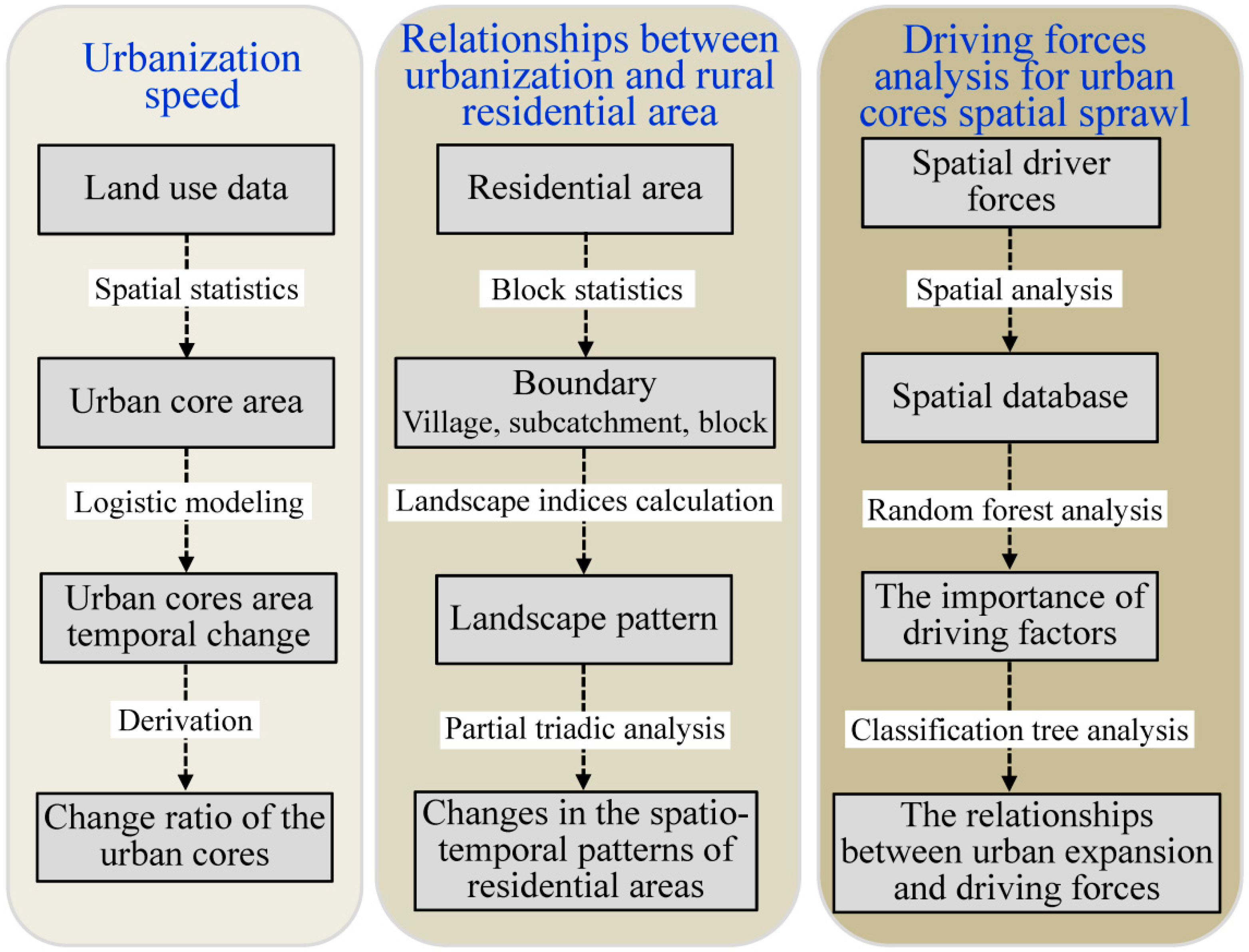
A methodological flow chart for a systemic view is provided in Figure 1. It involves three major steps: (1) quantifying urbanization speed by employing logistic models; (2) analyzing relationships between urbanization and the rural residential area by using landscape indices and partial triadic analysis (PTA); and (3) identifying driving forces for spatial sprawl of urban cores by applying random forest (RF) and classification tree analysis (CTA).
2.1.1. Logistic Models
Two logistic models, i.e., a three-parameter logistic equation (3PL) and a four-parameter logistic equation (4PL), were used to describe the development of urban cores. The two logistic models can be described as follows: 3PL (Equation (1)), as a typical model, has been widely used to simulate urban development. The derivation (Equation (2)) of 3PL was used to present the change ratio of urban cores.
where x is the urban area, t is the time (years) of urban area change, k characterizes the slope of the curve at its midpoint, xm is the maximum area of the urban core (top of the curve), and x0 is the minimum area of the urban core (bottom of the curve).
In contrast to 3PL, 4PL (Equation (3)) is a typical dose-response curve with a variable slope parameter. The derivation (Equation (4)) of 4PL was used to present the change ratio of the urban cores.
where t2 is the t value for the curve point that is midway between the xm and x0 parameters, also called the half-maximal effective time.
For the two logistical methods, 95% confidence intervals were used to evaluate their fitted effect and calculated by Monte Carlo simulation with 10,000 simulations. The root mean square error (RMSE) and coefficient of determination (R2) of the linear regression between the observed and predicted values were used as the two indicators of model fit. In this study, R software and the nls2 package were used to fit and evaluate the logistic models [27].
2.1.2. Landscape Index and Partial Triadic Analysis
The landscape index analysis and PTA were used to reveal the dynamic relationships between the urbanization process and the surrounding rural residences. Landscape indices, including the patch area_mean (AREA_MN), patch cohesion index (COHESION), contiguity index mean (CONTIG_MN), fractal dimension index mean (FRAC_MN), largest patch index (LPI), effective mesh size (MESH), shape index mean (SHAPE_MN), and splitting index (SPLIT), were calculated and used as the necessary input data for the PTA. Details regarding these landscape indices are presented in Table 1. R software (http://www.r-project.org) and Fragstats software were used to calculate the landscape indices.
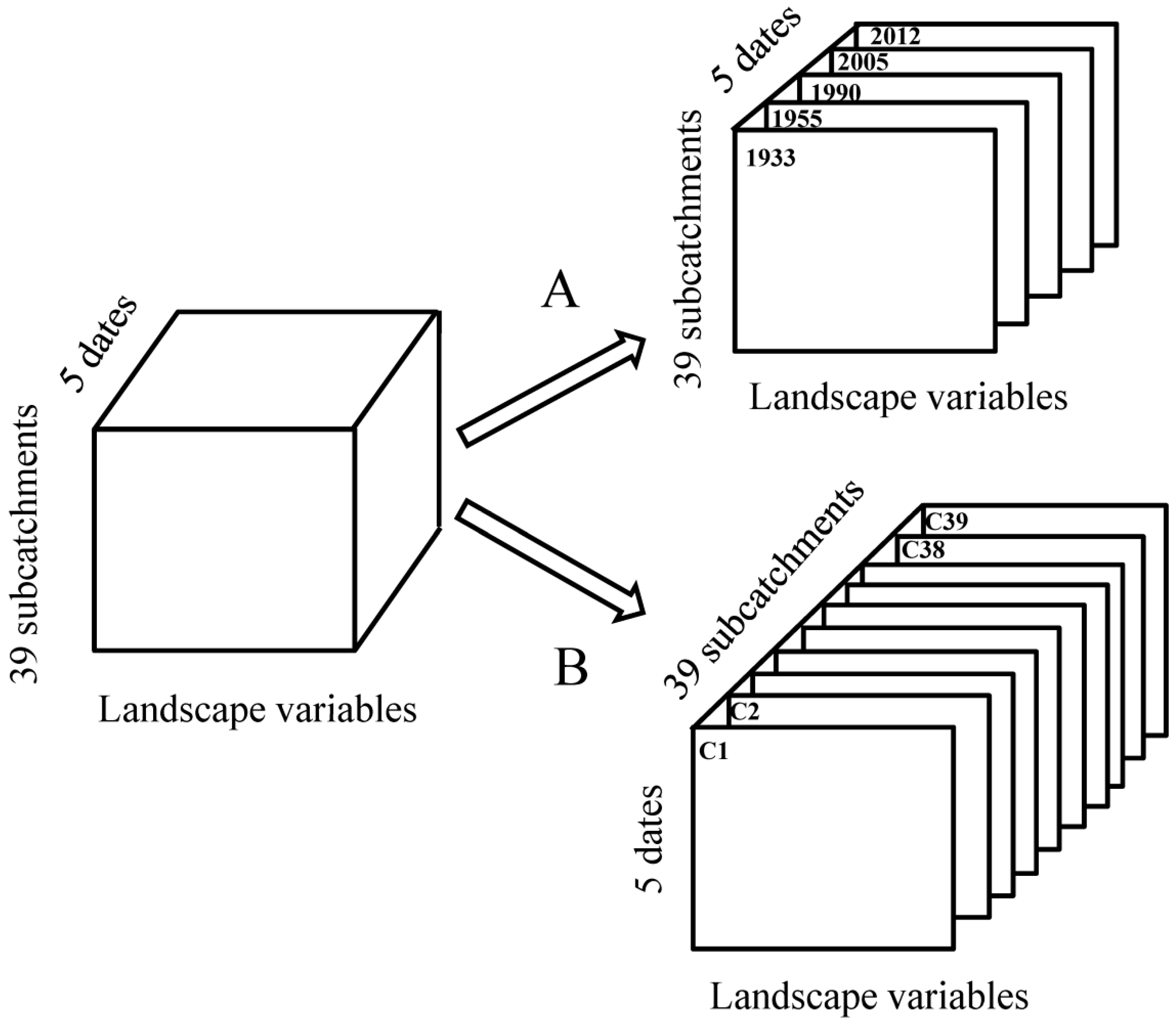
PTA is based on the logic of principal components analysis and the aim is to analyze a three-dimensional table (i.e., in this study, a data cube: Landscape indices × catchments × years) presented as a sequence of two-dimensional tables (i.e., landscape indices ×catchments) (Figure 2). The PTA and graphic preparations were performed using the R package ade4 [28,29].
2.1.3. Classification Tree Analysis and Random Forest Analysis
Descriptive statistics were analyzed to determine social and policy driving forces, e.g., population and township mergers. The influence of spatial driving forces, e.g., elevation, slope, aspect, distance to rivers (dis_rivers), distance to roads (dis_roads), and distance to lakes (dis_lakes), was analyzed by classification tree analysis (CTA) and random forest (RF) analysis. For these two analyses, all urban core cells in each map were set to a value of 1, while the rest of the cells were set to 0. R statistical software and the Random Forests [30] and rpart [31] packages were employed for the data analysis. CTA was applied to develop and plot the regression trees in order to describe the relationships between urban expansion and its driving forces. No assumptions were made about the relationships between urban expansion and its driving forces, and the relationships and formed clusters were modeled by repeatedly splitting the data, with each split chosen to minimize the dissimilarity within clusters [32]. A regression tree is a forecasting tree-like diagram resulting from recursively partitioning the response data, with indication of the influence of the explanatory variables at each split. RF analysis was used to evaluate the importance of driving factors related to the spatial distribution, where the value can be between 0 and 1, with a value closer 1 indicating a stronger influence. The analysis provides an ensemble classification method that consists of many regression trees developed by CTA and that outputs the class that is the mean prediction of individual trees [33]. For detailed descriptions of CTA and RF analysis, refer to http://www.r-project.org.
2.2. Data Acquisition and Processing
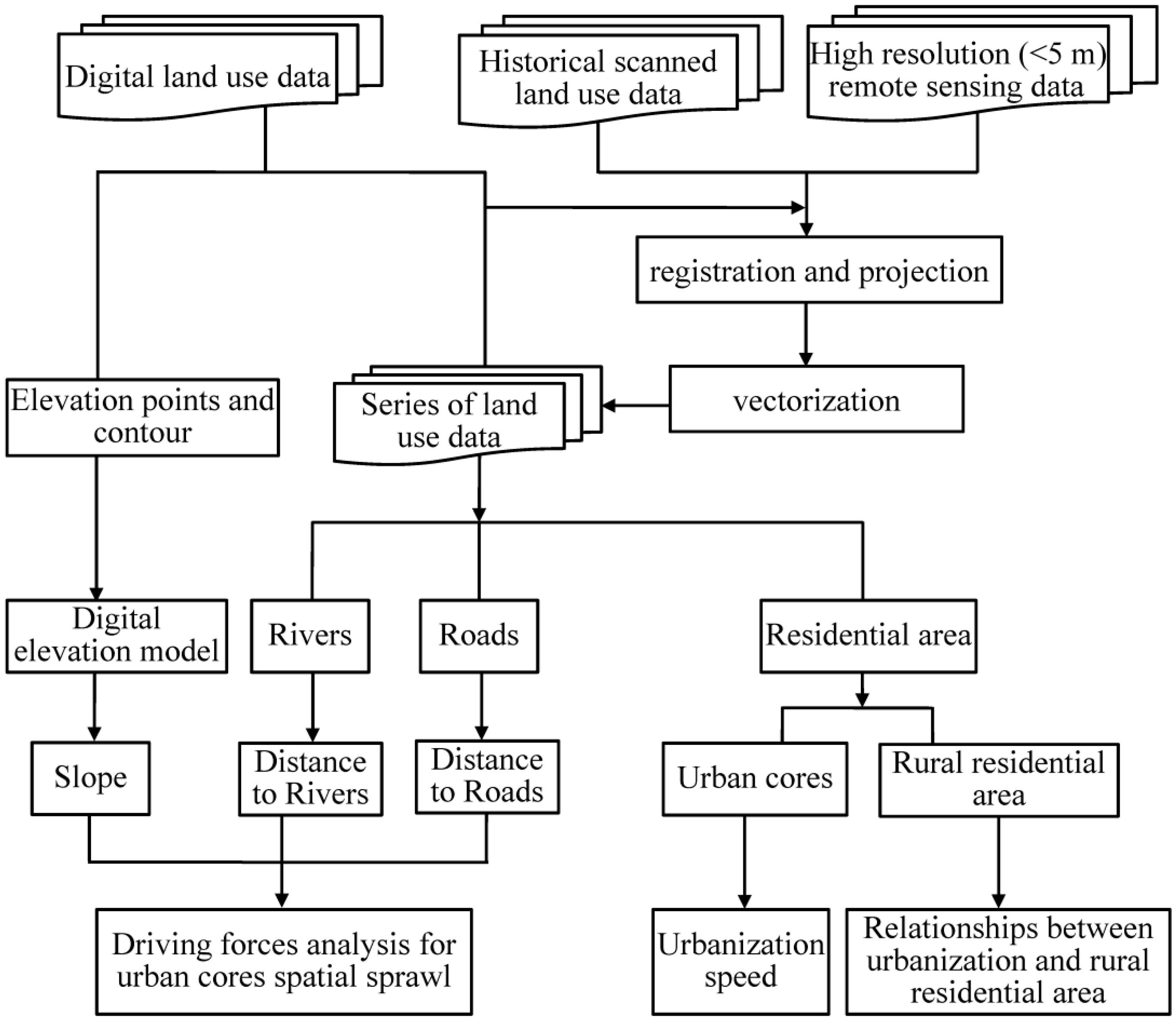
A data acquiring and processing flow chart is provided in Figure 3. Original data types mainly include digital land-use data, historical scanned land-use data, and high resolution (<5 m) remote sensing data. The format of digital land-use data is usually E00 or coverage and could be converted to a shapefile format. Historical scanned land-use data is the scanning electronic version of historical archives and used to acquire historical land-use data before the appearance of high-resolution remote sensing data. High resolution (<5 m) remote sensing data includes satellite (quikbird, SPOT, World View, and GeoEye-1) data, Google maps, and air photographs, which should satisfy the requirement of interpreting individual residential land. After registration and projection, the above data were vectorized to obtain a series of land-use data and then extract residential area, rivers and roads for quantifying the spatio-temporal growth of urban cores at the township level.
2.3. Study Area
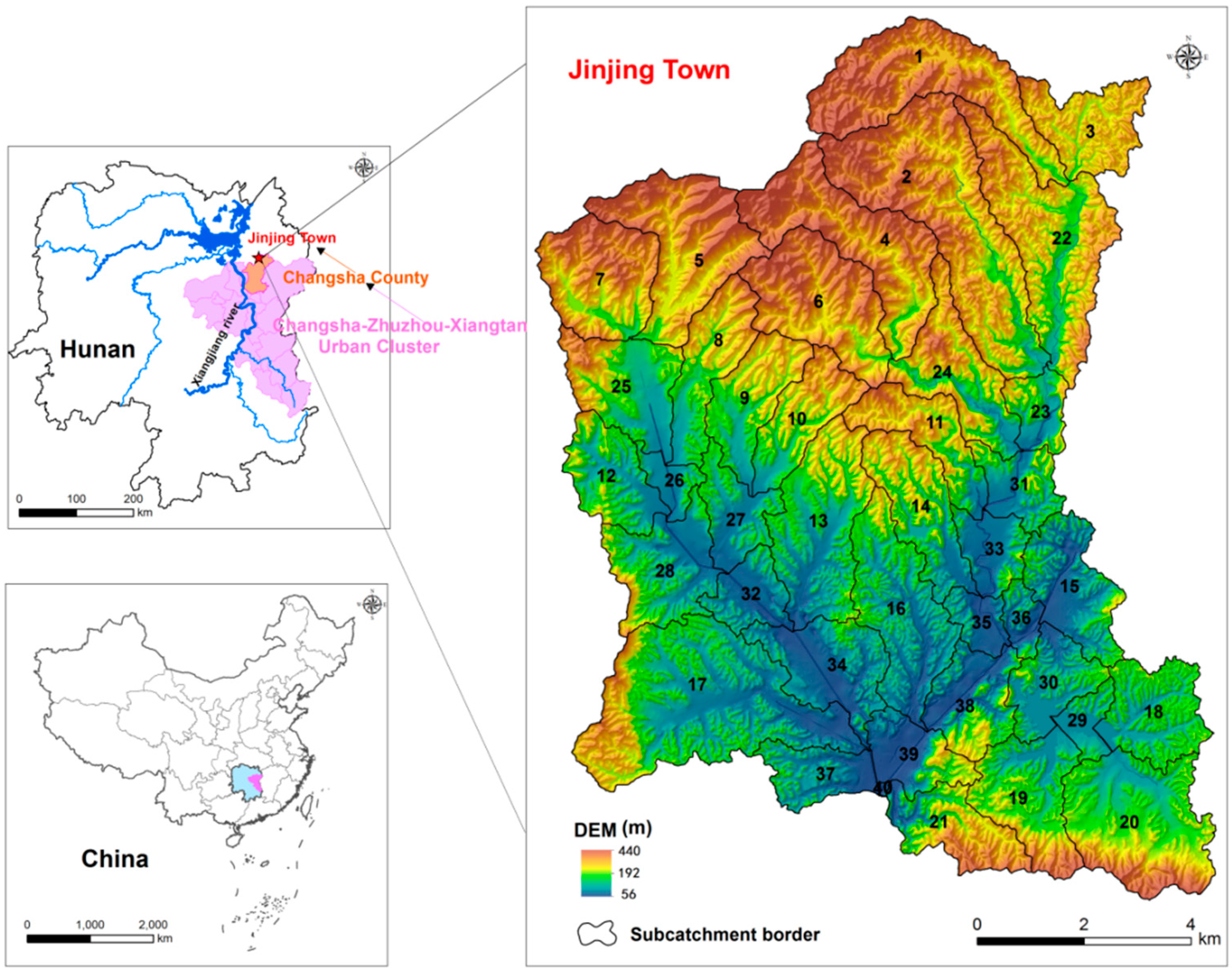
Jinjing Town is located in the northeast of the Changsha–Zhuzhou–Xiangtan urban cluster (also named the Greater Changsha Metropolitan Region), which has been appraised as “China’s first experimental case of conscious regional economic integration” [2], and it is a heavily urbanized region that has greatly promoted economic development in Central China. Jinjing Town has a population of 42,080 people (2018) and an area of 135 km2 (Figure 4). The main land use types area are woodlands (56%) and paddy fields (34%), and the dominant crops include rich (prolific) rice, tea, and various vegetables (e.g., snap been, water spinach, cabbage, and cauliflower) [8]. The history of the study area can be divided into four major periods. The first period was prior to the foundation of the People’s Republic of China in 1949. Only a few people lived in the area due to consecutive years of war, and urban cores were not formed. The second period lasted from 1949 to 1978, the population increased by a factor of more than eight, and urban cores were formed and rapidly developed. The third period began in 1978 and the tea industry has been flourishing and bringing considerable economic benefits to Jinjing Town. The study area has been undergoing the fourth urban development period since 1991, since there was at ownship merger where two adjacent towns (Tuojia and Guanjia) were merged into Jinjing Town. The newly created town was named Jinjing, and the original two towns (Tuojia and Guanjia) were reorganized as two villages of Jinjing Town (http://jjz.csx.cn/).
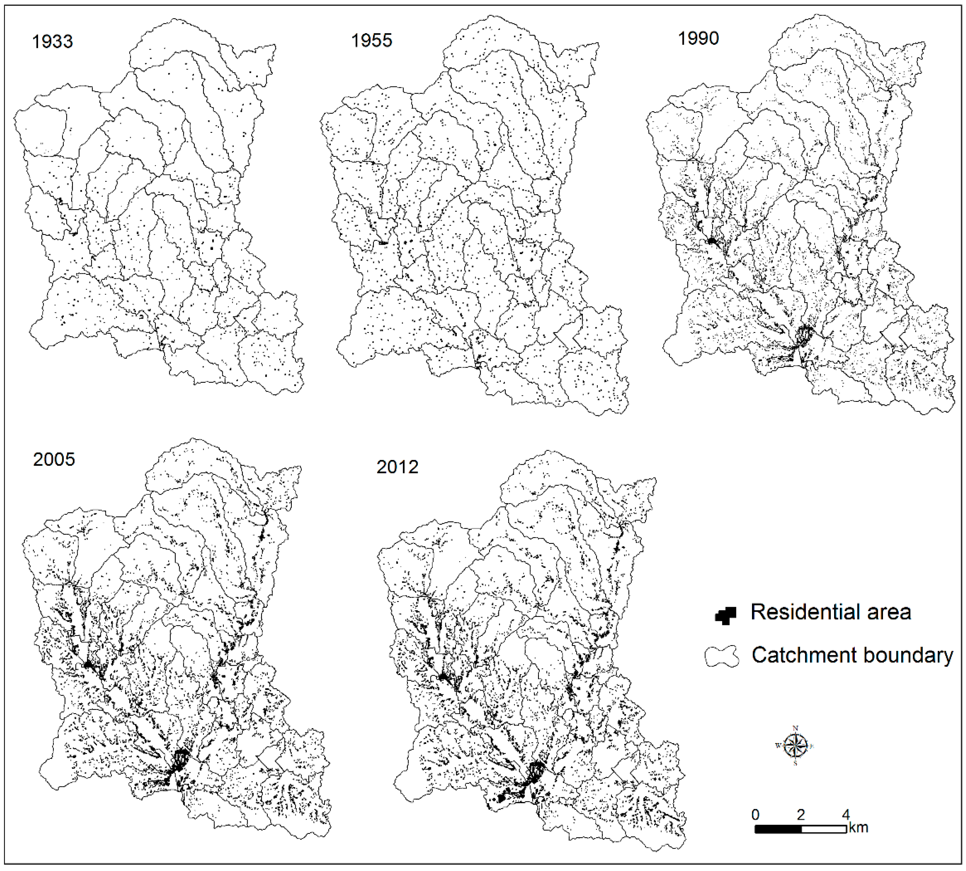
In this study, data on the residential distribution for five years (i.e., 1933, 1955, 1990, 2005, and 2012) were used to investigate the spatio-temporal pattern of urbanization in Jinjing Town (Figure 5). Data for 1933, 1955, and 1990 were extracted from the historical topographic maps (scale 1:10,000) obtained from the Hunan Province Geomatics Information Center (http://www.hnpgc.com). The extraction process included scanning historical maps by using CONTEX HD Ultra i4450s and performing image rectification and vectorization in ArcGIS 10.0. Data for 2005 were extracted from a digital topographic map that included elevation information (points and contours) and land-use data (woodlands, paddy fields, tea fields, roads, residential areas, and water bodies). The elevation information was used to generate a digital elevation model (DEM) at a 5 m resolution by using the “Topo to Raster” function in ArcGIS 10.0. Data for 2012 were vectorized from an air photograph (at a 2 m resolution) taken by airplane on 14 June 2012.
In a hilly area such as Jinjing Town, the distribution of residents is significantly influenced by topography and, thus, the administrative boundary is nearly on the ridgelines. To explore the spatio-temporal changes of settlements, Jinjing Town was divided into 39 catchments using the Hydrology Analysis extension of ArcGIS 10.2 based on the DEM (Figure 4).
3. Results
3.1. Urbanization Speed
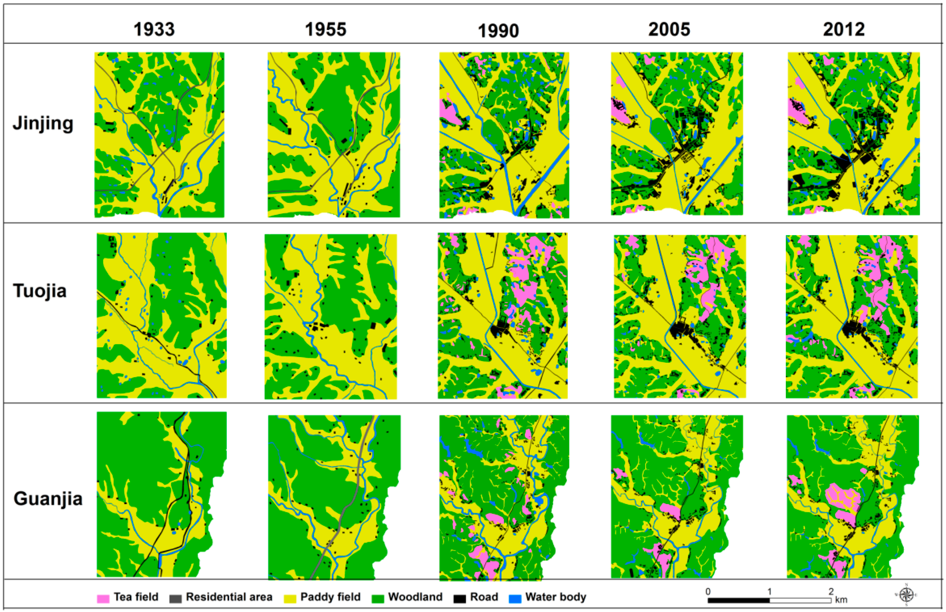
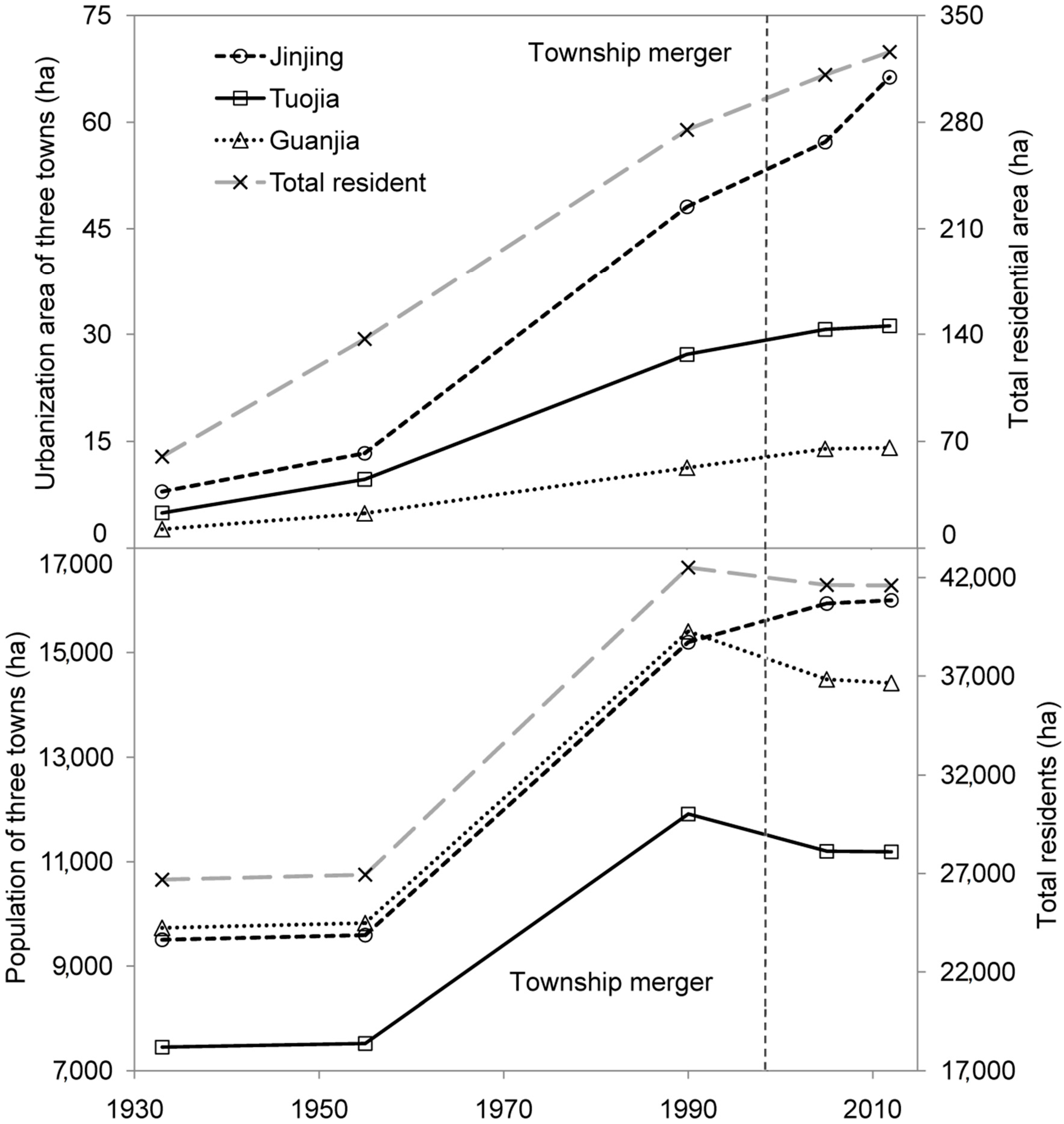
The changes in the spatio-temporal patterns of the three urban cores (Jinjing, Tuojia, and Guanjia) are shown in Figure 6. From 1933 to 2012, the urban area of the three urban cores obviously increased, while the change ratios and expanding modes differed among the three urban cores. Compared to Tuojia and Guanjia town, the urban core of Jinjing town always had the largest area, and the change ratio obviously increased after the implementation of the township merger policy (Figure 7a).
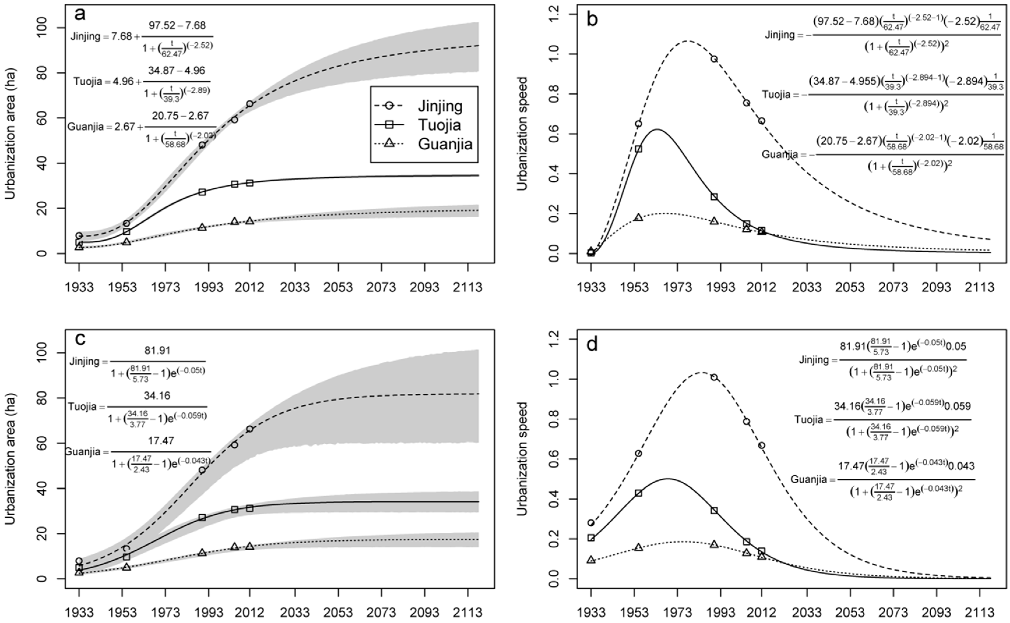
The area changes of the urban cores were fitted by 3PL and 4PL (Figure 8). As reflected by the high R2 and low RSME values (Table 2), both of the logistic models showed a good fit, while the latter model presented a slightly better fit than the former. According to the 4PL simulation, the urban core areas of Jinjing, Tuojia, and Guanjia reached their peaks in 2090, 2033, and 2050, respectively (Figure 8a). The urbanization rate differed among the three urban cores. Jinjing experienced a rapid rate of urbanization, whereas Tuojia and Guanjia underwent slower urbanization rates. The three urban cores had already passed the most rapid development stage (1970s) (Figure 8b).
3.2. Relationship between Urban Cores and Surrounding Residential Areas
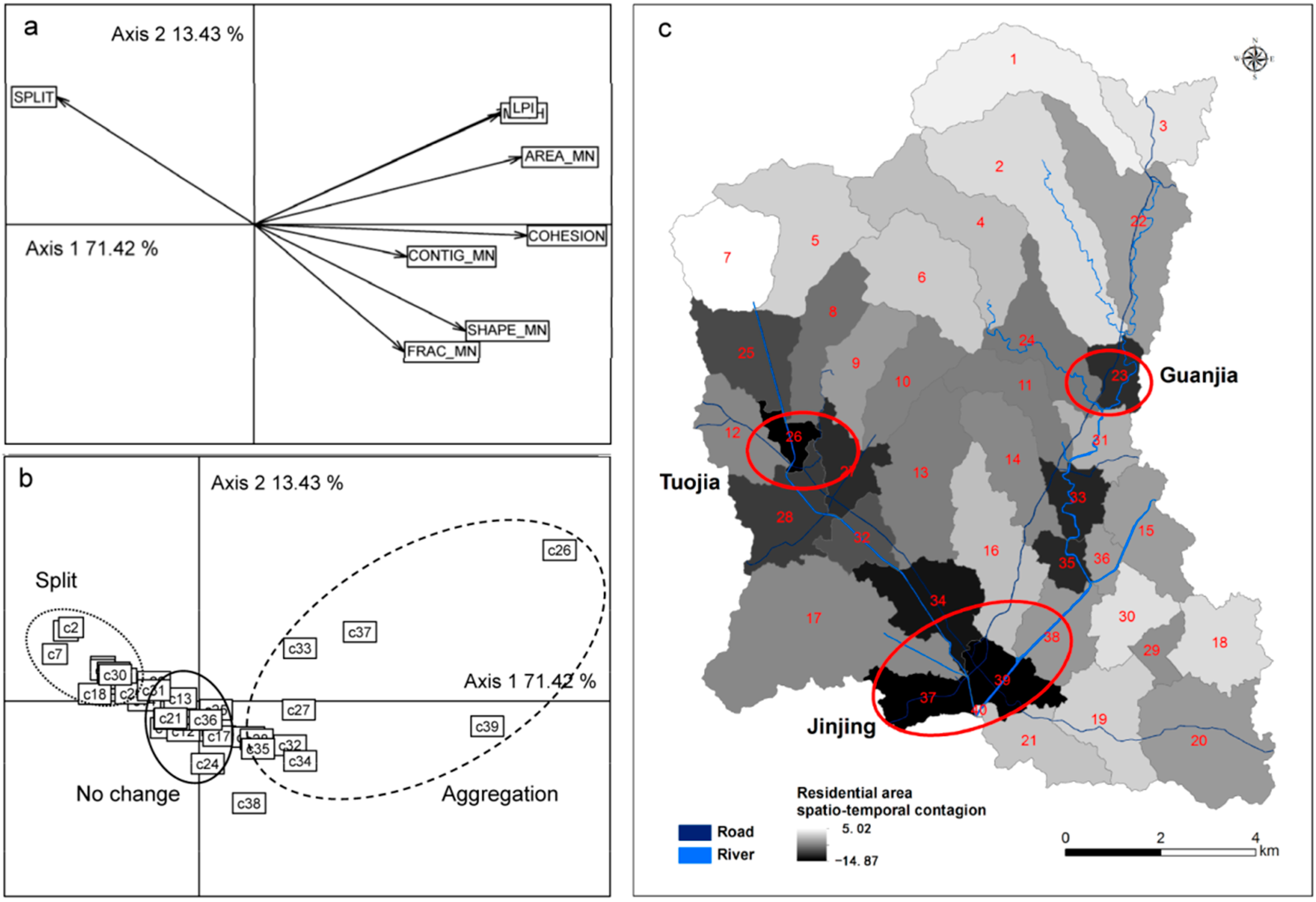
Figure 9 shows the dynamics of spatio-temporal variability of residents for the period from 1933 to 2012 in Jinjing Town. The major gradients were determined by interpreting the first two axes of the PTA (Figure 9a). Axis 1 (71.4% of the total inertia) opposed the landscape indices “LPI”, “MESH”, “AREA”, “CONTIG_MN” to “SPLIT” (Figure 9a), indicating that the first axis provided a gradient of the accumulation of residents, with the highest level of aggregation shown on the right side of the figure. Figure 9b shows the classifications of the 39 catchments. Based on the clusters of the landscape indices shown in Figure 9a, the 39 catchments were divided into three groups: Aggregated, split, and stabilized (no change) (Figure 9b). The value of each catchment was matched with the spatial attribute presented in Figure 9c. Catchments 26, 37, and 39, which contained most of the urban cores of Tuojia and Jinjing, typically aggregated, whereas Catchments 2 and 7 typically became more separated (split). The difference in residential changes in each catchment reflected population migration from Catchments 2 and 7 (the split region) to Catchments 26, 37, and 39 (urban cores).
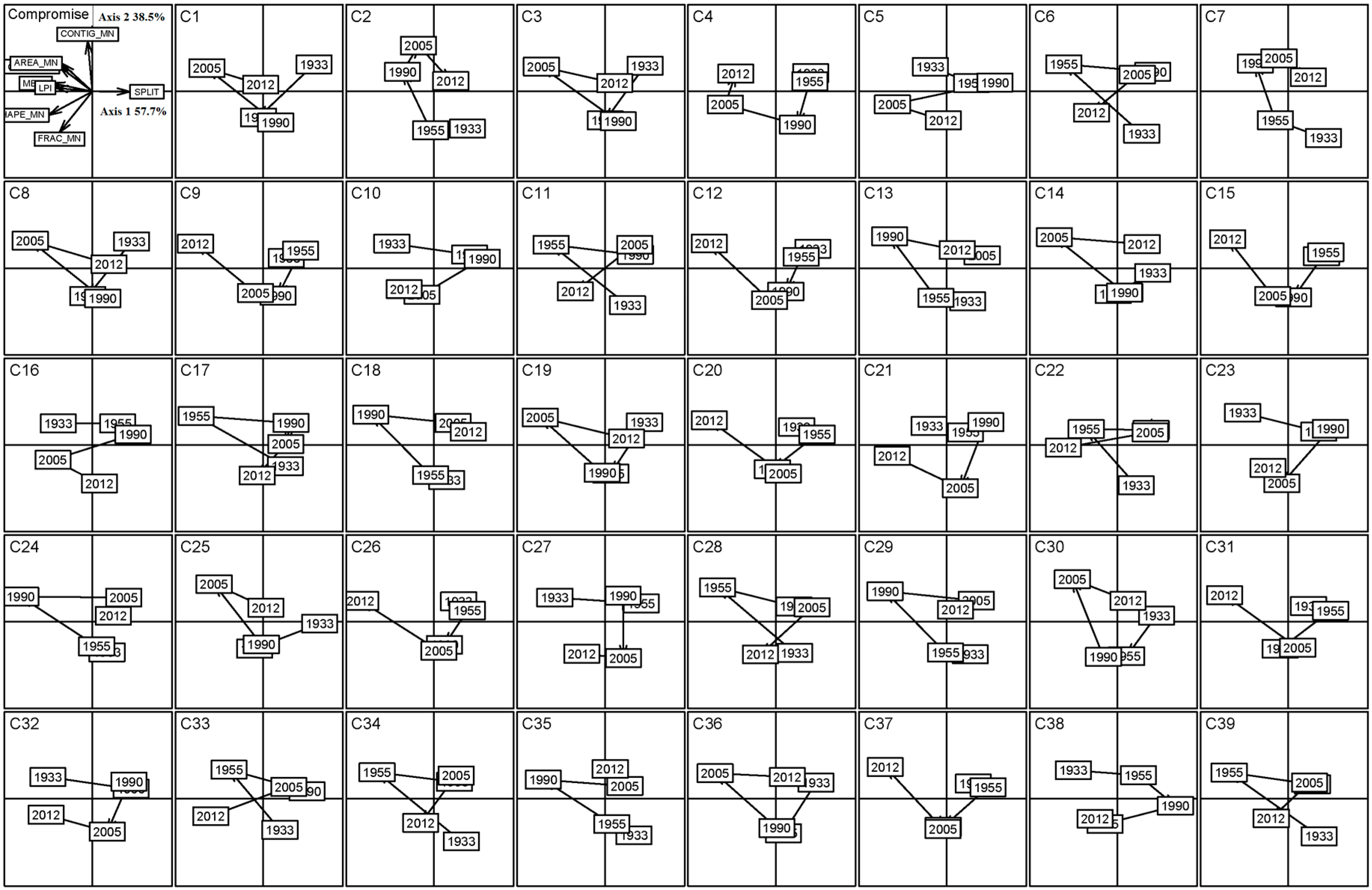
Figure 10 shows the dynamic trajectories of residential changes in each catchment for the period from 1933 to 2012. Axis 1 (57.7% of the total inertia) opposed the landscape indices “LPI”, “MESH”, “AREA” to “SPLIT”, and as in Figure 6, provided a gradient of the accumulation of residents, with the highest level of aggregation shown on the left side of the figure. The trajectories of the residential changes differed by catchment. For example, Catchments 2 and 7 (the split region) had similar historical trajectories, i.e., from splitting to aggregation and then back to splitting; Catchment 26 (Tuojia’s urban core) was consistently aggregated; and Catchments 33 and 39 (Jinjing’s urban core) changed from split to aggregated, to split, and eventually back to aggregated.
3.3. Driving Forces of the Urbanization Process
3.3.1. Population and Policies
From 1955 to 1990, the areas of urban cores and population increased at a more rapid rate than those from 1933 to 1955 (Figure 7b), indicating that the increasing population may be a major driving force for urbanization. Meanwhile, the total residential area also increased with the number of total residents across Jinjing Town. From 1990 to 2012, especially, after the implementation of township merger policy, the population stopped increasing, whereas the area of urban cores continued to increase, especially that of Jinjing’s urban cores, which increased significantly faster than those of Tuojia’s and Guanjia’s urban cores from 1990 to 2012. The results indicated that the township merger promoted urban core development in the Jinjing Town.
3.3.2. Spatial Driving Forces
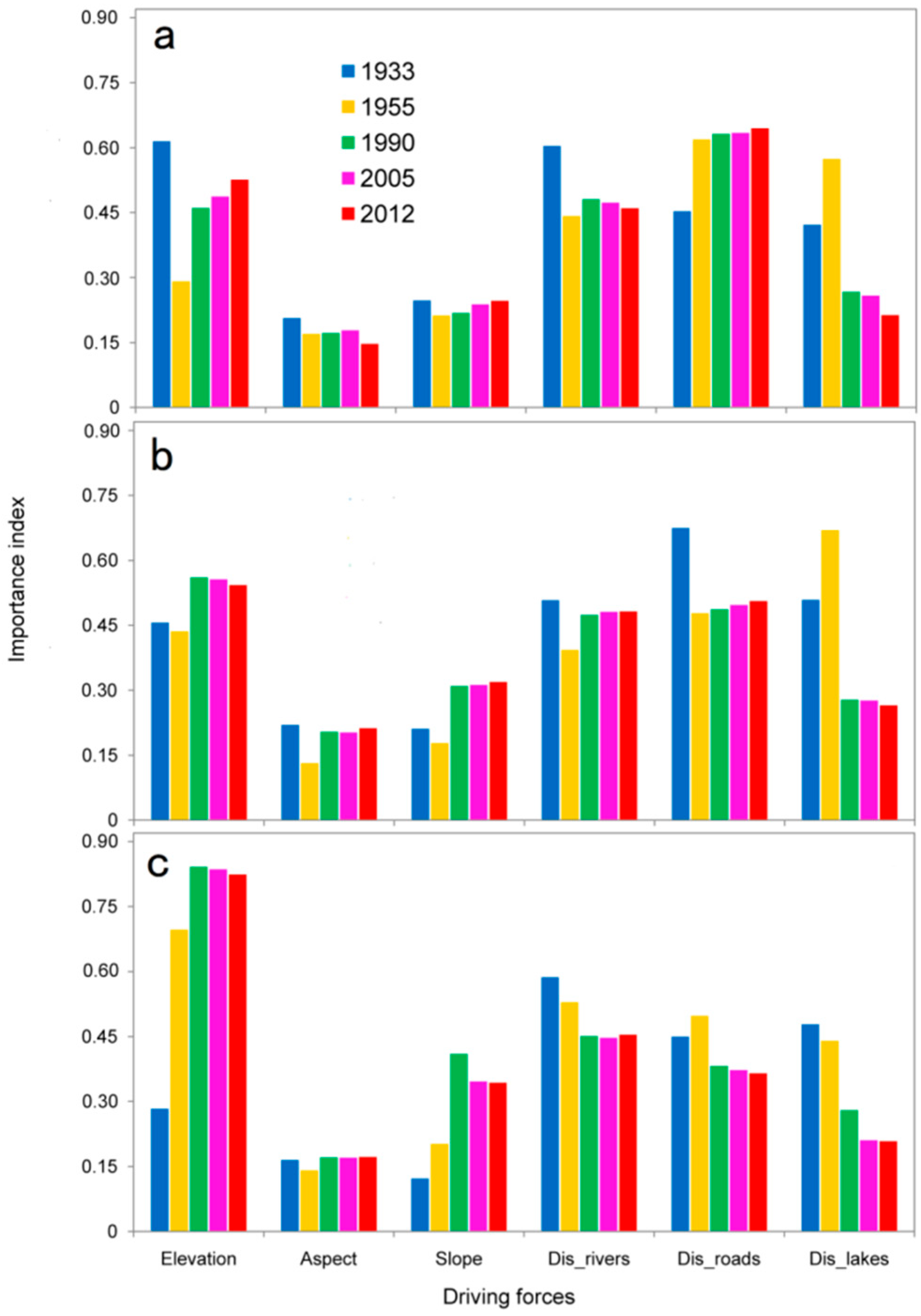
The importance of six driving forces, namely, elevation, aspect, slope, dis_rivers, dis_roads, and dis_lakes, differed for the three urban cores during the period from 1933 to 2012 (Figure 11). However, elevation and dis_roads were always predominant, indicating that these two driving forces were primary factors in shaping urban patterns in the Jinjing Town.
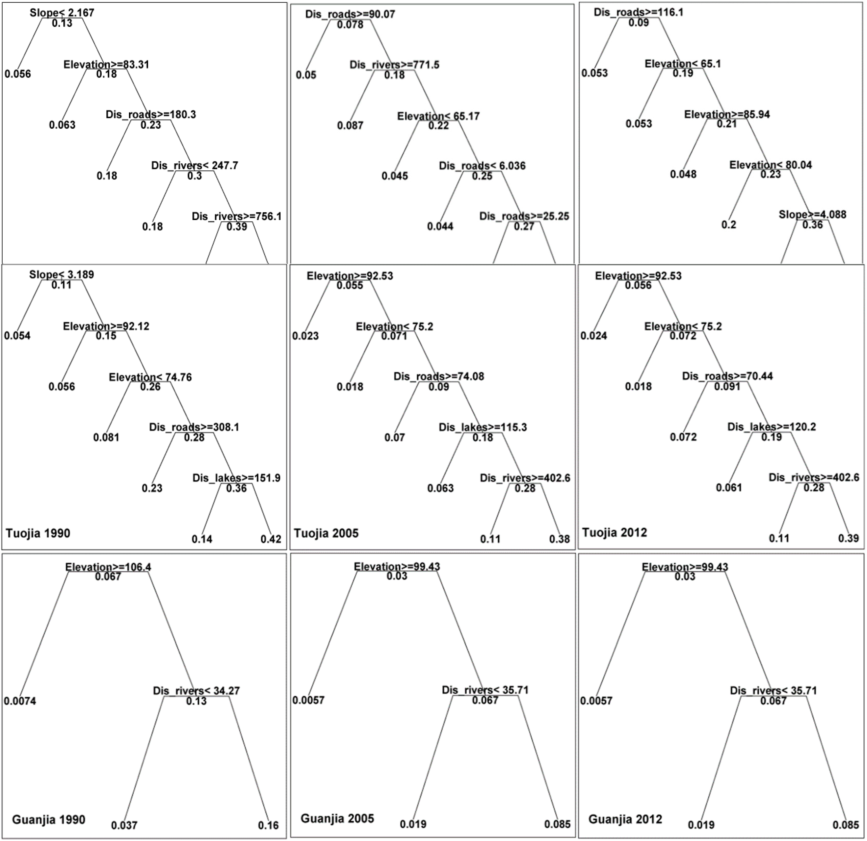
Since the examined urban cores gradually developed after 1955 in Jinjing Town (Figure 6 and Figure 7), CTA was only used to analyze the influences of the examined driving forces on urbanization processes from 1990 to 2012. In the obtained CTA model (Figure 12), the tree structures for Jinjing and Tuojia from 1990 to 2012 were more complicated than that for Guanjia. However, there were obvious differences at each layer and tree node between Jinjing and Tuojia. For example, in 2005 and 2012, the first layer of the trees was dis_roads and elevation for Jinjing and Tuojia, respectively, indicating that the most important determinants of spatial sprawl differed for these two urban cores. A comparison of the tree models for the three urban cores showed that the complexity (tree shape) did not change from 1990 to 2012, but the layers and node values of the tree model for Jinjing changed to a greater degree than those for Tuojia and Guanjia, indicating that Jinjing’ urban core experienced a more complicated development process.
4. Discussion
4.1. Urbanization Change Rates and Logistic Model Simulation
Urbanization speeds were well reflected by the areas changes of urban cores and the relatively fast and steady developing period were also successfully predicted. The areas of the urban cores replaced the share of people in the calculation of urbanization speed (Figure 5), which is in contrast to general studies of urbanization levels indicated by the share of people living in cities [34]. The main reason for this was that the majority of residents in urban cores are farmers who still own farmland, and they are merely doing business in urban cores at the town scale. Therefore, there are two types of people in urban cores: Local residents whose homesteads are in the urban areas and residents who have migrated from remote areas (hinterland) and resettled in the town and who may have more than one homestead. This phenomenon has likewise been called the double occupation of rural–urban land in China as a result of urbanization [2,35]. Consequently, accurate statistical data on the urban core populations from town governments are lacking. In contrast, population statistics are available for cities based on HuKou and temporary residence permits in China [35].
Trends in urban area change could be well fitted by the two logistic models (Table 2 and Figure 5), and 4PL performed somewhat better than 3PL. However, compared with 4PL, 3PL has been used more often to fit urbanization curves in most urbanization studies [34,36]. The parameter k in 3PL reflects the urbanization change rate, which is mostly used at a national scale, e.g., 0.0463 for China [2]. In this study, the k values were 0.050, 0.058, and 0.043 for Jinjing, Tuojia, and Guanjia, respectively. It seems that urbanization has been more rapid in Jinjing and Tuojia than in Guanjia, and in the nation as a whole. Moreover, the three urban curves show a clear S shape. This is in contrast with many other urbanization studies on urban clusters or counties, in which urban area has been found to have exponentially increased from 1978 to 2008 [4]. This discrepancy is mainly due to the difference in the study time range. For example, in this study, if we merely investigated the urban area change for the period from 1990 to 2012, the trend of urban area change would also fit to an exponential curve (Figure 5). However, given the influence of natural and socio-economical determinants of urban spatial sprawl, especially slow population growth, the urban core areas could not increase faster than during the 1970s in Jinjing Town. Considering the fitted curves for the urban area change (Figure 6), the expansion processes of these urban cores can be divided into three stages of development [34,36]. In the first stage (1933–1975), the urbanization rate was slow for all the urban cores because of the small population and certain important historical events, e.g., the Anti-Japanese War (1937–1945), China’s Liberation War (1945–1949), the Great Leap Forward (1958–1960), and the Cultural Revolution (1966–1976). In the second stage (1976–1990), each urban area experienced their fastest urbanization rate primarily because China’ urban policy focused on developing towns and small cities during 1978–1999. The period preceding the peak differed for the three urban cores. This phenomenon primarily occurred owing to the natural environments and governmental policies of the urban cores [2]. In the third stage (1991–), population grew at a sluggish rate. Population migration and the township merger promoted urban core progress in Jinjing Town. Jinjing’s urban core experienced rapid development, whereas Tuojia’s and Guanjia’s urban cores slowly developed after a period of rapid development.
4.2. Urban Core Sprawl and Residential Migration
The spatio-temporal sprawl of urban cores and their interactions with the surrounding rural residential areas were well revealed by PTA analysis, and implied that the town experienced different historically aggregating and splitting trajectories. Urban cores and surrounding residents exhibited distinct spatio-temporal dynamic characteristics that influenced each other, as revealed and quantified by the PTA (Figure 6). The areas of the urban cores obviously increased from 1933 to 2012, which is consistent with that in the urban areas at higher levels of the urban hierarchy in China [2,3,37]. However, the modes of spatio-temporal urban sprawl are distinct between towns and urban areas at higher levels of the urban hierarchy, e.g., urban clusters, provincial capital cities, and prefectural-level cities. In the literature, three modes of spatio-temporal urban sprawl (infilling, edge expansion, and leapfrogging) have been identified for urban areas at higher levels of the urban hierarchy in China, which could have substantial impacts on neighboring areas and promote the coordinated development of large, medium, and small cities, as well as small towns [3,4]. In contrast to urban areas at higher levels of the urban hierarchy, towns show only one mode of urban development, i.e., edge expansion, which is mainly due to the small scale of spatial sprawl in the urban cores of towns and the lack of comprehensive planning. From 1933 to 1990, population and residential area increases were a notable tendency in Jinjing Town, and migration from remote regions to urban cores became a major trend after 1990 (Figure 2 and Figure 6c). Enterprises in the township grew, absorbed surplus labor, and contributed to help small cities flourish. These observations are comparable to observations regarding resident changes across China [2,35]. The three urban cores experienced different historical trajectories (Figure 6). For instance, Tuojia’s urban core was consistently aggregated, and Jinjing’s urban core changed from split to aggregated, to split, and eventually back to aggregated, although all of the urban cores were more aggregated than other places in Jinjing Town. As a result, these urban cores showed different historical trajectories with respect to the surrounding residential areas and paddy fields, as shown in Figure 3 and Figure 7. In addition to agricultural land loss, the inter conversions of agricultural land types were also impacted by urbanization. For examples, paddy fields were transformed to tea fields and vegetable fields surrounding the three urban core areas in order to promote economic development (Figure 5), and several tea manufacturing companies and vegetable-production bases have been established in recent decades. Specifically, from 1990 to 2012, 102 ha of paddy fields were converted to tea fields and vegetable fields in Jinjing Town [38].
4.3. Urban Core Developments and the Driving Forces
The key drivers (township merger, elevation and distance to roads, and population migration) were identified in the spatial sprawl of urban cores, indicating that CTA and RF are efficient for quantifying the mechanism of urban core spatial sprawl and the importance of each driving force. The main reason is that among the ensemble-based classifiers, CTA and RF classifiers are efficient for input predictors with a different nature, and insensitive to noise, outliers, and overtraining. Moreover, they are computationally much faster than boosting-based ensemble methods and somewhat faster than simply bagging [33]. Moreover, determining and collecting data on the driving forces of urbanization is more difficult for towns than for urban areas at higher levels of the urban hierarchy, primarily because of the difficulty of obtaining high resolution spatial data and the lack of authoritative socio-economic data [10]. In this study, the influences of population changes, urban development policies, and spatial driving forces were analyzed over different periods. However, an adequate analysis of economic driving forces of urbanization could not be performed for the following three reasons: Firstly, township officials are the lowest ranked officials in China’s government hierarchy and, therefore, very few government responsibilities have been defined, except for those of the Birth Planning Commission [35]; secondly, the methods for collecting economic statistics and the units of the data have differed over various historical periods [2]. Thus, it was difficult to standardize and compare these economic data for a period covering over more than 80 years, from 1933 to 2012; and thirdly, in contrast to large cities, the examined urban cores showed no obvious differences with respect to the three major traditional industries that generally reflect economic development. Specifically, the urban cores were dominated by commodity trading business and agriculture-based manufacturing industries, e.g., tea and food processing, which serve both surrounding villages and large cities [2]. The increments of urban core areas were mainly associated with socio-economic factors, such as population change and urban development policy. In addition, spatial distribution factors, e.g., DEM or distance to roads and rivers, played prominent roles at the town scale (Figure 8 and Figure 9). The differences in the determinants of urbanization could be reflected in the modes of urban cores expansion. For example, Jinjing and Tuojia developed in clusters and along roads for convenient transportation, in line with the development in most cities [2,3], whereas Guanjia showed a more dispersed development owing to the impact of elevation. The analysis of the determinant’s importance aimed not only to aid urban development planning but also to evaluate future changes in the urban areas by calculating probability maps [12,15].
5. Conclusions
In this study, a comprehensive framework was established for modeling urban spatial dynamics based on multidisciplinary theories, e.g., landscape ecology, urban function development, and land-use change modeling theory. Some traditional methods, such as landscape indices for examining spatial pattern changes in the urban core area and urbanization curves for quantifying urbanization levels, were developed for urbanization research at the town scale. Besides, partial triadic analysis, as a powerful three-dimensional spatio-temporal method, was introduced to explore the spatio-temporal urbanization process and relationships between urban cores and surrounding settlements. Moreover, other methods, e.g., classification tree analysis and random forest analysis, were used to analyze the driving forces of spatial sprawl of urban cores. By using the comprehensive framework, Jinjing Town was chosen to research the spatio-temporal process of urbanization at the town scale. These results suggest that a comprehensive approach is powerful for quantifying the spatio-temporal growth of urban cores at the township level. Jinjing Town typifies many towns in terms of geo-morphology and socio-economic dynamics, but before we are able to apply the comprehensive approach to address urban developing issues at the practice level, further research at other places is needed, for instance, whether or not the rate, mode, driving forces, and research methodologies of urban core development at the town scale are obviously different from those at other levels of the urban hierarchy in China.
Author Contributions
Conceptualization, X.L. and Y.W.; methodology, X.L., Y.L. and Y.W.; validation, X.L., Y.L., J.W. and Y.W.; formal analysis, X.L.; investigation, X.L. and Y.W.; resources, X.L. and Y.W.; writing—original draft preparation, X.L.; writing—review and editing, X.L. and Y.W.
Funding
This research was funded by the National Key Research and Development Program of China (2017YFD0800105), the National Natural Science Foundation of China (41301202), Youth Innovation Team Project of ISA, CAS (2017QNCXTD_LF), and Young Scientists Fund of the National Natural Science Foundation of China (31401943).
Conflicts of Interest
The authors declare no conflict of interest.
References
- Xiang, W.N.; Stuber, R.M.B.; Meng, X. Meeting critical challenges and striving for urban sustainability in China. Landsc. Urban Plan. 2011, 100, 418–420. [Google Scholar] [CrossRef]
- Gu, C.L.; Wu, L.Y.; Cook, I. Progress in research on Chinese urbanization. Front. Archit. Res. 2012, 1, 101–149. [Google Scholar] [Green Version]
- Wu, J.G.; Xiang, W.N.; Zhao, J.Z. Urban ecology in China: Historical developments and future directions. Landsc. Urban Plan. 2014, 125, 222–233. [Google Scholar] [CrossRef]
- Li, C.; Li, J.X.; Wu, J.G. Quantifying the speed, growth modes, and landscape pattern changes of urbanization: A hierarchical patch dynamics approach. Landsc. Ecol. 2013, 28, 1875–1888. [Google Scholar] [CrossRef]
- Jim, C.Y.; Chen, S.S. Comprehensive greenspace planning based on landscape ecology principles in compact Nanjing city, China. Landsc. Urban Plan. 2003, 65, 95–116. [Google Scholar] [CrossRef]
- Nassauer, J.I.; Wu, J.G.; Xiang, W.N. Actionable urban ecology in China and the world: Integrating ecology and planning for sustainable cities. Landsc. Urban Plan. 2014, 125, 207–208. [Google Scholar] [CrossRef]
- Xu, Y.; Tang, Q.; Fan, J.; Bennett, S.J.; Li, Y. Assessing construction land potential and its spatial pattern in China. Landsc. Urban Plan. 2011, 103, 207–216. [Google Scholar] [CrossRef]
- Liu, X.L.; Wang, Y.; Li, Y.; Liu, F.; Shen, J.L.; Wang, J.; Xiao, R.L.; Wu, J.S. Changes in arable land in response to township urbanization in a Chinese low hilly region: Scale effects and spatial interactions. Appl. Geogr. 2017, 88, 24–37. [Google Scholar] [CrossRef]
- Fang, C.L. The urbanization and urban development in China after the reform and opening-up. Econ. Geogr. 2009, 29, 19–25. [Google Scholar]
- Cohen, B. Urban growth in developing countries: A review of current trends and a caution regarding existing forecasts. World Dev. 2004, 32, 23–51. [Google Scholar] [CrossRef]
- Deng, X.Z.; Bai, X.M. Sustainable urbanization in Western China. Environ. Sci. Policy Sustain. Dev. 2014, 56, 12–24. [Google Scholar] [CrossRef]
- Tan, M.H.; Li, X.B. The changing settlements in rural areas under urban pressure in China: Patterns, driving forces and policy implications. Landsc. Urban Plan. 2013, 120, 170–177. [Google Scholar] [CrossRef]
- Su, S.L.; Ma, X.Y.; Xiao, R. Agricultural landscape pattern changes in response to urbanization at ecoregional scale. Ecol. Indic. 2014, 40, 10–18. [Google Scholar] [CrossRef]
- Chen, Y.G. Urban chaos and perplexing dynamics of urbanization. Lett. Spat. Resour. Sci. 2009, 2, 85–95. [Google Scholar] [CrossRef]
- Irwin, E.G.; Jayaprakash, C.; Munroe, D.K. Towards a comprehensive framework for modeling urban spatial dynamics. Landsc. Ecol. 2009, 24, 1223–1236. [Google Scholar] [CrossRef]
- Haregeweyn, N.; Fikadu, G.; Tsunekawa, A.; Tsubo, M.; Meshesha, D.T. The dynamics of urban expansion and its impacts on land use/land cover change and small-scale farmers living near the urban fringe: A case study of Bahir Dar, Ethiopia. Landsc. Urban Plan. 2012, 106, 149–157. [Google Scholar] [CrossRef]
- Hsieh, S.-C. Analyzing urbanization data using rural–urban interaction model and logistic growth model. Comput. Environ. Urban Syst. 2014, 45, 89–100. [Google Scholar] [CrossRef]
- Liu, X.P.; Li, X.; Chen, Y.M.; Tan, Z.Z.; Li, S.Y.; Ai, B. A new landscape index for quantifying urban expansion using multi-temporal remotely sensed data. Landsc. Ecol. 2010, 25, 671–682. [Google Scholar] [CrossRef]
- Aguilera, F.; Valenzuela, L.M.; Botequilha-Leitão, A. Landscape metrics in the analysis of urban land use patterns: A case study in a Spanish metropolitan area. Landsc. Urban Plan. 2011, 99, 226–238. [Google Scholar] [CrossRef]
- Mitsova, D.; Shuster, W.; Wang, X. A cellular automata model of land cover change to integrate urban growth with open space conservation. Landsc. Urban Plan. 2011, 99, 141–153. [Google Scholar] [CrossRef]
- Cheng, J.; Masser, I. Urban growth pattern modeling: A case study of Wuhan city, PR China. Landsc. Urban Plan. 2003, 62, 199–217. [Google Scholar] [CrossRef]
- Muriuki, G.; Seabrook, L.; McAlpine, C.; Jacobson, C.; Price, B.; Baxter, G. Land cover change under unplanned human settlements: A study of the Chyulu Hills squatters, Kenya. Landsc. Urban Plan. 2011, 99, 154–165. [Google Scholar] [CrossRef]
- Gu, S.Z.; Zheng, L.Y.; Yi, S. Problems of Rural migrant workers and policies in the New period of urbanization. Chin. J. Popul. Resour. Environ. 2008, 6, 14–20. [Google Scholar] [CrossRef]
- Tayyebi, A.; Perry, P.C.; Tayyebi, A.H. Predicting the expansion of an urban boundary using spatial logistic regression and hybrid raster–vector routines with remote sensing and GIS. Int. J. Geogr. Inf. Sci. 2014, 28, 639–659. [Google Scholar] [CrossRef]
- Pijanowski, B.C.; Tayyebi, A.; Doucette, J.; Pekin, B.K.; Braun, D.; Plourde, J. A big data urban growth simulation at a national scale: Configuring the GIS and neural network based Land transformation model to run in a high performance computing (HPC) environment. Environ. Model. Softw. 2014, 51, 250–268. [Google Scholar] [CrossRef]
- Andersson, E.; Ahrné, K.; Pyykönen, M.; Elmqvist, T. Patterns and scale relations among urbanization measures in Stockholm, Sweden. Landsc. Ecol. 2009, 24, 1331–1339. [Google Scholar] [CrossRef] [Green Version]
- R Development Core Team R: A Language and Environment for Statistical Computing. Available online: http://www.R-project.org/ (accessed on 5 July 2019).
- Chessel, D.; Dufour, A.B.; Thioulouse, J. The ade4 package-I: One-table methods. R News 2004, 4, 5–10. [Google Scholar]
- Dray, S.; Dufour, A.B.; Chessel, D. The ade4 package-II: Two-table and K-table methods. R News 2007, 7, 47–52. [Google Scholar]
- Liaw, A.; Wiener, M. Classification and regression by random Forest. R News 2002, 2, 18–22. [Google Scholar]
- Therneau, T.; Atkinson, B.; Ripley, B. Rpart: Recursive partitioning and regression trees. R package version 4. 2015, pp. 1–9. Available online: http://CRAN.R-project.org/package=rpart (accessed on 29 June 2015).
- Hamann, A.; Gylander, T.; Chen, P.Y. Developing seed zones and transfer guidelines with multivariate regression trees. Tree Genet. Genomes 2011, 7, 399–408. [Google Scholar] [CrossRef]
- Breiman, L. Random forests. Mach. Learn. 2001, 45, 5–32. [Google Scholar] [CrossRef]
- Mulligan, G.F. Revisiting the urbanization curve. Cities 2013, 32, 113–122. [Google Scholar] [CrossRef]
- Chan, K.W. The Chinese Hukou system at 50. Eurasian Geogr. Econ. 2009, 50, 197–221. [Google Scholar] [CrossRef]
- Chen, M.; Ye, C.; Zhou, Y. Comments on Mulligan’s “Revisiting the urbanization curve”. Cities 2014, 41, 54–56. [Google Scholar] [CrossRef]
- Ye, J.A.; Xu, J.; Yi, H. The fourth wave of urbanization in China. City Plan. Rev. 2006, 30, 13–18. [Google Scholar]
- Liu, X.L.; Li, Y.; Shen, J.L.; Fu, X.Q.; Xiao, R.L.; Wu, J.S. Landscape pattern changes at a catchment scale: A case study in the upper Jinjing river catchment in subtropical central China from 1933 to 2005. Landsc. Ecol. Eng. 2014, 10, 263–276. [Google Scholar] [CrossRef]
Figure 1.
Methodological flow chart.

Figure 2.
Tridimensional table of data. (A) Identification of a spatial structure common to the 5 dates and study of this temporal permanence. (B) Identification of a temporal structure common to the 39 sub-catchments and study of this spatial permanence.
Figure 2.
Tridimensional table of data. (A) Identification of a spatial structure common to the 5 dates and study of this temporal permanence. (B) Identification of a temporal structure common to the 39 sub-catchments and study of this spatial permanence.

Figure 3.
Flowchart showing the procedures for data acquisition and processing.

Figure 4.
Geographical location of Jinjing Town, located in the north of Changsha County in the Changsha–Zhuzhou–Xiangtan urban cluster, Hunan province, China. Jinjing Town was divided into 39 catchments, with elevations between 56 and 440 m.
Figure 4.
Geographical location of Jinjing Town, located in the north of Changsha County in the Changsha–Zhuzhou–Xiangtan urban cluster, Hunan province, China. Jinjing Town was divided into 39 catchments, with elevations between 56 and 440 m.

Figure 5.
Spatial distribution of residential areas in Jinjing Town from 1933 to 2012.

Figure 6.
Spatio-temporal patterns of the three urban cores (Jinjing, Tuojia, and Guanjia) from 1933 to 2012.
Figure 6.
Spatio-temporal patterns of the three urban cores (Jinjing, Tuojia, and Guanjia) from 1933 to 2012.

Figure 7.
(a) Area changesof the urban cores (Jinjing, Tuojia, and Guanjia) and total residential area from 1933 to 2012, and (b) population changes of towns (Jinjing, Tuojia, and Guanjia) from 1933 to 2012.
Figure 7.
(a) Area changesof the urban cores (Jinjing, Tuojia, and Guanjia) and total residential area from 1933 to 2012, and (b) population changes of towns (Jinjing, Tuojia, and Guanjia) from 1933 to 2012.

Figure 8.
Simulation results of (a,b) the four-parameter logistic equation and (c,d) three-parameter logistic equation for urban core area and change ratios, respectively.
Figure 8.
Simulation results of (a,b) the four-parameter logistic equation and (c,d) three-parameter logistic equation for urban core area and change ratios, respectively.

Figure 9.
Results of the partial triadic analysis of changes in the spatio-temporal patterns for residential areas. (a) Landscape indices in Plan 1–2 of the compromise. (b) Catchments in Plan 1–2 of the compromise. (c) Spatio-temporal aggregation for residential areas in Jinjing Town, where the values were extracted from (b). AREA_MN: Patch area mean; COHESION: Patch cohesion index; CONTIG_MN: Contiguity index mean; FRAC_MN: Fractal dimension index mean; LPI: Largest patch index; MESH: Effective mesh size; SHAPE_MN: Shape index mean; and SPLIT: Splitting index. Details for the above landscape indices are shown in Table 1.

Figure 10.
Variability of the landscape dynamics at the catchment scale.

Figure 11.
Driving forces importance of spatial sprawl for the urban cores of (a) Jinjing, (b) Tuojia, and (c) Guanjia calculated by Random Forest analysis from 1933 to 2012.
Figure 11.
Driving forces importance of spatial sprawl for the urban cores of (a) Jinjing, (b) Tuojia, and (c) Guanjia calculated by Random Forest analysis from 1933 to 2012.

Figure 12.
Classification and regression tree models that describe the relationships between spatial driving forces and spatial sprawl for the three urban cores from 1990 to 2012.
Figure 12.
Classification and regression tree models that describe the relationships between spatial driving forces and spatial sprawl for the three urban cores from 1990 to 2012.


Table 1.
Description of landscape indices used in the partial triadic analysis.
| Acronym | Name | Formula | Description | Unit | Range |
|---|---|---|---|---|---|
| AREA_MN | Patch area_mean | AREA_MN = ai = area of patch i (m2); and n = total patch number | AREA_MN expresses the mean area of patches within the entire reference unit, reflecting the landscape fragmentation | Hectares | AREA_MN > 0 |
| COHESION | Patch cohesion index | COHESION = = perimeter of patch i; ai = area of path i; A = total number of cells in the landscape | COHESION measures the physical connectedness of the corresponding patch type | Dimensionless | 0 ≤ COHESION ≤ 100 |
| CONTIG_MN | Contiguity index_mean | CONTIG_MN = ni = the number of elements of the group i; G = the number of groups; dAA, dA1A1 and dAA1 = the average distances between the points belonging to group A and its complements | CONTIG_MN assesses the spatial connectedness of cells within a grid-cell patch to provide an index of the patch boundary configuration and thus patch shape | Dimensionless | 0 ≤ CONTIG_MN ≤ 1 |
| FRAC_MN | Fractal dimension index_MN | FRAC_MN = ai = area of patch i (m2); pj = perimeter of patch i (m); ni = number of patches in the landscape of patch type i | FRAC_MN describes the power relationship between the patch area and perimeter, reflecting the landscape heterogeneity. | Dimensionless | 1 ≤ FRAC_MN ≤ 2 |
| LPI | Largest patch index | LPI = ai = area of patch i (m2); A = total landscape area (m2) | Percentage of the landscape within the largest patch; identifies the dominating landscape types | Percentage | 0 < LPI ≤ 100 |
| MESH | Effective mesh size | MESH = ai = area of patch i (m2); A = total landscape area (m2) | MESH is based on the cumulative patch area distribution and is interpreted as the size of the patches | Hectares | Ratio of cell size to landscape area ≤ MESH ≤ total landscape area (A) |
| SHAPE_MN | Shape index_mean | SHAPE_MN = pi = perimeter of patch i (m); ai = area of patch i (m2) | Shape equals the patch perimeter divided by the square root of the patch area, adjusted by a constant to adjust for a square standard | Dimensionless | SHAPE_MN ≤ 1 |
| SPLIT | Splitting index | SPLIT = ai = area of patch i (m2); A = total landscape area (m2) | Split is based on the cumulative patch area distribution and is interpreted as the effective mesh number | Dimensionless | 1 ≤ SPLIT ≤ number of cells in the landscape area squared |
Table 2.
Parameters and evaluation indicators of the logistic models.
| Urban Cores | x0 | xm | t2 | k | RMSE | R2 |
|---|---|---|---|---|---|---|
| 4PL | ||||||
| Jinjing | 7.72 | 97.52 | 62.13 | 2.52 | 0.79 | 0.99 |
| Tuojia | 4.96 | 34.87 | 39.30 | 2.89 | 0.14 | 1.00 |
| Guanjia | 2.67 | 20.75 | 58.67 | 2.02 | 0.22 | 1.00 |
| 3PL | ||||||
| Jinjing | 5.73 | 81.90 | - | 0.050 | 1.58 | 0.95 |
| Tuojia | 3.77 | 34.15 | - | 0.058 | 0.26 | 0.96 |
| Guanjia | 2.43 | 17.47 | - | 0.043 | 0.76 | 0.98 |
4PL is a four-parameters logistic equation, and 3PL is a three-parameters logistic equation. The xm is the maximum area of the urban core (top of the curve); x0 is the minimum area of the urban core (bottom of the curve); t2 is the t value for the 4PL fitting curve point that is midway between the xm and x0 parameters; and k is the slope of the curve at its midpoint. The RMSE is the root mean square error.
© 2019 by the authors. Licensee MDPI, Basel, Switzerland. This article is an open access article distributed under the terms and conditions of the Creative Commons Attribution (CC BY) license (http://creativecommons.org/licenses/by/4.0/).
Share and Cite
MDPI and ACS Style
Liu, X.; Wang, Y.; Li, Y.; Wu, J. Quantifying the Spatio-Temporal Process of Township Urbanization: A Large-Scale Data-Driven Approach. ISPRS Int. J. Geo-Inf. 2019, 8, 389. https://doi.org/10.3390/ijgi8090389
AMA Style
Liu X, Wang Y, Li Y, Wu J. Quantifying the Spatio-Temporal Process of Township Urbanization: A Large-Scale Data-Driven Approach. ISPRS International Journal of Geo-Information. 2019; 8(9):389. https://doi.org/10.3390/ijgi8090389
Chicago/Turabian StyleLiu, Xinliang, Yi Wang, Yong Li, and Jinshui Wu. 2019. "Quantifying the Spatio-Temporal Process of Township Urbanization: A Large-Scale Data-Driven Approach" ISPRS International Journal of Geo-Information 8, no. 9: 389. https://doi.org/10.3390/ijgi8090389
Note that from the first issue of 2016, this journal uses article numbers instead of page numbers. See further details here.