
Uncertainty-Based Map Matching: The Space-Time Prism and k-Shortest Path Algorithm


Abstract
:1. Introduction
Organization
2. An Overview of Existing Approaches to Map Matching
2.1. Classification of Map Matching Algorithms
2.2. A Brief Review of Map Matching Algorithms
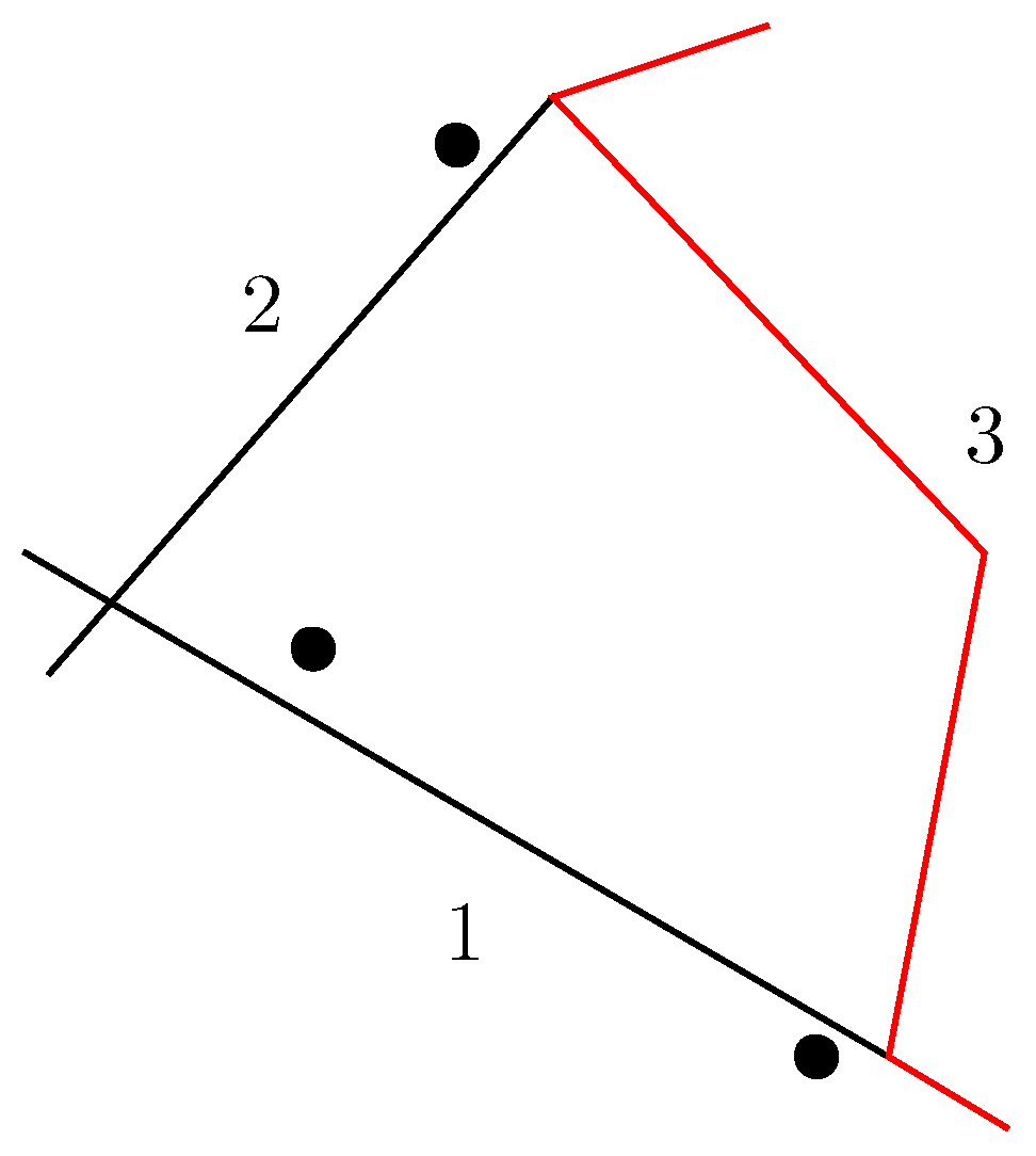
2.2.1. Geometric Algorithms
2.2.2. Topological Algorithms
2.2.3. Probabilistic Algorithms
2.3. Algorithms for Data with a Low Sampling Rate
3. An Uncertainty-Based Map Matching Algorithm
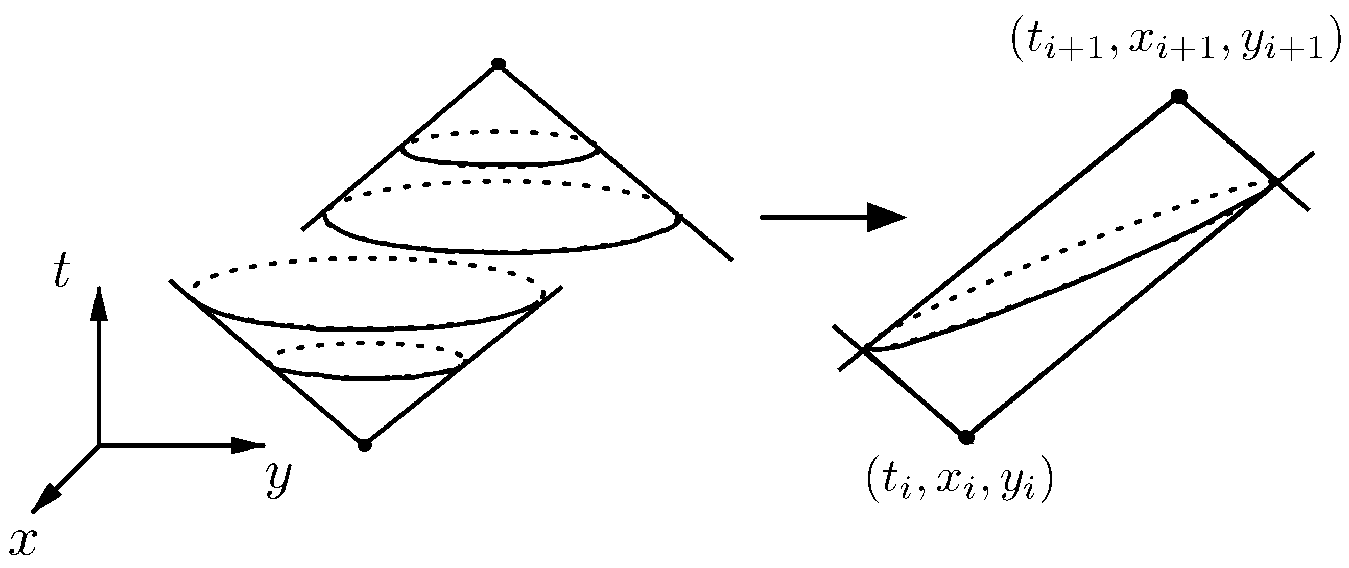
3.1. Introduction to Space-Time Prisms
3.2. Using Space-Time Prisms for Map Matching
3.2.1. Computation of the Projection of a Space-Time Prism and Its Bounding Box
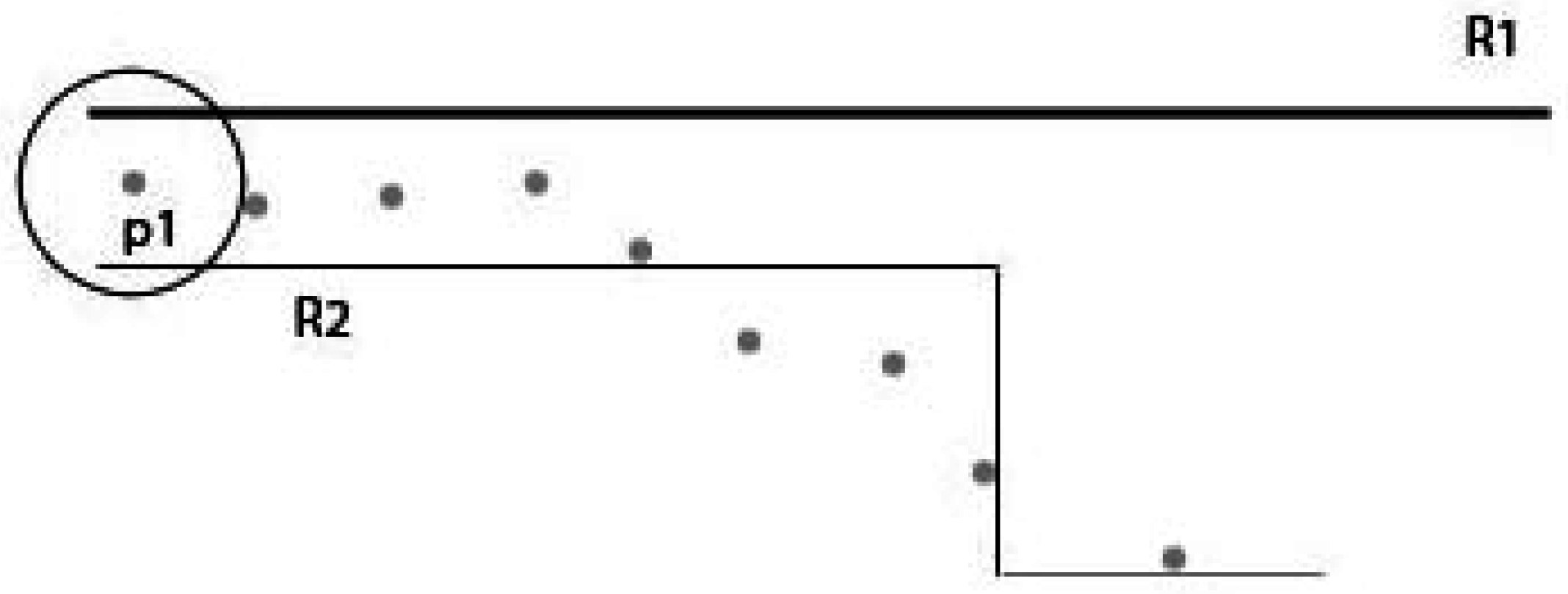
3.2.2. Using Bounding Boxes of the Projection of the Space-Time Prisms in Map Matching
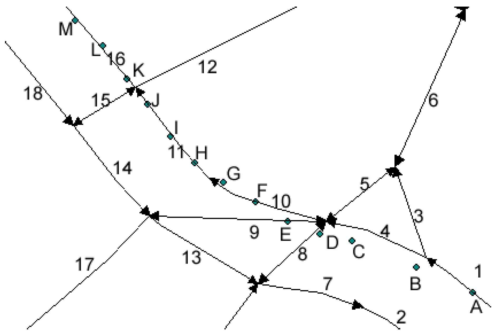
3.2.3. An Algorithm for k-Shortest Path Routing
3.2.4. Description of the Space-Time Prisms Map Matching Algorithm
- Step 1.
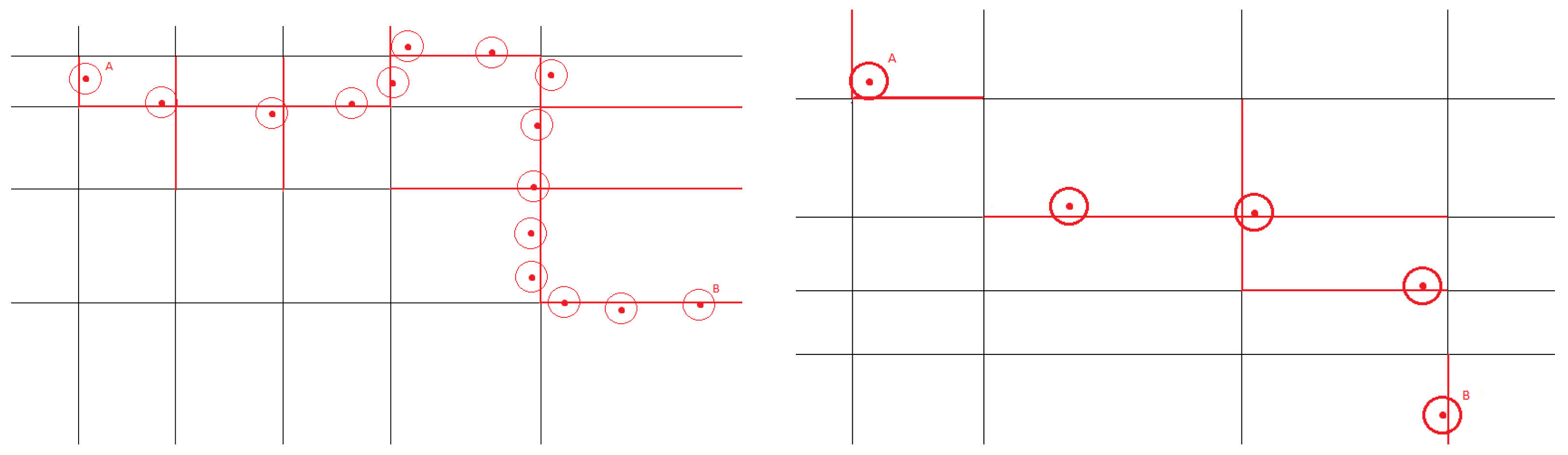
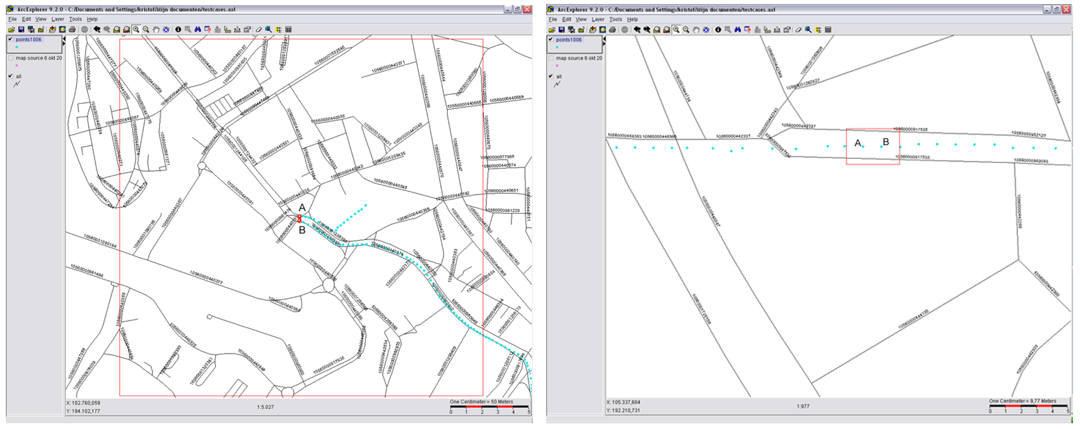
- Select the relevant parts of the road network by calculating, for each pair of consecutive points, which road segments the MO could have driven on (using the bounding boxes of the projections of space-time prisms, as described in Section 3.2).
- Step 2.
- For each sample point, compute the closest road segment, as described in Section 3.2.4, and assign scores to each road segment. A score for a segment s is computed adding up the weights of all of the segments that match s.
- Step 3.
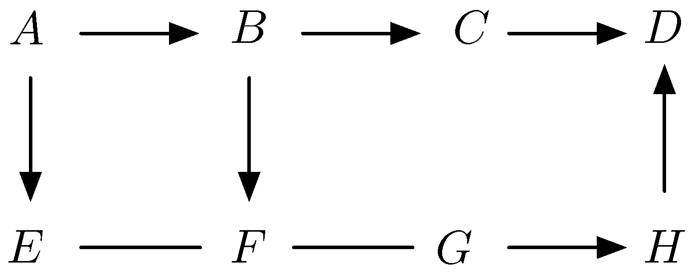
- Compute, within the limited road network determined in Step 1, the k-shortest paths, and select, as output, the shortest path with the maximum total weight. If we obtain two paths with the same weight, the first path would be selected.
4. An Improved Evaluation of Map Matching Algorithms
4.1. Data Sources and Properties
4.2. Methods to Measure the Quality of a Map Matching Algorithm
4.3. Problems in Measuring Accuracy
4.4. A New Accuracy Measure: CL-Accuracy
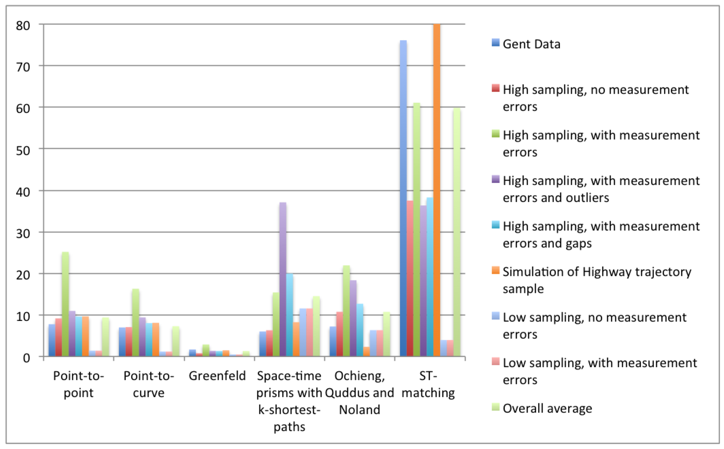
5. Experimental Comparison of Map Matching Algorithms
5.1. Tests on Human Labeled Data
5.2. Tests on Computer-Generated Data
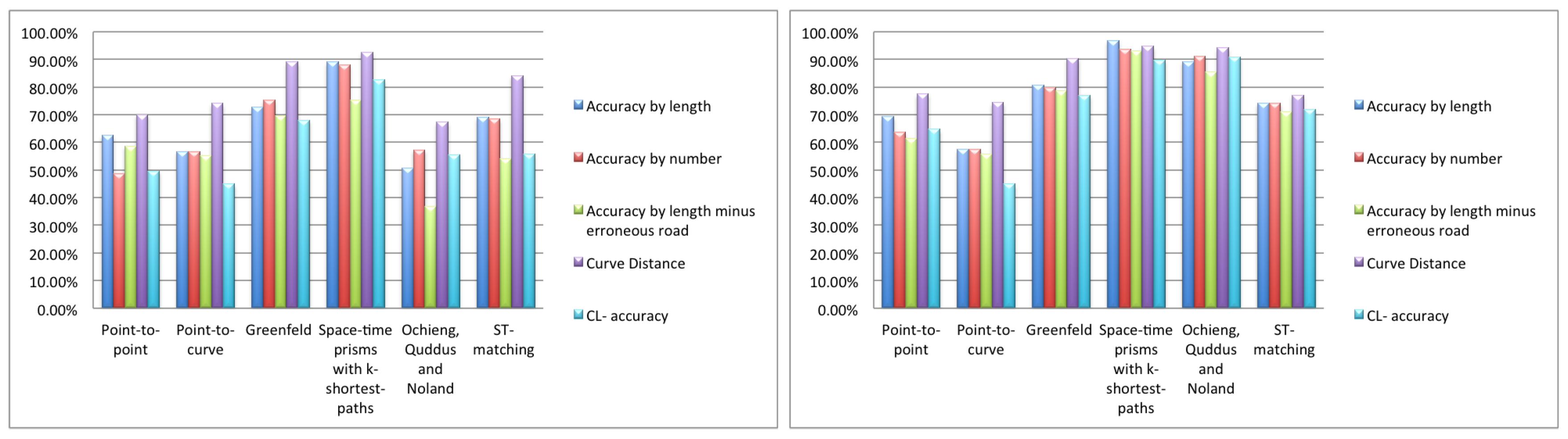
5.2.1. High Sampling Rate
Simulated Trajectory Samples with No Measurement Errors
Simulated Trajectory Samples with Measurement Errors
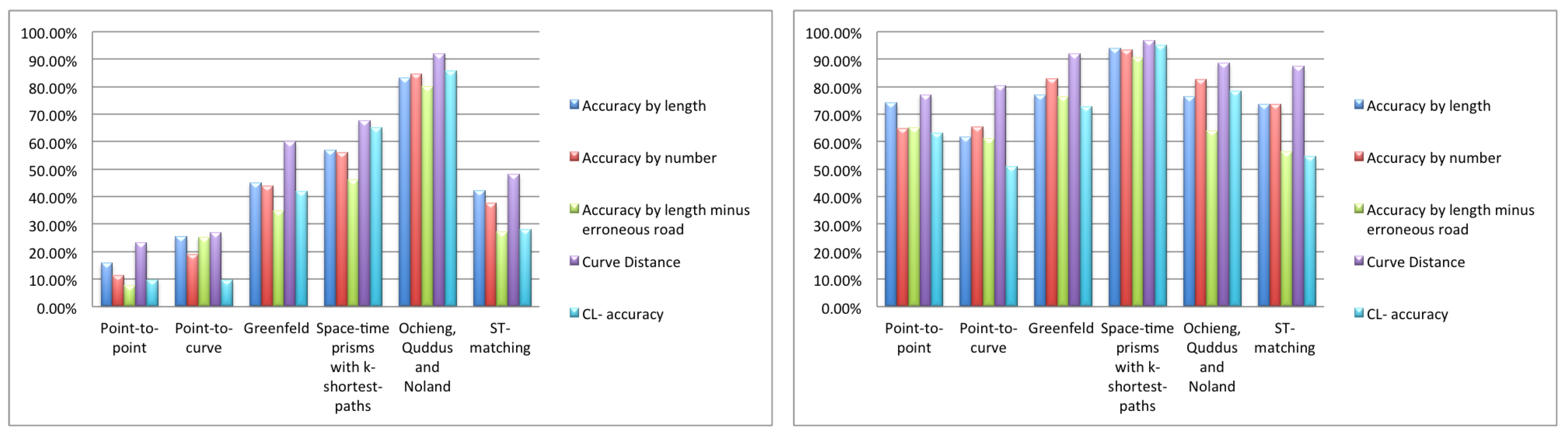
Simulated Trajectory Samples with Measurement Errors and Outliers
Simulated Trajectory Samples with Measurement Errors and Gaps
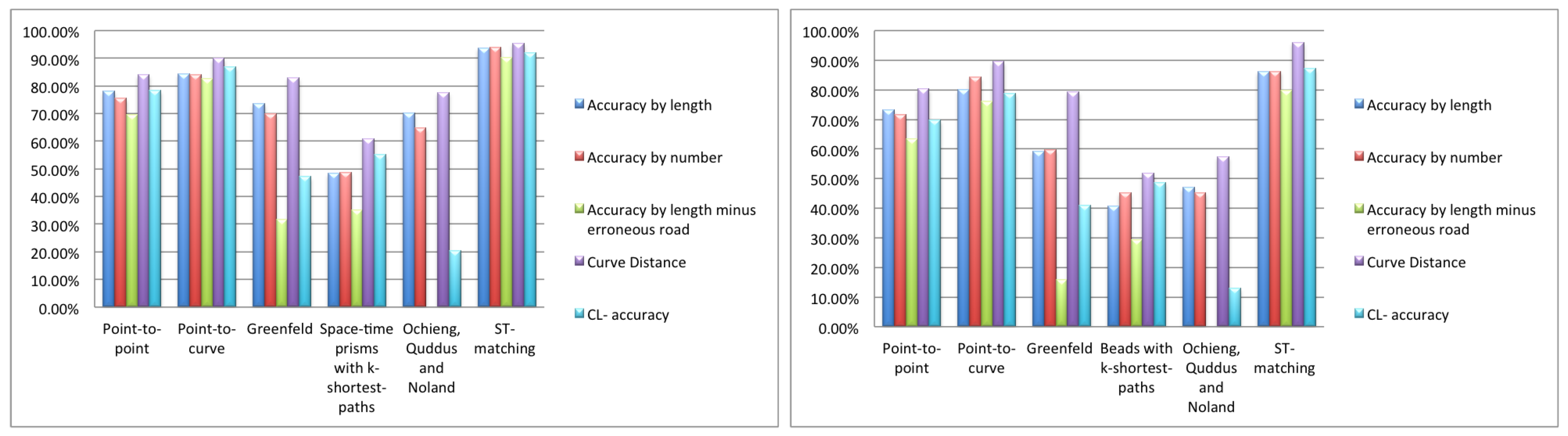
Simulated Trajectory Samples on a Highway with GPS Errors
Simulated Trajectory Samples on a Long Distance with Measurement Errors
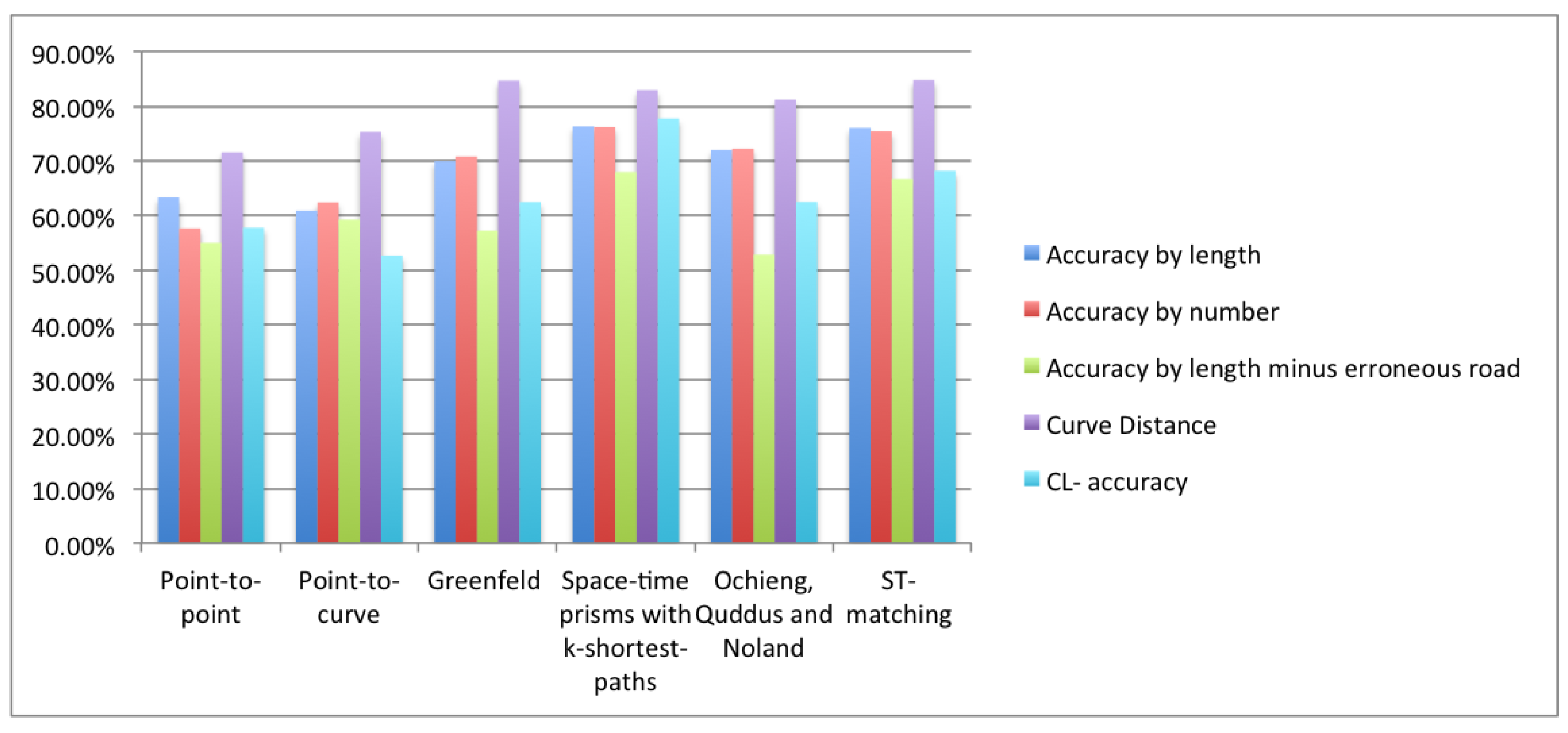
5.2.2. Low Sampling Rate
Simulated Trajectory Samples with No Measurement Errors
Simulated Trajectory Samples with Measurement Errors
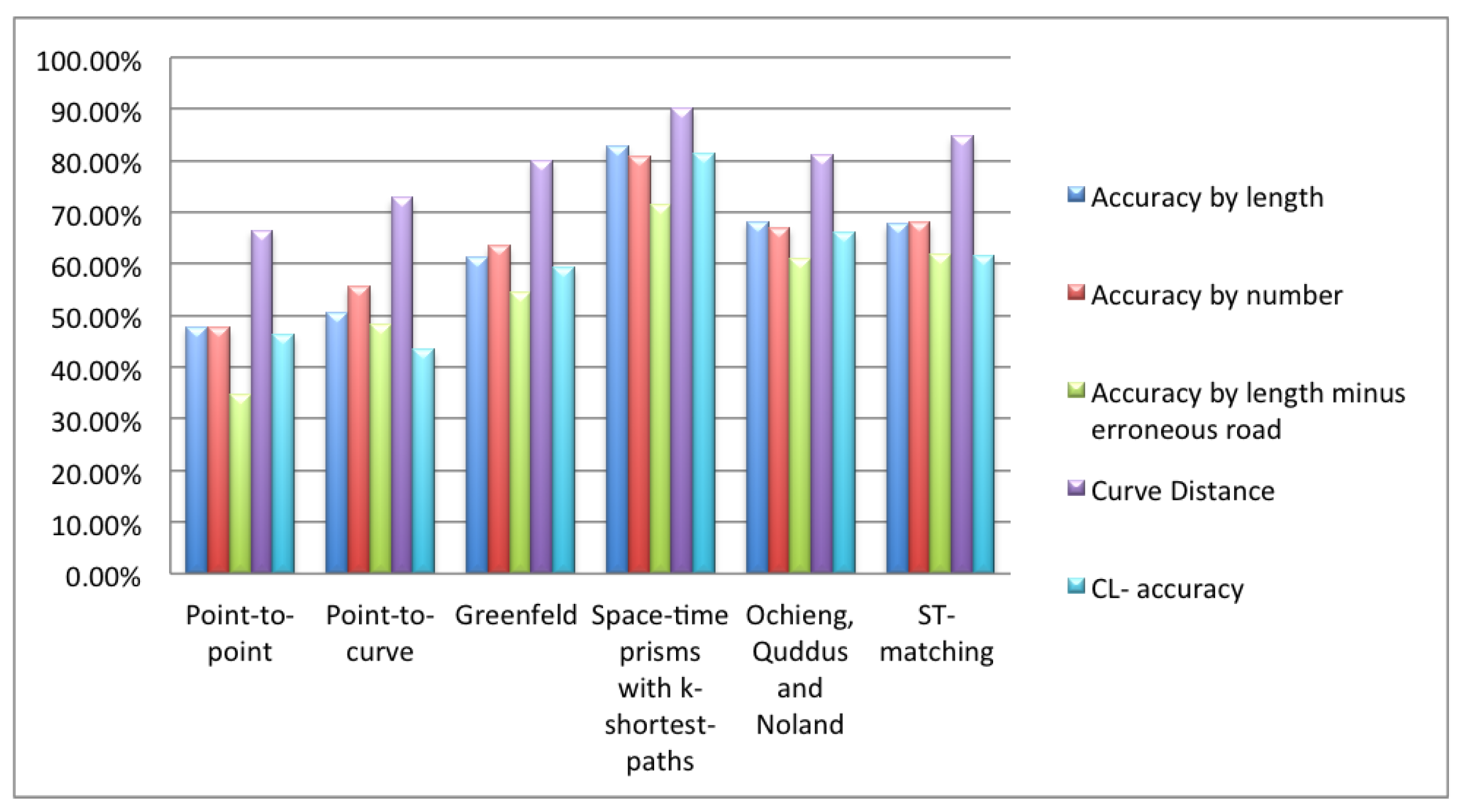
5.3. Discussion
6. Conclusions and Open Problems
Acknowledgments
Author Contributions
Conflicts of Interest
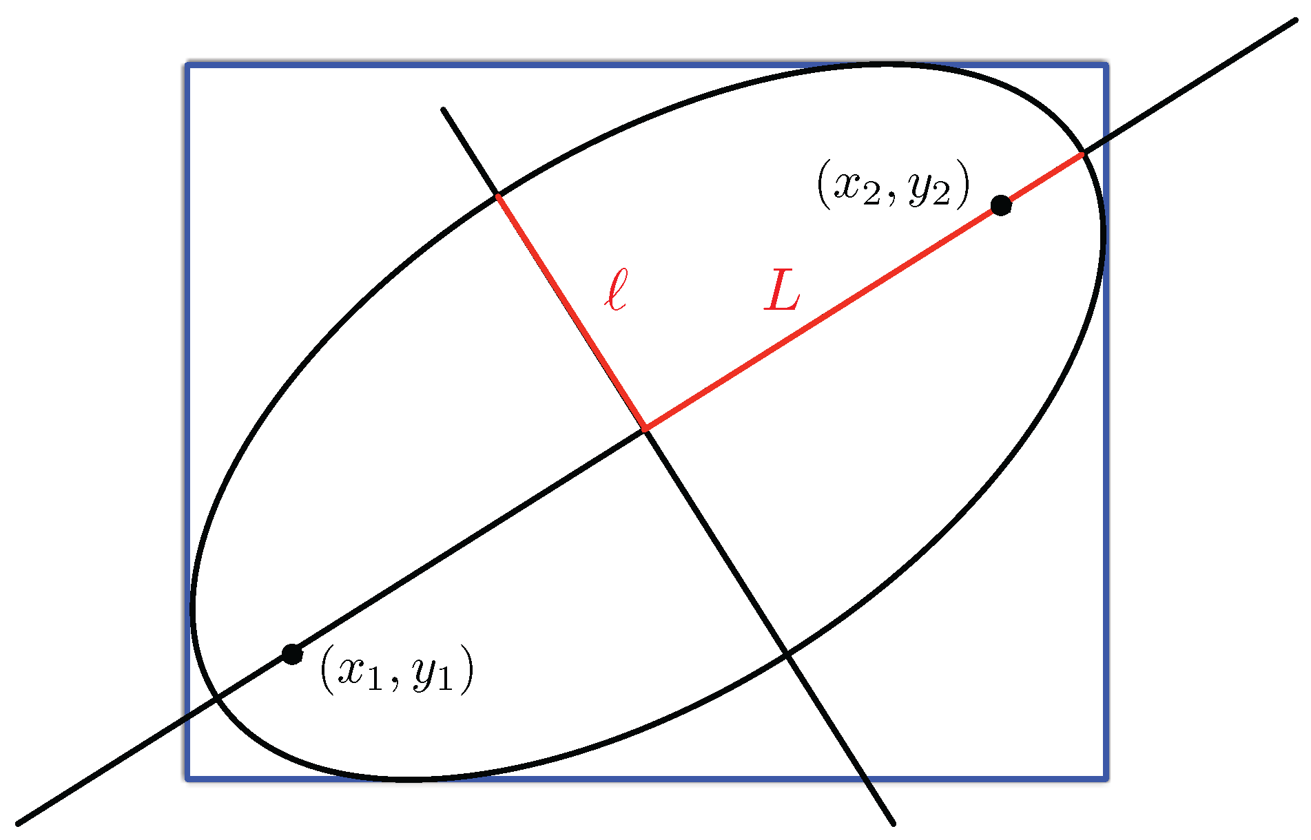
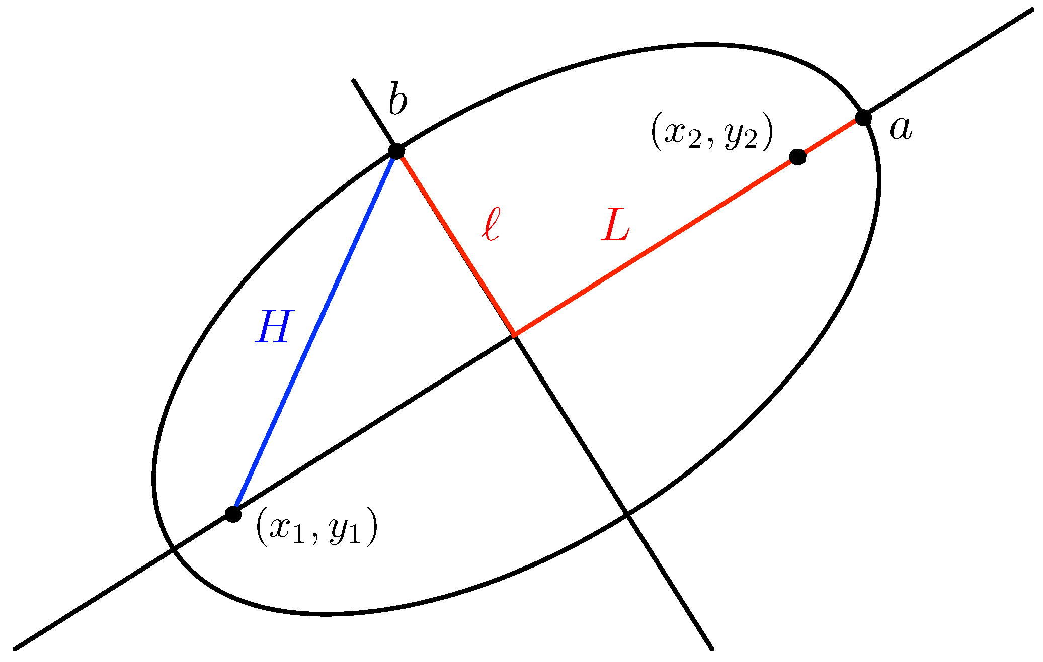
Appendix A. Computation of the Projection of a Space-Time Prism and Its Bounding Box


- If , then:is the equation of the ellipse, and the bounding box is given by , , and ;
- If and , then:is the equation of the ellipse, and the bounding box is given by , , and ;
- If and , then:is the equation of the ellipse, and the bounding box is given by , , and ;
- If and , then:is the equation of the ellipse, and the bounding box is given by:
- and
References
- Giannotti, F.; Pedreschi, D. Mobility, Data Mining and Privacy—Geographic Knowledge Discovery; Springer: Berlin, Germany, 2008. [Google Scholar]
- White, C.E.; Bernstein, D.; Kornhauser, A.L. Some map matching algorithms for personal navigation assistants. Transp. Res. Part C Emerg. Technol. 2000, 8, 91–108. [Google Scholar] [CrossRef]
- Güting, R.H.; Schneider, M. Moving Objects Databases; Morgan Kaufmann: San Francisco, CA, USA, 2005. [Google Scholar]
- Yen, J.Y. Finding the lengths of all shortest paths in N-node nonnegative-distance complete networks using N3 additions and N3 comparisons. J. ACM 1972, 19, 423–424. [Google Scholar] [CrossRef]
- Hashemi, M.; Karimi, H.A. A critical review of real-time map-matching algorithms: Current issues and future directions. Comput. Environ. Urban Syst. 2014, 48, 153–165. [Google Scholar] [CrossRef]
- Bernstein, D.; Kornhauser, A.L. An Introduction to Map Matching for Personal Navigation Assistans; Technical Report; Transportation Research Board: Washington, DC, USA, 1998. [Google Scholar]
- Eddy, S.R. What is a hidden Markov model? Nat. Biotechnol. 2004, 22, 1315–1316. [Google Scholar] [CrossRef] [PubMed]
- Newson, P.; Krumm, J. Hidden Markov map matching through noise and sparseness. In Proceedings of the 17th ACM SIGSPATIAL International Symposium on Advances in Geographic Information Systems, New York, NY, USA, 4–6 November 2009.
- Krumm, J.; Letchner, J.; Horvitz, E. Map matching with travel time constraints. In Proceedings of the Society of Automotive Engineers (SAE) 2007 World Congress, Detroit, MI, USA, 3–6 April 2007.
- Greenfeld, J.S. Matching GPS observations to locations on a digital map. In Proceedings of the Transportation Research Board 81st Annual Meeting, Washington, DC, USA, 13–17 January 2002.
- Brakatsoulas, S.; Pfoser, D.; Salas, R.; Wenk, C. On map-matching vehicle tracking data. In Proceedings of the 31st International Conference on Very Large Data Bases, Toronto, ON, Canada, 31 August–3 September 2005.
- Wenk, C.; Salas, R.; Pfoser, D. Addressing the need for map-matching speed: Localizing global curve-matching algorithms. In Proceedings of the 18th International Conference on Scientific and Statistical Database Management, Vienna, Austria, 3–5 July 2006.
- Kalman, R.E. A new approach to linear filtering and prediction problems. Trans. ASME J. Basic Eng. 1960, 82, 35–45. [Google Scholar] [CrossRef]
- Quddus, M.A.; Zhao, L.; Ochieng, W.Y.; Noland, R.B. An extended Kalman Filter algorithm for integrating GPS and low-cost dead reckoning system data for vehicle performance and emissions monitoring. J. Navig. 2003, 56, 257–275. [Google Scholar]
- Li, L.; Quddus, M.; Zhao, L. High accuracy tightly-coupled integrity monitorin algorithm for map matching. Transp. Res. Part C Emerg. Technol. 2013, 36, 13–26. [Google Scholar] [CrossRef] [Green Version]
- Quddus, M.A.; Ochieng, W.Y.; Noland, R.B. Map matching in complex urban road networks. Braz. Jm Cartogr. Revista Brasil. Cartogr. 2003, 55, 1–18. [Google Scholar]
- Zadeh, L.A. Fuzzy sets. Inf. Control 1965, 8, 338–353. [Google Scholar] [CrossRef]
- Zhao, Y. Vehicle Location and Navigation Systems: Intelligent Transportation Systems; Navtech Seminars and GPS Supply: Alexandria, VA, USA, 1997. [Google Scholar]
- Syed, S.; Cannon, M.E. Fuzzy logic based map matching algorithm for vehicle navigation system in urban canyons. In Proceedings of the 2004 National Technical Meeting of the Institute of Navigation, Monterey, CA, USA, 26–28 January 2004.
- Quddus, M.A. High Integrity Map Matching Algorithms for Advanced Transport Telematics Applications. Ph.D. Thesis, Imperial College, London, UK, 2006. [Google Scholar]
- Lou, Y.; Zhang, C.; Zheng, Y.; Xie, X.; Wang, W.; Huang, Y. Map-matching for low-sampling-rate GPS trajectories. In Proceedings of the 17th ACM SIGSPATIAL International Symposium on Advances in Geographic Information Systems, Seattle, WA, USA, 4–6 November 2009.
- Li, Y.; Huang, Q.; Kerber, M.; Zhang, L.; Guibas, L. Large-scale joint map matching of GPS traces. In Proceedings of the 21st ACM SIGSPATIAL International Conference on Advances in Geographic Information Systems, New York, NY, USA, 5–8 November 2013.
- Tang, J.; Song, Y.; Miller, H.J.; Zhou, X. Estimating the most likely space–time paths, dwell times and path uncertainties from vehicle trajectory data: A time geographic method. Transp. Res. Part C Emerg. Technol. 2016, 66, 176–194. [Google Scholar] [CrossRef]
- Chen, B.Y.; Yuan, H.; Li, Q.; Lam, W.H.K.; Shaw, S.; Yan, K. Map-matching algorithm for large-scale low-frequency floating car data. Int. J. Geogr. Inf. Sci. 2014, 28, 22–38. [Google Scholar] [CrossRef]
- Wang, W.; Jin, J.; Ran, B.; Guo, X. Large-scale freeway network traffic monitoring: A map-matching algorithm based on low-logging frequency GPS probe data. J. Intell. Transp. Syst. 2011, 15, 63–74. [Google Scholar] [CrossRef]
- Miwa, T.; Kiuchi, D.; Yamamoto, T.; Morikawa, T. Development of map matching algorithm for low frequency probe data. Transp. Res. Part C Emerg. Technol. 2016, 22, 132–145. [Google Scholar] [CrossRef]
- Rahmani, M.; Koutsopoulos, H. Path inference from sparse floating car data for urban networks. Transp. Res. Part C Emerg. Technol. 2013, 30, 41–54. [Google Scholar] [CrossRef]
- Hunter, T.; Abbeel, P.; Bayen, A.M. The path inference filter: Model-based low-latency map matching of probe vehicle data. IEEE Trans. Intell. Transp. Syst. 2014, 15, 507–529. [Google Scholar] [CrossRef]
- Zeng, Z.; Zhang, T.; Li, Q.; Wu, Z.; Zou, H.; Gao, C. Curvedness feature constrained map matching for low-frequency probe vehicle data. Int. J. Geogr. Inf. Sci. 2016, 30, 660–690. [Google Scholar] [CrossRef]
- Pfoser, D.; Jensen, C.S. Capturing the uncertainty of moving-object representations. In Lecture Notes in Computer Science; Güting, R.H., Papadias, D., Lochovsky, F.H., Eds.; Springer: Berlin, Germany, 1999; pp. 111–132. [Google Scholar]
- Egenhofer, M.J. Approximation of geospatial lifelines. In SpadaGIS, Workshop on Spatial Data and Geographic Information Systems; Bertino, E., Floriani, L.D., Eds.; University of Genova: Genova, Italy, 2003. [Google Scholar]
- Hornsby, K.; Egenhofer, M.J. Modeling moving objects over multiple granularities. Ann. Math. Artif. Intell. 2002, 36, 177–194. [Google Scholar] [CrossRef]
- Wolfson, O. Moving objects information management: The database challenge. In Lecture Notes in Computer Science; Halevy, A.Y., Gal, A., Eds.; Springer: Berlin, Germany, 2002; pp. 75–89. [Google Scholar]
- Hägerstrand, T. What about people in regional science? Papers Reg. Sci. Assoc. 1970, 24, 7–21. [Google Scholar] [CrossRef]
- Miller, H.J. A measurement theory for time geography. Geogr.l Anal. 2005, 37, 17–45. [Google Scholar] [CrossRef]
- Othman, W. Uncertainty Management in Trajectory Databases. Ph.D. Thesis, Hasselt University, Hasselt, Belgium, 2009. [Google Scholar]
- Hart, P.E.; Nilsson, N.J.; Raphael, B. A formal basis for the heuristic determination of minimum cost paths. IEEE Trans. Syst. Sci. Cybern. 1968, 4, 100–107. [Google Scholar] [CrossRef]
- Dijkstra, E.W. A nnte on two problems in connexion with graphs. Numer. Math. 1959, 1, 269–271. [Google Scholar] [CrossRef]
- Ghys, K.; Kuijpers, B.; Moelans, B.; Othman, W.; Vangoidsenhoven, D.; Vaisman, A.A. Map matching and uncertainty: An algorithm and real-world experiments. In Proceedings of the 17th ACM SIGSPATIAL International Symposium on Advances in Geographic Information Systems, Seattle, DC, USA, 4–6 November 2009.


| Id | Init | A | B | C | D | E | F | G | H | I | J | K | L | M |
|---|---|---|---|---|---|---|---|---|---|---|---|---|---|---|
| 1 | 0 | 3 | 5 | 5 | 5 | 5 | 5 | 5 | 5 | 5 | 5 | 5 | 5 | 5 |
| 2 | 0 | 0 | 0 | 0 | 0 | 0 | 0 | 0 | 0 | 0 | 0 | 0 | 0 | 0 |
| 3 | 0 | 2 | 3 | 3 | 3 | 3 | 3 | 3 | 3 | 3 | 3 | 3 | 3 | 3 |
| 4 | 0 | 1 | 4 | 7 | 7 | 7 | 7 | 7 | 7 | 7 | 7 | 7 | 7 | 7 |
| 5 | 0 | 0 | 0 | 2 | 2 | 2 | 2 | 2 | 2 | 2 | 2 | 2 | 2 | 2 |
| 6 | 0 | 0 | 0 | 0 | 0 | 0 | 0 | 0 | 0 | 0 | 0 | 0 | 0 | 0 |
| 7 | 0 | 0 | 0 | 0 | 0 | 0 | 0 | 0 | 0 | 0 | 0 | 0 | 0 | 0 |
| 8 | 0 | 0 | 0 | 1 | 4 | 5 | 5 | 5 | 5 | 5 | 5 | 5 | 5 | 5 |
| 9 | 0 | 0 | 0 | 0 | 2 | 5 | 7 | 8 | 9 | 9 | 9 | 9 | 9 | 9 |
| 10 | 0 | 0 | 0 | 0 | 1 | 3 | 6 | 9 | 11 | 13 | 13 | 13 | 13 | 13 |
| 11 | 0 | 0 | 0 | 0 | 0 | 0 | 1 | 3 | 6 | 9 | 12 | 12 | 12 | 12 |
| 12 | 0 | 0 | 0 | 0 | 0 | 0 | 0 | 0 | 0 | 1 | 3 | 4 | 5 | 5 |
| 13 | 0 | 0 | 0 | 0 | 0 | 0 | 0 | 0 | 0 | 0 | 0 | 0 | 0 | 0 |
| 14 | 0 | 0 | 0 | 0 | 0 | 0 | 0 | 0 | 0 | 0 | 0 | 0 | 0 | 0 |
| 15 | 0 | 0 | 0 | 0 | 0 | 0 | 0 | 0 | 0 | 0 | 1 | 3 | 5 | 5 |
| 16 | 0 | 0 | 0 | 0 | 0 | 0 | 0 | 0 | 0 | 0 | 0 | 3 | 6 | 9 |
| 17 | 0 | 0 | 0 | 0 | 0 | 0 | 0 | 0 | 0 | 0 | 0 | 0 | 0 | 0 |
| 18 | 0 | 0 | 0 | 0 | 0 | 0 | 0 | 0 | 0 | 0 | 0 | 0 | 0 | 0 |
| Algorithm | Average on |
|---|---|
| 20 Samples | |
| Point-to-point | 77,725 |
| Point-to-curve | 699,015 |
| Greenfeld | 168,845 |
| Space-time prisms | 6015 |
| with k-shortest paths | |
| Ochieng, Quddus and Noland | 721,515 |
| ST-matching | 7,612,535 |
© 2016 by the authors; licensee MDPI, Basel, Switzerland. This article is an open access article distributed under the terms and conditions of the Creative Commons Attribution (CC-BY) license (http://creativecommons.org/licenses/by/4.0/).
Share and Cite
Kuijpers, B.; Moelans, B.; Othman, W.; Vaisman, A. Uncertainty-Based Map Matching: The Space-Time Prism and k-Shortest Path Algorithm. ISPRS Int. J. Geo-Inf. 2016, 5, 204. https://doi.org/10.3390/ijgi5110204
Kuijpers B, Moelans B, Othman W, Vaisman A. Uncertainty-Based Map Matching: The Space-Time Prism and k-Shortest Path Algorithm. ISPRS International Journal of Geo-Information. 2016; 5(11):204. https://doi.org/10.3390/ijgi5110204
Chicago/Turabian StyleKuijpers, Bart, Bart Moelans, Walied Othman, and Alejandro Vaisman. 2016. "Uncertainty-Based Map Matching: The Space-Time Prism and k-Shortest Path Algorithm" ISPRS International Journal of Geo-Information 5, no. 11: 204. https://doi.org/10.3390/ijgi5110204