On the Deterministic Prediction of Water Waves
by
 , and
, and
Marco Klein
1,*, 
Matthias Dudek
2, 
Günther F. Clauss
3,
Sören Ehlers
1,
Jasper Behrendt
4,
Norbert Hoffmann
4 and
Miguel Onorato
5 1
Ship Structural Design and Analysis, Hamburg University of Technology, 21073 Hamburg, Germany
2
Neue Warnow Design & Technology GmbH, 18055 Rostock, Germany
3
Ocean Engineering, Technische Universität Berlin, 10623 Berlin, Germany
4
Mechanical Engineering, Hamburg University of Technology, 21073 Hamburg, Germany
5
Department of Physics, University of Turin, 10125 Torino, Italy
*
Author to whom correspondence should be addressed.
Fluids 2020, 5(1), 9; https://doi.org/10.3390/fluids5010009
Submission received: 19 December 2019
/
Accepted: 27 December 2019
/
Published: 7 January 2020
(This article belongs to the Special Issue Nonlinear Wave Hydrodynamics)
Abstract
:This paper discusses the potential of deterministic wave prediction as one basic module for decision support of offshore operations. Therefore, methods of different complexity—the linear wave solution, the non-linear Schrödinger equation (NLSE) of two different orders and the high-order spectral method (HOSM)—are presented in terms of applicability and limitations of use. For this purpose, irregular sea states with varying parameters are addressed by numerical simulations as well as model tests in the controlled environment of a seakeeping basin. The irregular sea state investigations focuses on JONSWAP spectra with varying wave steepness and enhancement factor. In addition, the influence of the propagation distance as well as the forecast horizon is discussed. For the evaluation of the accuracy of the prediction, the surface similarity parameter is used, allowing an exact, quantitative validation of the results. Based on the results, the pros and cons of the different deterministic wave prediction methods are discussed. In conclusion, this paper shows that the classical NLSE is not applicable for deterministic wave prediction of arbitrary irregular sea states compared to the linear solution. However, the application of the exact linear dispersion operator within the linear dispersive part of the NLSE increased the accuracy of the prediction for small wave steepness significantly. In addition, it is shown that non-linear deterministic wave prediction based on second-order NLSE as well as HOSM leads to a substantial improvement of the prediction quality for moderate and steep irregular wave trains in terms of individual waves and prediction distance, with the HOSM providing a high accuracy over a wider range of applications.
1. Introduction
Ships and offshore structures are exposed to the sea, limiting the scope of application of offshore operations, from efficient and economic offshore operations in moderate sea states to reliability as well as survival in extreme wave conditions. To classify offshore operating conditions, predefined limiting criteria such as absolute or relative motions are typically combined with a limiting characteristic wave height or sea state based on stochastic analysis in the design process, allowing identifying feasible and infeasible sea states, respectively. Typically, these limiting sea states are further reduced in terms of allowable significant wave heights by insurer and surveyor of offshore operations. This approach limits the applicability of offshore operations strictly as most sea states (in particular in the transition area between feasible and infeasible region of a scatter diagram) will feature favourable wave sequences allowing short-term offshore operations which are elapsed unused. Knowing the future in terms of deterministic prediction of the encountering wave field and structure motion a sufficient time span in advance would allow reducing the downtime as the critical part of an offshore operation typically corresponds to a short time interval of the whole operation. In addition, a decision support system (DSS) based on deterministic wave prediction can also detect critical wave groups in pretended feasible sea states increasing the safety of complex operations. The impact of such a DSS on shipping as warning system (e.g., parametric roll, extreme wave events, extreme motions and structure response) should not be left unmentioned even though the focus may lie on offshore operations.
The established research on deterministic wave prediction comprises two indispensable constituents: sea state registration and wave prediction. The deterministic structure motion prediction based on the wave prediction is a further key element for a DSS but will not be discussed in detail within this paper. For the registration of the future encountering wave field, the surface elevation has to be measured at a certain distance from the prediction point (e.g., location of offshore operation). Different measurement methods are available, from point measurements (e.g., wave buoy) in time domain to surface elevation snapshots taken from the ship’s X-band radar in the space domain. As the focus of the paper lies on wave prediction exclusively, the following brief description of the sea state registration methods are only introduced in order to support the approach presented in this paper without any technical details.
Point measurements are disadvantageous compared to a surface elevation snapshot as a single point measurement cannot provide information regarding the directionality of the sea state. This problem may be solved by using a large array of several point measurement devices in order to identify the directionality of the wave components. However, as the availability of point measurement devices in the open ocean are generally limited, this approach would denote to install such an array prior to the offshore operation excluding a plug-and-play application. In addition, this approach is impractical for DSS of ships or offshore structures with forward speed. A further drawback is the principle of measurement as point measurements denote that the wave field is recorded at a fixed location over a specific time. As a consequence, the prediction time (time between the moment at which the prediction is available and the moment at which the predicted waves physically arrive at the prediction location) is reduced by the recording time, independently of the computational time needed for the used wave prediction method [1,2,3,4].
The ship’s X-band radars provide the surface elevation for domains of several square kilometres including information on directionality. Theoretically, the detected wave field can be available after every revolution of the radar antenna (<2 s), even though time is needed for the inversion of the radar clutter (due to the presence of the waves) to the wave field. In contrast to single point measurements, where a sufficient measuring time is needed for an accurate and sufficiently long prediction, this time lag is only limited by the numerical efficiency of the used algorithm. Unfortunately, the principle of measurements of X-band radars also yield a main drawback as the radar cannot detect wave troughs behind (steep) wave crests. Thus, the accuracy is dependent on the wave inversion algorithm. However, the advantages of using a ship’s X-band radar (plug-and-play, very fast wave registration over a large space domain, directionality of the wave field, and large prediction horizon) seems to outweigh the disadvantages as two commercial prediction systems are available from the companies Applied Physical Sciences Corporation (FutureWaves™ [5]) and Next Ocean™ [6]. Even this paper focusses on wave prediction exclusively, the presented research assumes surface elevation snapshots (taken continuously by a ship board radar at great distance ahead the operational area) as input for the deterministic wave prediction.
One principal point of the development process of deterministic wave prediction is the implementation of very fast algorithms to obtain the predicted wave field in a sufficient time span before the physical wave field arrives at the prediction location. Only a few methods are capable due to the contrary specifications of very fast calculation time and high accuracy at once. The fastest method but also simplest one is the linear theory, which has already been applied for wave prediction applications with promising findings [2,7,8,9,10,11,12,13,14,15]. A Shipboard Routing Assistance system (SRA) based on the continuous ship’s X-band radar measurements of the surrounding seaway were presented by Payer and Rathje [7]. The linear evolution of continuously measured surface elevation snapshots using the ship’s X-band radar are also the basis for a decision support system for Computer Aided Ship Handling (CASH) developed by Clauss et al. [8]. It was shown that this tool can predict the encountering wave field as well as the structure response fairly accurate for moderate long crested sea states. Later, Clauss et al. [12] and Kosleck [2] enhanced this tool to predict the short crested encountering wave field and the corresponding 6DOF motion. Tyson and Thornhill [16,17] applied linear wave prediction using WaMoS II™ on full scale tests evaluating the predictive skills of the linear methods. They showed that for short forecast duration and small to moderate wave steepness, the accuracy of the linear approach is sufficient. In addition, Naaijen and Huijsmans [9,11] as well as Naaijen et al. [10,15] applied linear wave evolution equations for real time wave prediction and ship motion estimation in long as well as short crested waves concluding “that a 60 s accurate forecast of wave elevation is very well feasible for all considered wave conditions and motion predictions are even more accurate”. Due to the simpleness and robustness, the linear approach is an integral part of commercially available prediction system (e.g., FutureWaves™ [13,14], Next Ocean™ [6]).
However, the linear approach implies uncertainties due to its strong simplifications of the water wave problem. Non-linear effects become dominant with increasing wave steepness reducing the accuracy of the linear approach significantly. Non-linear methods enable advanced simulations with high accuracy but at the expense of computation time. One of the few non-linear and numerical efficient methods suitable for wave prediction are the so-called envelope equations of the NLSE framework [18,19,20,21]. Both the NLSE and the modified NLSE (MNLSE) were extensively experimentally and numerically investigated in terms of non-linear wave evolution (e.g., [22,23,24,25,26] among others). Even if the NLSE captures relevant non-linear phenomena and provides good accuracy for sufficiently narrow spectra, it was generally shown that the NLSE is less suitable for the prediction of irregular sea states due to the spectral bandwidth constraint. The MNLSE on the other side provides significant better agreement due to the broadening of the bandwidth constraints (e.g., [22,23,24,25,26]).
Ruban [27] showed that the NLSE is suitable for the prediction of extreme waves applying the Gaussian variational ansatz to the NLSE in order to obtain a semi-quantitative prediction of non-linear spatio-temporal focussing. Farazmand and Sapsis [28] presented a reduced-order prediction of rogue waves using MNLSE. Their procedure is based on the identification of elementary wave groups (EWG) assuming that critical EWGs do not interact with other EWGs within the short-term prediction. The measured irregular sea state is decomposed into EWGs and the evolution and amplitude growth of critical EWGs is determined by precomputed EWGs based on MNLSE. Thus, the numerical effort for the prediction of extreme events is reduced to the proper decomposition of the sea state and identification of the underlying, precomputed EWG. Cousins et al. [29] showed a similar approach: a data-driven prediction scheme for the prediction on extreme events. This approach can also divided into two separate components. The first component provides the data base for the prediction of extreme events, is based on the MNLSE and can be applied prior any real world application. The basis are localized wave groups which are numerically evolved for varying amplitudes and periods resulting in specific group amplification factors. The second component is the real-time extreme wave predictor using field measurements. Within the measurements, coherent wave groups are to be identified and the future elevation is estimated from the data base. Again, the numerical effort is reduced to decomposition of the irregular wave sequence, identification of coherent wave groups, and resulting amplification.
The NLSE as well as MNLSE has also been used for deterministic wave prediction (e.g., [26,30]). Simanesew et al. [30] applied both for the deterministic prediction of long- as well as short-crested sea states in time domain. They showed that both the NLS and MLSN provide sufficient accuracies in long-crested sea states for short forecast distances and horizons. For increasing directionality the quality of the forecast decreases significantly. Of particular note in this investigation is that the linear dispersion behaviour is captured exactly by using the dispersion operator introduced by Trulsen et al. ([21]).
An alternative non-linear method for wave prediction is the numerically efficient high-order spectral method (HOSM) [31,32,33]. Wu [1] as well as Blondel et al. [34] applied the HOSM for the deterministic reconstruction and prediction of non-linear wave fields. The basis of their work are wave registrations based on one or several wave probes at specific locations. Thus, sophisticated optimization procedures for the reconstruction of the wave field in space were used at the beginning as snapshots in the space domain are required as initial condition for the HOSM. This time-consuming reconstruction process hindered an effective application of the HOSM for wave prediction. However, taking advantage of the supposed drawback by using surface elevation snapshots continuously taken by a ship’s X-band radar at great distance as input, enables the use of the efficient and accurate HOSM without time-consuming reconstruction of the wave field in space domain. Nevertheless, they generally showed that long-time and large-space simulations of non-linear sea state evolutions can be performed accurately and efficiently with the HOSM. Clauss et al. [35] and Klein et al. [36] presented that the HOSM predicts non-linear wave group propagation very accurately. The applicability of the HOSM for non-linear real-time prediction was shown by Köllisch et al. [4]. Desmar et al. [37] applied the HOSM for the generation of reference wave snapshots in order to evaluate reconstruction methods of different complexity and the consequences on the prediction accuracy. This investigation showed that non-linear methods for wave reconstruction (based on spatio-temporal optical measurements) are improving the accuracy of the reconstructed initial wave field and prediction.
This paper presents a comparative study on the accuracy of intended wave prediction methods of different complexity. The objective is the evaluation of the applicability of the utilised methods for accurate deterministic wave prediction using irregular sea states. The focus lies on the investigation of the influence of the wave steepness, wave propagation distance and shape of the underlying spectrum. To be consistent with a possible real world application (input snapshots from ship’s X-band radar), the numerical and experimental investigations are performed in space domain. Herein, the unavoidable radar shadow around the ship’s position is also modelled and the influence is evaluated. For the experiment’s validation, a semi-experimental validation procedure is introduced as measuring the surface elevation in space domain is almost impractical in the controlled environment of a seakeeping basin. The accuracy of the predictions is evaluated with the surface similarity parameter allowing an exact, quantitative evaluation.
2. Wave Theory
We now present a brief description of the water wave problem without attempting to be comprehensive, herein only those methods are presented which are relevant for this paper. At the beginning the boundary value problem of potential flow theory is briefly introduced, followed by the used methods presented in the order of complexity, from linear wave theory via weakly non-linear envelope equations to (fully) non-linear simulations. At the end, the fully non-linear numerical wave tank waveTUB is additionally presented as waveTUB depict the key element for the semi-experimental validation procedure. For this study, the water wave problem is simplified to long-crested waves.
Assuming that the Newtonian fluid is incompressible, inviscid and irrotational, the evolution of long-crested waves (travelling in x-direction) can be mathematically described by the following governing equations:
with , and the subscripts represent the corresponding derivation. The bottom and the unknown free surface representing the boundaries of the fluid domain. Equation (4) presents the boundary condition at the bottom which is considered to be level, rigid and impermeable. For the dynamic boundary condition at the free surface (Equation (3)), the dynamic pressure is defined to be constant equalling the atmospheric pressure. The kinematic boundary condition at the free surface (Equation (2)) defines that particles, being element of the free surface at rest, must not leave the free surface in the presence of waves. The kinematic as well as dynamic boundary condition have to be fulfilled at the unknown free surface complicating the solution of the boundary value problem significantly.
2.1. Linear Wave Theory
Linear wave theory can be deduced from the Cauchy problem (Equations (1)–(4)) by applying perturbation theory for the unknown potential and surface elevation. In addition, the boundary value problem at the unknown surface can be approximate by Taylor series expansion. For Stokes wave theory, the perturbation parameter is related to the wave steepness . Truncation of the series expansion at order (assuming that the wave height is significantly smaller compared to the wave lengths) results in a simplified boundary value problem for which the analytical linear solution can be determined. For irregular surface elevations of long-crested waves in time and space, the solution reads
with , , and as amplitude, wave number, angular frequency and phase of the component wave. The desired sea state is regarded as superposition of independent harmonic component waves, each with a particular amplitude, frequency and phase. Applying Equation (5), a measured irregular surface elevation can be transformed at any position in time and space enabling a very fast and simple approach for deterministic wave prediction. The analytical basis for irregular sea states is the Fourier transform. The angular frequency and wave number are coupled via the dispersion relation
with water depth d and gravitational acceleration g. The linear description of the natural seaway enables a simple handling of a complex process with widely acceptable results for engineering applications.
2.2. Non-Linear Schrödinger-Type Equations
The classical NLSE can be derived similarly to the linear theory by applying perturbation and Taylor series expansions on the Cauchy problem [18,19]. Assuming small amplitude waves and a narrow bandwidth spectrum, the perturbation parameters are the wave steepness and the relative bandwidth (assuming ). The Taylor series expansions about still water level is introduced in order to simplify the surface boundary conditions. Furthermore, the boundary value problem is separated into the different orders and each order is solved sequentially from the lowest to the highest order. Truncation of the perturbation expansion at order leads to the NLSE. The NLSE captures some important aspects of non-linearity of water waves such as modulation instability and provides exact solutions enabling fundamental research on weakly non-linear wave-wave interaction. However, the NLSE is limited in non-linearity magnitude and spectral bandwidth hindering a diversified application as deterministic wave prediction method. These limitations can be reduced by including higher order terms of the asymptotic series expansion. The next higher order leads to the well known MNLSE [20,21]. Brinch-Nielsen and Johnson [38] derived the MNLS for arbitrary water depth. However, in most of the cases, the MNLSE is applied assuming infinite water depth and is typically referred as Dysthe equation. Recently, Slunyaev and Pelinovsky [39] extended the Dysthe equation to the next order () referring to higher-order Dysthe equation.
Generally, and not only with regard to this study, the water depth influence cannot be neglected for deterministic wave prediction as offshore operations are conducted in arbitrary water depth. For the NLSE, the derivation of the necessary coefficients taking the water depth influence into account can be found in Mei [40]. For the next higher order, Sedletsky [41] derived a second-order NLSE () for arbitrary water depth, which reduces to the classical Dysthe equation in the limit of infinitely deep water. Based on this outcome, Slunyaev [42] derived the third-order NLSE () for arbitrary water depth investigating the impact of the different non-linearity orders on the modulation instability. For this study on deterministic wave prediction, the NLSE up to the second-order is used in the following ways.
According to Slunyaev [42], truncation of the perturbation expansion at order leads to the temporal evolution equation
with A being the envelope of the wave sequence, V the group velocity of the carrier wave, the superscript * denotes conjugate complex. The indices of the coefficients and mark the specific order of the underlying harmonic (first index) as well as order of expansion (second harmonic), which is adopted from Slunyaev [42] in order to be consistent with the presented equations for the coefficients (summarized in Appendix A). The group velocity depends on the carrier wave number , the corresponding angular frequency and the water depth d,
The first four terms in Equation (7) display the classical first order NLSE and the underlying wave field can be reconstructed as follows:
Truncation at order results in Equation (7) representing the solution for the second order NLSE () equivalent to the MNLSE (and Dysthe equation for ). The reconstruction formula reads
with contributions of the zeroth, first and second harmonics.
The dispersive behaviour of the waves is represented by the second term and all terms related to ; the non-linear wave-wave interaction corresponds to the terms. The dispersive terms in Equation (7) are the consequence of the Taylor series expansion of the linear dispersion relation so that the dispersion of the waves is represented in the vicinity of the underlying carrier wave number . For increasing order, the obtained dispersion behaviour approximates to the full linear dispersion. However, Trulsen et al. [21] introduced the full linear dispersion operator
with k representing an array of wave numbers and the higher order dispersive terms can be calculated by
with marks the Fourier transform and the inverse Fourier transform, i.e., the operation is done in Fourier space by means of pseudo-spectral approach. Equation (12) takes terms beyond the highest order () considered in this paper into account and is formally not consistent with the series expansions truncated at specific orders. Nevertheless, introducing Equation (12) into Equation (7) provides the advantage that the linear dispersive behaviour is fully taken into account resulting in increasing accuracy compare to the classical Taylor series expansion of the linear dispersion relation at each selected order. Another advantage is more practical, as in particular for the determination of higher order derivatives via pseudo-spectral methods, the difficulties with numerical noise and aliasing effects are reduced.
For this study, the two non-linear envelope equations resulting from Equation (7) are implemented in order to investigate the influence of the different orders on the wave prediction accuracy. For each order, the full dispersion operator (Equation (12)) is applied. In addition, the Taylor series expansion of the linear dispersion is also applied for the NLSE (first four terms in Equation (7)) to investigate and evaluate the benefit of applying the full dispersion operator. The classical NLSE simulations including Taylor series expansion of the linear dispersion are performed by implementing the pseudo-spectral split-step method. Hereby, the linear and non-linear part of the NLSE are determined separately. The linear part is calculated in frequency domain applying Fourier transform and the non-linear part in time domain. For all other simulations including the full dispersion operator, the linear and non-linear parts are determined together with a pseudo-spectral approach at each time step and advanced in time with the midpoint finite-difference approximation. The carrier ware number necessary to run the simulations is determined for each snapshot by applying
with E the variance spectrum of the snapshot and as weighting factor to weight the result toward the visual peak [43].
2.3. High-Order Spectral Method
The HOS method was introduced independently by West et al. [31] and Dommermuth and Yue [32] (cf. Tanaka [33]). This procedure enables the non-linear simulation of short-crested sea states and takes all non-linear interactions, resonant and non-resonant, into account. In addition, wave-current as well as wave-bottom interactions can be considered. For our investigation, the numerical procedure presented in West et al. [31] is implemented using a pseudo-spectral method. Specifically, all derivatives related to the potential and surface elevation are determined in Fourier space assuming periodic boundary conditions while the non-linear products are calculated in physical space. “The (near) linear computational effort” as well as “exponential convergence (...) are notable characteristics of the computational efficacy of HOS methods” [44].
At the beginning, the Cauchy problem is converted to equations at the free surface . Using chain rules, the free surface boundary conditions (Equations (2) and (3)) can be rewritten as:
with as vertical velocity at the free surface.
Using Equations (14) and (15) as free surface boundary conditions, the boundary value problem is now exclusively related to the vertical velocity (in space domain) and the solution for in terms of and can be determined by series expansion. The procedure proposed by West et al. [31] starts from the formal expression that the velocity potential and vertical velocity can be represented as Taylor series expansion a . Assuming that and are quantities of , and are expanded by perturbation series, with as ordering parameter and is the order of approximation of non-linearity. Separating the terms of each order yields,
for the first order. The next higher order solutions are obtained successively from the next lower order solution,
The vertical velocity W at the surface is obtain by
Assuming periodic boundary conditions, the Fast Fourier Transform (FFT) can be used for determining and its derivatives as well as . For arbitrary water depth, the wave-bottom interaction on can be derived in Fourier space by
with as Fourier coefficient.
For this study, a low pass filter according to West et al. [31] is implemented to avoid Fourier space aliasing for the higher order terms and the series expansion was expanded up to the fourth order (). To suppress high frequency contamination occurring for the highest waves, which can cause numerical instabilities [35], an exponential damping term was additionally introduced in the Fourier space. However, the procedure is neither capable of simulating steep waves close to breaking nor handling wave breaking effects. In this study, the fourth order Runge-Kutta-Gill method is applied to advance the evolution equations in time.
2.4. WaveTUB
This potential theory solver was developed at the Technische Universität Berlin (TUB) for the simulation of non-linear wave propagation [45]. The two-dimensional, non-linear free surface flow problem (Equations (1)–(4)) is solved in time domain. The velocity potential is calculated in the entire fluid domain with the Finite Element Method and at each time step a new boundary-fitted mesh is created. Based on the calculated velocity potential, the velocities at the free surface are determined by second-order differences. The fourth-order Runge-Kutta formula is applied to develop the solution in time domain. At one side of the numerical wave tank, a numerical beach is implemented by adding artificial damping terms to the kinematic and dynamic free surface boundary condition enabling long term simulations. On the other side, a moving wall is implemented for the generation of waves enabling the simulation of piston-type, flap-type and double flap-type wave boards. A detailed description of the theoretical background can be found in Steinhagen [45]. The established program waveTUB showed a high accuracy over recent years for a multitude of different tasks (cf. [45,46,47]).
3. Experimental Program and Results
The following study comprises investigation of irregular sea states based on JONSWAP spectra evaluating the influence of wave steepness, the shape of the underlying spectrum (in terms of enhancement factor ) and the wave propagation over large distances. The above introduced intended wave prediction methods are used and the accuracy is evaluated quantitatively. A realistic real world application is simulated by taking eight consecutive snapshots per sea state (similar to a ship’s radar) into account. In addition, the unavoidable radar shadow is also modelled and its influence on the prediction accuracy is discussed. Following, all data are presented in full scale (model scale 1:75).
Table 1 presents the investigated sea states based on JONSWAP spectra with varying significant wave height and enhancement factor . Therefore, three different significant wave heights are investigated based on preselected wave steepness marking small, moderate and steep irregular sea states. For each wave steepness, the enhancement factor is varied. A special feature of this investigation is the implementation of an identical phase distribution (at the wave board) for all investigated sea states. This allows an exclusive evaluation of the influence of wave steepness and bandwidth of the underlying spectrum. Thus, differences in the evolution of the sea states (and thus to the accuracy of the intended prediction methods) are exclusively related to the underlying wave spectrum allowing conclusions on the effect of non-linear wave propagation due to wave steepness as well as band width of the spectrum.
The experiments are performed in the seakeeping basin of the Ocean Engineering Division at TUB. The basin is 110 m long and 8 m wide with a measuring range of 90 m. The water depth is 1 m. The waves are generated by an fully computer controlled, electrically driven wave generator, which can be used in piston as well as flap-type mode. The implemented wave generation software enables the generation of regular waves, transient wave packages, irregular sea states as well as tailored (critical) wave sequences. On the opposite side, a wave damping slope is installed to suppress disturbing wave reflections.
The accuracy of the different wave prediction methods applied on the measured irregular sea states is investigated with an semi-experimental approach. The aforementioned real world application—deterministic wave prediction based on ship’s X-band radar—serves as prototype. Thus, surface elevation snapshots in space domain are used as input. In addition, fixed prediction locations are defined at which the prediction in time domain is presented. The influence of the radar shadow on the prediction accuracy is additionally investigated. To avoid time-consuming and expensive series of measurements, which would be necessary to detect the surface elevation in space domain in the seakeeping basin, a semi-experimental approach is introduced for the preparation of the input snapshots. Measuring the surface elevation in space domain would denote that plenty of successive, pointwise measurements have to be conducted (with suitable calm down time in between) to obtain the snapshot.
The semi-experimental approach enables significantly fewer measurements by more validation scenarios at the same time. The fully non-linear numerical wave tank waveTUB is applied for the determination of the required surface elevation snapshots for the deterministic wave prediction. The seakeeping basin, used for the experimental validation, can be modelled exactly with this numerical wave tank (including the wave maker) resulting in identical boundary conditions at the wave board, i.e., providing an identical starting point of the wave evolution for both tanks. Thus, the irregular sea states are investigated in the seakeeping basin and reproduced with the numerical wave tank waveTUB providing the input wave snapshots for the deterministic wave prediction. The input snapshots based on waveTUB as well as the prediction results are experimentally validated.
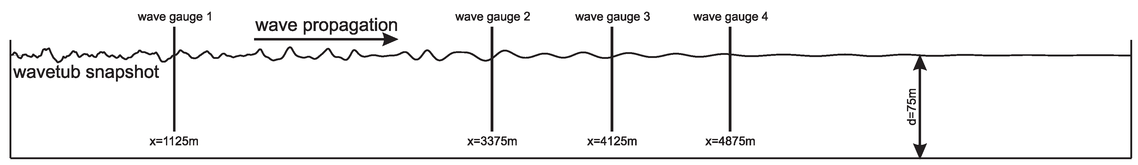
Figure 1 presents the general scheme of this procedure showing the side view on the wave tank (all data full scale). On the left hand side the wave maker and on the right hand side a wave damping beach is installed/modelled. A surface elevation snapshot at a specific time is also indicated which is the basis for the intended wave prediction methods. For the pointwise validation of the waveTUB input snapshots as well as wave predictions by measurements in time domain at fixed positions, four wave gauges are installed during the experiments. The waveTUB reproductions are compared with the experiments near the wave maker at wave gauge 1 to draw conclusions on the quality of the reproduction. The predicted wave sequences for three different prediction distances are validated at the other three wave gauges (2-4).
The waveTUB simulations are used to extract eight consecutive snapshots from each sea state simulating consecutive snapshots taken from the ship’s radar of a real world application. Each consecutive snapshot is used as input for the wave prediction for the three location (cf. Figure 1 wave gauges (2-4)). Figure 2 presents exemplary the applied procedure in detail for sea state 1. The surface elevation snapshots (grey curves) taken from the waveTUB simulations are presented in the left diagrams—the consecutive time steps are displayed from top to bottom. In dependence on the real world application, the real world radar shadow close to an offshore structure is simulated by modifying the waveTUB results. Assuming that wave gauge 2 is the location of the radar and a realistic radar shadow of 500 m, the radar shadow is simulated by changing the surface elevation to zeros in this area (as well as behind wave gauge 2). The modified surface elevation snapshots are shown as red curves in the left diagrams of Figure 2. In addition, the positions of the four wave gauges used in the experiments are indicated by the black vertical lines.
The measured surface elevations (blue curves) in time domain at wave gauge 2 are exemplary compared with the HOSM simulations (red curves) on the right hand side of Figure 2—the prediction basis are the modified waveTUB input snapshots (red curves on the left hand side). Only the time span where an accurate prediction can be accomplished theoretically is presented. This prediction region marks the spatio-temporal domain which can be predicted based on known ranges in space and time for certain sea states. The group velocity of the fastest and slowest wave groups within the sea state define the prediction range—the slowest wave group must have reached the target location (position of offshore structure or in our study the positions of wave gauges 2-4) and the fastest wave group must not have passed the target location (cf. [1,2,3,48]). For this study, the prediction region is determined for each consecutive input snapshot separately but the variation for the different consecutive snapshot as well as sea states is marginal. Based on this, the average prediction time at wave gauge 2 is approximately s (cf. red curves in Figure 2 on the right hand side) with an average minimum forecast horizon time s (time the slowest wave group within the sea state needs to reach the target location, i.e., starting point of the prediction range) and an average maximum forecast horizon s neglecting any computational time (wave gauge 3: s, s and s; wave gauge 4: s, s and s). Please note that these values depend strongly on the dominant wave length and the underlying wave spectrum, i.e., with increasing wave length the forecast horizon will decrease.
The measured and calculated wave sequences at specific locations in time domain are evaluated quantitatively applying the surface similarity parameter (SSP) [49]. The SSP represents “a quantitative method to compare temporal or spatial series in one dimension or temporal or spatial surfaces in two dimensions” [49]. The SSP is a normalized error between two signals or surfaces written in terms of Sobolev norms
with as Fourier transform of the two signals. The magnitude of the SSP varies between 0 (perfect agreement) and 1 (perfect disagreement). One important advantage compared to other available coefficients is the inclusion of both the amplitude and the phase difference of two series or surfaces [49].
Figure 3 and Figure 4 present the accuracy of the predicted wave sequences compared to the measurements for all investigated methods. For the sake of clarity, the results are divided into Figure 3 comparing all NLS-related findings and Figure 4 comparing the accuracy of linear transformation, second-order NLSE and HOSM.
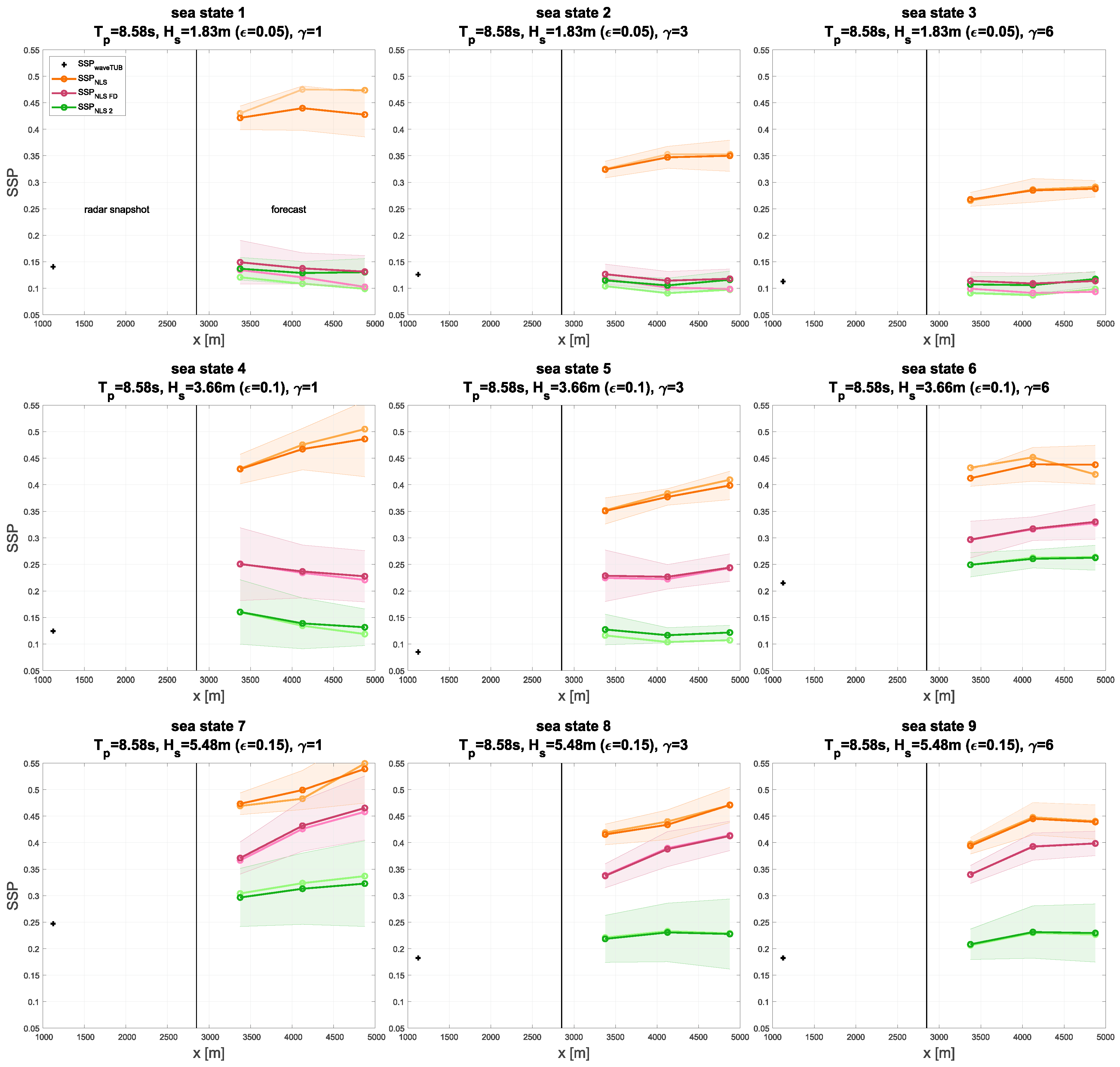
Figure 3 presents the SSP of the waveTUB input snapshot (black plus), the classical first-order NLSE (orange curves), the first-order NLSE including full dispersion operator (NLSEFD, magenta curves) as well as the second-order NLSE (NLSE2, green curves) simulations for the investigated sea states. The darker illustrated curves represent the prediction accuracy including the radar shadow and the lighter illustrated curves display the accuracy without radar shadow. The dots on the curves illustrate the positions of the three wave gauges. The SSP for the predicted sea states represents the mean value of the eight consecutive forecasts. The corresponding variance for the prediction with radar shadow is presented by the transparent areas around the respective curves (with the same colour). The SSP for the waveTUB input snapshot is calculated for the whole time trace at wave gauge 1. Each row presents sea states with constant wave steepness but increasing enhancement factor from left to right and each column sea states with constant enhancement factor but increasing wave steepness from top to bottom. The black vertical line marks the border between “radar” input snapshot (left) and the prediction zone (right).
Noteworthy at a first glance is the influence of the inclusion of the full dispersion operator within the first-order NLSE: the accuracy of the first-order NLSE is significantly improved by taking the full dispersion into account. Based on the underlying simplified assumptions of the NLSE, two main reasons can be identified. On the one hand, the assumed narrow bandwidth of the wave spectrum is not fulfilled for the investigated sea states. Thus, the assumption that the waves within the spectrum evolve with the same group velocity based on a dominant wave length is too inaccurate for deterministic wave prediction of arbitrary irregular sea states. This is clearly supported by the data shown in Figure 3 top as the accuracy of the NLSE increases with increasing enhancement factor (narrower spectrum bandwidth). On the other hand, the range of validity of the NLSE are small amplitude waves. As a consequence, the gain in accuracy with increasing enhancement factor is less distinctive for the steepest irregular sea states. NLSEFD and NLSE2 have the same accuracy for the smallest steepness. This shows, that the NLSE can be applied for broader wave spectra by taking the full dispersion into account. With increasing wave steepness, the advantage of the NLSE2 becomes clear. The accuracy of the NLSEFD decreases with increasing steepness compared to the waveTUB input snapshot accuracy, whereas the accuracy of the NLSE2 is indeed also effected but not so distinct showing a better overall performance also for the steepest cases.
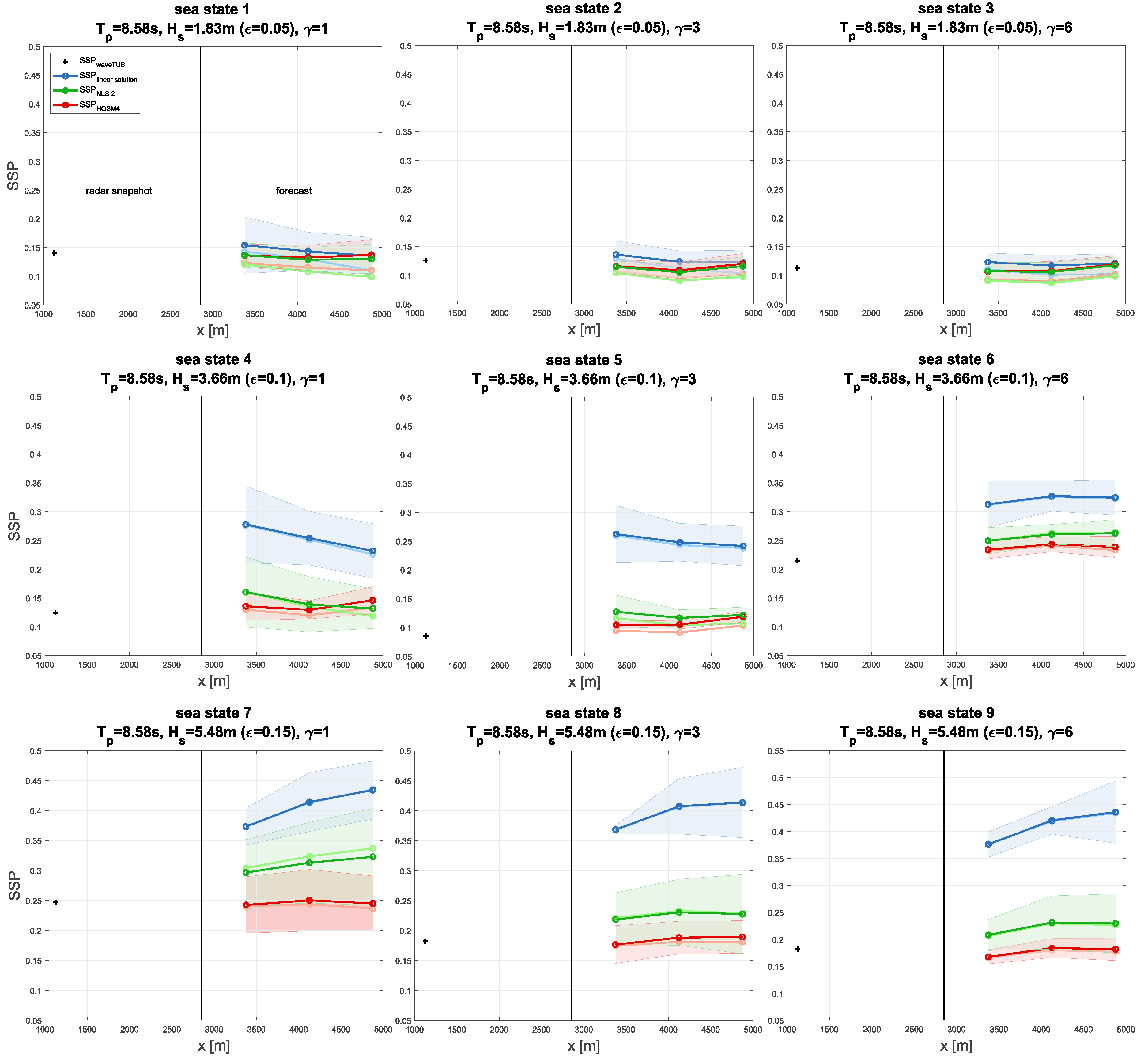
Figure 4 presents the SSP of the waveTUB input snapshot (black plus), the HOSM (red curves), NLSE2 (green curves) as well as linear (blue curves) simulations for the investigated sea states. The diagram is arranged as the previous one, the darker illustrated curves represent the prediction accuracy including the radar shadow and the lighter illustrated curves display the accuracy without radar shadow. The dots on the curves illustrate the positions of the three wave gauges. The SSP for the predicted sea states represents the mean value of the eight consecutive forecasts. The corresponding variance for the prediction with radar shadow is presented by the transparent areas around the respective curves (with the same colour). The SSP for the waveTUB input snapshot is calculated for the whole time trace at wave gauge 1. Each row presents sea states with constant wave steepness but increasing enhancement factor from left to right and each column sea states with constant enhancement factor but increasing wave steepness from top to bottom. The black vertical line marks the border between “radar” input snapshot (left) and the prediction zone (right).
The first row (same small wave steepness and increasing enhancement factor) shows that for small wave steepness the HOSM, the NLSE2 and linear results are in the same accuracy range. This indicates that applying linear transformation for wave prediction of sea states with small wave steepness is sufficient and there is no need for more sophisticated methods. In addition, the three top diagrams reveal that the accuracy of the prediction remains almost constant over a very large distance, i.e., 2025 m or 18 dominant wave length from the beginning of the input snapshot and 4875 m or 43 dominant wave length from the end of the input snapshot to wave gauge 4. The main reason is the fact that for sea states with small wave steepness non-linear effects are very small and these non-linear effects evolve only in a large time and space scale. However, comparing the diagrams of each column shows clearly that with increasing wave steepness (vertical from top to bottom) the accuracy of the linear method decreases whereas the HOSM and NLSE2 are also accurate for steeper sea states. For the steepest investigated sea states, the HOSM prediction is still on the accuracy level of the waveTUB input snapshot over very large distances, whereas the NLSE2 shows to be less accurate. This indicates that the area of application of a forecast tool can be extended significantly by applying more complex wave models. In this context, the HOSM seems to be even applicable for very steep sea states.
Comparing the SSP of NLSEFD (Figure 3) and linear simulation (Figure 4) shows no distinct trend. For the smallest steepness, both methods yield the same accuracy (independently from enhancement factor ). With increasing wave steepness, the accuracy of both methods is still similar with a marginal tendency for better prediction with the NLSEFD.
The influence of the enhancement factor on the prediction accuracy of the HOSM, NLSE2 and linear simulations cannot be determined clearly. No trend is visible for the irregular sea sates with the smallest wave steepness. The discrepancy between linear transformation and HOSM simulation seems to increase slightly for increasing enhancement factor. Hereby, it remains unclear if this is caused by the different accuracies of the input snapshots or due the increase of the enhancement factor. The influence of the radar shadow on the accuracy of the prediction does not show a clear trend. For most of the cases, the influence of the radar shadow is negligible, otherwise the input snapshot without radar shadow provide a slightly improve as well as worsen of the accuracy.
Analysing the accuracy of the waveTUB input snapshot (black plus) reveals that the accuracy of the reproduction decreases with increasing wave steepness. In this context, the diagrams show that the HOSM prediction based on the waveTUB input snapshot remain almost on the same accuracy level (of the waveTUB input snapshot) for all wave steepness. This illustrates clearly that the accuracy of a real world wave prediction tool depends strongly on the accuracy of the detected input wave sequence. Strictly speaking, the wave prediction methods necessary for an accurate prediction are already available and not only the results of this investigation (cf. [10,13,14,15,26,30]) reveals that depending on the specific task very complex and numerically less efficient methods are not necessarily required for a successful application. However, the detection of the surrounding wave field by applying sophisticated wave inversion algorithm on X-band radar clutter is still challenging, but also the crucial factor for a successful application of a wave forecast tool. Hereby, the principle of measurements of X-band radars yield a main drawback as the radar cannot detect wave troughs behind (steep) wave crests. The main challenge hereby is, that most of the relevant applications regarding wave prediction and decision support are related to small wave steepness, where the intensity of the radar clutter is significant smaller compared to more steeper sea states. Less intensity correlates with reduced accuracy, particularly in the far field of the radar reducing the wave prediction horizon. Consequently, the fast linear method accurate enough for small wave steepness is significantly affected by the radar measuring accuracy. In addition, the vessel motions have to be measured accurately (for cruising vessels) in order to determine the position of the X-band radar as a critical prerequisite for the wave inversion. Generally, also the measuring accuracy (radar clutter as well as vessel motion) plays a major role for accurate wave prediction which can be divided in systematic and random error. The mentioned parameters relevant for an accurate wave prediction are only summarized without any detailed discussion as this is out of the scope of this paper.
4. Conclusions
This paper presents a numerical and experimental study on the applicability and limitations of use of intended prediction methods of different complexities: linear wave solution, the NLSE, NLSEFD, NLSE2, and the HOSM. The focus lies on the investigation of the prediction accuracy for varying parameters such as wave steepness, enhancement factor of the JONSWAP spectrum and wave propagation distance. For this purpose, irregular sea states with varying parameters are addressed.
The irregular sea state investigations focusses on JONSWAP spectra with varying wave steepness and enhancement factor. In addition, the influence of the propagation distance as well as the forecast horizon is discussed. The accuracy of the predictions are evaluated quantitatively by the SSP. The results show that the linear method is sufficient for the prediction of irregular sea states with small steepness with the same accuracy as the more complex methods. For increasing wave steepness, non-linear effects are more dominant resulting in a significant decreasing of the accuracy of the linear method. The NLSE results have shown throughout that this method is not applicable for deterministic wave prediction of arbitrary irregular sea states compared to the other methods. However, inclusion of the full dispersion operator resulted in a significant increased accuracy compared to the classical first-order NLSE. Both the NLSE2 and HOSM results illustrate that deterministic wave prediction can be extended to steeper waves by applying more complex wave models. Hereby the HOSM shows a high accuracy also for the steepest investigated sea states over very large distances. In this context, the HOSM prediction based on the waveTUB input snapshot remains almost on the same input snapshot accuracy level for all wave steepness.
The accuracy of the waveTUB reproduction is throughout adequate but showed also that the accuracy decreases with increasing wave steepness of the irregular sea states. This illustrates clearly that the accuracy of a real world wave forecast tool depends strongly on the accuracy of the detected input wave sequence, i.e., assuming a radar-based wave detection, an accurate wave inversion algorithm used to extract the deterministic wave field from the radar clutter is the crucial factor for a successful application of a wave forecast tool.
Author Contributions
Conceptualization: G.F.C., M.K., S.E. and N.H.; methodology: G.F.C., M.K., M.O., S.E. and N.H.; software: M.K., M.O. and J.B.; validation: M.D. and M.K.; formal analysis: M.K. and M.D.; investigation, M.D. and M.K.; writing—original draft preparation: M.K.; writing—review and editing: M.K.; visualization: M.K.; supervision: M.K.; project administration: G.F.C. and M.K.; funding acquisition: G.F.C. and M.K. All authors have read and agreed to the published version of the manuscript.
Funding
This paper is published as a contribution to the joint research project “PrOWOO”. The authors wish to express their gratitude to the German Federal Ministry of Economic Affairs and Energy (BMWi) and Project Management Jülich (PtJ) for funding and supporting the joint research project (FKZ 03SX358A).
Acknowledgments
G.F.C., M.K. and M.D. want to thank the project partner OceanWaveS. M.K. thanks Alexey Slunyaev for fruitful discussions and sharing the subroutine for the calculation of the NLSE coefficients.
Conflicts of Interest
The authors declare no conflict of interest. The funders had no role in the design of the study; in the collection, analyses, or interpretation of data; in the writing of the manuscript, or in the decision to publish the results.
Appendix A
Following the coefficients relevant for implementing Equation (7), which are adopted from Slunyaev [42].
Appendix A.1. Coefficients of Non-linear Interaction Terms
Appendix A.2. Linear Dispersion Coefficients
Appendix A.3. Coefficients of Wave-Induced Flow Components
Appendix A.4. Coefficients in Equations
Appendix A.5. Coefficients Used in Constructing the Wave Field
References
- Wu, G. Direct Simulation and Deterministic Prediction of Large-Scale Nonlinear Ocean Wave-Field. Ph.D. Thesis, Massachusetts Institute of Technology, Cambridge, MA, USA, 2004. [Google Scholar]
- Kosleck, S. Prediction of Wave-Structure Interaction by Advanced Wave Field Forecast. Ph.D. Thesis, Technische Universität Berlin, Berlin, Germany, 2013. [Google Scholar]
- Naaijen, P.; Trulsen, K.; Blondel-Couprie, E. Limits to the extent of the spatio-temporal domain for deterministic wave prediction. Int. Shipbuild. Prog. 2014, 61, 203–223. [Google Scholar] [CrossRef]
- Köllisch, N.; Behrendt, J.; Klein, M.; Hoffmann, N. Nonlinear real time prediction of ocean surface waves. Ocean Eng. 2018, 157, 387–400. [Google Scholar] [CrossRef]
- FutureWaves™. Available online: https://www.aphysci.com/products?id=70 (accessed on 23 January 2019).
- Next Ocean. Available online: http://www.nextocean.nl/ (accessed on 23 January 2019).
- Payer, H.G.; Rathje, H. Shipboard Routing Assistance-Decision Making Support for Operation of Container Ships in Heavy Seas. In Proceedings of the SNAME Annual Meeting, Washington, DC, USA, 29 September–1 October 2004. [Google Scholar]
- Clauss, G.; Kosleck, S.; Testa, D.; Stück, R. Forecast of critical wave groups from surface elevation snapshots. In Proceedings of the OMAE 2007—26th Conference on Offshore Mechanics and Arctic Engineering, San Diego, CA, USA, 10–15 June 2007. [Google Scholar]
- Naaijen, P.; Huijsmans, R. Real time wave forecasting for real time ship motion predictions. In Proceedings of the OMAE 2008—27th Conference on Offshore Mechanics and Arctic Engineering, Estoril, Portugal, 15–20 June 2008. [Google Scholar]
- Naaijen, P.; van Dijk, R.; Huijsmans, R.; El-Mouhandiz, A.A. Real Time Estimation of Ship Motions in Short Crested Seas. In Proceedings of the OMAE 2009—28th Conference on Offshore Mechanics and Arctic Engineering, Honolulu, HI, USA, 31 May–5 June 2009. [Google Scholar]
- Naaijen, P.; Huijsmans, R. Real Time Prediction of Second Order Wave Drift Forces for Wave Force Feed Forward in DP. In Proceedings of the OMAE 2010—29th Conference on Offshore Mechanics and Arctic Engineering, Shanghai, China, 6–11 June 2010. [Google Scholar]
- Clauss, G.F.; Kosleck, S.; Testa, D. Critical Situation of Vessel Operations in Short Crested Seas-Forecast and Decision Support System. ASME J. Offshore Mech. Arct. Eng. 2012, 134, 031601. [Google Scholar] [CrossRef]
- Milewski, P.; Connell, B.; Vinciullo, V.; Kirschner, I. Reduced Order Model for Motion Forecasts of One or More Vessels. In Proceedings of the OMAE 2015—34th Conference on Offshore Mechanics and Arctic Engineering, St. John’s, NL, Canada, 31 May–5 June 2015. [Google Scholar] [CrossRef]
- Kusters, J.G.; Cockrell, K.L.; Connell, B.S.H.; Rudzinsky, J.P.; Vinciullo, V.J. FutureWaves™: A real-time Ship Motion Forecasting system employing advanced wave-sensing radar. In Proceedings of the OCEANS 2016 MTS/IEEE Monterey, Monterey, CA, USA, 19–23 September 2016; pp. 1–9. [Google Scholar] [CrossRef]
- Naaijen, P.; van Oosten, K.; Roozen, K.; van’t Veer, R. Validation of a Deterministic Wave and Ship Motion Prediction System. In Proceedings of the OMAE 2018—International Conference on Offshore Mechanics and Arctic Engineering, Volume 7B: Ocean Engineering, Madrid, Spain, 17–22 June 2018. [Google Scholar] [CrossRef]
- Hilmer, T.; Thornhill, E. Deterministic wave predictions from the WaMoS II. In Proceedings of the OCEANS 2014, Taipei, Taiwan, 7–10 April 2014; pp. 1–8. [Google Scholar] [CrossRef]
- Hilmer, T.; Thornhill, E. Observations of predictive skill for real-time Deterministic Sea Waves from the WaMoS II. In Proceedings of the OCEANS 2015—MTS/IEEE, Washington, DC, USA, 19–22 October 2015; pp. 1–7. [Google Scholar] [CrossRef]
- Zakharov, V.E. Stability of periodic waves of finite amplitude on the surface of a deep fluid. J. Appl. Mech. Tech. Phys. 1968, 9, 190–194. [Google Scholar] [CrossRef]
- Hasimoto, H.; Ono, H. Nonlinear modulation of gravity waves. J. Phys. Soc. Jpn. 1972, 33, 805–811. [Google Scholar] [CrossRef]
- Dysthe, K.B. Note on a modification to the nonlinear Schrödinger equation for application to deep water waves. Proc. R. Soc. Lond. A Math. Phys. Sci. 1736, 369, 105–114. [Google Scholar] [CrossRef]
- Trulsen, K.; Kliakhadler, I.; Dysthe, K.B.; Verlade, M.G. On weakly nonlinear modulation of waves in deep water. Phys. Fluids 2000, 12, 2432–2437. [Google Scholar] [CrossRef]
- Shemer, L.; Kit, E.; Jiao, H.; Eitan, O. Experiments on Nonlinear Wave Groups in Intermediate Water Depth. J. Waterw. Port Coast. Ocean Eng. 1998, 124, 320–327. [Google Scholar] [CrossRef]
- Trulsen, K.; Stansberg, C.T. Evolution of Water Surface Waves: Numerical Simulation and Experiment of Bichromatic Waves. In Proceedings of the Eleventh International Offshore and Polar Engineering Conference, Stavanger, Norway, 17–22 June 2001; International Society of Offshore and Polar Engineers: Mountain View, CA, USA. [Google Scholar]
- Shemer, L.; Kit, E.; Jiao, H. An experimental and numerical study of the spatial evolution of unidirectional nonlinear water-wave groups. Phys. Fluids 2002, 14, 3380–3390. [Google Scholar] [CrossRef] [Green Version]
- Dysthe, K.B.; Trulsen, K.; Krogstad, H.E.; Socquet-Juglard, H. Evolution of a narrow-band spectrum of random surface gravity waves. J. Fluid Mech. 2003, 478, 1–10. [Google Scholar] [CrossRef] [Green Version]
- Hasle, G.; Lie, K.A.; Quak, E. Geometric Modelling, Numerical Simulation, and Optimization; Springer: Berlin/Heidelberg, Germany, 2007. [Google Scholar] [CrossRef]
- Ruban, V.P. Gaussian variational ansatz in the problem of anomalous sea waves: Comparison with direct numerical simulation. J. Exp. Theor. Phys. 2015, 120, 925–932. [Google Scholar] [CrossRef]
- Farazmand, M.; Sapsis, T.P. Reduced-order prediction of rogue waves in two-dimensional deep-water waves. J. Comput. Phys. 2017, 340, 418–434. [Google Scholar] [CrossRef] [Green Version]
- Cousins, W.; Onorato, M.; Chabchoub, A.; Sapsis, T.P. Predicting ocean rogue waves from point measurements: An experimental study for unidirectional waves. Phys. Rev. E 2019, 99, 032201. [Google Scholar] [CrossRef] [PubMed] [Green Version]
- Simanesew, A.; Trulsen, K.; Krogstad, H.E.; Borge, J.C.N. Surface wave predictions in weakly nonlinear directional seas. Appl. Ocean Res. 2017, 65, 79–89. [Google Scholar] [CrossRef] [Green Version]
- West, B.J.; Brueckner, K.A.; Janda, R.S.; Milder, D.M.; Milton, R.L. A new numerical method for surface hydrodynamics. J. Geophys. Res. Ocean. 1987, 92, 11803–11824. [Google Scholar] [CrossRef]
- Dommermuth, D.G.; Yue, D.K.P. A high-order spectral method for the study of nonlinear gravity waves. J. Fluid Mech. 1987, 184, 267–288. [Google Scholar] [CrossRef]
- Tanaka, M. Verification of Hasselmann’s energy transfer among surface gravity waves by direct numerical simulations of primitive equations. J. Fluid Mech. 2001, 444, 199–221. [Google Scholar] [CrossRef]
- Blondel, E.; Ducrozet, G.; Bonnefoy, F.; Ferrant, P. Deterministic Reconstruction and Prediction of a Non-Linear Wave Field using Probe Data. In Proceedings of the OMAE 2008—27th Conference on Offshore Mechanics and Arctic Engineering, Estoril, Portugal, 15–20 June 2008. [Google Scholar]
- Clauss, G.; Klein, M.; Dudek, M.; Onorato, M. Application of Higher Order Spectral Method for Deterministic Wave Forecast. In Proceedings of the OMAE 2014—33rd Conference on Ocean, Offshore and Arctic Engineering, San Francisco, CA, USA, 8–13 June 2014. [Google Scholar]
- Klein, M.; Dudek, M.; Clauss, G.; Hoffmann, N.; Behrendt, J.; Ehlers, S. Systematic Experimental Validation of High-Order Spectral Method for Deterministic Wave Prediction. In Proceedings of the International Conference on Offshore Mechanics and Arctic Engineering, Glasgow, UK, 9–14 June 2019. [Google Scholar]
- Desmars, N.; Pérignon, Y.; Ducrozet, G.; Guérin, C.; Grilli, S.T.; Ferrant, P. Phase-Resolved Reconstruction Algorithm and Deterministic Prediction of Nonlinear Ocean Waves from Spatio-Temporal Optical Measurements. In Proceedings of the OMAE 2018—International Conference on Offshore Mechanics and Arctic Engineering, Madrid, Spain, 17–22 June 2018. [Google Scholar]
- Brinch-Nielsen, U.; Jonsson, I. Fourth order evolution equations and stability analysis for stokes waves on arbitrary water depth. Wave Motion 1986, 8, 455–472. [Google Scholar] [CrossRef]
- Slunyaev, A.; Pelinovsky, E. Numerical Simulations of Modulated Waves in a Higher-Order Dysthe Equation. In Water Waves; Springer: Berlin/Heidelberg, Germany, 2019; pp. 1–19. [Google Scholar]
- Mei, C.C. The Applied Dynamics of Ocean Surface Waves, 2nd ed.; Advanced Series on Ocean Engineering; World Scientific: Singapore, 1989; Volume 1. [Google Scholar]
- Sedletsky, Y.V. The fourth-order nonlinear Schrödinger equation for the envelope of Stokes waves on the surface of a finite-depth fluid. J. Exp. Theor. Phys. 2003, 97, 180–193. [Google Scholar] [CrossRef]
- Slunyaev, A.V. A high-order nonlinear envelope equation for gravity waves in finite-depth water. J. Exp. Theor. Phys. 2005, 101, 926–941. [Google Scholar] [CrossRef]
- Sobey, R.J.; Young, I.R. Hurricane Wind Waves—A Discrete Spectral Model. J. Waterw. Port. Coast. Ocean Eng. 1986, 112, 370–389. [Google Scholar] [CrossRef]
- Mei, C.C.; Stiassnie, M.; Yue, D.K.P. Theory and Applications of Ocean Surface Waves: Nonlinear Aspects; Advanced Series on Ocean Engineering; World Scientific: Singapore, 2005. [Google Scholar]
- Steinhagen, U. Synthesizing Nonlinear Transient Gravity Waves in Random Seas. Ph.D. Thesis, Technische Universität Berlin, Berlin, Germany, 2001. [Google Scholar]
- Clauss, G.F.; Schmittner, C.E.; Stück, R. Numerical Wave Tank—Simulation of Extreme Waves for the Investigation of Structural Responses. In Proceedings of the OMAE 2005—24th International Conference on Offshore Mechanics and Arctic Engineering, Halkidiki, Greece, 12–17 June 2005. [Google Scholar]
- Clauss, G.F.; Klein, M.; Onorato, M. Formation of Extraordinarily High Waves in Space and Time. In Proceedings of the OMAE 2011—30th International Conference on Ocean, Offshore and Arctic Engineering, Rotterdam, The Netherlands, 19–24 June 2011. [Google Scholar]
- Blondel-Couprie, E. Deterministic Reconstruction and Prediciton of Non-Linear Wave-Fields Using Probe Data. Ph.D. Thesis, Ecole Centrale de Nantes (ECN), Nantes, France, 2009. [Google Scholar]
- Perlin, M.; Bustamante, M. A robust quantitative comparison criterion of two signals based on the Sobolev norm of their difference. J. Eng. Math. 2016, 101. [Google Scholar] [CrossRef] [Green Version]
Figure 1.
General scheme of the applied semi-experimental procedure for the irregular sea states investigations including validation locations.
Figure 1.
General scheme of the applied semi-experimental procedure for the irregular sea states investigations including validation locations.

Figure 2.
Detailed overview of the applied wave prediction procedure exemplary for sea state 1.

Figure 3.
Surface Similarity Parameter for the investigated sea states at the three wave gauges for classical NLSE (orange curves), NLSE with full dispersion (magenta curves) as well as second-order NLSE (green curves) simulations in space domain. The darker illustrated curves represent the prediction accuracy including the radar shadow and the lighter illustrated curves display the accuracy without radar shadow. The dots on the curves illustrate the positions of the three wave gauges. The SSP of the waveTUB input snapshots is illustrated as black plus.

Figure 4.
Surface Similarity Parameter for the investigated sea states at the three wave gauges for HOSM (red curves), second-order NLSE (green curves) as well as linear (blue curves) simulations in space domain. The darker illustrated curves represent the prediction accuracy including the radar shadow and the lighter illustrated curves display the accuracy without radar shadow. The dots on the curves illustrate the positions of the three wave gauges. The SSP of the waveTUB input snapshots is illustrated as black plus.


Table 1.
Overview of the investigated irregular sea states.
| No. | |||||
|---|---|---|---|---|---|
| 1 | s | m | 1 | ||
| 2 | 3 | ||||
| 3 | 6 | ||||
| 4 | m | 1 | |||
| 5 | 3 | ||||
| 6 | 6 | ||||
| 7 | m | 1 | |||
| 8 | 3 | ||||
| 9 | 6 |
© 2020 by the authors. Licensee MDPI, Basel, Switzerland. This article is an open access article distributed under the terms and conditions of the Creative Commons Attribution (CC BY) license (http://creativecommons.org/licenses/by/4.0/).
Share and Cite
MDPI and ACS Style
Klein, M.; Dudek, M.; Clauss, G.F.; Ehlers, S.; Behrendt, J.; Hoffmann, N.; Onorato, M. On the Deterministic Prediction of Water Waves. Fluids 2020, 5, 9. https://doi.org/10.3390/fluids5010009
AMA Style
Klein M, Dudek M, Clauss GF, Ehlers S, Behrendt J, Hoffmann N, Onorato M. On the Deterministic Prediction of Water Waves. Fluids. 2020; 5(1):9. https://doi.org/10.3390/fluids5010009
Chicago/Turabian StyleKlein, Marco, Matthias Dudek, Günther F. Clauss, Sören Ehlers, Jasper Behrendt, Norbert Hoffmann, and Miguel Onorato. 2020. "On the Deterministic Prediction of Water Waves" Fluids 5, no. 1: 9. https://doi.org/10.3390/fluids5010009